CFD Modeling of Flame Jump across Air Gap between Evasé and Capture Duct for Ventilation Air Methane Abatement

Abstract

The ventilation air–methane (VAM) released from underground mines is often transported into regenerative thermal oxidizer (RTO) devices and burnt into heat energy. This study numerically investigates the scenarios where explosion occurs inside the RTO and the flame and pressure waves propagate back quickly towards the VAM discharge duct. Possibilities of secondary explosion in the discharge duct, hence in the downstream underground mines, are examined. The results critically showed that when the methane concentration accumulated in the RTO reached 7.5% or above, the flame generated from the explosion jumped to the evasé of the discharge section (over a distance of 29.4 m) and could induce explosions in underground mines.

1. Introduction

In ventilation air–methane (VAM) abatement systems, methane is released from underground mines and subsequently transported into regenerative thermal oxidizer (RTO) devices where exothermic reactions take place [1]. The heat energy liberated from reactions is stored in the ceramic material of RTO. In scenarios where an explosion of air–methane occurs inside the RTO, the flame and pressure waves propagate quickly towards the evasé, a discharge section of a gradually enlarging area. Secondary explosion might occur after the flame propagates to the exit of the evasé and meets the mixture of air–methane that is being vented from underground mines. If the flame propagates further, downstream explosions inside the underground mines might be induced.

To steer clear of the occurrence of these unexpected explosions, no physical connection between mine evasé and the VAM capture duct has been of great interest to the VAM abatement industry. From a technical point of view, direct coupling seems more practical and provides better control of the entire VAM abatement system. However, it also provides an easy path for the flame and pressure waves to propagate from the RTO to the mine evasé, and vice versa. In the no physical connection approach, the ample air gap between the evasé and the capture duct could stop the flame from traveling due to heat loss to the atmosphere. Therefore, it is vital to understand the behavior of the flame jump from the capture duct to the evasé to prevent and mitigate the occurrence of this category of accidental explosions in underground mines. However, relevant studies are scarce in the public domain, which leads to poor understanding of the scenarios where the flame and pressure waves propagate back towards the evasé.

Computer modeling has proved to be a powerful and promising alternative to physical measurements [2,3,4,5,6], particularly when harsh site conditions are present and the resulting capital costs and hazardous risks escalate. A variety of combustion models are available for modeling the explosion of methane–air mixtures, such as the finite-rate kinetics model without a turbulence–chemistry interaction (TCI), the eddy dissipation model (EDM), and the eddy dissipation concept (EDC) model. Generally, the accuracy of the specified or calculated flame speed plays a pivotal role in determining the prediction accuracy of flame propagation. Specification of the flame speed is involved in some approaches (e.g., progress variable (c) based modeling [7,8]), which have to employ empirical factors in the source term, limiting their applicability and prediction accuracy. To tackle this challenge, Van Oijen and colleagues [9,10,11] proposed the flamelet generated manifold (FGM) model and used the model to simulate the deflagration of methane–air mixtures. The authors [9,10,11] tabulated the source terms for the unnormalized reaction progress variable using the detailed chemistry; in so doing, there is no need to specify the flame speed or calibrate the empirical constants.

In this study, we developed a partially premixed combustion model based on the FGM model to numerically investigate the propagation of methane–air combustion flame. The unsteady RANS (URANS) approach was deployed to simulate the transient pressure field along with flame propagation. Extreme cases with high methane concentrations (5–9.5%) accumulated in the RTO have been examined. The main objective is to understand the possibilities for the flame and pressure waves to propagate from the capture duct to the exit of the evasé and subsequently induce secondary explosions in underground mines.

2. Theory and Mathematical Models

2.1. Governing Equations

In the FGM model, a look-up table of the probability distribution function (PDF) for the progress variable (c) and the mixture fraction (f) is generated [9,10,11]. The reaction progress variable (c) is the normalized sum of the mass fractions of the product species, calculated as,

$$c=\frac{{\displaystyle \sum _k}{a}_k(Y_k-Y_k^u)}{{\displaystyle \sum _k}{a}_k(Y_k^{eq}-Y_k^u)}=\frac{Y_c}{Y_c^{eq}},$$

(1)

where $Y_k$ denotes the $k$th species mass fraction. Superscript u is the unburnt reactant at the flame inlet and superscript $eq$ means the chemical equilibrium at the flame outlet and $a_k$ are constants (typically zero for reactants and unity for a few product species). The 1D adiabatic premixed flame equations are transformed from physical-space to reaction-progress space by Equations (2) and (3) for species mass fraction and temperature, respectively,

$$\rho \frac{\partial Y_k}{\partial t}+\frac{\partial Y_k}{\partial c}\dot{w_c}=\rho {\chi }_c\frac{{\partial }^2{Y}_k}{\partial c^2}+\dot{w_k},$$

(2)

$$\rho \frac{\partial T}{\partial t}+\frac{\partial T}{\partial c}\dot{w_c}=\rho {\chi }_c\frac{{\partial }^{2}T}{\partial c^2}-\frac{1}{c_p}\sum _k{h}_k\dot{w_k}+\frac{\rho {\chi }_c}{c_p}(\frac{\partial c_p}{\partial c}+\sum _k{c}_{p,k}\frac{\partial Y_k}{\partial c})\frac{\partial T}{\partial c},$$

(3)

where $h_k$ is the total enthalpy, $c_{p,k}$ is the $k^{th}$ species specific heat at constant pressure, and $\dot{w_k}$ is the $k^{th}$ species mass reaction rate. Differential-diffusion is not considered in these equations. The scalar dissipation rate (${\chi }_c$) is calculated by,

$${\chi }_c=\frac{\lambda }{\rho c_p}{|\nabla c|}^2,$$

(4)

Evidently, the scalar dissipation is an input to the set of equations and varies with c, modeled as,

$${\chi }_c\left(c\right)={\chi }_{max}exp[-2{\left(erf{c}^{-1}\left(2c\right)\right)}^2],$$

(5)

where $erf{c}^{-1}$ is the inverse complementary error function and ${\chi }_{max}$ is a user-specified maximum scalar dissipation within the premixed flamelet. The 1D premixed flamelet is calculated at a single equivalence ratio that can be directly related to a corresponding mixture fraction. Premixed laminar flamelets are generated over a range of mixture fractions for partially-premixed combustion. For different mixture fractions, premixed flamelets have different maximum scalar dissipations, ${\chi }_{max}$. For a given mixture fraction, the scalar dissipation (${\chi }_c(f,c)$) is calculated by,

$${\chi }_c(f,c)={\chi }_{max}^{sto}exp[-2{(erf{c}^{-1}(\frac{f}{f_{sto}}))}^2]exp[-2{(erf{c}^{-1}(2c))}^2],$$

(6)

Subscript $sto$ denotes the stoichiometric mixture fraction, at which the only input required to the premixed flamelet generator is the scalar dissipation, ${\chi }_{max}^{sto}$. A value of 1000 s${}^{-1}$ is used and matches the solutions of unstrained physical space flamelets for rich, lean, and stoichiometric hydrocarbon and hydrogen flames at standard pressure and temperature conditions.

The transport equation for the Reynolds averaged unnormalized progress variable, ${\tilde{Y}}_c$, is expressed as,

$$\frac{\partial (\overline{\rho }{\tilde{Y}}_c)}{\partial t}+\frac{\partial }{\partial x_i}(\overline{\rho }{\tilde{u}}_i{\tilde{Y}}_c)=\frac{\partial }{\partial x_i}(\overline{\rho }{D}_{eff}\frac{\partial {\tilde{Y}}_c}{\partial x_i})+{\overline{S}}_c,$$

(7)

where ${\overline{S}}_c$ is the mean source term, modeled from the finite-rate generated from the premixed flamelet by,

$${\overline{S}}_c=\overline{\rho }\int \int S_{FR}(c,f)P(c,f)dcdf={\overline{S}}_{FR},$$

(8)

${\overline{S}}_c$ determines the turbulent flame position. The finite rate source term, tabulated from the detailed chemistry, is used (i.e., Equation (8), not involving any empirical constants. It is worth emphasizing that this model does not contain any adjustable parameters, which otherwise would be the case for existing models where a correlation is often employed for calculating the turbulent flame speed. As such, no changes to the model are required when applying the model to different methane concentrations or computational domains.

2.2. Computational Domain and Meshing

Figure 1 shows the computational domain and meshing. The capture duct has a length of 30 m and is divided into six subsections. The ignition point is set at the position 0.95 m far away the start of section 1. In the simulation, the dome section and sections 1–3 are set as the explosive zone with the stoichiometric methane concentration ($9.5\%$ mole fraction). Sections 4–6 and the lower ambient space connecting the capture duct and the evasé are filled with different methane concentrations. A uniform mesh size of 3 cm is used for the far end (RTO part), including the dome section, capture duct, front end of capture duct, ambient space (air gap), and the evasé. A gradually coarsening mesh size is used along the height of the top part of the ambient space to save computational time. A total element count of 207,451 is generated for the computational modeling. Detailed numerical methodologies and strategies, and boundary and initial conditions are given the following sections.

2.3. Computational Domain and Meshing

The following assumptions are made in the simulations of methane–air combustion:

• In table construction, mixture fraction and progress variable space, a 64 × 64 grid point resolution is used;
• Flamelets are generated under the pressure of 1 atm; the effect of the pressure change on different quantities is considered;
• The source term of progress variable equation is calculated through the finite rate option (Equation (8));
• The progress variable variance is obtained by solving its transport equation; and
• GRI-Mech 3.0 is used for flamelet generation.

A 2D, transient, axisymmetric model for capturing major properties of 3D flows [12] has been developed using ANSYS Fluent 2020 R2. The gas is treated as incompressible as the airflow examined in this study generally stays subsonic. The unsteady RANS (URANS) approach, specifically the standard $k-ϵ$ turbulence model with standard log-law wall functions, is deployed to model the transient pressure field variation along with flame propagation. URANS represents the computationally cheapest model, but provides reasonable accuracy.

The convective Courant number is kept below 0.1 with a time step of $10\mathsf{\mu }$s, capable of fully resolving the rapid explosion dynamics. The SIMPLE algorithm is applied to enforce pressure-velocity coupling. The least squared cell based method are used to calculate gradients; the bounded second order upwind is used to discretize all convective terms; the bounded second order implicit scheme is used for the transient terms.

In the operation of real systems, methane is released from the evasé and diffuses into the atmosphere; a small portion of methane flows into the capture duct and, hence, the downstream RTO. For this reason and also ensuring fast convergence, the methane diffusion process from the evasé to the atmosphere is simulated prior to igniting the methane–air explosion. The obtained flow field (in particular, turbulence quantities (i.e., k and $ϵ$)) and temperature spatial distribution are used as the initial conditions for the subsequent simulation of methane–air combustion and flame propagation. However, to consider the accidental explosion in the RTO, extreme conditions of methane concentrations throughout the computational domain are manually set to the prescribed values (as described above). To allow for an acceptable turnaround time for solutions, 128 cores distributed on 8 computer nodes (i.e., 16 cores on each node) are utilized for the simulations.

2.4. Boundary Conditions

All walls are treated as no slip and adiabatic given the extremely short time available for heat loss to the wall. The ambient environment (the enclosed air gap) is simulated using the pressure outlet boundary condition with the absolute pressure set to be atmospheric pressure. A non-reflecting boundary condition is used to the pressure outlet to eliminate any effect caused by the limited size of the simulated ambient environment. The non-reflecting condition is also used to the flow inlet of the evasé to consider the large space behind the evasé in real operations. Around the ignition point the progress variable in two computational cells is set to 1 to initiate the combustion.

2.5. Model Validation

This work is part of our research on VAM abatement. The numerical model developed for the research, namely the FGM-based model, applies to problems pertinent to the research of VAM abatement (with different initial/operating and boundary conditions). Several relevant works conducted in our group have been published where extensive validation of the FGM-based combustion model described above has been conducted in our research group using our own experimental data from different perspectives, including evolution of local absolute pressure, local maximum pressure, pressure wave propagation speed, and flame front propagation speed [13,14,15,16]. In these works, the FGM-based model has been applied to solve problems encountered in the operation of real VAM abatement systems, such as the explosion propagation dynamics in large-scale detonation tubes [13,14] and through fixed beds of RTO devices [15]. As the same model is deployed, for conciseness, the model validation is not reiterated in the present study.

3. Results and Discussion

Figure 2 shows the evolution of pressure and temperature fields around the ignition point immediately after ignition is initiated for the case with 7.5% methane in the RTO. For easy identification, the upper half of the tube shows the contour of temperature and the corresponding contour of pressure is shown in the lower half of the tube. Clearly, once ignited ($t=20$ ms), the flame that is spherical laminar initiates propagation of pressure waves. In the preheat zone of the flame front, the temperature of combustion products rises up to 2070 K and heats the surrounding unburnt gases to ignite the subsequent reaction. The expansion of hot gases immediately induces the compression of unburnt gases resulting in a pressure rise of about $50Pa$, matching the theoretical estimation by $\Delta p={\rho }_u{U}_u^2(\frac{{\rho }_u}{{\rho }_b}-1)$ [17]. Local sudden changes in temperature and gas properties lead to subsequent alternate rarefaction and compression of unburnt gases, generating pressure waves. The energy liberated from methane combustion is transmitted mainly through the pressure waves. Moreover, reflections of waves from the surrounding walls, as seen from the increased magnitude of pressure waves, evidently intensifies the wave propagation speed. The local pressure magnitude keeps increasing as more energy is released from methane–air combustion. The strong pressure wave propagation can be readily identified, even at $t=50$ ms with a small region of methane consumed.

The quantitative distribution of temperature, gas density, pressure, and axial velocity along the center line is illustrated in Figure 3 for the case with 7.5% methane in the RTO at $t=50$ ms. The hot gases temperature rises up to 2275 K and correspondingly due to thermal expansion, the hot gases density reduces abruptly. The generated pressure wave propagates towards the exit of evasé. The pressure wave magnitude damps inside the capture duct due to the energy loss through expansion and compression effects of gases along with the propagation of pressure waves. However, there are bounce backs of the pressure magnitudes at locations in between the capture duct inlet and the evasé exit due to reflections from the evasé. Moreover, reflections from the evasé walls lead to strong fluctuation of pressure inside the evasé, as indicated in Figure 3. Likewise, in response to the cycles of rarefaction and compression of unburnt gases, the gas axial velocity also fluctuates with a damping magnitude inside the capture duct. After the inlet of the capture duct, a significant drop in axial velocity is observed due to the expansion of the flow (i.e., flowing into atmosphere). Moreover, corresponding to the reflections of pressure, disturbances in the velocity profile at locations in between the capture duct inlet and the evasé exit and also inside the evasé are observed.

The growth and propagation of flame after ignition inside the capture duct is shown in Figure 4. At $t=10$ ms, the laminar flame propagates uniformly outwards. The elliptical flame shape is formed due to the restrictions of tube walls. Subsequently, the statistically spherical flame transits into a statistically planar geometry after the flame front reaches the tube walls, and propagates towards the tube opening end. However, due to intrinsic instabilities (Darrieus–Landau instability and Rayleigh–Taylor instability) [18,19] the flame front rapidly evolves into a bullet shape ($t=150$ ms). This profile transition has been considered as the main mechanism driving the flame’s acceleration [20]. Furthermore, the flame front is thermodynamically coupled with the pressure wave front (i.e., the combustion heat energy is immediately transmitted to support the pressure wave propagation), leading to the sharp increase in the local maximum pressure. As a result, the flame propagation speed keeps increasing and propagates out of the capture duct as a jet towards the evasé.

Figure 5 shows the time series of temperature contour for the case with 5% methane in the RTO. The evolution of temperature profile is indicative of the process of flame jump from the capture duct to the evasé for this case. After the flame propagates out of the capture duct into the atmosphere, the flame expands and forms a shape of a mushroom that continues to propagate towards the evasé exit. The flame front reaches the evasé exit before $t=0.4$ s. Meanwhile, due to the consumed methane and the heat loss to the atmosphere, the flame extinguishes at the tail of the mushroom and the temperature at the mushroom front drops. After $t=0.5$ s, due to the low methane concentration vented from the evasé, the temperature keeps dropping and at $t=0.7$ s, the flame extinguishes as indicated by the maximum temperature in the vicinity of the evasé that is less than 814 K, i.e., the auto-ignition temperature of methane [16]. Eventually, at $t=1$ s, the temperature in the region surrounding the evasé drops back to the ambient temperature. The results suggest that with 5% methane in the RTO and a distance of 29.4 m between the capture duct and the evasé, the flame cannot jump the gap to induce the secondary explosion in the evasé.

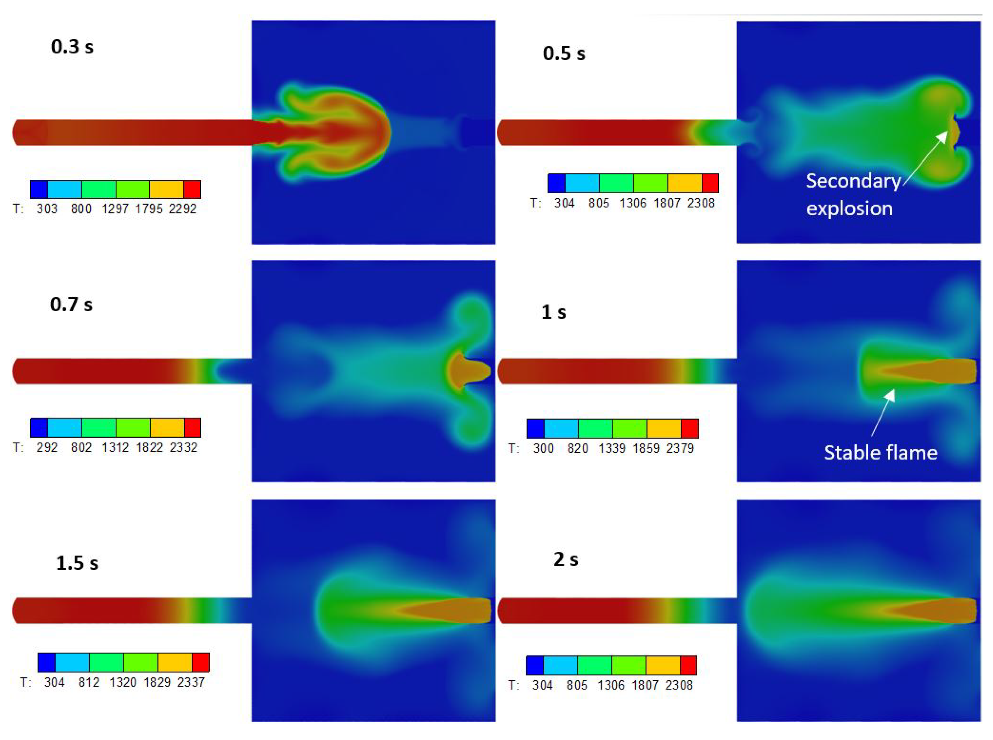
Time series of temperature contour for the case with 7.5% methane in the RTO is shown in Figure 6. Similar to the case with 5% methane concentration, the flame propagates into the atmosphere with the mushroom shape before $t=0.3$ s and due to heat loss, the flame extinguishes at the tail of the mushroom before $t=0.5$ s. However, the temperature inside the evasé is higher compared to that in the case with 5% methane concentration. Subsequently, from $t=0.7$ s, the region of high temperature (>2000 K) inside the evasé keeps expanding outwards, indicating that the secondary explosion occurs. At $t=1$ s, a stable flame shape is formed releasing energy from the combustion to the surrounding. Correspondingly, the region of high temperature expands whilst the length of the flame does not change much. At $t=2$ s, the hot region expands to the mouth of the capture duct. This result critically implies that with the distance of $29.4$ m, the flame can reach the evasé and incur the secondary explosion if the methane concentration reaches $7.5\%$ or above).

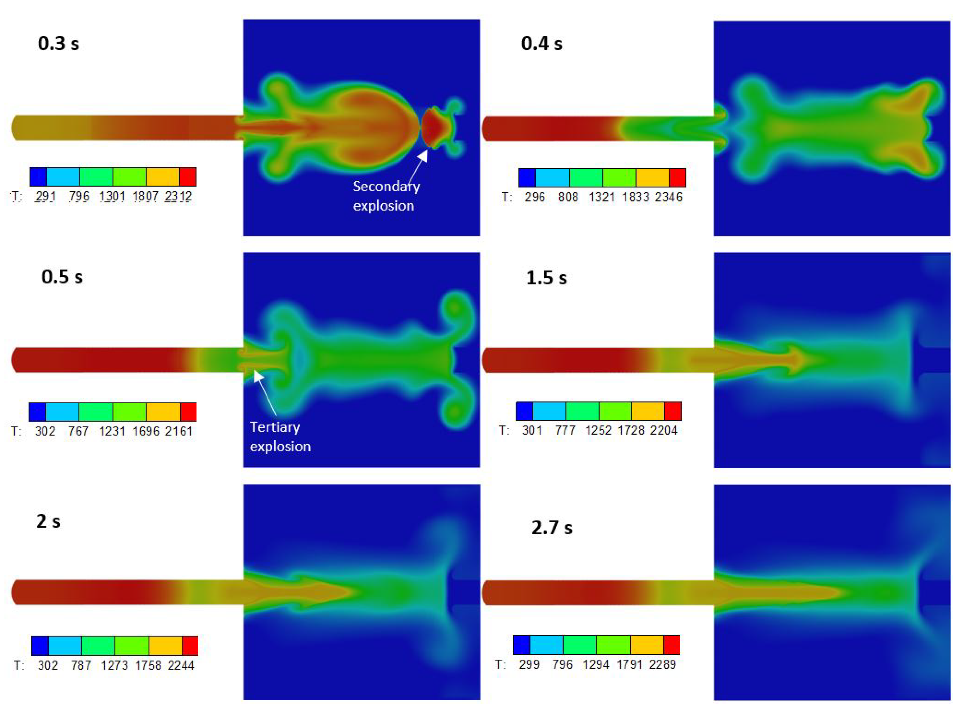
To further confirm the above finding, the scenario with the stoichiometric concentration (i.e., 9.5%) of methane is simulated. The time series of temperature contour for this case (9.5%) is shown in Figure 7. At the stoichiometric condition, the secondary explosion occurs violently inside the evasé even before $t=0.3$ s when the flame ejected from the capture duct is approaching the evasé. Though the flame at the tail of the mushroom still extinguishes due heat loss, the secondary explosion generates strong backflow carrying methane into the capture duct. Due to the high temperature remaining in the capture duct resulted from the first explosion, the tertiary explosion occurs in regions surrounding the mouth of the capture duct at $t=0.5$ s, generating flame propagating against the flame from the secondary explosion. As a result, the space in between the capture duct and the evasé is filled with flame. As methane does not have sufficient time to be completely combusted and is subsequently carried to the region close to the mouth of the capture duct, the tertiary explosion generates flame of even higher temperature. However, as more methane is combusted in regions close to the capture duct mouth, the region of relatively high temperature expands towards the evasé. It should be noted that the tertiary explosion observed in the simulation of this study is for a capture duct length of 30 m, for other capture duct lengths, the occurrence of the tertiary explosion in terms of time and intensity might be different, or it might not occur at all. However, this is out of the interest of the present study. The above results critically confirm that with a distance of $29.4$ m in between the capture duct and evasé, once explosion occurs inside the capture duct with a methane concentration of ≥7.5%, the flame propagates into the evasé and induces the secondary explosion.

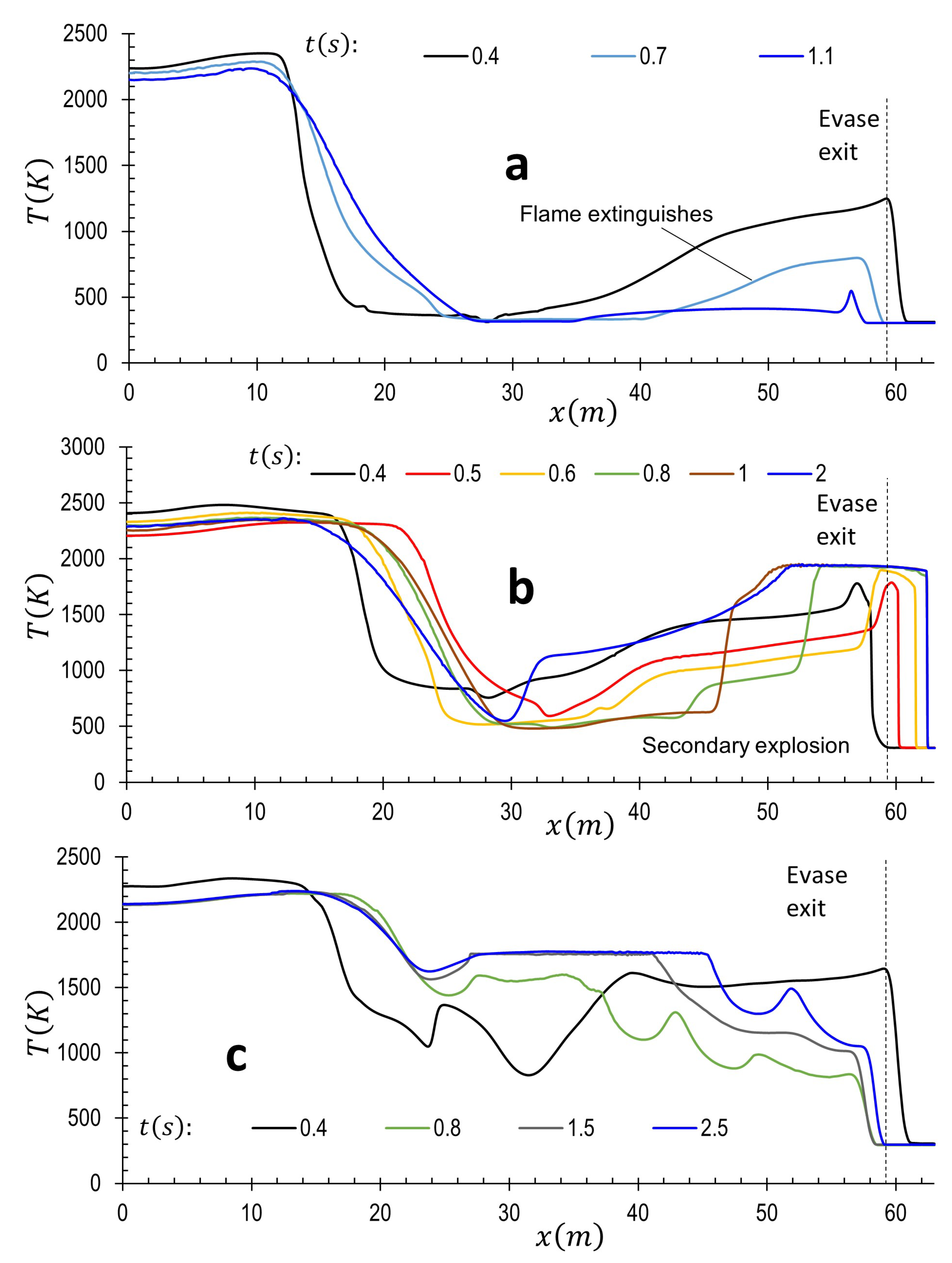
Figure 8 illustrates the quantitative evolution of temperature profile along the centerline for different methane concentrations in the RTO, i.e., 5% (a), 7.5% (b), and 9.5% (c). Distinctly different evolution patterns are observed for these three methane concentrations. Specifically, for the low methane concentration of 5%, Figure 8a, the temperature in the region surrounding the evasé monotonically decreases, indicating the flame extinguishes in this case. For the case with 7.5% methane, Figure 8b, the high temperature (i.e., the flame front generated from the explosion in the capture duct) firstly shifts towards the evasé and induces the secondary explosion inside the evasé that generates a secondary flame propagating outwardly towards the capture duct. After $t=1$ s, a statistically stable flame is formed with an almost constant length and the heated region by the secondary flame expands. For the case with the stoichiometric condition (i.e., 9.5% methane, Figure 8c), the secondary explosion occurs before $t=0.4$ s, the flame propagates backwardly to the capture duct and the burnt gases inside the flame drops due to heat loss to the surroundings, whereas the temperature at the flame front keeps increasing till $t=0.8$ s when the tertiary explosion occurs. From $t=1.5$ s, the temperature of the hot region generated from the tertiary explosion remains constant around $1800K$ with the length increasing towards the evasé.

4. Conclusions

In this study, the flame jump from the capture duct to the evasé was simulated with an air gap of $29.4$ m and different methane concentrations accumulated in the RTO (5–9.5%) representing the extreme flammable conditions of methane.

Once the methane was ignited (in RTO), the spherical laminar flame initiated strong propagation of pressure waves. The rapid reaction process along with sudden changes in local temperature and gas properties led to the alternate cycles of rarefaction and compression of unburnt gases, i.e., the formation of pressure waves. Reflections from the confined tube were observed. The pressure wave magnitude damped inside the capture duct due to energy loss through rarefaction and compression effects. Reflections from the evasé led to bounce-backs of the pressure magnitude at locations in the air gap. Moreover, reflections from the evasé walls caused strong fluctuations of pressure inside the evasé.

After ignition, the laminar flame propagated uniformly outwards. After the flame front reached the tube walls, the statistically spherical flame front geometry transited into a statistically planar geometry and propagated towards the evasé. Due to intrinsic instabilities the planar flame front rapidly changed into a bullet shape.

For the case with 5% methane, the flame that propagated out of the capture duct extinguished at $t=0.7$ s. At $t=1$ s, the temperature around the evasé dropped back to the ambient temperature. For the case of 7.5% methane, secondary explosion was incurred at $t=0.5$ s and at $t=1$ s, a statistically stable flame was formed heating the regions towards the capture duct mouth. With 9.5% methane, the secondary explosion occurred even before the flame reached the evasé. The violent secondary explosion generated strong backflow carrying unburnt fuel backwards and incurred the tertiary explosion at the capture duct mouth. Distinctly different evolution patterns of temperature profiles along the centerline were observed for these three methane concentrations.

The results critically confirm that with an air gap of $29.4$ m between the capture duct and evasé, once explosion occurs inside the RTO where the methane concentration reached 7.5% or above, the flame could incur secondary explosion inside the evasé, which, in turn, could cause explosions in the downstream underground mines.

References

- Pu, G.; Li, X.; Yuan, F. Numerical Study on Heat Transfer Efficiency of Regenerative Thermal Oxidizers with Three Canisters. Processes 2021, 9, 1621. [Google Scholar] [CrossRef]
- Peng, Z.; Doroodchi, E.; Moghtaderi, B. Heat transfer modelling in Discrete Element Method (DEM)-based simulations of thermal processes: Theory and model development. Prog. Energy Combust. Sci. 2020, 79, 100847. [Google Scholar] [CrossRef]
- Sun, S.; Yuan, Z.; Peng, Z.; Moghtaderi, B.; Doroodchi, E. Computational investigation of particle flow characteristics in pressurised dense phase pneumatic conveying systems. Powder Technol. 2018, 329, 241–251. [Google Scholar] [CrossRef]
- Khan, M.S.; Evans, G.M.; Peng, Z.; Doroodchi, E.; Moghtaderi, B.; Joshi, J.B.; Mitra, S. Expansion behaviour of a binary solid-liquid fluidised bed with different solid mass ratio. Adv. Powder Technol. 2017, 28, 3111–3129. [Google Scholar] [CrossRef]
- Peng, Z.; Ge, L.; Moreno-Atanasio, R.; Evans, G.M.; Moghtaderi, B.; Doroodchi, E. VOF-DEM study of solid distribution characteristics in slurry Taylor flow-based multiphase microreactors. Chem. Eng. J. 2020, 396, 124738. [Google Scholar] [CrossRef]
- Peng, Z.; Doroodchi, E.; Evans, G.M. DEM simulation of aggregation of suspended nanoparticles. Powder Technol. 2010, 204, 91–102. [Google Scholar] [CrossRef]
- Chen, J.; Hiu, M.; Chen, Y. Optimizing progress variable definition in flamelet-based dimension reduction in combustion. Appl. Math. Mech. 2015, 36, 1481–1498. [Google Scholar] [CrossRef]
- Piece, C.D. Progress-Variable Approach for Large-Eddy Simulation of Turbulence Combustion. Ph.D Thesis, Stanford University, Stanford, CA, USA, 2001. [Google Scholar]
- van Oijen, J.A.; de Goey, L.P.H. Modelling of premixed laminar flames using Flamelet-Generated Manifolds. Combust. Sci. Technol. 2000, 161, 113–137. [Google Scholar] [CrossRef] [Green Version]
- van Oijen, J.A.; Lammers, F.A.; de Goey, L.P.H. Modeling of complex premixed burner systems by using Flamelet-Generated Manifolds. Combust. Theory Model 2001, 127, 2124–2134. [Google Scholar] [CrossRef]
- van Oijen, J.A.; de Goey, L.P.H. Modelling of premixed counter-flow flames using the flamelet-generated manifold method. Combust. Theory Model 2002, 6, 463–478. [Google Scholar] [CrossRef]
- Akkerman, V.; Bychkov, V.; Petchenko, A.; Eriksson, L.E. Accelerating flames in cylindrical tubes with nonslip at the walls. Combust. Flame 2006, 145, 206–219. [Google Scholar] [CrossRef]
- Peng, Z.; Zanganeh, J.; Ingle, R.; Nakod, P.; Fletcher, D.F.; Moghtaderi, B. Effect of Tube Size on Flame and Pressure Wave Propagation in a Tube Closed at One End: A Numerical Study. Comb. Sci. Technol. 2020, 192, 1731–1753. [Google Scholar] [CrossRef]
- Peng, Z.; Zanganeh, J.; Ingle, R.; Nakod, P.; Fletcher, D.F.; Moghtaderi, B. CFD Investigation of Flame and Pressure Wave Propagation through Variable Concentration Methane-Air Mixtures in a Tube Closed at One End. Comb. Sci. Technol. 2021, 193, 1203–1230. [Google Scholar] [CrossRef]
- Peng, Z.; Zanganeh, J.; Doroodchi, E.; Moghtaderi, B. Flame Propagation and Reflections of Pressure Waves through Fixed Beds of RTO Devices: A CFD Study. Ind. Eng. Chem. Res. 2019, 58, 23389–23404. [Google Scholar] [CrossRef]
- Ajrash, M.J.; Zanganeh, J.; Moghtaderi, B. Deflagration of premixed methane–air in a largescale detonation tube. Process Saf. Environ. 2017, 109, 374–386. [Google Scholar] [CrossRef]
- Ciccarelli, G.; Dorofeev, S. Flame acceleration and transition to detonation in ducts. Prog. Energ. Combust. 2006, 34, 499–550. [Google Scholar] [CrossRef]
- Bychkov, V.; Golberg, S.M.; Liberman, M.A.; Kleev, A.I.; Eriksson, L.E. Numerical simulation of curved flames in cylindrical tubes. Comb. Sci. Technol. 1997, 129, 217–242. [Google Scholar] [CrossRef]
- Pelce-Savornin, C.; Quinard, J.; Searby, G. The flow field of a curved flame propagating freely upwards. Comb. Sci. Technol. 1958, 58, 337–346. [Google Scholar] [CrossRef]
- Clanet, C.; Searby, G. On the “Tulip Flame” Phenomenon. Combust. Flame 1996, 105, 225–238. [Google Scholar] [CrossRef]
Figure 1.
Computational domain and mesh of VAM plant: (a) view and measurements of the computational domain; (b) meshing of the dome section marked as region-I; (c) a close-up view of the mesh of the marked region-II. The flow rate of methane–air mixture released from the evasé () is 180 m/s. In sections 1–3 and the dome section, the stoichiometric methane concentration is present; sections 4–6 and the lower ambient space connecting the capture duct and the evasé are filled with different methane concentrations (5–9.5%), indicated by the different colors.
Figure 2.
Contours of axial pressure (top half) and temperature (bottom half) immediately after igniting the methane–air mixture with 7.5% methane vented from mine.
Figure 3.
Profiles of gas density, temperature, pressure, and axial velocity at ms with 7.5% methane vented from mine.
Figure 4.
Flame development and propagation after ignition of methane–air mixtures inside the capture duct (5% methane).
Figure 5.
Time series of contour of temperature for the scenario where the VAM methane concentration is 5% and the methane ignition/explosion occurs in RTO.
Figure 6.
Time series of the contour of temperature for the scenario where explosion occurs (7.5% methane) in the RTO and generates a flame that propagates out towards the evasé.
Figure 7.
Time series of contour of temperature for the scenario where an explosion occurs in the RTO with 9.5% methane and generates flame that propagates out towards the evasé.
Figure 8.
Time series of temperature profiles after the generated flame in the capture duct reaches the evasé for different methane concentrations in the RTO: (a) 5%; (b) 7.5% and (c) 9.5%.
Publisher’s Note: MDPI stays neutral with regard to jurisdictional claims in published maps and institutional affiliations. |
© 2021 by the authors. Licensee MDPI, Basel, Switzerland. This article is an open access article distributed under the terms and conditions of the Creative Commons Attribution (CC BY) license (https://creativecommons.org/licenses/by/4.0/).
Share and Cite
MDPI and ACS Style
Peng, Z.; Zanganeh, J.; Moghtaderi, B. CFD Modeling of Flame Jump across Air Gap between Evasé and Capture Duct for Ventilation Air Methane Abatement. Processes 2021, 9, 2278. https://0-doi-org.brum.beds.ac.uk/10.3390/pr9122278
AMA Style
Peng Z, Zanganeh J, Moghtaderi B. CFD Modeling of Flame Jump across Air Gap between Evasé and Capture Duct for Ventilation Air Methane Abatement. Processes. 2021; 9(12):2278. https://0-doi-org.brum.beds.ac.uk/10.3390/pr9122278
Chicago/Turabian StylePeng, Zhengbiao, Jafar Zanganeh, and Behdad Moghtaderi. 2021. "CFD Modeling of Flame Jump across Air Gap between Evasé and Capture Duct for Ventilation Air Methane Abatement" Processes 9, no. 12: 2278. https://0-doi-org.brum.beds.ac.uk/10.3390/pr9122278
Note that from the first issue of 2016, this journal uses article numbers instead of page numbers. See further details here.