A Modified Expectation Maximization Approach for Process Data Rectification

Abstract

Process measurements are contaminated by random and/or gross measuring errors, which degenerates performances of data-based strategies for enhancing process performances, such as online optimization and advanced control. Many approaches have been proposed to reduce the influence of measuring errors, among which expectation maximization (EM) is a novel and parameter-free one proposed recently. In this study, we studied the EM approach in detail and argued that the original EM approach is not feasible to rectify measurements contaminated by persistent biases, which is a pitfall of the original EM approach. So, we propose a modified EM approach here to circumvent this pitfall by fixing the standard deviation of random error mode. The modified EM approach was evaluated by several benchmark cases of process data rectification from literatures. The results show advantages of the proposed approach to the original EM in solving efficiency and performance of data rectification.

1. Introduction

With the advancement of smart manufacturing, process measurements play a more and more important role in modern chemical manufacturing plants [1,2,3]. The measurements are unavoidably contaminated by random errors and often by large-sized gross errors, too, which degenerate performances of process monitoring, control and optimization strategies based on measurements [1]. To recover the true values of process variables from the contaminated measurements, many approaches to data rectification, i.e., reducing the random and gross errors simultaneously from the measurements, have been proposed since 1960s [2].

Traditionally, there are three ways of process data rectification, namely, statistical test [4,5], robust estimator [6,7] and mixed integer programming [8,9].

The first way identifies gross errors with a statistical test by assuming random errors follow a normal distribution [10], then a procedure of data reconciliation, i.e., solving a constrained least squares problem whose objective is minimizing the difference between the measured values and reconciled values satisfying process models, is carried out to estimate the true values of the measurements not contaminated by gross errors, while the true values of the measurements contaminated by gross errors are treated as unknown parameters to be estimated. Although the algorithmic parameters, such as critical values of a statistical test, can be chosen with clear statistical meanings, only one gross error can be identified at a time because of the smearing effect of a large-sized gross error, so the approaches of a statistical test must identify gross errors one by one and elegant frameworks must be designed to promise the performance of data rectification [11].

The second way is based on robust estimators [6], which can simultaneously reduce the influences of random and gross errors by solving a constrained nonlinear least squares problem once. Different from the approaches of the statistical test described above, it is assumed that measurements contaminated by random and/or gross errors can be described by a heavy tail statistical distribution, such as contaminated normal [12], Cauchy [6], redescending [13], quasi weighted least squares (QWLS) [14] and correntropy [15] etc., which can effectively reduce the smearing effect of gross errors. The advantages of robust estimators for data rectification are: (1) gross errors can be identified with data reconciliation simultaneously; (2) the parameters of the robust estimators can be determined via Monte Carlo methods with clear statistical meanings [16] or online line search methods based on the Akaike information criterion (AIC) [13]. Currently, the robust estimators may be the most popular approach for process data rectification.

The third way is based on mixed integer programming (MIP) techniques [8,9,10], whose objective is to minimize the number of identified gross errors and the difference between the measured and rectified values, where the trade-off can be realized by the AIC [10,13] or a predetermined weighting factor of the objective function [9,17]. The MIP techniques show competitive or comparable performances to robust estimators for process data rectification, and the MIP technique based on the AIC is free from setting algorithmic parameters to balance the fitness and complexity of the model; although a critical value of identifying gross errors still needs to be determined, this value can be easily obtained from daily operation experiences of instrumentation engineers [10,17].

Recently, a novel way of process data rectification based on statistical inference was proposed, such as the approaches of Bayesian inference [18]. Being a widely used method of statistical inference, expectation maximization (EM) [19,20,21,22,23,24,25] has also been applied to process data rectification [26,27]. The statistical inference approaches are based on the Bayes rule [18], which inferences the unknown parameters by combining the information from collected data (measurements) and the prior probability distribution of the inferenced parameters. Although current works assume prior distribution before process data rectification, some reasonable prior information on the random and gross errors of measurements, such as standard deviation of random errors and occurrence of gross errors for a specified sensor, can be collected and modeled from the experiences of plant operators and historical process data [18,27,28]. So, the authors believe that the statistical inference approach to process data rectification deserves to be studied.

The established EM approach [26] is an interesting statistical inference approach because it has no algorithmic parameter to be determined before data rectification, but just assumes that measurement errors follow a finite Gaussian mixture distribution. The large number of parameters to be estimated with the EM algorithm [29] lead to its low-efficiency solving procedure, and from experiences of the authors, the original EM approach cannot be applied to rectify process measurements contaminated by persistent biases, because the estimated standard deviation of the random error mode is close to that of the gross error mode, which leads to difficulty of bias identification.

In this work, we argue that, for the original EM approach, the estimated value of standard deviation of random error mode is unavoidably enlarged by a persistent bias and leads to difficulty of bias detection. To circumvent this problem, we present a modified EM approach, where the standard deviation of random error mode is estimated before the EM iterations with a robust method [30], so the standard deviation of random error mode will not be enlarged by a persistent bias and it is possible to detect bias from the EM calculation result. Compared to the original EM approach, the modified one also reduces the number of parameters to be estimated and the time consumption of EM iterations can also be significantly reduced.

The remainder of this paper is organized as follows. Section 2 introduces the principles of the established EM approach for data rectification. The proposed modified EM approach and detailed calculation steps are presented in Section 3. Section 4 describes the performance analysis procedure used herein. The performance modified EM approach is evaluated and compared to the original one in Section 5. Finally, Section 6 concludes the paper.

2. Data Rectification Approach of Expectation Maximization

2.1. Data Rectification Problem

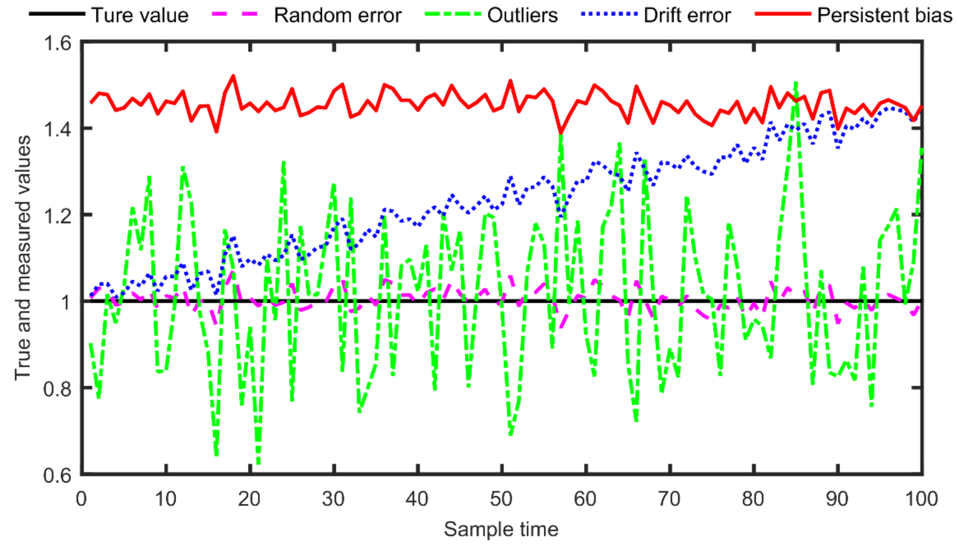
Except for the random errors following normal distribution, three types of gross errors, namely, drift, outlier and persistent bias, also usually contaminate measurements, which are shown in the following Figure 1.

Figure 1 shows how different types of gross errors contaminate a process measurement whose true value is 1 in steady state. Obviously, any one of the systematic errors significantly reduces the reliability of a process measurement, which is the basis of online decision-making during the enhancement of the process performance and a systematic error cannot be eliminated with data reconciliation methods, because a zero mean of random error is assumed for the methods of data reconciliation. Essentially, outliers in a measurement horizon are also random errors with larger variance than random noises, and the original EM algorithm can identify and estimate outliers well. A persistent bias as shown in Figure 1 is not random, which will enlarge the estimated variance of the original EM algorithm, as shown in the following Section 3.1. On drift error of a sensor, it is also a non-random one with increasing error size and it will also lead to an enlarged estimated variance as a persistent error, supposing an average of a measurement horizon is taken as a representative of the horizon. In the following, we show how a data rectification problem is set up as a statistical inference problem.

Supposing a measurement horizon ${\left\{y_{j,h}\right\}}_{h=t-H+1}^t$ is collected at time t, which involves H data points measured at different time point k for the jth process variable and a data matrix $Y\in R^{J\times H}$ whose rows represent measurement horizons of all the J measured process variables, where $y_{j,h}$ is an element at the jth row and hth column of Y. A steady-state process data rectification can be formulated as a maximum likelihood estimation problem described as the following Equation (1).

$$\begin{array}{l}\underset{x}{\max }\ln \left[P\left(Y|x\right)\right]\\ s.t.\left\{\begin{array}{c}f\left(x\right)=0\\ g\left(x\right)\le 0\end{array}\right.\end{array}$$

(1)

In Equation (1), the objective function is the logarithm likelihood of the sampled measurements $y_{j,h}$ under the condition that the true value of the jth measurement is $x_j$ and the jth element of vector x is $x_j$; f (x) represents the process model and g(x) denotes the inequality constraints for the process variables, considering operational specifications and experienced bounds.

Assuming different distributions of the measurement errors, the formulation of the objective function of Equation (1) varies [6]. For the data reconciliation problem considering random errors only, it is assumed that random errors follow a normal distribution, and the logarithm of the objective function is a quadratic one. If a heavy tail distribution is assumed for measurement errors, as in the situation of data rectification using robust estimators, the logarithm of the objective function shows a more complex formulation, sometimes the function is nonconvex or even discontinuous [6].

In both the situations described above, we fix the distribution parameters of measurement errors. For the data rectification using the EM approach, the parameters of measurement error distribution are inferenced with the Bayes rule, as described in the following section.

2.2. Expectation Maximization Approach

For the EM approach [26], the difference between the hth measurement and the true value of the jth process variable, namely, ${\epsilon }_{j,h}=y_{j,h}-x_j$, is described with the finite Gaussian mixture model shown with Equation (2) [26].

$$\begin{array}{l}{\epsilon }_{j,h}=y_{j,h}-x_j=w_{j,1}N\left(0,{\sigma }_{j,1}^2\right)+w_{j,2}N\left(0,{\sigma }_{j,2}^2\right)\\ s.t.\left\{\begin{array}{c}{w}_{j,1},w_{j,2}\ge 0\\ w_{j,1}+w_{j,2}=1\end{array}\right.\end{array}$$

(2)

In Equation (2), $w_{j,1}$ represents the probability of a random error mode with a zero mean and standard deviation ${\sigma }_{j,1}$, and $w_{j,2}$ represents the probability of a gross error mode with a zero mean and standard deviation ${\sigma }_{j,2}$ that is larger than ${\sigma }_{j,1}$ under the occurrence of a gross error. Supposing ${\theta }_j={\left\{{\sigma }_{j,k},w_{j,k}\right\}}_{k=1,2}$, the likelihood of ${\epsilon }_{j,h}$ for the kth error mode can be described with the following Equation (3) [26].

$$p_{j,h,k}=P\left(y_{j,h}|z_{j,h}=k,x_j,{\theta }_j\right)=\frac{1}{\sqrt{2\pi {\sigma }_{j,k}^2}}\exp \left[-\frac{{\left(y_{j,h}-x_j\right)}^2}{{\sigma }_{j,k}^2}\right]$$

(3)

In Equation (3), $z_{j,h}$ is a latent variable to be estimated and $z_{j,h}=k$ represents that the error mode of $y_{j,h}$ is the kth one, where k = 1 represents a random error mode, and k = 2 means a gross error mode. Considering both error modes, the whole likelihood of ${\epsilon }_{j,h}$ is represented as following Equation (4).

$$p_{j,h}={\displaystyle \sum _{k=1}^2{w}_{j,k}{p}_{j,h,k}}$$

(4)

Based on the above descriptions, the previously mentioned Equation (1) can be written as the following Equation (5).

$$\begin{array}{l}\underset{x_j,{\theta }_j}{\max }\ln \left[{\displaystyle \prod _{j=1}^J{\displaystyle \prod _{h=1}^H{p}_{j,h}}}\right]\\ s.t.\left\{\begin{array}{c}f\left(x\right)=0\\ g\left(x\right)\le 0\end{array}\right.\end{array}$$

(5)

It is difficult to solve Equation (5) directly, because $w_{j,k}$ cannot be obtained explicitly. Hence, an EM approach was applied to solve Equation (5), by replacing Equation (5) with the following Equation (6) [26].

$$\begin{array}{ll}\underset{\Theta }{\max }Q\left(\Theta ,{\Theta }^{\left(t\right)}\right)& =E_{z_{j,h}=k|y_{j,h},{\Theta }^{\left(t\right)}}\left[\ln {\displaystyle \prod _{j=1}^J{\displaystyle \prod _{h=1}^{H}p\left(z_{j,h}=k,y_{j,h}|\Theta \right)}}\right]\\ & ={\displaystyle \sum _{j=1}^J{\displaystyle \sum _{h=1}^H{E}_{z_{j,h}=k|y_{j,h},{\Theta }^{\left(t\right)}}\ln p\left(z_{j,h}=k,y_{j,h}|\Theta \right)}}\\ & ={\displaystyle \sum _{j=1}^J{\displaystyle \sum _{h=1}^H{\displaystyle \sum _{k=1}^{2}p\left(z_{j,h}=k|y_{j,h},{\Theta }^{\left(t\right)}\right)\cdot \ln p\left(z_{j,h}=k,y_{j,h}|\Theta \right)}}}\\ s.t.\left\{\begin{array}{c}f\left(x\right)=0\\ g\left(x\right)\le 0\end{array}\right.& \end{array}$$

(6)

In Equation (6), $\Theta ={\left\{x_j,{\theta }_j\right\}}_{j=1,\dots J}$ and ${\Theta }^{\left(t\right)}$ represent the estimation result of $\Theta$ at the tth iteration, which means the probability of error mode for a measurement, namely, $p\left(z_{j,h}=k|y_{j,h},{\Theta }^{\left(t\right)}\right)$, is estimated from $y_{j,h}$ and ${\Theta }^{\left(t\right)}$ using the Bayes rule, as described with Equation (7).

$$\begin{array}{ll}P\left(z_{j,h}=k|y_{j,h},{\Theta }^{\left(t\right)}\right)& =\frac{P\left(z_{j,h}=k,y_{j,h},{\Theta }^{\left(t\right)}\right)}{P\left(y_{j,h},{\Theta }^{\left(t\right)}\right)}\\ & =\frac{P\left(y_{j,h},z_{j,h}=k,{\Theta }^{\left(t\right)}\right)}{P\left(y_{j,h},{\Theta }^{\left(t\right)}\right)}\\ & =\frac{P\left(y_{j,h}|z_{j,h}=k,{\Theta }^{\left(t\right)}\right)\cdot P\left(z_{j,h}=k,{\Theta }^{\left(t\right)}\right)}{P\left(y_{j,h},{\Theta }^{\left(t\right)}\right)}\\ & =\frac{P\left(y_{j,h}|z_{j,h}=k,{\Theta }^{\left(t\right)}\right)\cdot P\left(z_{j,h}=k,{\Theta }^{\left(t\right)}\right)}{P\left(y_{j,h},{\Theta }^{\left(t\right)}\right)}\\ & =\frac{P\left(y_{j,h}|z_{j,h}=k,{\Theta }^{\left(t\right)}\right)\cdot P\left(z_{j,h}=k|{\Theta }^{\left(t\right)}\right)\cdot P\left({\Theta }^{\left(t\right)}\right)}{P\left(y_{j,h}|{\Theta }^{\left(t\right)}\right)\cdot P\left({\Theta }^{\left(t\right)}\right)}\\ & =\frac{P\left(y_{j,h}|z_{j,h}=k,{\Theta }^{\left(t\right)}\right)\cdot P\left(z_{j,h}=k|{\Theta }^{\left(t\right)}\right)}{P\left(y_{j,h}|{\Theta }^{\left(t\right)}\right)}\\ & =\frac{p_{j,h,k}\cdot w_{j,k}}{{\displaystyle \sum _{l=1}^2{p}_{j,h,l}\cdot w_{j,l}}}\end{array}$$

(7)

In Equation (7), $p_{j,h,k}$ is calculated with Equation (3) and $P\left(z_{j,h}=k|{\Theta }^{\left(t\right)}\right)=w_{j,k}$ because $\mathsf{\Theta }={\left\{x_j,{\theta }_j\right\}}_{j=1,\dots J}$ and ${\theta }_j={\left\{{\sigma }_{j,k},w_{j,k}\right\}}_{k=1,2}$. The calculation of the probability of $P\left(z_{j,h}=k|y_{j,h},{\Theta }^{\left(t\right)}\right)$ is noted as the expectation step (E-step).

After the E-step, we estimate $\mathsf{\Theta }$ using the maximization step (M-step), namely, solving Equation (6) with fixed $P\left(z_{j,h}=k|y_{j,h},{\Theta }^{\left(t\right)}\right)$ calculated at the E-step, then a new estimation of $\mathsf{\Theta }$, i.e., ${\mathsf{\Theta }}^{\left(t+1\right)}$, is the result. It must be noted that $\ln p\left(z_{j,h}=k,y_{j,h}|\mathsf{\Theta }\right)$ is calculated with Equation (3) and the Bayes rule, as described by Equation (8).

$$\begin{array}{ll}\ln p\left(y_{j,h},z_{j,h}=k|\mathsf{\Theta }\right)& =\ln \left[\frac{p\left(y_{j,h},z_{j,h},\mathsf{\Theta }\right)}{p\left(\mathsf{\Theta }\right)}\right]\\ & =\ln \left[\frac{p\left(y_{j,h}|z_{j,h},\mathsf{\Theta }\right)\cdot p\left(z_{j,h},\mathsf{\Theta }\right)}{p\left(\mathsf{\Theta }\right)}\right]\\ & =\ln \left[p\left(y_{j,h}|z_{j,h},\mathsf{\Theta }\right)\cdot p\left(z_{j,h}|\mathsf{\Theta }\right)\right]\\ & =\ln p_{j,h,k}+\ln \left[p\left(z_{j,h}|\mathsf{\Theta }\right)\right]\\ & =-\ln \left(\sqrt{2\pi }{\sigma }_{j,k}\right)-{\left(\frac{y_{j,h}-x_j}{{\sigma }_{j,k}}\right)}^2+\ln w_{j,k}\end{array}$$

(8)

To solve Equation (6), a coordinate search method is applied to estimate $w_{j,k}$ and ${\sigma }_{j,k}$ separately, as the following Equations (9) and (10) show [26].

$${\sigma }_{j,k}^{\left(t+1\right)}=\sqrt{\frac{{\displaystyle \sum _{h=1}^H{\gamma }_{j,h,k}^{\left(t\right)}\cdot {\left(y_{j,h}-x_j^{\left(t\right)}\right)}^2}}{{\displaystyle \sum _{h=1}^H{\gamma }_{j,h,k}^{\left(t\right)}}}},$$

(9)

$$w_{j,k}^{\left(t+1\right)}=\frac{{\displaystyle \sum _{j=1}^H{\gamma }_{j,h,k}^{\left(t\right)}}}{H}.$$

(10)

In the above equations, ${\gamma }_{j,h,k}^{\left(t\right)}=P\left(z_{j,h}=k|y_{j,h},{\mathsf{\Theta }}^{\left(t\right)}\right)$, which is calculated with Equation (7). At last, $x_j^{\left(t+1\right)}$ is estimated by solving Equation (6) with $w_{j,k}$ and ${\sigma }_{j,k}$ fixed as Equations (9) and (10) [26].

With the new estimation of $\mathsf{\Theta }$, i.e., ${\mathsf{\Theta }}^{\left(t+1\right)}$, obtained, we return to the E-step and check the difference between $Q\left(\mathsf{\Theta },{\mathsf{\Theta }}^{\left(t\right)}\right)$ and $Q\left(\mathsf{\Theta },{\mathsf{\Theta }}^{\left(t+1\right)}\right)$ of Equation (6), if the difference is not obvious we stop the iteration, or the else we continue [26].

3. Modified Expectation Maximization Approach

3.1. Standard Deviation of the Original EM under Persistent Bias

Although the EM approach was successfully applied to several situations, such as non-persistent gross errors and concurrent errors of different types [26,27], there is still a little space for improvement in the situation of measurements contaminated by persistent biases, where ${\left(y_{j,h}-x_j^{\left(t\right)}\right)}^2$ in Equation (9) is relatively large and unavoidably leads to a large ${\sigma }_{j,k}^{\left(t+1\right)}$ even for the random error mode, whose standard deviation shall be relatively small, as can be argued in the follows.

Supposing that ${\alpha }_{j,h,k}={\gamma }_{j,h,k}^{\left(t\right)}/{\displaystyle \sum _{h=1}^H{\gamma }_{j,h,k}^{\left(t\right)}}$, Equation (9) can be rewritten as following Equation (11):

$${\left[{\sigma }_{j,k}^{\left(t+1\right)}\right]}^2={\displaystyle \sum _{h=1}^H{\alpha }_{j,h,k}\cdot {\left(y_{j,h}-x_j^{\left(t\right)}\right)}^2},{\alpha }_{j,h,k}\in \left[0,1\right]\mathrm{and}{\displaystyle \sum _{h=1}^H{\alpha }_{j,h,k}}=1$$

(11)

With $h^{\prime }=\underset{h}{\arg \min }\left\{{\left(y_{j,h}-x_j^{\left(t\right)}\right)}^2\right\}$ and ${\alpha }_{j,h^{\prime },k}=1$, it is easy to infer that Equation (11) arrived at its minimum, namely, ${\left[{\sigma }_{j,k}^{\left(t+1\right)}\right]}_{\min }={\left|y_{j,h}-x_j^{\left(t\right)}\right|}_{\min }$, which fluctuates around the magnitude of the bias contaminating the jth measurement and leads to a large size standard deviation for random error mode of Equation (2), namely, ${\sigma }_{j,1}$. Under this situation, it is impossible to set $\pm 3{\sigma }_{j,1}$ as the critical value for bias detection and the original intention of Equation (2) is violated, too.

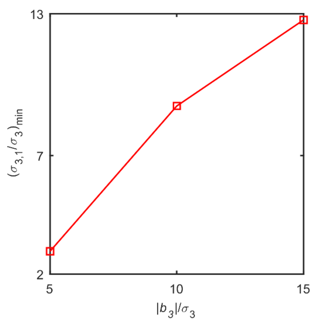
To verify the above argument, the simple linear data rectification case of Ripps [31] is used here to show the influence of persistent bias to the standard deviations of random mode. The Ripps case involves four streams with measured flowrates and three linear mass balance equality constraints are shown as the following Equation (12).

$$\left\{\begin{array}{c}0.1x{}_1+0.6x_2-0.2x_3-0.7x_4=0\\ 0.8x{}_1+0.1x_2-0.2x_3-0.1x_4=0\\ 0.1x{}_1+0.3x_2-0.6x_3-0.2x_4=0\end{array}\right.$$

(12)

The true values of all the flowrates are $x{}_1$ = 0.1739, $x{}_2$ = 5.0435, $x{}_3$ = 1.2175 and $x{}_4$ = 4, with corresponding standard deviations ${\sigma }_1$ = 2.89 × 10⁻⁴, ${\sigma }_2$ = 2.5 × 10⁻³, ${\sigma }_3$ = 5.76 × 10⁻⁴, and ${\sigma }_4$ = 4 × 10⁻² for random noises. Here we assume that $x_3$ is contaminated by a bias with sizes being 5${\sigma }_3$, 10${\sigma }_3$ and 15${\sigma }_3$, respectively, then 50 Monte Carlo simulations are carried for each bias size, with all the variables being added random noises with zero mean and corresponding standard deviations. For each Monte Carlo simulation, the sign of the bias is assigned randomly with equal probability. The minimum ratio of estimated ${\sigma }_{3,1}$ to ${\sigma }_3$, namely, ${\left(\frac{{\sigma }_{3,1}}{{\sigma }_3}\right)}_{\min }$, is shown in Figure 2 as follows.

As Figure 2 shows, as in the above argument, the minimum estimated standard deviation of random noise mode is several times of that of the true, so it is impossible to detect a bias with the traditional 3 σ rule, as the original EM approach did [26].

3.2. Modification to the Original EM Approach

To apply the EM approach to the situation of measurements contaminated by persistent biases, a simple modification is presented herein for the original EM approach, namely, we directly estimate the variance of the random error mode in Equation (2), i.e., ${\sigma }_{j,1}^2$, but not via the EM iterations. It has been shown that ${\sigma }_{j,1}^2$ can be estimated efficiently and robustly from process measurements even when the measurements are contaminated with gross errors [30]. Then all the other parameters of $\mathsf{\Theta }$ in Equation (6) are still estimated using the above original EM procedure. Obviously, the influence of bias on the estimation of standard deviation of random error is avoided by this modification.

After $\mathsf{\Theta }$ in Equation (6) being estimated, a criterion must be set up to detect bias for measurements. There are two established ways for detecting bias. The first one is shown by Equation (13), namely, a measurement is contaminated by a bias if the probability of gross error mode is larger than the random error mode [12]. The second one is using the deviation of reconciled value from the corresponding measured value [26], namely, if the following Equation (14) holds where ${\overline{y}}_j$ is the average of measurement horizon of the jth process variable, then a bias is detected for the jth measured variable.

$$w_{j,2}{\displaystyle \sum _{h=1}^H\frac{1}{\sqrt{2\pi {\sigma }_{j,2}^2}}\exp \left[-\frac{{\left(y_{j,h}-x_j\right)}^2}{{\sigma }_{j,2}^2}\right]}>w_{j,1}{\displaystyle \sum _{h=1}^H\frac{1}{\sqrt{2\pi {\sigma }_{j,1}^2}}\exp \left[-\frac{{\left(y_{j,h}-x_j\right)}^2}{{\sigma }_{j,1}^2}\right]},$$

(13)

$$\left|{\overline{y}}_j-x_j\right|>3{\sigma }_{j,1}.$$

(14)

Obviously, the original EM approach can only use the first way of bias detection because the estimated value of ${\sigma }_{j,1}$ is enlarged by a persistent bias. While three criteria can be applied to the modified EM approach, i.e., a bias is detected when Equation (13) holds, which is noted as probability criterion (PC); or Equation (14) holds, which is noted as deviation criterion (DC); or both Equations (13) and (14) hold simultaneously, which is noted as a probability and deviation criterion (PDC).

Based on the above description, the proposed modified EM approach can be shown in

Table 1. Modified expectation maximization (EM) approach for data rectification.

1. Input measurements matrix Y.

2. Estimate ${\sigma }_{j,1}^2$ from Y by using a robust direct approach [30].

3. Initialize parameters: $w_{j,1}^{\left(0\right)}=0.5,{\sigma }_{j,2}^{\left(0\right)}={\sigma }_{j,1},x_j^{\left(0\right)}={\displaystyle \sum _{h=1}^H{y}_{j,h}}/H$ and set t = 1.

4. E-step. Calculate $P\left(z_{j,h}=k|y_{j,h},{\Theta }^{\left(t\right)}\right)$ using Equation (7).

5. M-step. Calculate ${\sigma }_{j,2}^{\left(t+1\right)}$ and $w_{j,k}^{\left(t+1\right)}$ using Equations (9) and (10), respectively, calculate $x_j^{\left(t+1\right)}$ by solving Equation (6) with ${\sigma }_{j,2}={\sigma }_{j,2}^{\left(t+1\right)}$ and $w_{j,k}=w_{j,k}^{\left(t+1\right)}$ fixed.

6. Terminate if $\left|\left[Q\left(\Theta ,{\Theta }^{\left(t+1\right)}\right)-Q\left(\Theta ,{\Theta }^{\left(t\right)}\right)\right]/Q\left(\Theta ,{\Theta }^{\left(t\right)}\right)\right|\le {10}^{-3}$, or else t = t + 1 and return to step 4.

7. Detect bias for each measurement with PC, DC or PDC.

.

The modified EM with PC, DC or PDC for bias detection is noted as MEM-PC, EM-DC and EM-PDC, respectively.

The advantages of the modified EM algorithm over the original EM algorithm are: (1) the standard deviation of random error is not affected by a persistent bias, because a direct and robust variance estimation method [30] is used; (2) fewer variables need to be estimated by the modified EM algorithm, which means that the modified EM algorithm converges faster than the original EM algorithm.

4. Performance Analysis

To evaluate the performance of the proposed modified EM algorithm, the following three performance metrics, namely, overall performance (OP), average number of Type-I error (AVTI) and relative error reduction (RER), defined as following Equations (15)–(19) are used here [9].

$$\mathrm{OP}=\frac{\mathrm{number}\mathrm{of}\mathrm{correctly}\mathrm{identified}\mathrm{bias}}{\mathrm{number}\mathrm{of}\mathrm{gross}\mathrm{errors}\mathrm{simulated}},$$

(15)

$$\mathrm{AVTI}=\frac{\mathrm{number}\mathrm{of}\mathrm{wrongly}\mathrm{identified}\mathrm{bias}}{\mathrm{number}\mathrm{of}\mathrm{simulation}\mathrm{trials}},$$

(16)

$$\mathrm{RER}=\frac{{\displaystyle \sum _{j=1}^M\left(MR{E}_j-RR{E}_j\right)}}{{\displaystyle \sum _{j=1}^{M}MR{E}_j}},$$

(17)

$$MR{E}_j=\left|\frac{{\overline{x}}_j-x_j^t}{x_j^t}\right|,$$

(18)

$$RR{E}_j=\left|\frac{x_j-x_j^t}{x_j^t}\right|.$$

(19)

The following Monte Carlo simulation procedure [6] is carried here to evaluate the performance of data rectification.

(1)

For all the measured variables, add random noises with zero mean and corresponding standard deviation.

(2)

Add bias to each measurement with a predefined probability p_b, the bias size randomly distributes in the range of 5 and 25 times of standard deviation of random noise, the sign of the bias, namely, ‘+’ or ‘−‘, is randomly assigned with equal probability.

(3)

Calculate performance of data rectification with Equations (15)–(19) for each evaluated method.

Four well-known test cases of process data rectification were used here to evaluate and compare the performances of the proposed MEM approach to the original EM approach, which are described as following.

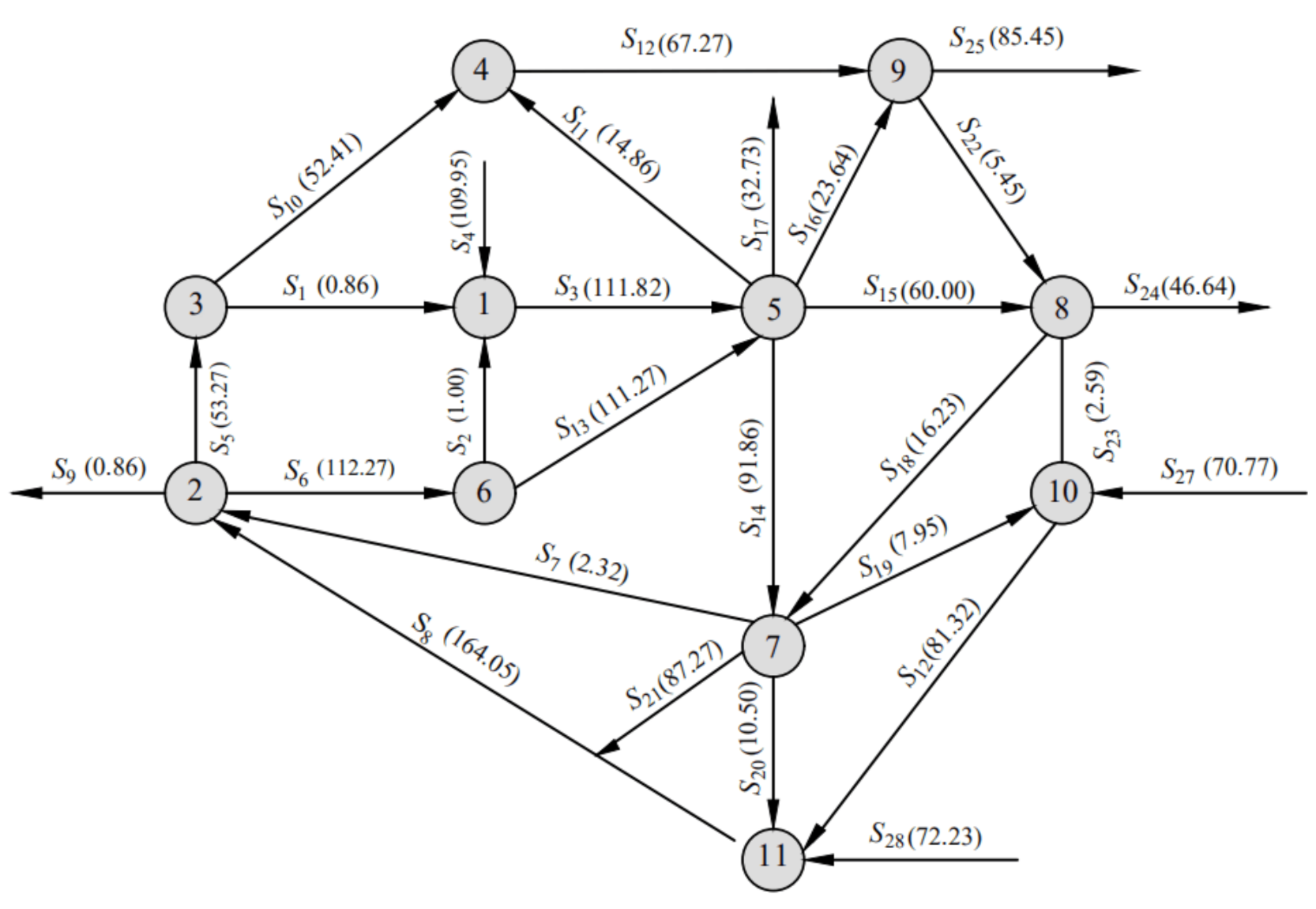
The first case is the famous steam metering network (SMN) [32], which involves 11 units interconnected by 28 streams with measured flow rates, whose flowsheet diagram is demonstrated as Figure 3 with the true values of the flowrates of all the streams shown in the parenthesis. For each measured variable, the standard deviation of added random noise is set as 2.5% of its true values.

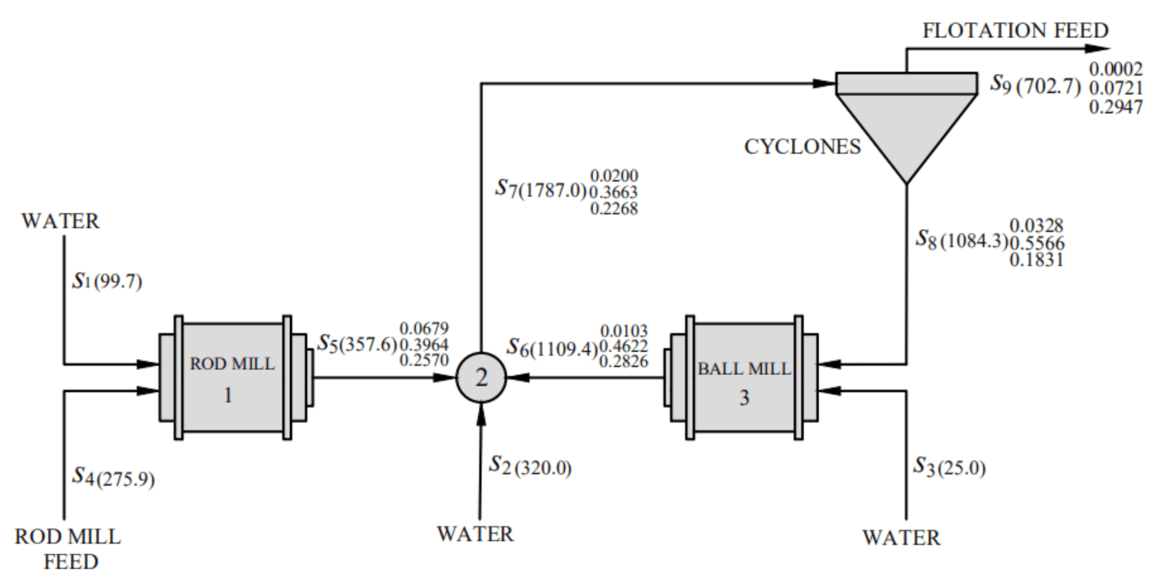
The second case is a bilinear process of metallurgical grinding (MG) [33], which involves four units interconnected by nine streams with measured mass flowrates and 15 measured mass fractions. The flowsheet of the metallurgical grinding is shown in Figure 4 with the true values of all the measured variables, where the true values of flowrates are shown in the parenthesis and composition shown at the right side of the parenthesis. For all the measured variables, the corresponding $\sigma$ of random noise is set as 2.5% of its true value.

The third case, i.e., Pai-Fisher (PF) [34], is a typical nonlinear instance of data rectification, whose model is shown as the following Equation (20). The true values of the measured variables are x = [4.5124; 5.5819; 1.9260; 1.4560; 4.8545] and true values of unmeasured variables are v = [11.070; 0.61467; 2.0504]. For all the measured variables, the corresponding $\sigma$ of random noise is set as 2.5% of its true value.

$$\left\{\begin{array}{l}0.5x_1^2-0.7x_2+x_3{v}_1+v_1{v}_2{x}_2^2+2x_3{v}_3^2=255.8\hfill \\ x_1-2x_2+3x_1{x}_3-2x_2{v}_1-x_2{v}_2{v}_3=-111.2\hfill \\ x_3{v}_1-x_1+3x_2+x_1{v}_2-x_3{v}_3^{0.5}=33.57\hfill \\ x_4-x_1-x_3^2+v_2+3v_3=0\hfill \\ x_5-2x_3{v}_2{v}_3=0\hfill \\ 2x_1+x_2{x}_3{v}_1+v_2-v_3=126.6\hfill \end{array}\right.$$

(20)

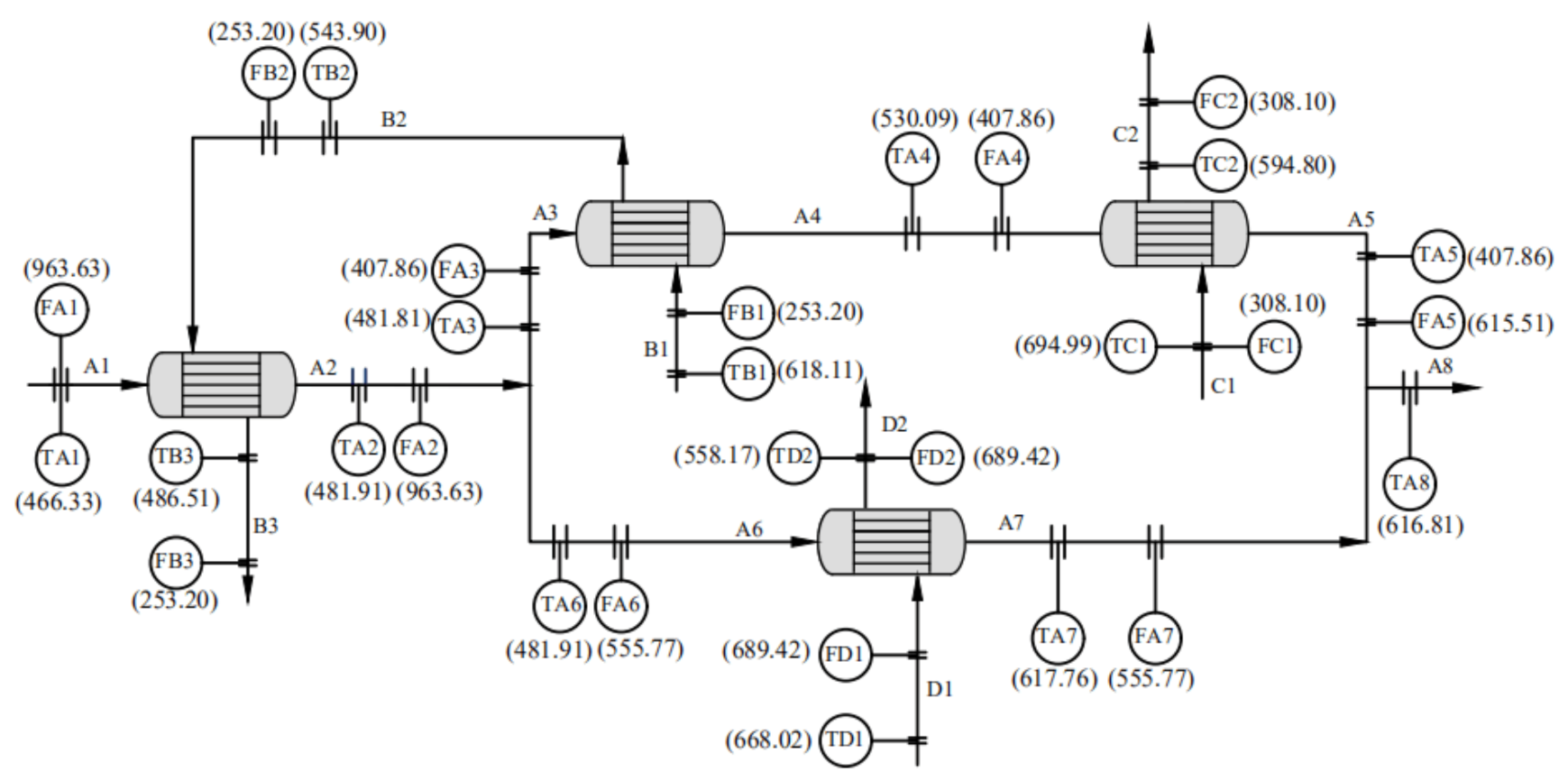
The fourth case, namely, the Swartz case (Sw) [35], is a heat exchanger network, where streams Ai (i = 1, 2, …, 8) is heated by streams Bi (i = 1,2,3), Ci (i = 1,2) and Di (i = 1,2) via different heat exchangers, as Figure 5 shows. The true values of flowrate and temperature for each stream [12] are shown in Figure 5, too. The standard deviation of random noise for each flowrate is set as 2.5% of the corresponding true value of flowrate and 0.75 for temperature of each stream.

For the Swartz case, both linear material balance equalities and nonlinear energy balance equalities for each heat exchanger/junction are used as constraints of data rectification. The enthalpy of unit mass of each stream is correlated with its temperature using a quadratic polynomial as Equation (21) shows, whose coefficients are shown in

Table 2. Coefficients of temperature-enthalpy correlation for each stream.

Stream	Ai (i = 1, 2, …, 8)	Bi (i = 1, 2, 3)	Ci (i = 1, 2)	Di (i = 1, 2)
v1	−6.8909	−14.8538	−28.2807	−11.4172
v2	0.0991	0.1333	0.1385	0.1229
v3	1.1081 × 10−4	7.539 × 10−5	9.043 × 10−5	7.94 × 10−5

[1].

$$H=v_1+v_{2}T+v_3{T}^2$$

(21)

For all the tested cases, the Monte Carlo simulations were carried out in a MATLAB 2018 (MathWorks, Boston, MA, USA) environment using a personal computer with Intel Core Processor (TM) i3 CPU 3120M @ 2.50 GHz, 8GB RAM (Intel, Santa Clara, CA, USA), random measuring noises were generated by “normrnd” command and “rand” command was used to assign the size and sign of a bias. The nonlinear programs of the EM were solved with “fmincon” command.

5. Results and Discussion

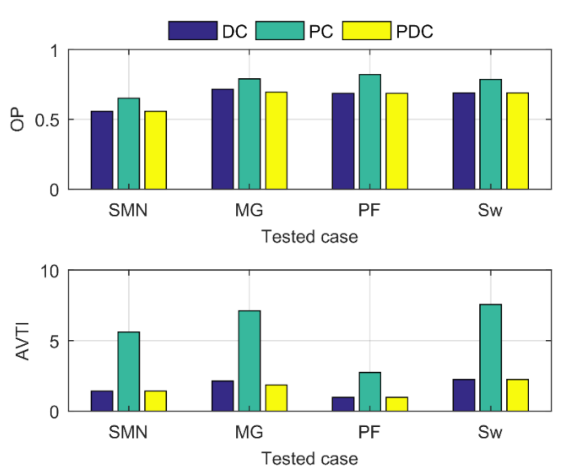
To evaluate the performances of different criteria of the modified EM approach, the OP and AVTI performances of the DC, PC and PDC for all the four tested cases are compared as shown in Figure 6.

As Figure 6 shows, PC had higher OP and obviously higher AVTI than DC and PDC, which shows that the probabilities of random and gross error modes are not feasible to detect a bias because some variables not contaminated by a bias also have higher probability of gross error mode. The DC and PDC had the same OP and AVTI except for the bilinear MG case, where PDC detected a little less bias than DC; whether this was a special case needs to be investigated in the future, since this work focuses on modifying the original EM approach for rectifying measurements contaminated by persistent biases.

Because MEM-DC and MEM-PDC had almost the same performances of data rectification, MEM-DC was selected to be compared to the original EM approach, as shown in

Table 3. The performances of the original and modified EM approaches for the tested cases.

Case	Total Biases	Method	OP	AVTI	RER	Time (s)
SMN	6984	EM	0.1668	3.0030	0.3542	8.3979
		MEM-DC	0.5488	1.4330	0.3628	1.0425
Grinding	6061	EM	0.2153	3.0980	0.4489	7.4701
		MEM-DC	0.6976	1.6590	0.4578	2.0415
Pai-Fisher	1213	EM	0.2003	0.9990	0.4804	0.6180
		MEM-DC	0.6735	1.0200	0.4838	0.5719
Swartz	2564	EM	0.1998	5.4910	0.7348	7.0294
		MEM-DC	0.6895	2.2480	0.7388	0.7423

. As stated in Section 3.2, PC was used to detect bias for the original EM, because DC does not work in the situation of persistent bias contaminating measurement, the standard deviation of random mode, i.e., ${\sigma }_{j,1}$, was enlarged by the bias contaminating the jth measurement, as shown in Figure 1, and DC based on the 3$\sigma$ rule cannot detect any bias from experiences of the authors.

As Table 3 shows, the original EM had much lower OP and much higher AVTI than MEM-DC, which shows that the persistent bias influences not only the standard deviation of random error mode, but also the probability of random and gross error modes. It is interesting that the original EM approach had only a little worse RER than MEM-DC, which shows that the rectified values of both approaches are close to each other. At last, MEM-DC obviously consumed much less time than the original EM, because fewer parameters needed to be estimated for the former one.

6. Conclusions

In this work, we analyze the influence of a persistent bias on the estimated standard deviation of the random error mode for the EM approach and argue that the 3$\sigma$ rule cannot be used to detect bias under the occurrence of a persistent bias. A modified EM approach was devised by estimating the standard deviation of random error mode from process measurements before the EM iterations. The performances of the modified and original EM approaches were evaluated and compared through four widely used linear and nonlinear examples of data rectification, and the results show that the original EM approach cannot be used to detect persistent biases, while the modified EM can; the modified EM consumes much less time than the original EM due to the reduction of estimated parameters.

The convergence of the modified EM algorithm is not proved and we will study this in the future to increase our understanding of the EM approach and to increase the reliability of the proposed EM approach.

References

- Valle, E.; Kalid, R.; Secchi, A.; Kiperstok, A. Collection of Benchmark Test Problems for Data Reconciliation and Gross Error Detection and Identification. Comput. Chem. Eng. 2018, 111, 134–148. [Google Scholar] [CrossRef]
- de Menezes, D.Q.F.; de Sá, M.C.C.; Fontoura, T.B.; Anzai, T.K.; Diehl, F.C.; Thompson, P.H.; Pinto, J.C. Modeling of Spiral Wound Membranes for Gas Separations—Part II: Data Reconciliation for Online Monitoring. Processes 2020, 8, 1035. [Google Scholar] [CrossRef]
- Qian, F.; Zhong, W.; Du, W. Fundamental Theories and Key Technologies for Smart and Optimal Manufacturing in the Process Industry. Engineering 2017, 3, 154–160. [Google Scholar] [CrossRef]
- Crowe, C.M. Data Reconciliation—Progress and Challenges. J. Proc. Cont. 1996, 6, 89–98. [Google Scholar] [CrossRef]
- Guo, S.; Liu, P.; Li, Z. Data Reconciliation for the Overall Thermal System of a Steam Turbine Power Plant. Appl. Energy 2016, 165, 1037–1051. [Google Scholar] [CrossRef]
- Özyurt, D.; Pike, R. Theory and Practice of Simultaneous Data Reconciliation and Gross Error Detection for Chemical Processes. Comput. Chem. Eng. 2004, 28, 38–402. [Google Scholar] [CrossRef]
- Llanos, C.; Sánchez, M.; Maronna, R. Classification of Systematic Measurement Errors within the Framework of Robust Data Reconciliation. Ind. Eng. Chem. Res. 2017, 56, 9617–9628. [Google Scholar] [CrossRef] [Green Version]
- Soderstrom, T.; Himmelblau, D.; Edgar, T. A Mixed Integer Optimization Approach for Simultaneous Data Reconciliation and Identification of Measurement Bias. Control. Eng. Pract. 2001, 9, 869–876. [Google Scholar] [CrossRef]
- Tao, S.; Zhang, D.; Xiang, X.; Jiang, W.; Li, R. Location Estimation Based MILP Approach for Multiple Gross Errors Identification. Ind. Eng. Chem. Res. 2019, 58, 18780–18787. [Google Scholar] [CrossRef]
- Tao, S.; Xue, Y.; Xiang, S.; Jiang, W.; Li, R. Tighter Mixed-Integer Quadratic Programming Model for Process Data Rectification. Ind. Eng. Chem. Res. 2020, 59, 10061–10071. [Google Scholar] [CrossRef]
- Câmara, M.M.; Soares, R.M.; Feital, T.; Anzai, T.K.; Diehl, F.C.; Thompson, P.H.; Pinto, J.C. Numerical Aspects of Data Reconciliation in Industrial Applications. Processes 2017, 5, 56. [Google Scholar] [CrossRef] [Green Version]
- Rollins, D.; Cheng, Y.; Devanathan, S. Intelligent Selection of Hypothesis Tests to Enhance Gross Error Identification. Comput. Chem. Eng. 1996, 20, 517–530. [Google Scholar] [CrossRef]
- Tjoa, I.B.; Biegler, L.T. Simultaneous strategies for data reconciliation and gross error detection of nonlinear systems. Comput. Chem. Eng. 1991, 15, 679–690. [Google Scholar] [CrossRef]
- Arora, N.; Biegler, L.T. Redescending estimators for data reconciliation and parameter estimation. Comput. Chem. Eng. 2001, 25, 1585–1599. [Google Scholar] [CrossRef]
- Zhang, Z.; Shao, Z.; Chen, X.; Wang, K.; Qian, J. Quasi-Weighted Least Squares Estimator for Data Reconciliation. Comput. Chem. Eng. 2010, 34, 154–162. [Google Scholar] [CrossRef]
- Chen, J.; Peng, Y.; Munoz, J. Correntropy Estimator for Data Reconciliation. Chem. Eng. Sci. 2013, 104, 10019–10027. [Google Scholar] [CrossRef]
- Llanos, C.; Sánchez, M.; Maronna, R. Robust Estimators for Data Reconciliation. Ind. Eng. Chem. Res. 2015, 54, 5096–5105. [Google Scholar] [CrossRef]
- Yuan, Y.; Khatibisepehr, S.; Huang, B.; Li, Z. Bayesian method for simultaneous gross error detection and data reconciliation. AIChE J. 2015, 61, 3232–3248. [Google Scholar] [CrossRef]
- Ng, S.K.; Krishnan, T.; McLachlan, G.J. The EM Algorithm. In Handbook of Computational Statistics; Springer: Berlin/Heidelberg, Germany, 2012; pp. 139–172. [Google Scholar]
- Karlis, D.; Evdokia, X. Choosing initial values for the EM algorithm for finite mixtures. Comput. Stat. Data. Anal. 2003, 41, 577–590. [Google Scholar] [CrossRef]
- Karlis, D.; Ntzoufras, I. Bivariate Poisson and diagonal inflated bivariate Poisson regression models in R. J. Stat. Softw. 2005, 14, 1–36. [Google Scholar] [CrossRef] [Green Version]
- Fung, T.C.; Badescu, A.L.; Lin, X.S. A Class of Mixture of Experts Models for General Insurance: Application to Correlated Claim Frequencies. ASTIN Bull. 2019, 49, 647–688. [Google Scholar] [CrossRef]
- Verbelen, R.; Gong, L.; Antonio, K.; Badescu, A. Fitting mixtures of Erlangs to censored and truncated data using the EM algorithm. ASTIN Bull. 2015, 45, 729–758. [Google Scholar] [CrossRef] [Green Version]
- Amin, F.; Choi, G.S. Hotspots Analysis Using Cyber-Physical-Social System for a Smart City. IEEE Access 2020, 8, 122197–122209. [Google Scholar] [CrossRef]
- Amin, F.; Ahmad, A.; Choi, G. Towards Trust and Friendliness Approaches in the Social Internet of Things. Appl. Sci. 2019, 9, 166. [Google Scholar] [CrossRef] [Green Version]
- Alighardashi, H.; Jan, N.M.; Huang, B. Expectation maximization approach for simultaneous gross error detection and data reconciliation using Gaussian mixture distribution. Ind. Eng. Chem. Res. 2017, 56, 14530–14544. [Google Scholar] [CrossRef]
- Alighardashi, H.; Jan, N.M.; Huang, B. Data rectification for multiple operating modes A MAP framework. Comput. Chem. Eng. 2019, 123, 272–285. [Google Scholar] [CrossRef]
- Johnston, L.; Kramer, M.A. Maximum likelihood data rectification: Steady-state systems. AIChE J. 1995, 41, 2415–2426. [Google Scholar] [CrossRef]
- Do, C.B.; Batzoglou, S. What is the expectation maximization algorithm? Nat. Biotechnol. 2008, 26, 897–899. [Google Scholar] [CrossRef]
- Morad, K.; Svrcek, W.Y.; McKay, I. A robust direct approach for calculating measurement error covariance matrix. Comput. Chem. Eng. 1999, 23, 889–897. [Google Scholar] [CrossRef]
- Ripps, D.L. Adjustment of experimental data. Chem. Eng. Prog. Symp. Ser. 1965, 61, 8–13. [Google Scholar]
- Serth, R.W.; Heenan, W.A. Gross error detection and data reconciliation in steam-metering systems. AIChE J. 1986, 32, 733–747. [Google Scholar] [CrossRef]
- Serth, R.W.; Valero, C.M.; Heenan, W.A. Detection of gross errors in nonlinearly constrained data: A case study. Chem. Eng. Commun. 1987, 51, 89–104. [Google Scholar] [CrossRef]
- Pai, D.C.C.; Fisher, G.D. Application of Broyden’s method to reconciliation of nonlinear constrained data. AIChE J. 1988, 34, 873–876. [Google Scholar] [CrossRef]
- Swartz, C.L.E. Data reconciliation for generalized flowsheet applications. In Proceedings of the Paper Presented at American Chemical Society National Meeting, Dallas, TX, USA, 16–20 March 1989. [Google Scholar]
Figure 1.
Illustration of different types of gross errors.
Figure 2.
The influence of bias size on the estimated value of standard deviation of random error mode.
Figure 3.
The steam metering network (SMN) flowsheet with true values of stream flowrates.
Figure 4.
The metallurgical grinding flowsheet with true values of all the measured flowrates and mass weights of three components.
Figure 5.
The Swartz flowsheet with true values of measured temperatures and flowrates.
Figure 6.
Performances of data rectification of bias detection criteria of modified EM approach. SMN: steam metering network; MG: metallurgical grinding; PF: Pai-Fisher; Sw: Swartz.