
Production Flow Analysis in a Semiconductor Fab Using Machine Learning Techniques


Department of Industrial and Systems Engineering, Korea Advanced Institute of Science and Technology, 291 Daehak-ro, Daejeon 34141, Korea
Processes 2021, 9(3), 407; https://0-doi-org.brum.beds.ac.uk/10.3390/pr9030407
Submission received: 7 February 2021
/
Revised: 18 February 2021
/
Accepted: 19 February 2021
/
Published: 24 February 2021
(This article belongs to the Special Issue Challenges in Machine Learning, Artificial Intelligence, Wireless Sensor Networks and Smart Cities)
Abstract
:In a semiconductor fab, wafer lots are processed in complex sequences with re-entrants and parallel machines. It is necessary to ensure smooth wafer lot flows by detecting potential disturbances in a real-time fashion to satisfy the wafer lots’ demands. This study aims to identify production factors that significantly affect the system’s throughput level and find the best prediction model. The contributions of this study are as follows: (1) this is the first study that applies machine learning techniques to identify important real-time factors that influence throughput in a semiconductor fab; (2) this study develops a test bed in the Anylogic software environment, based on the Intel minifab layout; and (3) this study proposes a data collection scheme for the production control mechanism. As a result, four models (adaptive boosting, gradient boosting, random forest, decision tree) with the best accuracies are selected, and a scheme to reduce the input data types considered in the models is also proposed. After the reduction, the accuracy of each selected model was more than 97.82%. It was found that data related to the machines’ total idle times, processing steps, and machine E have notable influences on the throughput prediction.
1. Introduction
A semiconductor fab operates continuously to produce wafer lots through a complex process. The high complexity comes from the re-entrances of the wafer lots into the same machines several times [1]. For effective operating of this complex system, an advanced technique is necessary, which allows us to capture the system’s dynamics. The purpose of this study was to identify production factors that significantly affect the throughput level in the semiconductor fab and find the best prediction model. Machine learning techniques were applied to understand the relationships between real-time system status and planned throughput per week. Identifying important factors that affect the throughput prediction is important for production control, because it helps the shop floor managers to focus their observations on those important factors and ensure smooth wafer lot flows within the system.
This study used a simulation to observe the real system’s behavior to make better decisions and improve the system’s performance. Using simulations is effective to continuously analyze the system’s key performance indicators (KPIs), in order to optimize the performance of many systems, including in manufacturing industries [2]. Simulations also provide a highly accurate estimate for system performance expectations [3]. Considering the necessity of the simulation to mimic the behavior of the represented real system, Waschneck et al. [4] stated that synchronization between the simulation and the real production system is possible in the digital twin concept. Based on the concept, the considered production control system in this study is described in Figure 1.
Initially, production plans were generated and implemented to operate the real production system. The production execution data was sent regularly to the simulation. In the simulation, the real system’s behavior was analyzed; for instance, how the number of processed products in a machine affects the system’s throughput. Various production control decisions (e.g., updates in schedules and dispatching rules) could be tested, as well. The simulation result that showed the effectiveness of each strategy was sent to the production control system. The production control mechanism then determined which update to be applied in the currently running real production system. In this study, the simulation was developed and utilized to understand the real production system’s behavior. As a result, the important measures that significantly affected the system’s throughput are summarized, e.g., number of products being processed in a specific machine. They could then be considered for (1) identifying when to perform changes in the currently running real system, and (2) selecting updated production decisions. The measures were continuously obtained from the running system, and when the value became lower or higher than a certain threshold, some unusual system behaviors that can cause a reduction in the system’s performance could be identified. For case (1), this situation triggered the simulation to be executed for finding better decisions. For case (2), new production decisions were made to deal with the updated situation.
In this study, machine learning techniques were used to identify important production factors that affect the production system’s throughput level. Using machine learning for analysis of real manufacturing system behavior was effective, as reported by Morariu et al. [5], when dealing with scheduling and resource allocation issues. The usage of machine learning to model and control manufacturing processes is enabled, because it is possible to collect a large amount of data in the factory. It allows the production planners to analyze production issues without accurate mathematical modeling or a physics-based simulation of the system [6].
In the proposed production control mechanism (Figure 1), KPIs were identified. Monitoring the KPIs in real time using smart manufacturing technologies enables automatic problem identification and development of a warning system [7], because the KPIs are presented to shop floor staff, managers, and supervisors who are in charge of making decisions [8]. KPIs in the manufacturing system have been listed in previous research [8], and there are various subcategories, including availability, utilization, and throughput, which were measured in this study. Evaluation of such performance evaluation factors in the manufacturing system is common, and the evaluation result can be used to identify the importance order of those factors when used to evaluate existing systems [9].
Previous methods have ranked the factors using expert-based evaluation systems, such as preference ranking organization method for enrichment evaluation (PROMETHEE) [10] and the analytic network process [11]. Different from them, this study used machine learning techniques to evaluate the effect of removing the factor candidates, while maintaining the model’s high prediction accuracy. Information about the selected factors were recorded in real time using various sensors installed on the production floor, such as radio frequency identification (RFID) [12], and stored as big data. The collected data related to the selected factors could then be used for real-time evaluation and prediction in the semiconductor production system.
The structure of this paper is organized as follows: Section 2 reviews previous studies and addresses the contribution of this study. Section 3 explains the developed simulation model, data collection scheme, and considered machine learning techniques. Section 4 presents the numerical experiments and analysis. Finally, Section 5 presents the conclusions.
2. Literature Review
Machine learning methods have been used before for analysis and decision making in semiconductor fabs. Some examples are work-in-progress prediction [13], lead time prediction [14], dynamic storage dispatching [15], vehicle traffic control [16], and wafer defect detection using image classification [17,18]. The machine learning method is classified as a data-driven approach that is suitable for cases with complicated relationships between many factors [19]. The studies above are related to predicting or optimizing the semiconductor fab operation with predefined factors. When optimizing the production parameters, exact decision variables can be controlled; for example, the sequence of wafer lots to be produced at the machines, the vehicle sequence to dispatch to a destination node, and so forth. Meanwhile, the prediction might consider the production system’s decision variables and some derived factors that represent the production system’s situation. Identifying important input factors and the appropriate model is necessary to predict the system’s target values appropriately. Target values to be estimated could be the quality of the wafer lots [20] or abnormality in the wafer lot flows [21].
In a study similar to this one, Jiang et al. [20] attempted to classify wafer lots based on their yield levels. This was intended to minimize the defect wafer lots. Other related studies on the yield model are [22,23]. Different from [20], this study focused on predicting the production system’s operational factors that have important effects on the system’s throughput, instead of observing the quality of the produced wafer lots. Lee and Cho [21] and Lauer and Legner [24] detected an abnormality in the semiconductor production line. Lee and Cho [21] generated a graph representing the movements of lots and compared their prediction graph with the actual graph to identify abnormalities in the flows. In contrast, this study focused more on understanding the whole system’s overall behavior, instead of observing each individual lot’s movement. Lauer and Legner [24] dealt with master production planning in the higher production planning phase; this study observed the behavior of real-time execution of the production system.
Unlike in previous studies, in this study, machine learning was applied for analysis related to wafer lot production control. A further comparison was made with the research listed in a review paper about machine learning implementation in production lines [25]. All of the previous studies discussed here in the scheduling optimization field used the regression technique to observe the cycle time. Unlike these previous research papers, this study observed the potential of applying classification machine learning methods to identify good and bad cases in production lines and important factors that contribute to such case generations. Good cases referred to the weekly production data in which the target system throughput (number of wafer lots produced each week) was satisfied, and the bad cases were weekly data with the number of produced wafer lots less than the target value. The observed important factors were related to number of wafer lots waiting at each machine, number of wafer lots being processed at each machine, and each machine’s total working and idle times in a week. The contributions can be summarized as follows: (1) Based on the author’s knowledge, this is the first study that applies machine learning techniques to identify important real-time factors that influence throughput in the semiconductor fab; (2) A test bed in the Anylogic software environment was developed based on the Intel minifab system [26]; and (3) A data collection scheme is proposed for the production control mechanism within the simulation. The prediction scheme in this study helps to identify important input factors to the throughput estimation. These factors can then be set as short-term targets when operating the semiconductor fab, including for how to make more detailed decisions, such as scheduling and dispatching.
3. Materials and Methods
The Intel minifab system [26] was implemented in this study. The used data has been considered by many previous studies as well [27,28,29]. Three types of wafer lots (Product Pa, Product Pb, and test wafer lot TW) were processed through six steps at five machines, as shown in Table 1. The demands for Pa, Pb, and TW per week are 51, 30, and 3 wafer lots. Each wafer lot is processed individually on machines C, D, and E, but the lots must form a batch with a size of three before being processed at machine A or B. Rules for the batching for both steps 1 and 5 are, at most, only one TW lot can be included in the batch. Pa and Pb can be mixed in step 1, but not in step 5. The fab layout consists of five cells. Facilities located at each cell from the leftmost to the rightmost are (cell 1) entrance point for products, (cell 2) machines A and B, (cell 3) machine E, (cell 4) machines C and D, and (cell 5) exit point for the finished product. Machine(s) in each cell share the same buffer with the following capacity: 18 lots for cell 2, 12 lots each for cells 3 and 4, and unlimited capacity for the entrance and exit points. The transportation time required between two adjacent cells is 120 seconds. Thus, an example of movement time from machine E to the exit point is 240 seconds. Machine E requires the following setup times: 600 seconds if the next step is a different step (e.g., changing from step 3 to step 6), 300 seconds if the product type is changed, and 720 seconds if processing steps and product types are changed simultaneously.
This study introduced an observation mechanism to identify situations that will satisfy the requested throughput and bad conditions that production planners should pay attention to ensure throughput fulfillment. The current study focused more on the wafer lot movement dynamics and ensured that meaningful observation factors were obtained. Thus, the consideration of machine operators was removed from the simulation in this study. Some necessary wafer lot dispatching and machine selection rules have not been previously defined in [26]. Therefore, rules were added into the simulation as follows:
- The First-In-First-Out rule was used to select which wafer lot entered each machine. In other words, the entrance sequence of the wafer lots into a machine’s queue determined their sequence when entering the machine. For machine A or B, any batch that could be feasibly formed using the earliest arriving products was selected to be processed in the machine. As stated previously [26], when forming a batch for processing step 1, at most, one TW wafer lot can be included. The possible batch configurations for processing step 1 are (Pa,Pa,Pa), (Pa,Pa,Pb), (Pa,Pa,TW), (Pa,Pb,TW), (Pb,Pb,TW), (Pb,Pb,Pa), and (Pb,Pb,Pb). Meanwhile, when performing processing step 5, different product types cannot be mixed into the same batch, though having one TW lot, at most, is acceptable. The possible batch configurations for processing step 5 are (Pa,Pa,Pa), (Pa,Pa,TW), (Pb,Pb,TW), and (Pb,Pb,Pb). Every time machine A or B becomes empty or a wafer lot enters queue of any machine A or B when the machine is idle; any possible batch is formed using the earliest arriving wafer lots at the machine’s queue. If the batch is formed, the batch is released for processing in the machine.
- The machine with a smaller total number of products waiting in the queue and products being processed is selected as the next machine for the lot or batch (when an alternative machine exists). After each wafer lot or batch processing is completed in a machine, the lot or batch is delivered to the next processing step (e.g., after a wafer lot completes its processing step 4 at machine D, before it starts processing step 5 at machine A or B). At this time, it is inserted into the queue of the machine with the rule set above. The rule above is less important than the same machine visit rule for TW, if applicable. Considering that each TW lot is not allowed to be processed in the same machine, if necessary, assigning this TW lot to the next machine with a higher number of allocated wafer lots is acceptable.
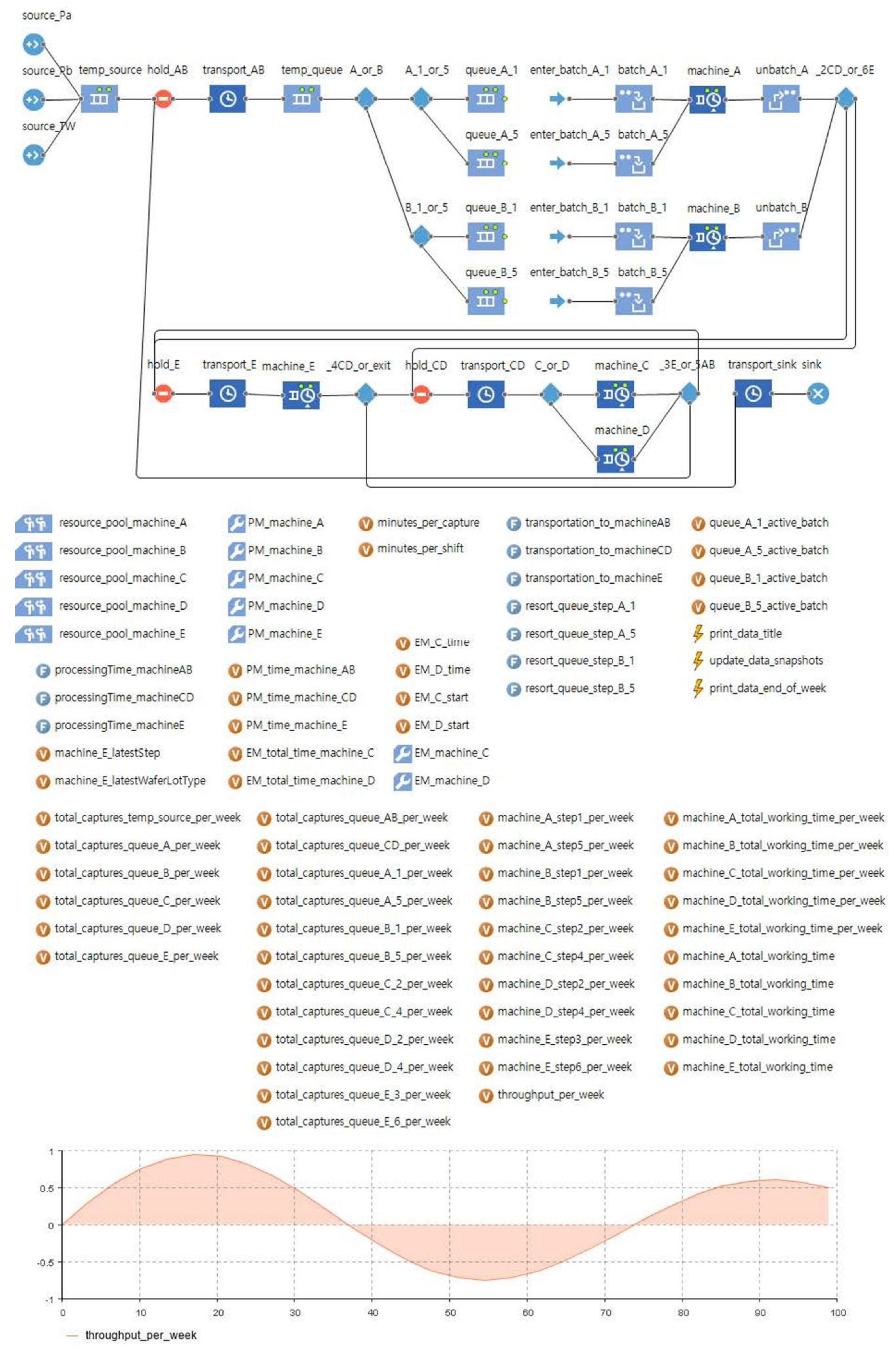
A simulation test bed using Anylogic 8.7.0 was developed based on the system above, as shown in Figure 2. The wafer lots were released every shift (one shift is 12 hours). Thus, the number of wafer lots to be released (per week) was distributed into 14 shifts (Table 2). The demand was released according to the generated schedule until the simulation was terminated. The recorded data were related to real-time production parameters, as listed in Table 3. The selection of production parameters was based on their importance according to previous studies: machine buffer capacity [30], machine utilization, and throughput [8]. The number of processing steps performed by each machine was added to consider the re-entrance characteristic in the studied semiconductor fab.
The throughput (data no. 43) was measured at the end of each week, in accordance with the target set in [26]. A set of data was measured from the start of a week until its end. Although there might be a slight effect from the decisions at the end of a shift on the earlier part of the next shift, we assumed that such an effect can be ignored. To compensate for this, we collected a large data set with various conditions at the start of each week.
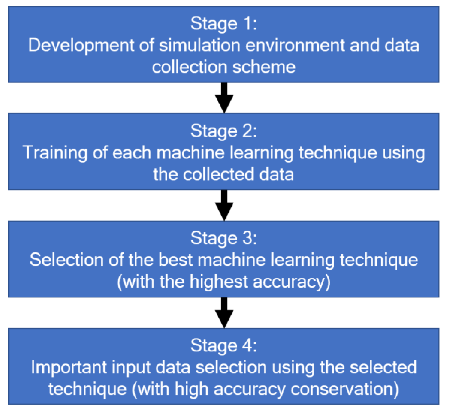
To assess the relationships between the data, analysis using machine learning techniques for classification (Table 4) was conducted. The flowchart of this study is presented in Figure 3. In stage 1, the simulation, using Anylogic, was developed based on the Intel minifab design and the data collection, as explained above. As a result of this stage, the recorded data was obtained and used for training each machine learning model listed in Table 4 (stage 2).
- Adaptive boosting (AB)The purpose of AB is to improve the performance of weak classifiers, such as the decision tree. The results of a previous classifier are inserted into the next one in a sequential training scheme. During this process, the mistakes of earlier classifiers are dealt with to improve the final prediction quality.
- Linear classifiers with stochastic gradient descent training (SGD)In SGD, estimation is conducted using linear models with stochastic gradient descent learning. The gradient of the loss is measured using each sample, and the model is updated with a certain decreased strength (learning rate).
- Neural network (multilayer perceptron) (NNMLP)NNMLP is a fully connected feed–forward network. The error propagation method is used for conducting the training.
- Gradient boosting (GB)GB is the improved version of the classification and regression tree (CART). Each new tree is generated in a serial order to correct the prediction error of the prior tree.
- Random forest (RF)RF uses decision trees for the classification task. The tree’s depth is increased by one, and this process is iterated for all nodes in the tree until a certain depth is reached.
- K-nearest neighbors (KNN)KNN predicts each data record in the test set by selecting the k nearest training set vectors. The classification is performed based on the majority of the votes.
- Classification and regression tree (CART)Training of the CART model includes tree generation through recursive binary splitting. Various split points are tested using a cost function, and the lowest cost-split is chosen to deal with the organized values.
- Naive bayes (gaussian) (NB)NB performs the classification based on the conditional probability of each categorical class variable. Such a maximum likelihood method is used for parameter estimation in various problem domains.
- Support vector machine (C-support vector) (SVM)SVM conducts the classification by generating N-dimensional hyperplanes that separate the data. Penalty factor C is considered to control the trade-off between allowing the existence of training errors and setting rigid margins.
The Python sklearn library [39] was applied in Visual Studio 2019 Community Platform to implement the machine learning techniques. When training each model, the following steps were conducted:
- Division of the collected data into training and testing data; the data before the division is shuffled, and the percentage of testing data is set equal to 20%.
- Testing accuracy of each model using k-fold cross-validation; the number of considered splits is ten. The training data are shuffled before the testing.
In stage 3, models with the best accuracy were selected. Until the current stage, all input data (data no. 1–42) were considered, but observing only some input data might be sufficient to predict the system’s throughput. Thus, in stage 4, the effect of reducing the input data to the throughput prediction accuracy changes was observed using the second step above. Given the complete input data, one input data was iteratively reduced, and the difference was observed. After checking all possible candidates in one iteration for reducing one data, the best accuracy was obtained. If the new prediction accuracy was the same or better than the current one, the input data combination was updated. In the end, the input data combination that produced the best accuracy was obtained. It was expected that identifying the important input data would help practitioners to focus their observations during the production period. The observation time was shortened, and more systemic insights could be obtained after analyzing the type of remaining input data. Finally, the testing data was fitted using the selected input data by calculating the precision, recall, f1-score, and support metrics.
4. Results
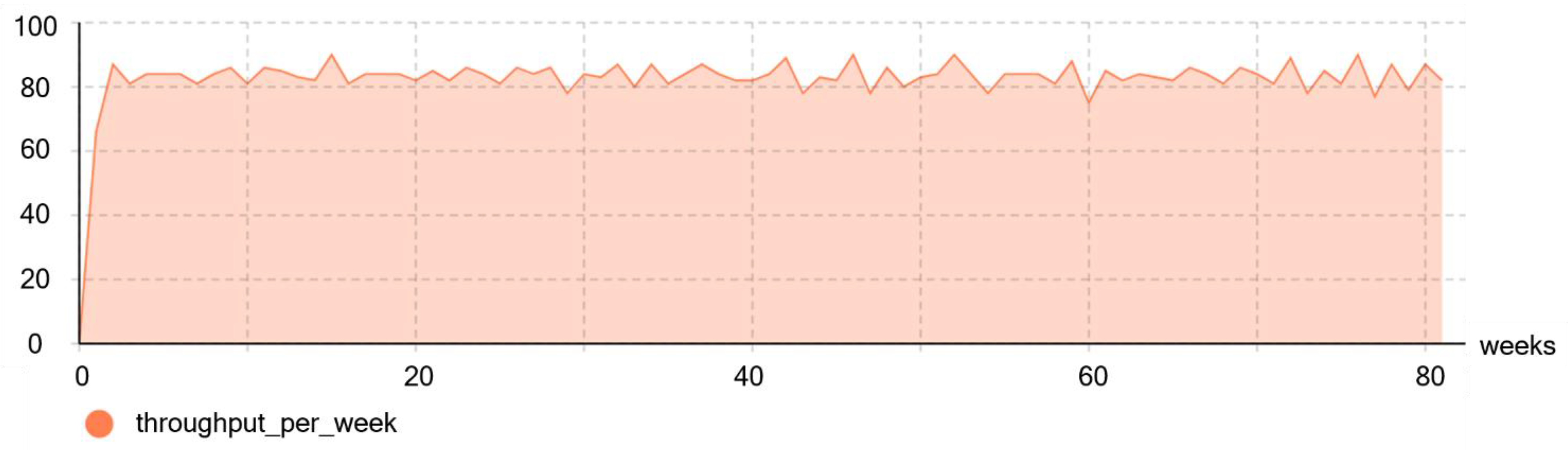
The simulation was run using random seed values from 0 to 30. The data was collected using each seed value after running the simulation for 325 weeks (on average). This observation period length was long enough, considering that, in practice, production control decisions should be made within shorter time periods (less than a year, ideally a few weeks or months) to ensure customers’ demand satisfaction is met. Given that the interval for capturing the simulation data was set to 1800 seconds and a shift equals 604,800 seconds, the number of data captures for each parameter in a week was 336 (that is, 604,800/1800). At the end of each week, each recorded parameter’s average value was obtained (accumulated value of each parameter in the week divided by the number of data captures per week). Data from 10,086 weeks were collected through the simulation after removing the records that were obtained during the warmup period. Each weekly data were considered to be in the warmup period if their value was less than the minimum throughput in the steady-state period; for example, the data in the first week of Figure 4. The data are available at https://github.com/ivanksinggih/Intel_minifab_Anylogic/tree/data (accessed on 7 February 2021).
The system’s throughput was between 73–95 wafer lots per week during the data collection period. The simulation had an average throughput (amount of lots per week) of 84 lots, which is same as the system’s initial design, so the developed simulation model was validated. It was expected that the system throughput would be at least equal to 84 wafer lots per week. Identifying appropriate system parameters to allow for more than 84 lots to be produced could allow additional demands to be satisfied. Thus, two classes were defined for the classification: (1) a “good” case, with throughput between 84–95 wafer lots per week, and (2) a “bad” case, with throughput between 73–83 lots per week. It was expected that using the selected model and input data set allow satisfying the target throughput and even having additional capacity to produce more lots.
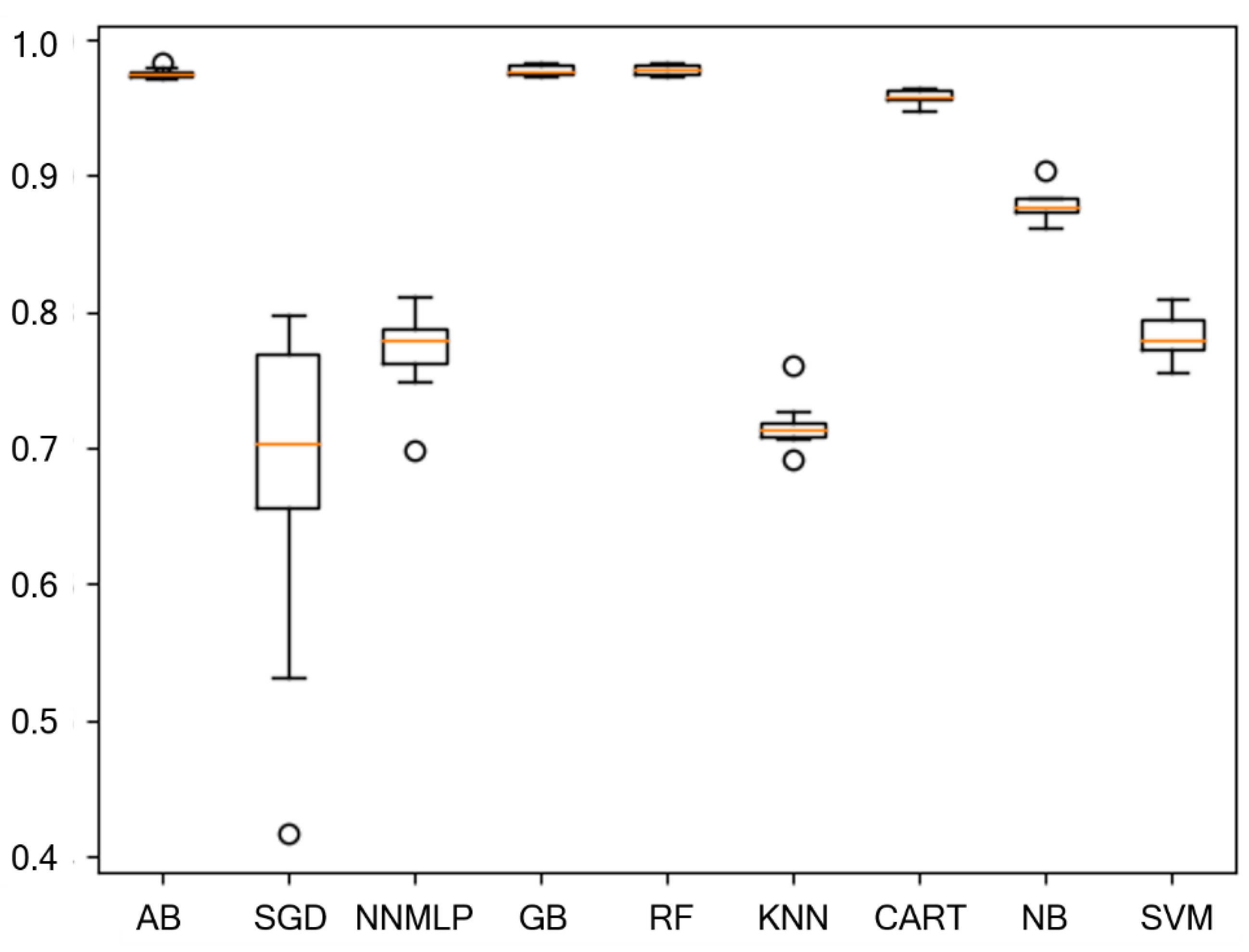
The result of accuracy testing for each machine learning technique is presented in Figure 5 (box plot) and Table 5. The methods with an accuracy of more than 95% are AB, GB, RF, and CART. As shown by the box plot, these four best methods also have a small deviation in their prediction results, which indicate that they were sufficiently reliable to produce good results in multiple runs. This fact is important considering that the selected prediction methods should be used to deal with new data obtained continuously from semiconductor fab that operates in high uncertainty (e.g., because of emergency maintenances). More observations were conducted to reduce the input data when using those four best methods. The final accuracies of those four best methods after reducing the input data are shown in Table 6. The AB, GB, and RF methods have slightly better accuracy than CART, and each of them considers different input data combinations when predicting the throughput.
Further analysis is required to identify whether a certain data group has more importance than others in the throughput prediction process. The input data are classified in two ways based on the following information: (1) data type and (2) machine-related data. The definition of each group and the input data inclusion into each group are presented in Table 7.
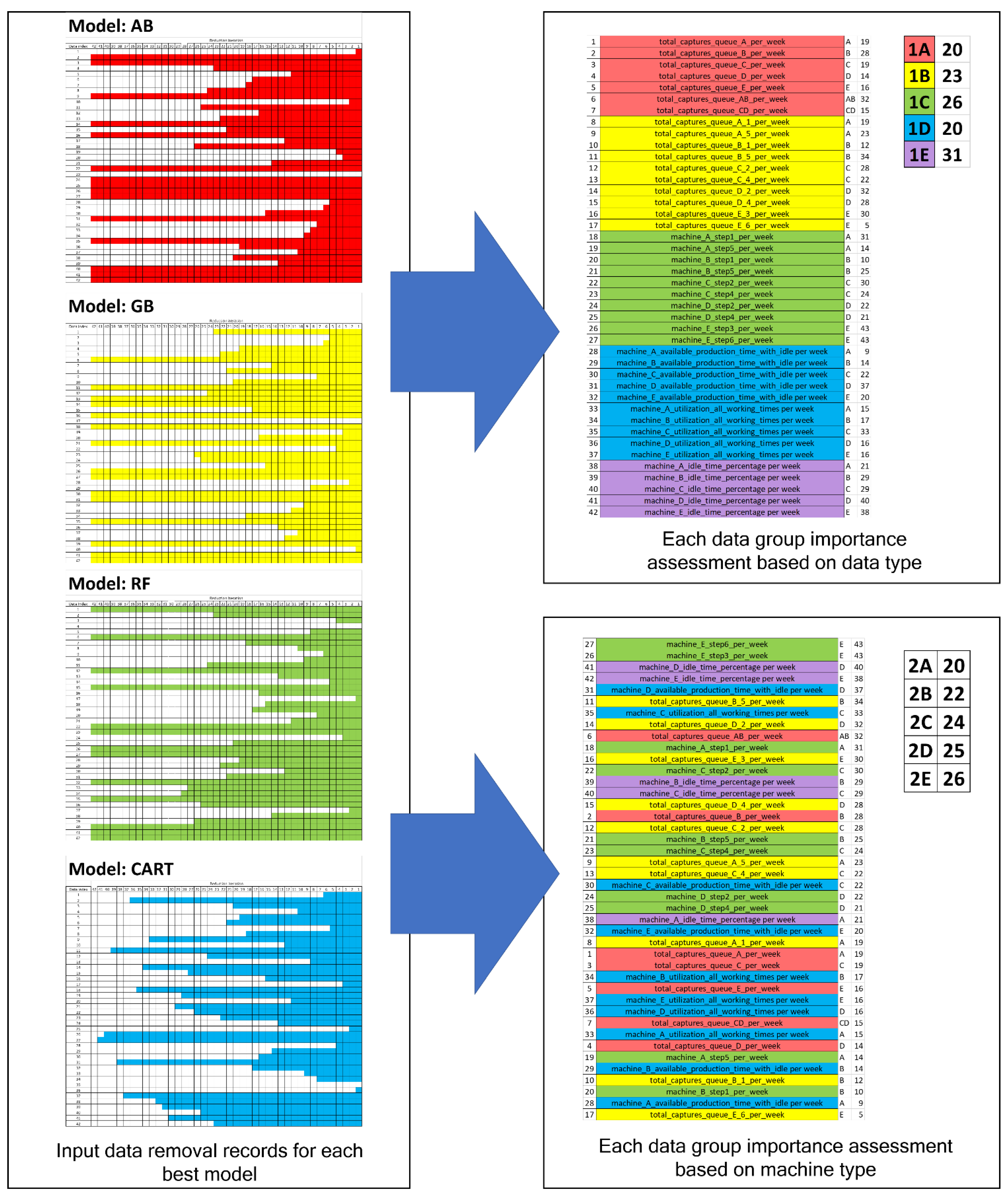
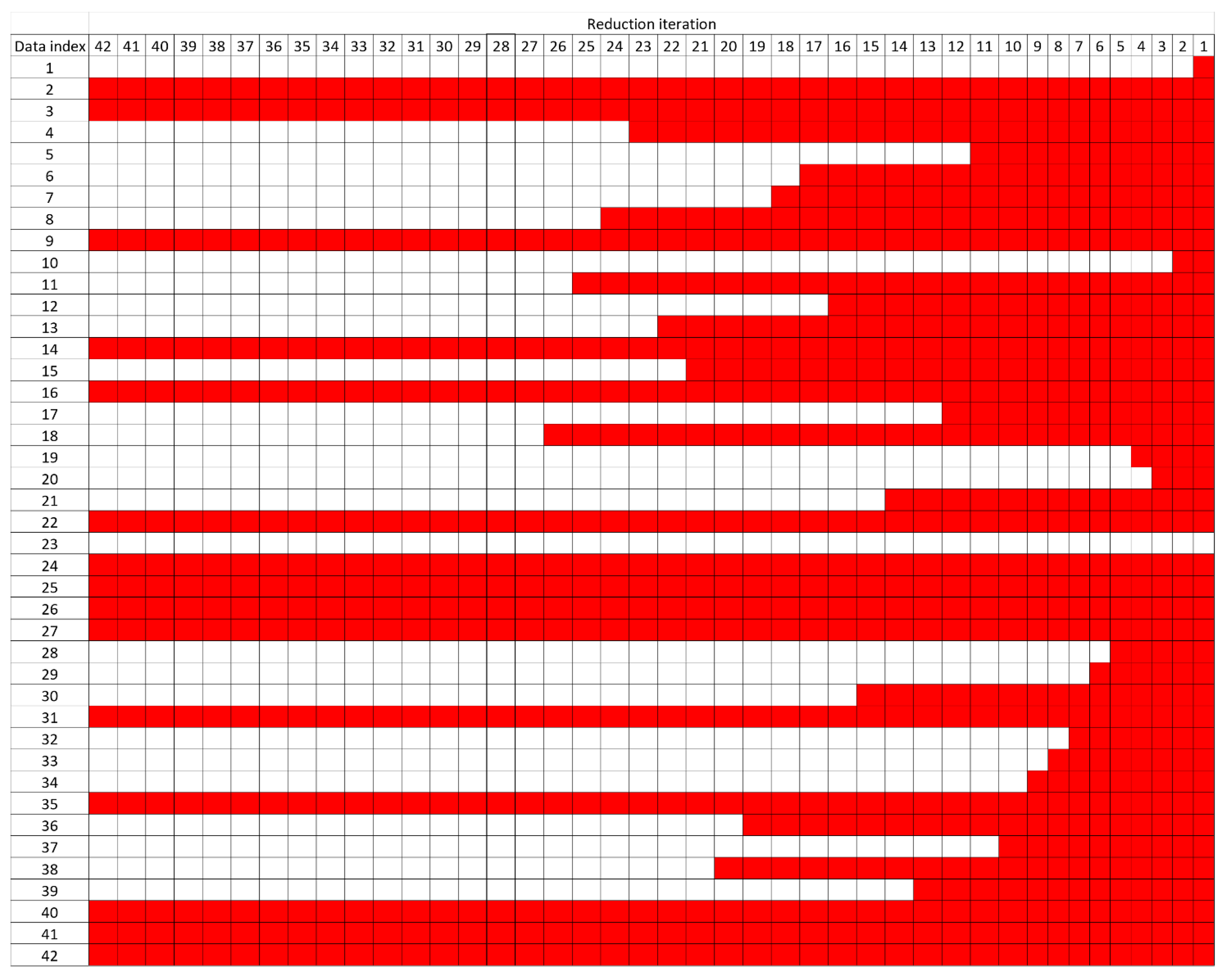
Each input data’s importance was further assessed by observing how long each of them was maintained when generating the final model, when using methods with the best accuracy (how long each of them remained within the iterations without being removed from the models). The analysis framework is presented in Figure 6. In the initial step (left part of Figure 6), the iteration index, the point at which each input data was removed, is recorded. An example of the AB model is presented in Figure 7. Based on Figure 7, input data 1 was removed in the first iteration (because its removal produces a new model with the least accuracy), input data 10 in the second iteration, input data 20 in the third iteration, and so on. The input data removal was stopped at iteration 28, because any input data removal at that iteration reduced the accuracy. When the iterations stopped, the final model’s remaining input data were marked as not removed until the end of the iterations (iteration 42).
In the next step of Figure 6 (right part of the figure), the obtained results from above are summarized based on the groups defined in Table 7. The values at the rightmost part of Figure 6 show the average iteration index, at which point the input data (in the group) were removed from the four best models. The data groups with larger average values contained input data that remained longer in the model. Input data in such groups had more effects on the predicted throughput.
When observed from the groupings based on the data types, the results show that the three most important data groups are the percentage of the machines’ total idle times (Group 1E), the number of processed wafer lots (with processing step consideration) (Group 1C), then the number of wafer lots waiting at each machine (with processing step consideration) (Group 1B). Input data in the machines’ total idle times group are important, because an appropriate idle time balance between the machines is required for processing the wafer lots and ensures smooth flows of the lots. Data in the number of processed wafer lots (with processing step consideration) group had more influence on the throughput prediction than the number of wafer lots waiting at the machines’ queues (input data in Group 1A and 1B). Thus, the wafer lot dispatching to the machines became an important decision to increase the system’s throughput. Regarding the number of waiting wafer lots data, input data in Group 1B were more important than that in Group 1A. This shows that ensuring an appropriate amount of wafer lots based on their processing steps was important to increase the throughput. Having wafer lots with a balanced amount of different processing steps ensured a more continuous flow of wafer lots compared with extreme cases, in which more wafer lots with earlier processing steps (steps 1, 2, 3) only, or with later processing steps (steps 4, 5, 6) only, were available in the machines’ queues. An unbalanced amount of wafer lots of each processing step could also disrupt the smooth flow of lots. An example of this was when more wafer lots with next processing steps 1, 3, and 5 were ready at the machines’ queues. In such a situation, the system produced fewer wafer lots with next processing steps 2, 4, and 6, which caused an insufficient supply of lots for executing processing steps 3 and 5.
When observed from the groupings based on the machine types, input data related to machine E (Group 2E) had slightly more importance than input data for other machines. The reason for this might be because machine E handles a higher workload (processing steps 3 and 6) than machines A and B (that together handle processing steps 1 and 5) and machines C and D (that handle processing steps 2 and 4). Having a good production plan and control for machine E will increase the throughput compared to focusing treatments on other machines.
The analysis above is derived from understanding how the system works. Future studies must conduct more detailed experiments, supported with statistical analysis, to identify the exact reasons the input data in some groups are more important than in others.
The four best machine learning techniques allowed good prediction of the real system. The results obtained using the testing data are presented in Table 8.
5. Conclusions
In this study, a simulation of a semiconductor fab based on the Intel minifab design was developed. The contributions of this study are as follows: (1) this is the first study to apply machine learning techniques to identify important real-time factors that influence throughput in the semiconductor fab; (2) this study developed a test bed in the Anylogic software environment based on the Intel minifab layout; and (3) this study proposed a data collection scheme for the production control mechanism.
To analyze production states that cause a high possibility of satisfying the required throughput, a data collection scheme was designed, and several machine learning techniques were compared. After training the model candidates, the four best models (adaptive boosting, gradient boosting, random forest, decision tree), with accuracies of more than 95%, were selected; and after reducing the input data, the models’ accuracy became 97.88%, 97.88%, 97.88%, and 97.82%, respectively. Further analysis showed that the machines’ total idle times and the number of wafer lots in the machines and their queues (with their processing step information), and data related to machine E, have more influence when predicting the throughput.
The following topics are recommended for future studies: (1) development and testing of actual production decisions (e.g., lot dispatching and rescheduling functions of the machines), considering the importance of the input data; and (2) the inclusion of the operators’ working time and limitations in the available material handling equipment. This study limited the observations to weekly data. It would be interesting for future studies to measure each shift’s input data (instead of each week’s). It is necessary to consider the sequence of values (or accumulated values) for the input data measured in consecutive shifts within each week. This is because decisions made in a shift have a great influence on the input data values in the next shift, considering the shorter length of a shift (compared with a week). Understanding the effect of each shift’s decisions will help practitioners achieve more accurate production control in each shift, while still reaching the required throughput at the end of each week.
Funding
This research received no external funding.
Institutional Review Board Statement
Not applicable.
Informed Consent Statement
Not applicable.
Data Availability Statement
Publicly available datasets were analyzed in this study. This data can be found here: https://github.com/ivanksinggih/Intel_minifab_Anylogic/tree/data (accessed on 7 February 2021).
Acknowledgments
The author would like to express his gratitude to Professor Bernardo Nugroho Yahya, who gave great advice during the paper revision process.
Conflicts of Interest
The author declares no conflict of interest.
References
- Hwang, I.; Jang, Y.J. Q(λ) learning-based dynamic route guidance algorithm for overhead hoist transport systems in semiconductor fabs. Int. J. Prod. Res. 2020, 58, 1199–1221. [Google Scholar] [CrossRef]
- Shahzad, M.A.; Gulzar, W.A. Industrie 4.0 readiness: Green computing in relation with key performance indicator for a manufacturing industry. Mob. Netw. Appl. 2020, 25, 1299–1306. [Google Scholar] [CrossRef]
- Lin, Z.; Matta, A.; Shanthikumar, J.G. Combining simulation experiments and analytical models with area-based accuracy for performance evaluation of manufacturing systems. IISE Trans. 2019, 51, 266–283. [Google Scholar] [CrossRef]
- Waschneck, B.; Reichstaller, A.; Belzner, L.; Altenmüller, T.; Bauernhansl, T.; Knapp, A.; Kyek, A. Deep reinforcement learning for semiconductor production scheduling. In Proceedings of the IEEE/SEMI Conference and Workshop on Advanced Semiconductor Manufacturing, New York, NY, USA, 30 April–3 May 2018; IEEE: Piscataway, NJ, USA, 2018; pp. 301–306. [Google Scholar] [CrossRef]
- Morariu, C.; Morariu, O.; Răileanu, S.; Borangiu, T. Machine learning for predictive scheduling and resource allocation in large scale manufacturing systems. Comput. Ind. 2020, 120, 103244. [Google Scholar] [CrossRef]
- Arinez, J.F.; Chang, Q.; Gao, R.X.; Xu, C.; Zhang, J. Artificial intelligence in advanced manufacturing: Current status and future outlook. ASME J. Manuf. Sci. Eng. 2020, 142, 11804. [Google Scholar] [CrossRef]
- Torres, D.; Pimentel, C.; Duarte, S. Shop floor management system in the context of smart manufacturing: A case study. Int. J. Lean Six Sigma 2020, 11, 837–862. [Google Scholar] [CrossRef]
- Alkan, B.; Bullock, S. Assessing operational complexity of manufacturing systems based on algorithmic complexity of key performance indicator time-series. J. Oper. Res. Soc. 2020, 1–15. [Google Scholar] [CrossRef]
- Gao, J. Performance evaluation of manufacturing collaborative logistics based on BP neural network and rough set. Neural. Comput. Appl. 2020. [Google Scholar] [CrossRef]
- Nath, S.; Sarkar, B. Performance evaluation of advanced manufacturing technologies: A De novo approach. Comput. Ind. Eng. 2017, 110, 364–378. [Google Scholar] [CrossRef]
- Saaty, T.L. The modern science of multicriteria decision making and its practical applications: The AHP/ANP approach. Oper. Res. 2013, 61, 1101–1118. [Google Scholar] [CrossRef]
- Zhong, R.Y. RFID data driven performance evaluation in production systems. Procedia CIRP. 2019, 81, 24–77. [Google Scholar] [CrossRef]
- Tin, T.C.; Chiew, K.L.; Phang, S.C.; Sze, S.N.; Tan, P.S. Incoming work-in-progress prediction in semiconductor fabrication foundry using long short-term memory. Comput. Intell. Neurosci. 2019, 8729367, 1–16. [Google Scholar] [CrossRef] [PubMed]
- Lingitz, L.; Gallina, V.; Ansari, F.; Gyulai, D.; Pfeiffer, A.; Sihn, W.; Monostori, L. Lead time prediction using machine learning algorithms: A case study by a semiconductor manufacturer. Procedia CIRP. 2018, 72, 1051–1056. [Google Scholar] [CrossRef]
- Lee, S.; Kim, H.J.; Kim, S.B. Dynamic dispatching system using a deep denoising autoencoder for semiconductor manufacturing. Appl. Soft Comput. 2020, 86, 105904. [Google Scholar] [CrossRef]
- Lee, S.; Kim, Y.; Kahng, H.; Lee, S.-K.; Chung, S.; Cheong, T.; Shin, K.; Park, J.; Kim, S.B. Intelligent traffic control for autonomous vehicle systems based on machine learning. Expert Syst. Appl. 2020, 144, 113074. [Google Scholar] [CrossRef]
- Hsu, C.-Y.; Chien, J.-C. Ensemble convolutional neural networks with weighted majority for wafer bin map pattern classification. J. Intell. Manuf. 2020. [Google Scholar] [CrossRef]
- Chien, J.-C.; Wu, M.-T.; Lee, J.-D. Inspection and classification of semiconductor wafer surface defects sing CNN deep learning networks. Appl. Sci. 2020, 10, 5340. [Google Scholar] [CrossRef]
- Fan, S.-K.S.; Hsu, C.-Y.; Tsai, D.-M.; He, F.; Cheng, C.-C. Data-driven approach for fault detection and diagnostic in semiconductor manufacturing. IEEE Trans. Autom. Sci. Eng. 2020, 17, 1925–1936. [Google Scholar] [CrossRef]
- Jiang, D.; Lin, W.; Raghavan, N. A novel framework for semiconductor manufacturing final test yield classification using machine learning techniques. IEEE Access. 2020, 8, 197885–197895. [Google Scholar] [CrossRef]
- Lee, D.-C.; Cho, S.-B. An agent-based system for abnormal flow detection in semiconductor production line. In Proceedings of the 17th International Conference on Control, Automation and Systems (ICCAS), Jeju, Korea, 18–21 October 2017; IEEE: Piscataway, NJ, USA, 2017; pp. 2015–2020. [Google Scholar] [CrossRef]
- Jang, S.-J.; Kim, J.-S.; Kim, T.-W.; Lee, H.-J.; Ko, S. A wafer map yield prediction based on machine learning for productivity enhancement. IEEE Trans. Semicond. Manuf. 2019, 32, 400–407. [Google Scholar] [CrossRef]
- Kim, J.-S.; Jang, S.-J.; Kim, T.-W.; Lee, H.-J.; Lee, J.-B. A productivity-oriented wafer map optimization using yield model based on machine learning. IEEE Trans. Semicond. Manuf. 2019, 32, 39–47. [Google Scholar] [CrossRef]
- Lauer, T.; Legner, S. Plan instability prediction by machine learning in master production planning. In Proceedings of the IEEE 15th International Conference on Automation Science and Engineering, Vancouver, BC, Canada, 22–26 August 2019; Curran Associates, Inc.: Red Hook, NY, USA, 2019; pp. 703–708. [Google Scholar] [CrossRef]
- Kang, Z.; Catal, C.; Tekinerdogan, B. Machine learning applications in production lines: A systematic literature review. Comput. Ind. Eng. 2020, 149, 106773. [Google Scholar] [CrossRef]
- Spier, J.; Kempf, K. Simulation of emergent behavior in manufacturing systems. In Proceedings of the SEMI Advanced Semiconductor Manufacturing Conference and Workshop, Cambridge, USA, 13–15 November 1995; IEEE: New York, NY, USA, 1995; pp. 90–94. [Google Scholar] [CrossRef]
- Dabbas, R.M.; Chen, H.-N.; Fowler, J.W.; Shunk, D. A combined dispatching criteria approach to scheduling semiconductor manufacturing systems. Comput. Ind. Eng. 2001, 39, 307–324. [Google Scholar] [CrossRef]
- Dabbas, R.M.; Fowler, J.W.; Rollier, D.A.; Mccarville, D. Multiple response optimization using mixture-designed experiments and desirability functions in semiconductor scheduling. Int. J. Prod. Res. 2003, 41, 939–961. [Google Scholar] [CrossRef]
- Li, Y.; Jiang, Z.; Jia, W. An integrated release and dispatch policy for semiconductor wafer fabrication. Int. J. Prod. Res. 2014, 52, 2275–2292. [Google Scholar] [CrossRef]
- Gu, X.; Guo, W.; Jin, X. Performance evaluation for manufacturing systems under control-limit maintenance policy. J. Manuf. Syst. 2020, 55, 221–232. [Google Scholar] [CrossRef]
- Liu, H.; Chen, C. Spatial air quality index prediction model based on decomposition, adaptive boosting, and three-stage feature selection: A case study in China. J. Clean. Prod. 2020, 265, 121777. [Google Scholar] [CrossRef]
- Ganesh, S.S.; Arulmozhicarman, P.; Tatavarti, R. Forecasting air quality index using an ensemble of artificial neural networks and regression models. J. Intell. Syst. 2017, 28, 893–903. [Google Scholar] [CrossRef]
- Zhang, Y.; Zhang, R.; Ma, Q.; Wang, Y.; Wang, Q.; Huang, Z.; Huang, L. A feature selection and multi-model fusion-based approach of predicting air quality. Isa Trans. 2019, 100, 210–220. [Google Scholar] [CrossRef]
- Liu, H.; Li, Q.; Yu, D.; Gu, Y. Air quality index and air pollutant concentration prediction based on machine learning algorithms. Appl. Sci. 2019, 9, 4069. [Google Scholar] [CrossRef] [Green Version]
- Kück, M.; Freitag, M. Forecasting of customer demands for production planning by local k-nearest neighbor models. Int. J Prod. Econ. 2021, 231, 107837. [Google Scholar] [CrossRef]
- Melgarejo, M.; Parra, C.; Oregón, N. Applying computational intelligence to the classification of pollution events. Int. Lat. Am. Trans. 2015, 13, 2071–2077. [Google Scholar] [CrossRef]
- Shi, G.-Y.; Liu, S. Model selection of c-support vector machines based on multi-threading genetic algorithm. Int. J. Wavelets. Multi. 2013, 11, 1350041. [Google Scholar] [CrossRef]
- Tama, B.A.; Lim, S. A comparative performance evaluation of classification algorithms for clinical decision support systems. Mathematics 2020, 8, 1814. [Google Scholar] [CrossRef]
- Pedregosa, F.; Varoquaux, G.; Gramfort, A.; Michel, V.; Thirion, B.; Grisel, O.; Blondel, M.; Prettenhofer, P.; Weiss, R.; Dubourg, V.; et al. Scikit-learn: Machine learning in Python. J. Mach. Learn. Res. 2011, 12, 2825–2830. [Google Scholar]
Figure 1.
The considered production control mechanism.

Figure 2.
Intel minifab test bed in the Anylogic software.

Figure 3.
Research flowchart of this study.

Figure 4.
Throughput changes during the warmup and data collection periods.

Figure 5.
Accuracy comparison of the considered machine learning techniques.

Figure 6.
Framework for analysis of each data group’s importance based on data and machine types.

Figure 7.
Iteration indices at which each input data is removed from Model AB.


Table 1.
Processing steps, machine eligibilities, and time information for the Intel minifab system.
Table 1.
Processing steps, machine eligibilities, and time information for the Intel minifab system.
| Processing Steps | Machine A & B | Machine C & D | Machine E | ||||||
|---|---|---|---|---|---|---|---|---|---|
| L | P | U | L | P | U | L | P | U | |
| step 1 | 1200 | 13,500 | 2400 | ||||||
| step 2 | 900 | 1800 | 900 | ||||||
| step 3 | 600 | 3300 | 600 | ||||||
| step 4 | 900 | 3000 | 900 | ||||||
| step 5 | 1200 | 15,300 | 2400 | ||||||
| step 6 | 600 | 600 | 600 | ||||||
L = loading time, P = processing time, U = unloading time (in seconds).
Table 2.
Wafer lot release schedule per shift (for one week).
| Number of Released Wafer Lots | |||
|---|---|---|---|
| Shift | Pa | Pb | TW |
| shift 1 | 3 | 2 | 1 |
| shift 2 | 4 | 2 | 0 |
| shift 3 | 4 | 2 | 0 |
| shift 4 | 3 | 3 | 0 |
| shift 5 | 4 | 2 | 0 |
| shift 6 | 4 | 2 | 0 |
| shift 7 | 3 | 2 | 1 |
| shift 8 | 4 | 2 | 0 |
| shift 9 | 4 | 2 | 0 |
| shift 10 | 3 | 3 | 0 |
| shift 11 | 4 | 2 | 0 |
| shift 12 | 4 | 2 | 0 |
| shift 13 | 3 | 2 | 1 |
| shift 14 | 4 | 2 | 0 |
| total | 51 | 30 | 3 |
Table 3.
Collected data in the simulation.
| Data No. | Data Name | Description |
|---|---|---|
| 1 | total_captures_queue_A_per_week | number of wafer lots waiting at machine A’s buffer in one week |
| 2 | total_captures_queue_B_per_week | number of wafer lots waiting at machine B’s buffer in one week |
| 3 | total_captures_queue_C_per_week | number of wafer lots waiting at machine C’s buffer in one week |
| 4 | total_captures_queue_D_per_week | number of wafer lots waiting at machine D’s buffer in one week |
| 5 | total_captures_queue_E_per_week | number of wafer lots waiting at machine E’s buffer in one week |
| 6 | total_captures_queue_AB_per_week | number of wafer lots waiting at machine A’s and machine B’s buffers in one week |
| 7 | total_captures_queue_CD_per_week | number of wafer lots waiting at machine C’s and machine D’s buffers in one week |
| 8 | total_captures_queue_A_1_per_week | number of wafer lots with processing step 1 waiting at machine A’s buffer in one week |
| 9 | total_captures_queue_A_5_per_week | number of wafer lots with processing step 5 waiting at machine A’s buffer in one week |
| 10 | total_captures_queue_B_1_per_week | number of wafer lots with processing step 1 waiting at machine B’s buffer in one week |
| 11 | total_captures_queue_B_5_per_week | number of wafer lots with processing step 5 waiting at machine B’s buffer in one week |
| 12 | total_captures_queue_C_2_per_week | number of wafer lots with processing step 2 waiting at machine C’s buffer in one week |
| 13 | total_captures_queue_C_4_per_week | number of wafer lots with processing step 4 waiting at machine C’s buffer in one week |
| 14 | total_captures_queue_D_2_per_week | number of wafer lots with processing step 2 waiting at machine D’s buffer in one week |
| 15 | total_captures_queue_D_4_per_week | number of wafer lots with processing step 4 waiting at machine D’s buffer in one week |
| 16 | total_captures_queue_E_3_per_week | number of wafer lots with processing step 3 waiting at machine E’s buffer in one week |
| 17 | total_captures_queue_E_6_per_week | number of wafer lots with processing step 6 waiting at machine E’s buffer in one week |
| 18 | machine_A_step1_per_week | number of wafer lots with step 1 processed at machine A in one week |
| 19 | machine_A_step5_per_week | number of wafer lots with step 5 processed at machine A in one week |
| 20 | machine_B_step1_per_week | number of wafer lots with step 1 processed at machine B in one week |
| 21 | machine_B_step5_per_week | number of wafer lots with step 5 processed at machine B in one week |
| 22 | machine_C_step2_per_week | number of wafer lots with step 2 processed at machine C in one week |
| 23 | machine_C_step4_per_week | number of wafer lots with step 4 processed at machine C in one week |
| 24 | machine_D_step2_per_week | number of wafer lots with step 2 processed at machine D in one week |
| 25 | machine_D_step4_per_week | number of wafer lots with step 4 processed at machine D in one week |
| 26 | machine_E_step3_per_week | number of wafer lots with step 3 processed at machine E in one week |
| 27 | machine_E_step6_per_week | number of wafer lots with step 6 processed at machine E in one week |
| 28 | machine_A_available_production_ time_with_idle_per_week | percentage of machine A’s available production time after excluding the preventive and emergency maintenances in one week |
| 29 | machine_B_available_production_ time_with_idle_per_week | percentage of machine B’s available production time after excluding the preventive and emergency maintenances in one week |
| 30 | machine_C_available_production_ time_with_idle_per_week | percentage of machine C’s available production time after excluding the preventive and emergency maintenances in one week |
| 31 | machine_D_available_production_ time_with_idle_per_week | percentage of machine D’s available production time after excluding the preventive and emergency maintenances in one week |
| 32 | machine_E_available_production_ time_with_idle_per_week | percentage of machine E’s available production time after excluding the preventive and emergency maintenances in one week |
| 33 | machine_A_utilization_ all_working_times_per_week | percentage of machine A’s actual production time after excluding the preventive maintenance, emergency maintenance, and idle times in one week |
| 34 | machine_B_utilization_ all_working_times_per_week | percentage of machine B’s actual production time after excluding the preventive maintenance, emergency maintenance, and idle times in one week |
| 35 | machine_C_utilization_ all_working_times_per_week | percentage of machine C’s actual production time after excluding the preventive maintenance, emergency maintenance, and idle times in one week |
| 36 | machine_D_utilization_ all_working_times_per_week | percentage of machine D’s actual production time after excluding the preventive maintenance, emergency maintenance, and idle times in one week |
| 37 | machine_E_utilization_ all_working_times_per_week | percentage of machine E’s actual production time after excluding the preventive maintenance, emergency maintenance, and idle times in one week |
| 38 | machine_A_idle_time_ percentage_per week | percentage of machine A’s total idle time in one week |
| 39 | machine_B_idle_time_ percentage_per week | percentage of machine B’s total idle time in one week |
| 40 | machine_C_idle_time_ percentage_per week | percentage of machine C’s total idle time in one week |
| 41 | machine_D_idle_time_ percentage_per week | percentage of machine D’s total idle time in one week |
| 42 | machine_E_idle_time_ percentage_per week | percentage of machine E’s total idle time in one week |
| 43 | throughput_per_week | number of wafer lot finished in one week |
Table 4.
Machine learning techniques applied in this study.
| Machine Learning Technique | Reference |
|---|---|
| adaptive boosting (AB) | [31] |
| linear classifiers with stochastic gradient descent training (SGD) | [32] |
| neural network (multilayer perceptron 1) (NNMLP) | [32] |
| gradient boosting (GB) | [33] |
| random forest (RF) | [34] |
| k-nearest neighbors (KNN) | [35] |
| classification and regression tree (CART) | [33] |
| naive bayes (gaussian 1) (NB) | [36] |
| support vector machine (C-support vector 1) (SVM) | [37] |
1 Specific methods that are considered in this study.
Table 5.
Obtained accuracy of each machine learning technique.
| Machine Learning Technique | Accuracy |
|---|---|
| adaptive boosting (AB) | 97.57% 1 |
| linear classifiers with stochastic gradient descent training (SGD) | 67.96% |
| neural network (multilayer perceptron) (NNMLP) | 77.27% |
| gradient boosting (GB) | 97.78% 1 |
| random forest (RF) | 97.83% 1 |
| k-nearest neighbors (KNN) | 71.70% |
| decision tree (CART) | 95.80% 1 |
| naive bayes (gaussian) (NB) | 87.85% |
| support vector machine (C-support vector) (SVM) | 78.31% |
1 More than 95% accuracy.
Table 6.
Accuracy of each machine learning technique after reduction of input data.
| Best Model | Input Data Combination (with Indices in Table 3) | Accuracy (with Selected Input Parameters) |
|---|---|---|
| AB | 2–3, 9, 14, 16, 18, 22, 24–27, 31, 35, 40–42 | 97.88% 1 |
| GB | 6, 11, 13–14, 16, 18, 21, 26–27, 30–31, 35, 39, 41–42 | 97.88% 1 |
| RF | 1, 6, 12, 15, 22–23, 26–27, 32, 35, 41–42 | 97.88% 1 |
| CART | 27 | 97.82% |
1 Combination of input data with the best accuracy among the best models.
Table 7.
Input data groups based on (1) data type and (2) machine-related data information.
| Grouping Rule | Groups and Definitions | Included Input Data |
|---|---|---|
| (1) data type | (group 1A) number of wafer lots waiting at each machine (without processing step consideration) | 1–7 |
| (group 1B) number of wafer lots waiting at each machine (with processing step consideration) | 8–17 | |
| (group 1C) number of processed wafer lots (with processing step consideration) | 18–27 | |
| (group 1D) percentages of available machines’ production times after excluding maintenance times | 28–37 | |
| (group 1E) percentage of machines’ total idle times | 38–42 | |
| (2) machine | (group 2A) machine A-related input data | 1,6,8–9,18–19,28,33,38 |
| (group 2B) machine B-related input data | 2,6,10–11,20–21,29,34,39 | |
| (group 2C) machine C-related input data | 3,7,12–13,22–23,30,35,40 | |
| (group 2D) machine D-related input data | 4,7,14–15,24–25,31,36,41 | |
| (group 2E) machine E-related input data | 5,16–17,26–27,32,37,42 |
Table 8.
Precision, recall, f1-score, and support values obtained using the testing data.
| Best Model | Data Class | Evaluation Metrics | Number of Correctly Classified Data | |||
|---|---|---|---|---|---|---|
| Precision | Recall | F1-score | Support | |||
| AB | good | 0.98 | 0.95 | 0.96 | 729 | 691 |
| bad | 0.97 | 0.99 | 0.98 | 1289 | 1275 | |
| GB | good | 0.98 | 0.96 | 0.97 | 729 | 699 |
| bad | 0.98 | 0.99 | 0.98 | 1289 | 1272 | |
| RF | good | 0.98 | 0.96 | 0.97 | 729 | 699 |
| bad | 0.98 | 0.99 | 0.98 | 1289 | 1272 | |
| CART | good | 0.98 | 0.96 | 0.97 | 729 | 699 |
| bad | 0.98 | 0.99 | 0.98 | 1289 | 1272 | |
Publisher’s Note: MDPI stays neutral with regard to jurisdictional claims in published maps and institutional affiliations. |
© 2021 by the author. Licensee MDPI, Basel, Switzerland. This article is an open access article distributed under the terms and conditions of the Creative Commons Attribution (CC BY) license (http://creativecommons.org/licenses/by/4.0/).
Share and Cite
MDPI and ACS Style
Singgih, I.K. Production Flow Analysis in a Semiconductor Fab Using Machine Learning Techniques. Processes 2021, 9, 407. https://0-doi-org.brum.beds.ac.uk/10.3390/pr9030407
AMA Style
Singgih IK. Production Flow Analysis in a Semiconductor Fab Using Machine Learning Techniques. Processes. 2021; 9(3):407. https://0-doi-org.brum.beds.ac.uk/10.3390/pr9030407
Chicago/Turabian StyleSinggih, Ivan Kristianto. 2021. "Production Flow Analysis in a Semiconductor Fab Using Machine Learning Techniques" Processes 9, no. 3: 407. https://0-doi-org.brum.beds.ac.uk/10.3390/pr9030407
Note that from the first issue of 2016, this journal uses article numbers instead of page numbers. See further details here.