Noises Cutting and Natural Neighbors Spectral Clustering Based on Coupling P System

Abstract

Clustering analysis, a key step for many data mining problems, can be applied to various fields. However, no matter what kind of clustering method, noise points have always been an important factor affecting the clustering effect. In addition, in spectral clustering, the construction of affinity matrix affects the formation of new samples, which in turn affects the final clustering results. Therefore, this study proposes a noise cutting and natural neighbors spectral clustering method based on coupling P system (NCNNSC-CP) to solve the above problems. The whole algorithm process is carried out in the coupled P system. We propose a natural neighbors searching method without parameters, which can quickly determine the natural neighbors and natural characteristic value of data points. Then, based on it, the critical density and reverse density are obtained, and noise identification and cutting are performed. The affinity matrix constructed using core natural neighbors greatly improve the similarity between data points. Experimental results on nine synthetic data sets and six UCI datasets demonstrate that the proposed algorithm is better than other comparison algorithms.

1. Introduction

With the rapid development of information technology, many fields have accumulated massive data. How to mine significant information and useful knowledge is a huge challenge. Clustering analysis, a key step for many data mining problems, can be applied to a variety of data types. The purpose of clustering is to divide a set of unlabeled data into different clusters based on the similarity between the data [1]. Therefore, the data with the most similar characteristics will be in the same cluster, while the data with the most dissimilar characteristics will be in different clusters [2]. Predecessors have proposed many clustering methods, such as partitioning methods [3], hierarchical methods [4], density methods [5,6], grid methods [7], and prototype-based methods [8]. Over the past few decades, clustering analysis has been effectively applied in image segmentation [9], text clustering [10], community division [11], pattern recognition [12], etc.

In recent years, spectral clustering, an effective clustering algorithm based on graph theory, has attracted the attention in academia because of its high performance and simple implementation [13]. Spectral clustering can identify samples with arbitrary shapes while converging to the global optimal solution. Its main idea is to treat all data as nodes in space, and these nodes can be connected by edges. The weight of the edge between two nodes is determined by their distance. The distance that is closer shows that the higher the similarity, so it has higher weight, and vice versa. Then, according to the graph partition method, the graph is divided into several disconnected sub-graphs. The weight sum of edges between different sub-graphs is as small as possible, and the weight sum of edges within a sub-graph is as high as possible. The set of nodes contained in the sub-graph is the final clustering result [14]. Spectral clustering can be understood as mapping data in high-dimensional space to low-dimensional, and then clustering in low-dimensional space using other clustering algorithms (such as K-means).

In the spectral clustering algorithm, an important problem is constructing the affinity matrix. Yessica and Miin-Shen [2] merged the power parameter into the Gaussian kernel similarity function for the construction of affinity matrix. This power parameter can separate the points actually located on different clusters, but the distance is small. Then, it uses the maximum of all the minimum distances between the data nodes to obtain better clustering results. The maximum value between the estimated power parameter and the minimum distance can effectively improve the effect of spectral clustering. Huang et al. [15] proposed two novel algorithms—ultra-scalable spectral clustering (U-SPEC) and ultra-scalable ensemble clustering (U-SENC)—based on ultra-large-scale data under limited resources. In U-SPEC, first, in order to construct a sparse affinity sub-matrix, a hybrid representative selection strategy and a fast approximation method of k-nearest representative are proposed. Then, it interprets the sparse sub-matrix as a bipartite graph. Finally, using transfer cutting partitions the graph effectively and achieves the clustering result. In U-SENC, by integrating multiple U-SPEC clusters, a new bipartite graph is constructed between the nodes and the base clusters, and then the effective division is performed to obtain consistent clustering results. Bian et al. [16] combined spectral clustering structure and data fuzzy similarity matrix learning method (FSCM) to enhance the clustering performance. FCSM adopts the dual-index fuzzy c-means clustering algorithm to determine the fuzzy similarity between any pair of data points. Meanwhile, it generates the fuzzy similarity matrix of the data by adaptively assigning the fuzzy neighborhood of the data points. In this way, the spectral clustering structure of the data is found and the clustering stability of the FSCM algorithm is ensured. Lin and Guo [17] put forward a new affinity matrix generation method based on the principle of neighbor relationship propagation and gave a neighbor relationship propagation algorithm. The generated affinity matrix can effectively promote the similarity of point pairs in the same cluster and can better identify the structure of the data. Aiming at the similarity measurement of complex data, Xiucai and Tetsuya [18] proposed a novel spectral clustering method, which is based on the similarity measurement of data points in the kernel space adaptive neighborhood. In the kernel space, adaptive and optimal neighbors are assigned to each data point according to the local structure, and the sparse matrix is learned as a similarity matrix for spectral clustering. Wu et al. [19] present a scalable spectral clustering method based on Random Binning features (RB), which can accelerate the construction and feature decomposition of similar graphs at the same time. In detail, it constructs the inner product implicit approximation graph similarity (kernel) matrix of a large sparse feature matrix through RB.

Membrane computing [20] (also known as P system) is a system with the characteristics of distributed parallel computing proposed by Professor Păun. Its purpose is to learn from and simulate the way cells, tissues, organs, or other biological structures process chemical substances and establish a distributed parallel computing model with outstanding computing performance [21]. P system is a novel branch of natural computing, which provides an abundant computing framework for bimolecular computing. P system has been proved to have the calculation ability equivalent to Turing machine, and can effectively solve the difficult problem of calculation [22]. Nowadays, the P system is mainly divided into cell-like P system, tissue-like P system, and neural-like P system [23]. In recent years, the research content of the P system mainly includes theoretical research and application research. In terms of theoretical research, some new variants of the P system have been proposed to solve the problem, which can improve the computing power with the min cells or spikes [24,25]. For application research, the P system can solve practical problems [26] and can be used to implement clustering processes [27,28].

Although the above algorithm can achieve better clustering performance, to a certain extent, noise points also have a great influence on the clustering effect. At the same time, the determination of the parameters of natural neighbors is also an important issue when constructing the affinity matrix. To address above problems and based on the above analysis, we propose a spectral clustering method with noises cutting and natural neighbors based on the coupling P system (NCNNSC-CP) and verify clustering performance. The main contributions of this paper are as follows:

(1) A new coupling P system is proposed, which integrates natural neighbors and spectral clustering into the coupling membrane system to perform clustering tasks.

(2) Aiming at the noise points in the data set, we utilize the characteristics of the natural neighbors to identify and cut the noise points.

(3) In the stage of spectral clustering, we propose a search of natural neighbors without parameters, which can quickly determine the natural eigenvalues, thereby further constructing an affinity matrix with high similarity within the cluster.

(4) Nine classical synthetic data sets and six UCI data sets are used to simulate and verify the clustering performances of NCNNSC-CP.

The rest of the paper is organized as follows. Section 2 introduces the related concepts of P system and natural neighbors, and the basic algorithm of spectral clustering. In Section 3, a spectral clustering method with noises cutting and natural neighbors based on the coupling P system is proposed. Section 4 shows the performance of the algorithm through experimental analysis. Conclusions and future research work are given in Section 5.

2. Related Work

2.1. Spectral Clustering

The spectral clustering algorithm is based on graph theory. Compared with traditional clustering algorithms, it can cluster data points with arbitrary shapes and converge to the global optimal solution efficiently. First, it constructs an undirected weighted graph $G(V,E)$ based on similarity. Each $v_i$ of the graphs corresponds to a data point, and the weight $w_{ij}$ is the similarity of the edges formed by the data points. Generally, there are three ways to construct an affinity matrix:

(1) $\epsilon$-neighborhood graph. Set the distance threshold $\epsilon$, Euclidean distance $s_{ij}=\left|\right|x_i-x_j|{|}_2^2$. $w_{ij}=\epsilon$, if $s_{ij}<\epsilon$; otherwise, $w_{ij}=0$.

(2) K-nearest neighbor graph. Using the KNN algorithm obtains the k neighbors of each data point, only when $x_j$ is one of the k neighbors of $x_i$$w_{ij}>0$, and $w_{ij}=\exp (-\frac{\left|\right|x_i-x_j|{|}_2^2}{2{\sigma }^2})$.

(3) Fully connected graph. In general spectral clustering, it is the most commonly used method of constructing affinity matrix. Different kernel functions can be selected to define the weight between edges. When using Gaussian kernel function, the similarity matrix and the affinity matrix are the same, $w_{ij}=s_{ij}=\exp (-\frac{\left|\right|x_i-x_j|{|}_2^2}{2{\sigma }^2})$.

Then, according to the affinity matrix, we construct the degree matrix D. For any point $x_i$ in the graph, its degree $d_i$ is defined as the sum of the weights of all edges connected to it $d_i={\displaystyle {\sum }_{j=1}^n{w}_{ij}}.$ The most important process in spectral clustering is the construction of Laplacian matrix L:

(1) The denormalized Laplacian matrix $L=D-W.$

(2) Normalized Laplacian matrix based on Random Walk $L=I-D^{-1}W{D}^{-1}.$

(3) Symmetric normalized Laplacian matrix $L=I-D^{-1/2}W{D}^{-1/2}.$

Next, the eigenvector $u_1,u_2,\cdots u_k$ corresponding to the first k eigenvalues of the L can be calculated and set: $U=\{u_1,u_2,\cdots u_k\},U\in R^{n\ast k}$. In addition, U is normalized by row to generate $Y=\{y_1,y_2,\cdots y_n\}$, and each row of Y represents a sample. At last, the clustering algorithm (such as k-means) is applied to cluster the new samples into clusters $C_1,C_2,\cdots C_k$.

The basic spectral clustering algorithm (NJW) [29] is shown in Algorithm 1.

Algorithm 1 Spectral clustering (NJW)

Input: The dataset D

Output: C (the clustering results)

1: Construct the affinity matrix W.

2: Degree matrix D, $d_i={\displaystyle {\sum }_{j=1}^n{w}_{ij}}.$

3: Laplacian matrix $L=I-D^{-1/2}W{D}^{-1/2}.$

4: Construct the feature matrix $U=\{u_1,u_2,\cdots u_k\},U\in R^{n\ast k}$

5: Form the matrix Y from U, $Y_{ij}=U_{ij}/{({\displaystyle {\sum }_j{U}_{ij}^2})}^{1/2}$

6: C = K-means(Y)

2.2. Natural Neighbors

Zhu [30] systematically expounded the concept of natural neighbors through induction and summary based on previous studies, which is a reflection of the friendship between people in human society. Compared with the traditional nearest neighbor method, the natural neighbor method is scale-free. The relevant definitions of natural neighbors are as follows.

Definition 1:

(The Natural Neighbor Stable Structure).The natural neighbor stable structure is, generally speaking, that A is a Natural Neighbor of B if A regards B as a neighbor and B regards A as a neighbor at the same time.

$$(\forall x_i)(\exists x_j)(k\in N)\wedge (i\ne j)\to (x_i\in N{N}_k(x_j))\wedge (x_j\in N{N}_k(x_i))$$

(1)

where NNk(x_i) is the kth nearest neighbor of point x_i.

Definition 2:

(k-Nearest Neighbors).Given a data set D, for any point$x_i$, its k nearest neighbors refer to a set of points in D with$d(x_i,x)\le d(x_i,\mathrm{o})$, which is

$$N{N}_k(x_i)=\{x_j\in D|d(x_i,x_j)\le d(x_i,kn)\}$$

(2)

where$d(x_i,kn)$is the distance of the kth nearest neighbor of$x_i$.

Definition 3:

(Reverse Neighbors).The reverse neighbor of$x_i$is considered to be a set of data points x in D that take$x_i$as its k nearest neighbor, which is

$$RNN(x_i)=\{x\in D|x_i\in N{N}_k(x)\}$$

(3)

Definition 4:

(The Natural Characteristic Value Sup [31]).Sup is the search range in the natural neighbor method.

$$Sup=\min \{k|{\displaystyle \sum _{i=1}^{n}f(N{b}_k(x_i))}=0\hspace{0.17em}or\hspace{0.17em}{\displaystyle \sum _{i=1}^{n}f(N{b}_k(x_i))}={\displaystyle \sum _{i=1}^{n}f(N{b}_{k-1}(x_i))}\}$$

(4)

where the initial value of k is 1, and$N{b}_k(x_i)$is the number of reverse neighbors of$x_i$in the kth iteration. In addition,$f(x)=\{\begin{array}{l}0,\hspace{0.17em}\hspace{0.17em}otherwise\\ 1,\hspace{0.17em}\hspace{0.17em}if\hspace{0.17em}x==0\end{array}.$

Definition 5:

(The Natural Neighbors).For each object x in dataset D, its natural neighbors are k nearest neighbors, denoted as NaN (x).

2.3. Cell-Like and Tissue-Like P System

2.3.1. Cell-Like P System

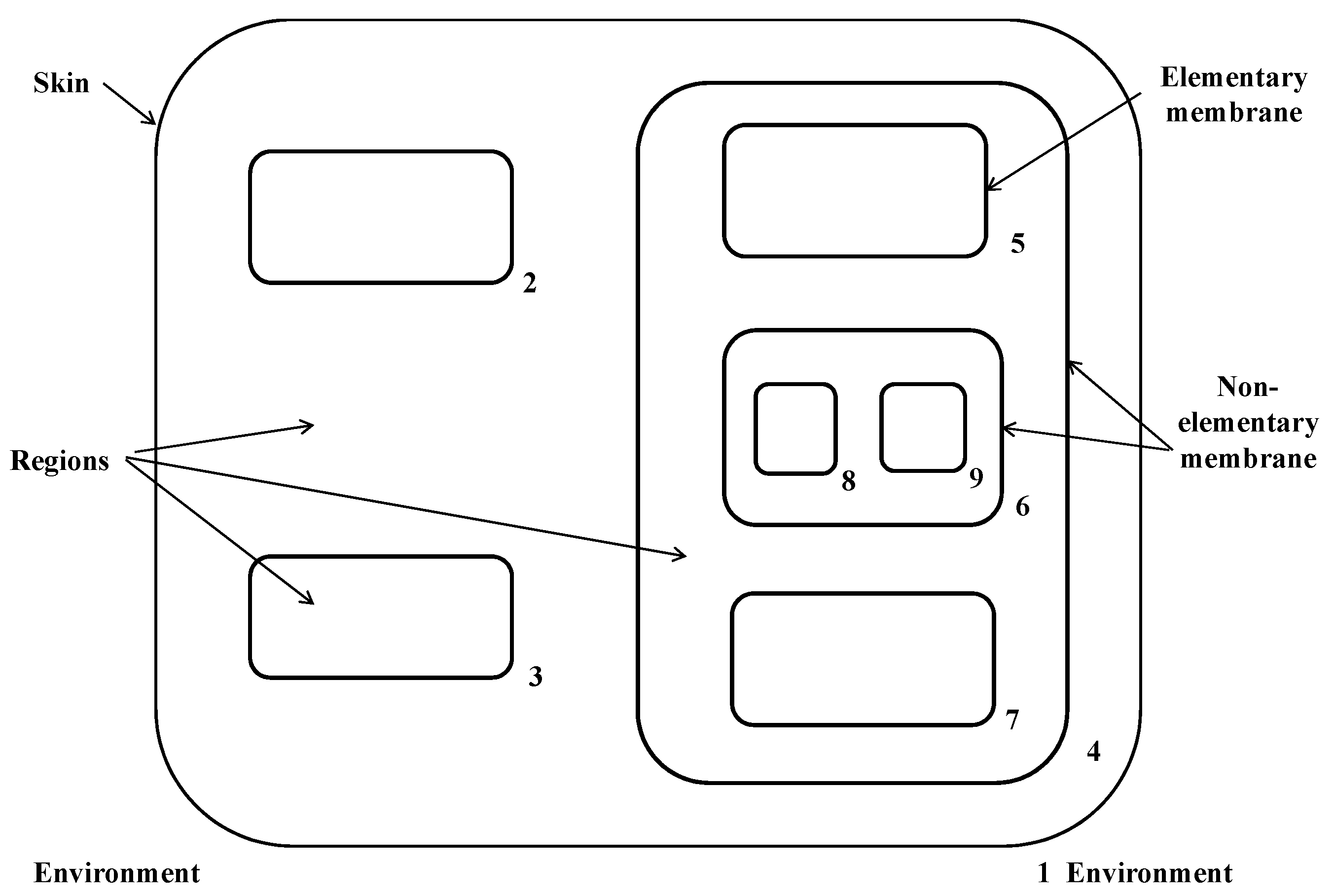
The cell-like P system is the first proposed P system, and its membrane structure is shown in Figure 1. The outermost membrane 1 is the skin membrane. The skin membrane separates the entire P system from the external environment. If a membrane does not contain a submembrane inside, the membrane is a basic membrane (such as membrane s2, 3, 5, 8, 9, and 7). Otherwise, it is called a non-basic membrane (such as membranes 1, 4, and 6).

The formal definition of the cell-like P system is

$$\prod =(O,H,\mu ,{\omega }_1,\cdots ,{\omega }_m,R,i_0)$$

where

• O is the alphabet, where the elements represent objects;
• H is a collection of membrane labels;
• $\mu$ represents the membrane structure;
• ${\omega }_i(1\le i\le m)$ refers to the multiple set of objects contained in region $i$ in the membrane structure;
• R contains all the rules;
• $i_0\in H\cup \left\{e\right\}$ represents the input/output area of the system, where e is a reserved character not included in H.

Given a P system, that is, given the membrane structure, the simplified objects of each membrane area and the corresponding rules. Each process of the P system is an execution rule of non-determinism and maximum parallelism. After each time step, the system enters a new pattern.

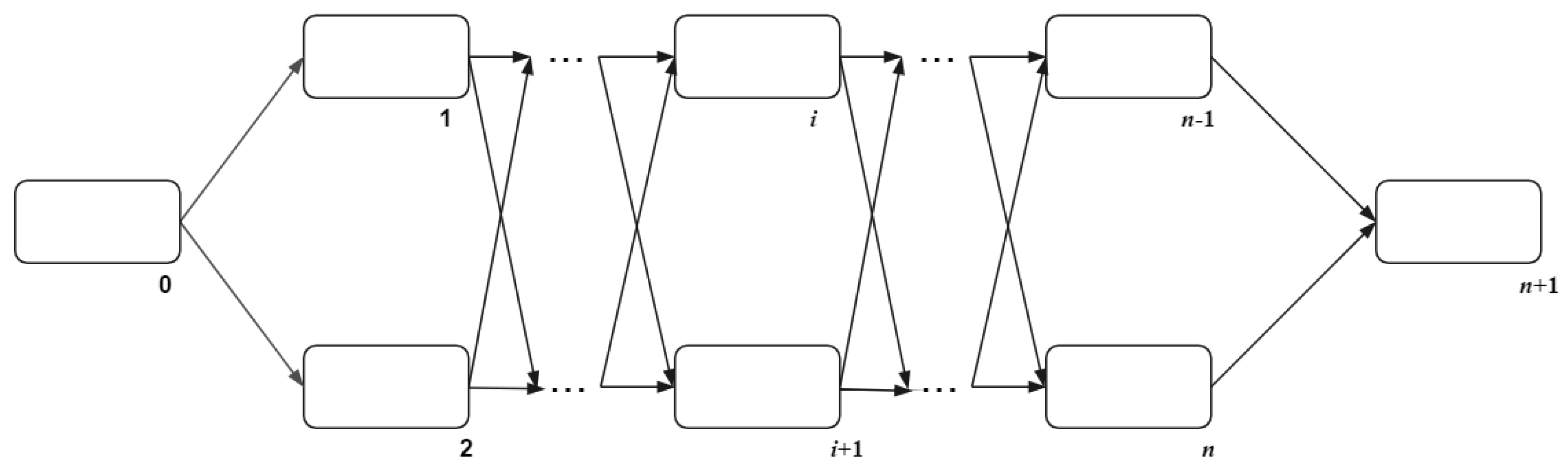
2.3.2. Tissue-Like P System

The tissue-like P system regards cells as the vertices of the graph in the system. The cells in the P system have different states, and the rules can be executed only when the required states are met. The basic membrane structure of the tissue-like P system is shown in Figure 2. Cell 0 is the input cell, which contains the initial object. The initial object uses rules and communication mechanisms to communicate in cell 1 to cell n. Cell n + 1 is the output cell, used to store the obtained results.

The formal definition of the traditional tissue-like P system is

$$\prod =(O,{\sigma }_1,\cdots ,{\sigma }_n,syn,i_{out})$$

where

• O is the alphabet, which contains all objects in the system;
• $syn\subseteq \{1,2,\cdots ,n\}\times \{1,2,\cdots ,n\}$ are synapses that connects cells;
• $i_{out}\in \{1,2,\dots ,n\}$ indicates the output cells of the system;
• ${\sigma }_1,\cdots ,{\sigma }_n$ represents n cells in the system, the detail definition are as follows:
• ${\sigma }_i=(Q_i,s_{i,0},w_{i,0},P_i),1\le i\le m$

where

(1)

$Q_i$ shows the collection of all states;

(2)

$s_{i,0}\in Q_i$ refers to the initial state;

(3)

$w_{i,0}\in O^{\ast }$ indicates the initial multiset of the object, when $w_{i,0}=\lambda$, there is no object in cell i;

(4)

$P_i$ stands for the rules of the entire system.

3. Noises Cutting and Natural Neighbors Spectral Clustering Based on Coupling P System

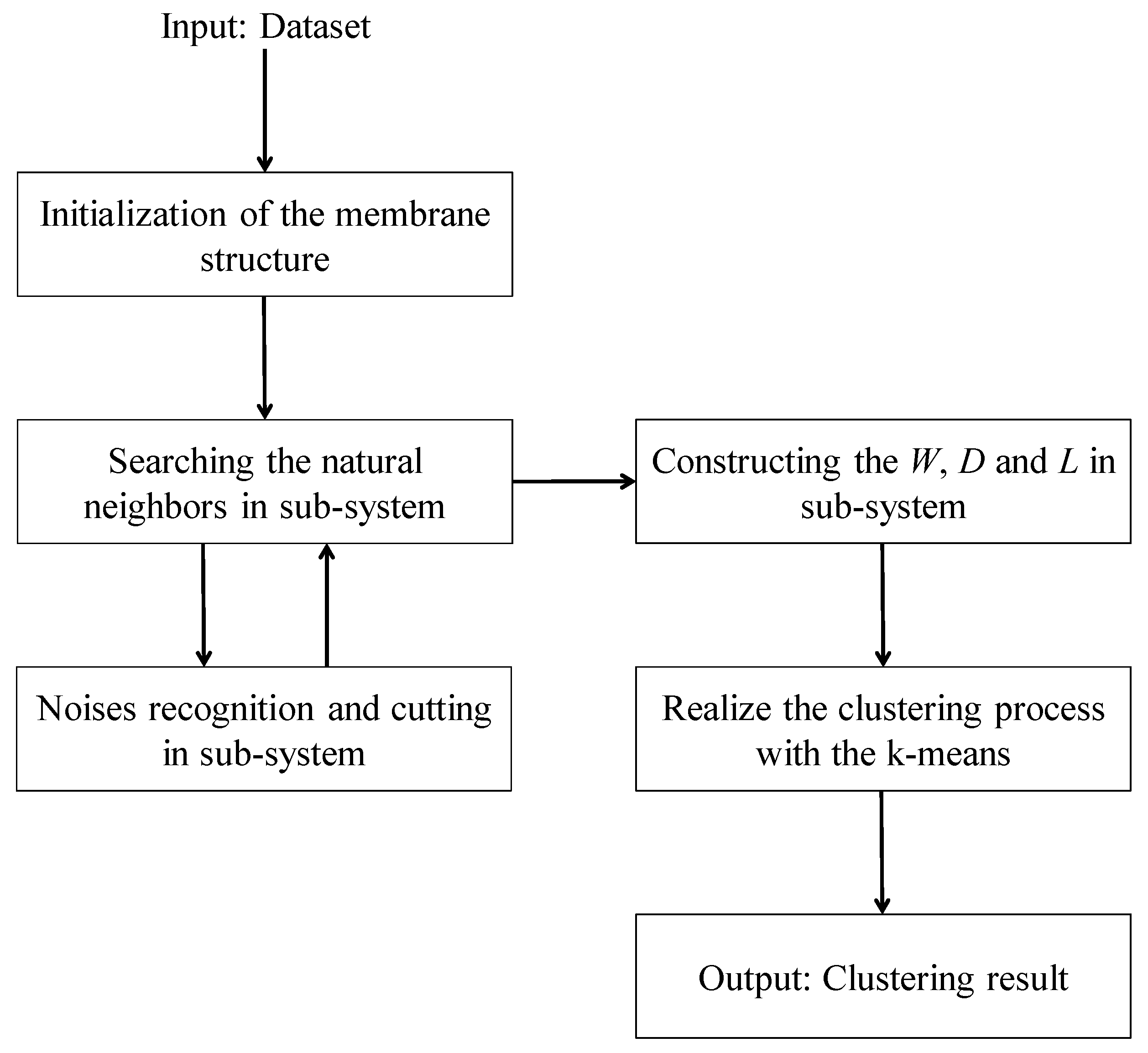
In this section, the spectral clustering method with noises cutting and the natural neighbors based on coupling P system is proposed. First, we explain the general framework of the coupling P system. Then, the different evolution rules and operations in the subsystems such as searching the natural neighbors, noises cutting, constructing affinity matrix, and clustering are introduced, respectively. Meanwhile, the communication rules between different membranes are elaborated. The flow chart of the proposed NCNNSC-CP algorithm is shown in Figure 3.

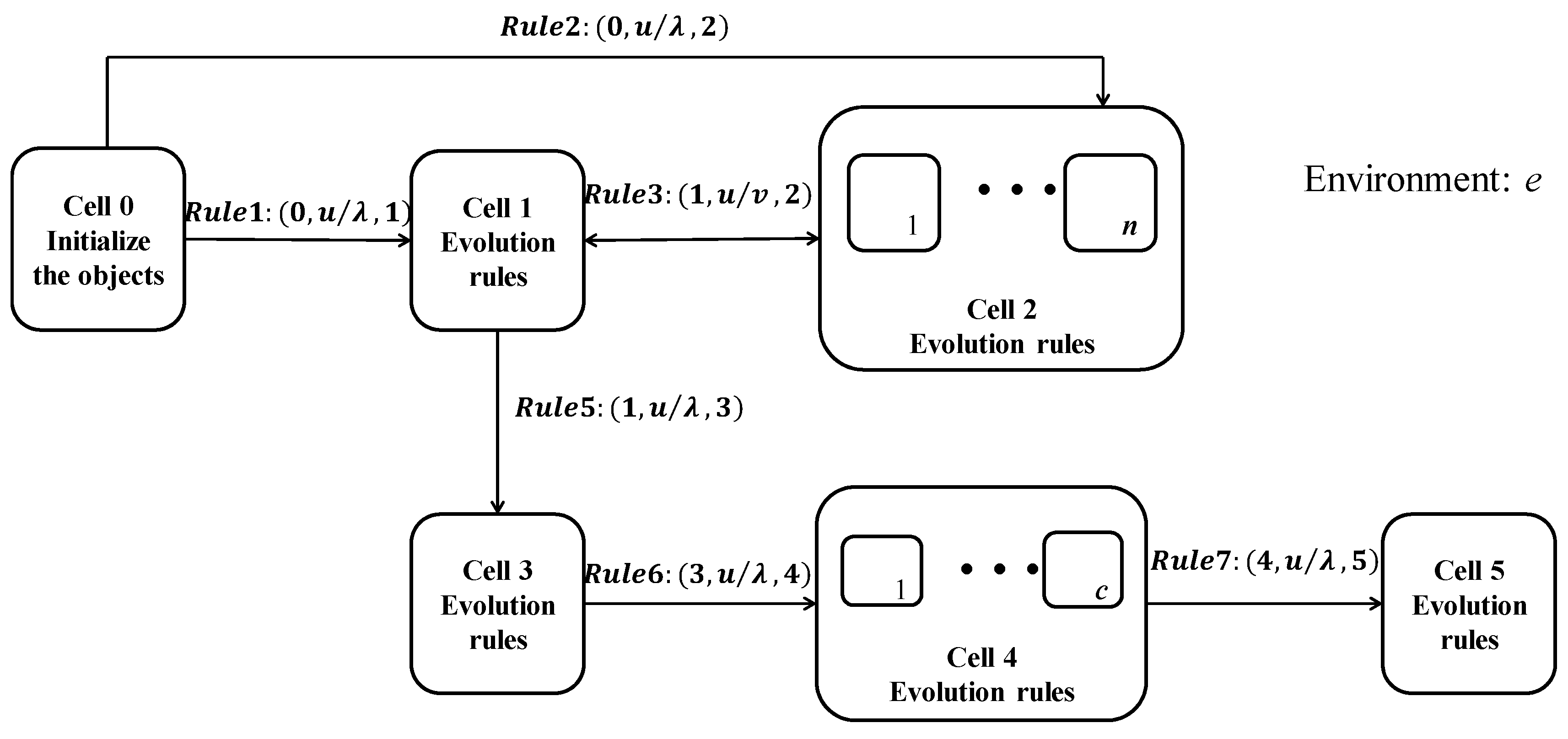
3.1. The General Framework of the Coupling P System

The proposed coupled P system (NCNNSC-CP) is the coupling of the cell-like P system and the tissue-like P system. According to the related concepts introduced in Section 2.3, the basic structure of the coupled P system is shown in Figure 4.

The formal definition of the coupled P system is

$$\prod =(O,\eta ,\mu ,syn,{\sigma }_0,\cdots ,{\sigma }_m,R,in,out)$$

where

• $O=\{x_1,x_{2,}\cdots ,x_n,d_{ij},NaN(x),Nb(x),Sup,Noises,c,w_{ij},D_{ii},L,\sigma \}$. x_i represents each data point. d_ij represents the distance between arbitrary two points. The natural neighbors of x denoted as NaN (x). Nb(x) refers to the number of reverse neighbors of x. Sup is the natural characteristic value. Noises stand for the noisy points in the dataset. c is the number of clusters. The similarity between data points x_i and x_j represented by w_ij. D_ii indicates the degree of data point x_i. L represents the Laplace matrix. $\sigma$ is the tuning parameters parameter.
• $\eta =\{x_1,x_{2,}\cdots ,x_n,\sigma ,c\}\in O$ represents the initial objects in the system.
• $\mu$ stands for the structure of the membrane.
• Syn = {{0,1},{0,2},{1,2}{1,3},{2,1},{3,4},{4,5}} means the synapses between cells. Its main function is to link cells so that they can communicate with each other.
• in is cell 0, the input membrane. out is cell 5, the output membrane.
• ${\sigma }_0,\cdots ,{\sigma }_m$ refers to cells in the system. The m is determined according to the number of clusters and the number of data points.
• R is the collection of rules, including communication rules and evolution rules.

Evolution rules are used to modify objects in the cluster, and communication rules are used to transfer objects from one cell to another.

3.2. The Evolution Rules

The rule R₀ for inputting cell is to transfer the raw dataset and the parameters to cell 1 for subsequent clustering algorithm operations. At the same time, the original data are transmitted to the cell 2 to perform noise cutting on the original data after the noises recognition. The specific R₀ rules can be described as

$$\begin{array}{l}{R}_{01}=\{x_1,\cdots ,x_n,c,\sigma \to x_1,\cdots ,x_n,c,\sigma {,}_{go{[]}_1}\}\\ R_{02}=\{x_1,\cdots ,x_n\to x_1,\cdots ,x_n{,}_{go{[]}_2}\}\end{array}$$

In terms of output cell 5, it is mainly used to store clustering results $R_5\ne \varnothing$.

3.2.1. The Evolution Rules of Searching the Natural Neighbors in Cell 1

The construction of affinity matrix can directly affect the clustering results of spectral clustering. In traditional algorithms, most of the parameters are determined based on artificial experience and manually input. According to the related concepts of natural neighbors and membrane system in Section 2, this paper uses the rules of searching natural neighbors without parameters in the membrane system to determine the natural characteristic value Sup and natural neighbors NaN(x).

In summary, the details rules of the evolution rules of The Natural Neighbors Searching (NaN-searching) in cell 1 are shown in rules R₁.

• R₁₁ (Sorting rule): Create a KD-tree T from the dataset D, which calculates the Euclidean distance of all points in the dataset D, and then sorts them in ascending order.
• R₁₂ (Searching rule): For each point x_i in D, we use a KD-tree T to find its rth neighbor x_j.
  Then, Nb(x_j) = Nb(x_i) + 1, $Na{N}_k(x_i)==Na{N}_{k-1}(x_i)\cup x_j;RN{N}_k(x_j)==Na{N}_{k-1}(x_j)\cup x_i$ according to Definition 2, Definition 3, and Equations (2) and (3) in cell 1. Finally, the natural neighbors of each point NaN(x) are transmitted to cell 2.
• R₁₃ (Iteration stop rule): When the number of x_i’s reverse neighbors Nb(x_i) no longer changes or is always equal to 0, evolution stops.
• R₁₄ (Determining the natural characteristic value Sup rule): the natural characteristic value Sup is calculated by Equation (4) in the cell 1. Then, transmitted the Sup to cell 2.

Apparently, the search of natural neighbors is different from the traditional k-nearest method. The k nearest neighbors of each point x_i can be found without any parameters in the whole algorithm process in cell 1.

3.2.2. The Evolution Rules of Noises Recognition and Cutting in Cell 2

In cell 2, we execute the evolutionary rules of noises recognition and cutting.

Noise points refer to data with errors or anomalies (deviations from expected values) in the data, which are neither core points nor boundary points in the data set. At the same time, these noises cause great interference to the data analysis and preprocessing, especially for clustering, which is extremely sensitive to them based on empirical data. Therefore, it is particularly significant to identify and eliminate noise points. Jokinen et al. [6] deal with noise on the basis of spatial clustering based on hierarchical density, and proposes a density-based cluster ability measure. We propose a noise recognition and cutting method based on the reverse density and critical reverse density in natural neighbors. The reverse density and critical reverse density are specifically defined as follows.

Definition 6:

(Reverse density).Based on the natural neighbors NaN(x_i) of the data object x_i, we define the inverse density as the average distance between x_i and all its natural neighbors:

$$Rd(x_i)=\frac{1}{Sup}{\displaystyle \sum _{x_j\in NaN(x_i)}d(x_i,x_j)}$$

(5)

Definition 7:

(Critical Reverse density).The critical reverse density of point x_i is calculated from the average reverse density Rd(x_i) and the standard deviation of the reverse density std(Rd(x_i)) of all objects in the data set D:

$$CRd(x_i)=mean(Rd(x))+\alpha \cdot std(Rd(x))(\forall x\in D)$$

(6)

where$\alpha$is a tuning coefficient, and experiments show that a = 1 is suitable for most data sets.

Definition 8:

(Noises).If the x_i’s reverse density is larger than its critical inverse density, it is a noise point.

$$Noises=\left\{x\right|\forall x\in D,Rd(x)>CRd(x)\}$$

(7)

In accordance with the natural neighbors of point x obtained in cell 1 and the above concepts, we simultaneously conduct noise recognition for all points in the n sub-cells of cell 2. This step is parallel to improve computational efficiency. When it is judged that x is a noise, it is transported to the environment outside the cell 2 and discard x. The details rules of the evolution rules of Noises Recognition and Cutting (Noises-rc) in cell 2 are shown in rules R₂.

• R₂₁ (Noise recognition rule): For each point x_i in D, using Equation (6) to get Rd(x) and then using Equation (7) to get CRd(x) in sub-cells of cell 2.
• R₂₂ (Noise cutting rule): For each point x_i in D, if the object x_i satisfies the Equation (8) it will be transmitted from the cell 2 to the environment. Otherwise, the rest of the data is sent to cell 1.

3.2.3. The Evolution Rules of Constructing the Affinity Matrix, Degree Matrix and Laplacian Matrix in Cell 3

In spectral clustering, the construction of affinity matrix plays an important role in the clustering result. Generally, it is obtained by calculating the Gaussian kernel distance between the data point x_i and its natural neighbors. However, due to the influence of noise points, the natural neighbors of the data points are mixed with noises, which is not conducive to the construction of the affinity matrix. Relatively speaking, noise identification and screening based on reverse density and critical reverse density are extremely effective. The data set D’ is deduced through the Section 3.2.2 which is the core data set. Therefore, we perform the natural neighbor searching again to acquire the core natural neighbor of the data object. Although it will increase the complexity of the algorithm to a certain extent, it is worthwhile compared with the greatly improved accuracy. The core natural neighbor is defined as follows.

Definition 9:

(The Core Natural Neighbors).For each object x in dataset D, its core natural neighbors are k nearest neighbors without noises, denoted as CNaN (x).

At last, we perform spectral clustering (NJW [28]). On the basis of the affinity matrix W, we calculate the degree matrix D:

$$D_{ii}={\displaystyle {\sum }_{j=1}^n{W}_{ij}}$$

(8)

As for the Laplacian matrix L, we utilize the Symmetric normalized Laplacian matrix:

$$L=I-D^{-1/2}W{D}^{-1/2}$$

(9)

Next, we choose the eigenvector $u_1,u_2,\cdots u_c$ corresponding to the first k eigenvalues of the L to comprise $U=\{u_1,u_2,\cdots u_c\},U\in R^{n\ast c}$, and standardize it by row to get Y:

$$Y_{ij}=U_{ij}/{({\displaystyle {\sum }_j{U}_{ij}^2})}^{1/2}$$

(10)

The details rules of the evolution rules of constructing the Affinity Matrix, Degree Matrix, and Laplace matrix in cell 3 are shown in rules R₃.

• R₃₁ (Constructing the affinity matrix rule): Based on the core natural neighbors CNaN (x) and the input parameters, the affinity matrix W is calculated in cell 3. For the jth natural neighbor in CNaN(x_i) of x_i, $W_{ij}=\exp (d{(i,j)}^2/2{\sigma }^2)$. Moreover, If W_ij is a real number while W_ji is equal to 0, the value of W_ij is assigned to W_ji by the principle of symmetry.
• R₃₂ (Constructing the degree matrix rule): According as the affinity matrix and the Equation (8), the degree matrix is obtained in cell 3.
• R₃₃ (Constructing the Laplacian matrix rule): As for the Laplacian matrix L, we utilize the Symmetric normalized Laplacian matrix using Equation (9) in cell 3.
• R₃₄ (Constructing novel cluster sample): Based on the above concepts and Equation (10), we construct the Y in cell 3 for the next step of clustering. Each row of Y represents a sample. Simultaneously, it is transmitted into cell 4.

3.2.4. The Evolution Rules of K-Means (Clustering Method)

In the last step of NCNNSC-CP, the K-means is applied to cluster the new samples into clusters $C_1,C_2,\cdots C_c$. In cell 4, there are k sub-cells running simultaneously.

The details rules of the evolution rules of K-means are shown in rules R₄.

• R₄₁ (Random selection of cluster center rule): Randomly selecting c points from the dataset as the initial cluster centers and store them in c sub-cells.
• R₄₂ (Clustering rule): The distance between each sample point and each cluster center in sub-cell is calculated and transmitted to cell 4. Then, the data points are clustered according to the principle of nearest distance in cell 4.
• R₄₃ (Redefine the cluster center rule): According to each cluster divided by rule R42, the average distance of each cluster is calculated to change the cluster center. If the cluster center changes, the clustering process are repeated. Otherwise, the cluster result $C_1,C_2,\cdots C_c$ is output to cell 5.

3.3. The Communication Rules between Different Cells

Communication between cells in the CP system can only be achieved when there is a synapse between different cells. In order to ensure the effectiveness of the system and improve the efficiency of the system, this paper constructs a CP system with directional communication rules. In the CP system, some membranes are responsible for initializing objects and outputting results, and some membranes are responsible for algorithm execution. Orderly communication between different membranes makes the whole algorithm more effective.

There are three communication rules in the CP system: one-way transmission and two-way transmission between cells and one-way transmission between cells and the environment.

(1) One-way transmission between cells includes Rule1, Rule2, Rule5, Rule6, and Rule7. $\lambda$ is null.

• $Rule1:(0,u/\lambda ,1)$ It can transfer the string u including the original data and parameters from cell 0 to cell 1.
• $Rule2:(0,u/\lambda ,2)$ The original data string u can be sent to cell 2 from cell 1It can transfer the string u including the original data and parameter $\alpha$ from cell 0 to cell 2.
• $Rule5:(1,u/\lambda ,3)$ It can transmit the strings u of the natural neighbors, natural characteristic value, and related parameter strings of the dataset in cell 1 to cell 3.
• $Rule6:(3,u/\lambda ,4)$ The strings u of new sample data and related parameter generated in cell 3 are transported to cell 4.
• $Rule7:(4,u/\lambda ,5)$ The clustering results generated in cell 4 are transferred to cell 5 for storage.

(2) Two-way transmission between cells is Rule3.

• $Rule3:(1,u/v,2)$ It can transfer the string u of the natural neighbors and the natural characteristic in cell 2 to cell 3, and transfer the dataset without noises υ in cell 3 to cell 2.

(3) One-way transmission between cell and the environment is Rule4.

• $Rule4:(2,u/\lambda ,e)$ The noise data u generated in cell 2 is transferred to environment e and discarded.

3.4. Computational Complexity

We assume that n is the total number of points in the dataset. The time complexity of NCNNSC-CP algorithm can be calculated as follows. (1) The time complexity for searching the natural neighbors is O(nlogn). (2) Noise recognition and cutting require O(n). (3) Constructing the Affinity Matrix requires O(n²). (4) Eigenvalue decomposition requires O(n³). (5) Clustering by K-means requires O(n). To sum up, the overall complexity of the proposed clustering method NCNNSC-CP is O(n³).

4. Experiments Analysis

4.1. Experimental Setting

All experiments were conducted in Matlab 2016a on a PC with Intel core i5-940M CPU, 4GB RAM, Windows 7 64-bit operating system. In the section, we conduct experiments on synthetic data sets and real data sets to evaluate the performance of the proposed NCNNSC-CP method. At the same time, we compare it with state-of-the-art clustering methods, including K-means [32], DBSCAN [33], DPC [34], Cut-PC [35], SC [29], U-SPEC (Ultra-Scalable Spectral Clustering) [15], U-SENC (Ultra-Scalable Ensemble Clustering) [15], and NNSC, for comparative analysis.

4.2. Evaluation Metrics

In order to measure the quality of the clustering results, external indicators have been usually used in the clustering validity indexes. This paper uses 4 commonly used clustering indicators—accuracy (Acc), F1-measure, Normalized Mutual Information (NMI), and Adjusted Rand Index (ARI)—to evaluate clustering performance, which has been advocated and discussed [36].

(1) Acc: Accuracy indicates the ratio of the number of samples with correct clustering to the total number of samples, where P is the predicted label and T is the true label.

$$Acc=\frac{{\displaystyle \sum _{i=1}^k\underset{j}{\max |p_i\cap t_j|}}}{N}$$

(11)

(2) ARI: Rand Index represents the degree of similarity between the predicted value and the actual value of the sample, and its range is [0, 1]. However, for random results, RI does not guarantee that the score is close to 0, so the Adjusted Rand Index with higher discrimination is proposed. The value range is [−1, 1]. The larger the value, the more consistent the clustering result is with the real situation.

$$RI=\frac{TP+TN}{TP+FP+TN+FN}$$

(12)

$$ARI=\frac{RI-E[RI]}{\max (RI)-E[RI]}$$

(13)

where TP, FP, TN, and FN represent true positive, false positive, true negative, and false negative decisions, respectively.

(3) F1-measure: The F1-measure is the harmonic mean of precision and recall, and it is a commonly used comprehensive evaluation index in clustering. The Precision indicates the proportion of samples classified as positive samples that are actually positive samples. The Recall rate refers to the proportion of instances that are actually classified as positive instances.

$$F=\frac{2\ast P\ast R}{P+R}$$

(14)

$$P=\frac{TP}{TP+FP}$$

(15)

$$R=\frac{TP}{TP+FN}$$

(16)

(4) NMI: Normalized Mutual Information utilized information theory to measure the differences between the clustering partitions and its range is in [0, 1].

$$NMI(X;Y)=2\frac{I(X;Y)}{H(X)+H(Y)}$$

(17)

where I(X;Y) is the mutual information between X and Y, and H(X), H(Y) are the entropy of random variables.

4.3. Experiments on Synthetic Datasets

Table 1. The basic information of the nine synthetic data sets.

Dataset	Objects	Attributes	Clusters
D1	513	2	5
D2	420	2	2
D3	1532	2	2
D4	3883	2	3
D5	1114	2	4
D6	1064	2	2
D7	1915	2	6
D8	1427	2	4
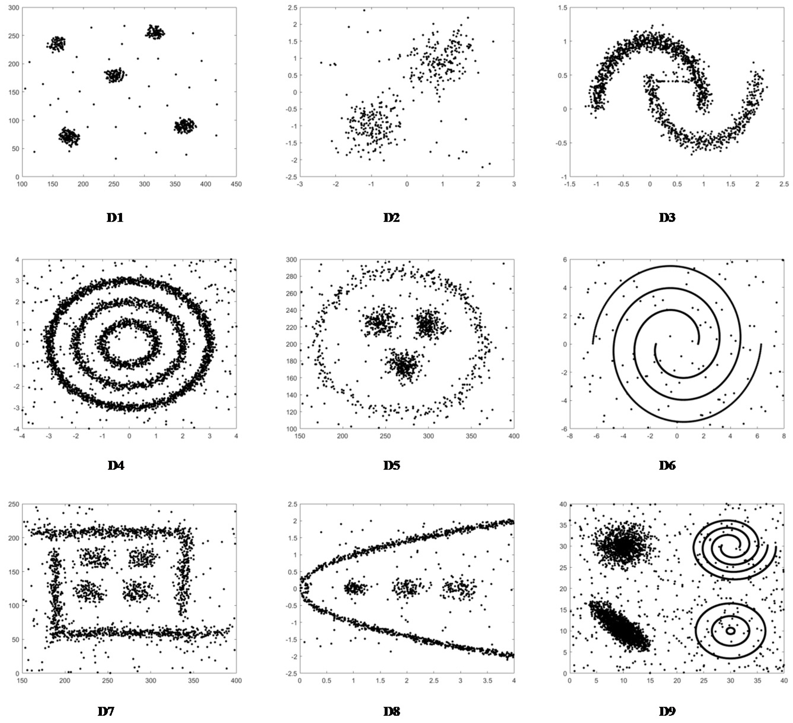
D9	8533	2	7

shows the basic information of the nine synthetic data sets. The original data of the nine synthetic data sets are shown in Figure 5.

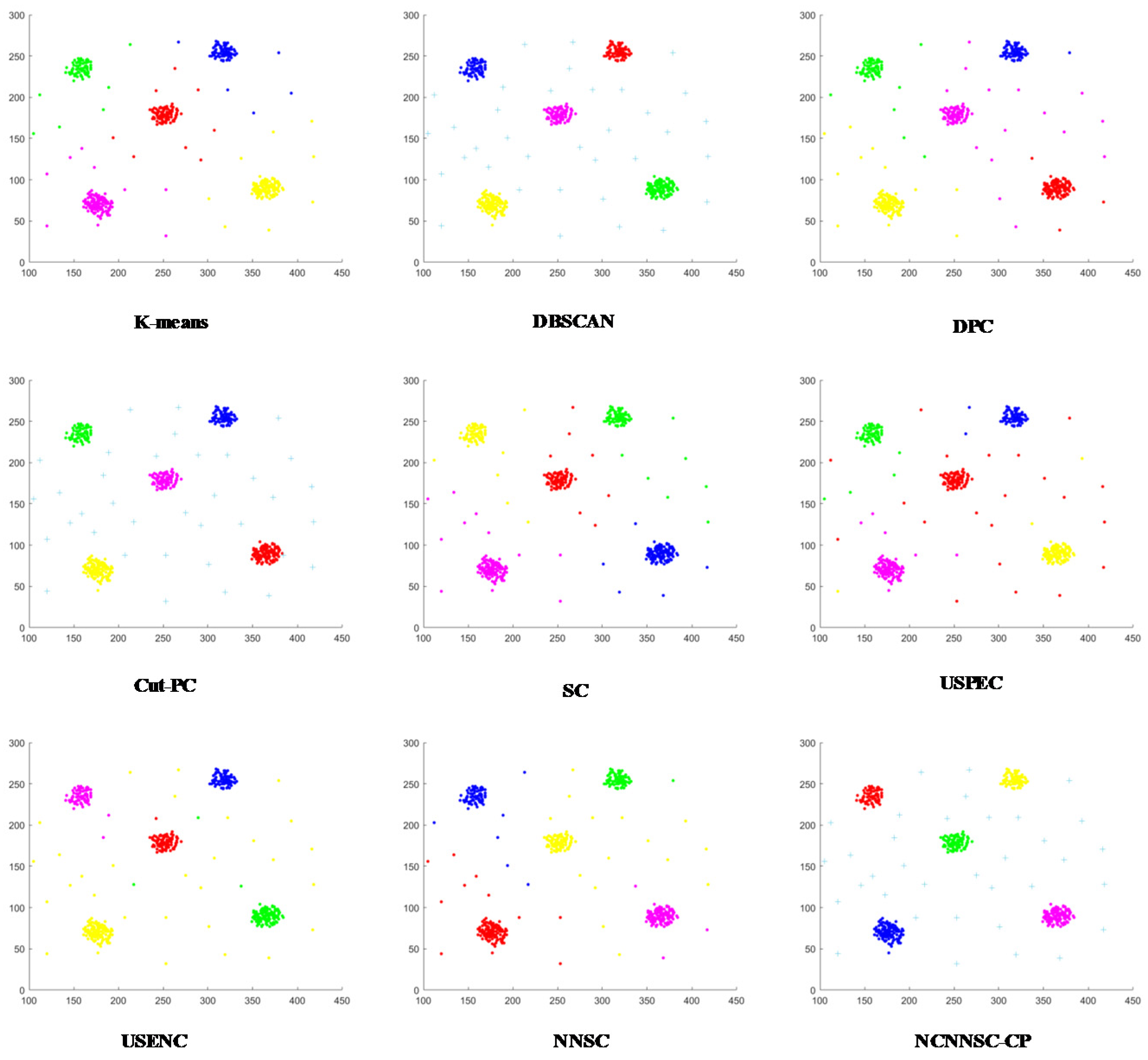
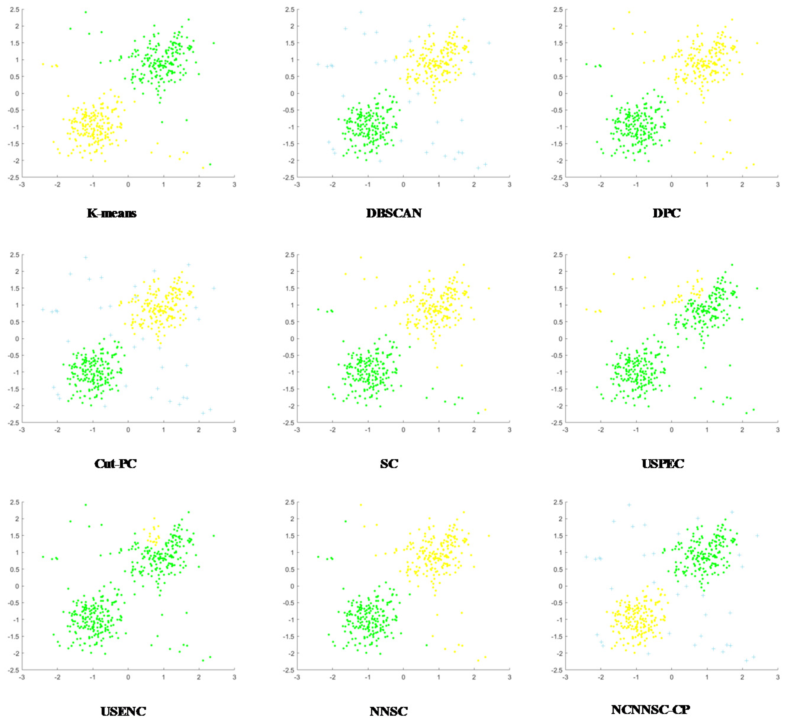
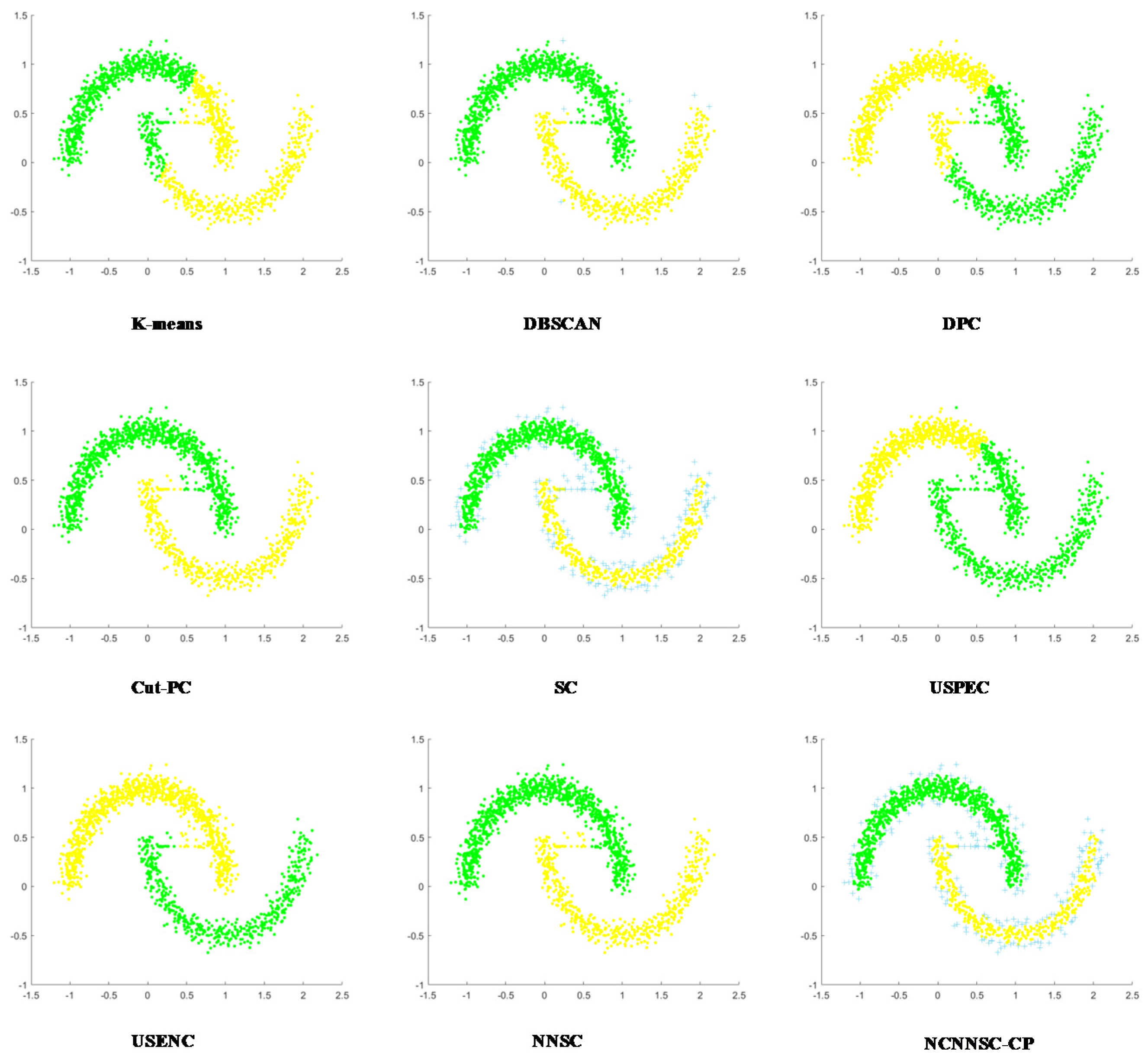
Figure 6 shows that all clustering methods have good clustering performance on the D1 dataset. It can be seen from Figure 7 that in addition to the USENC and USPEC algorithms, other clustering methods work well on the D2 dataset. This may be because USENC and USPEC are more focused on clustering of very Ultra-scale data sets with limited resources. As shown in Figure 8, only the DPC, K-means, and USENC methods are not effective for the D3 dataset. In fact, DPC and K-means cannot detect non-spherical clusters.

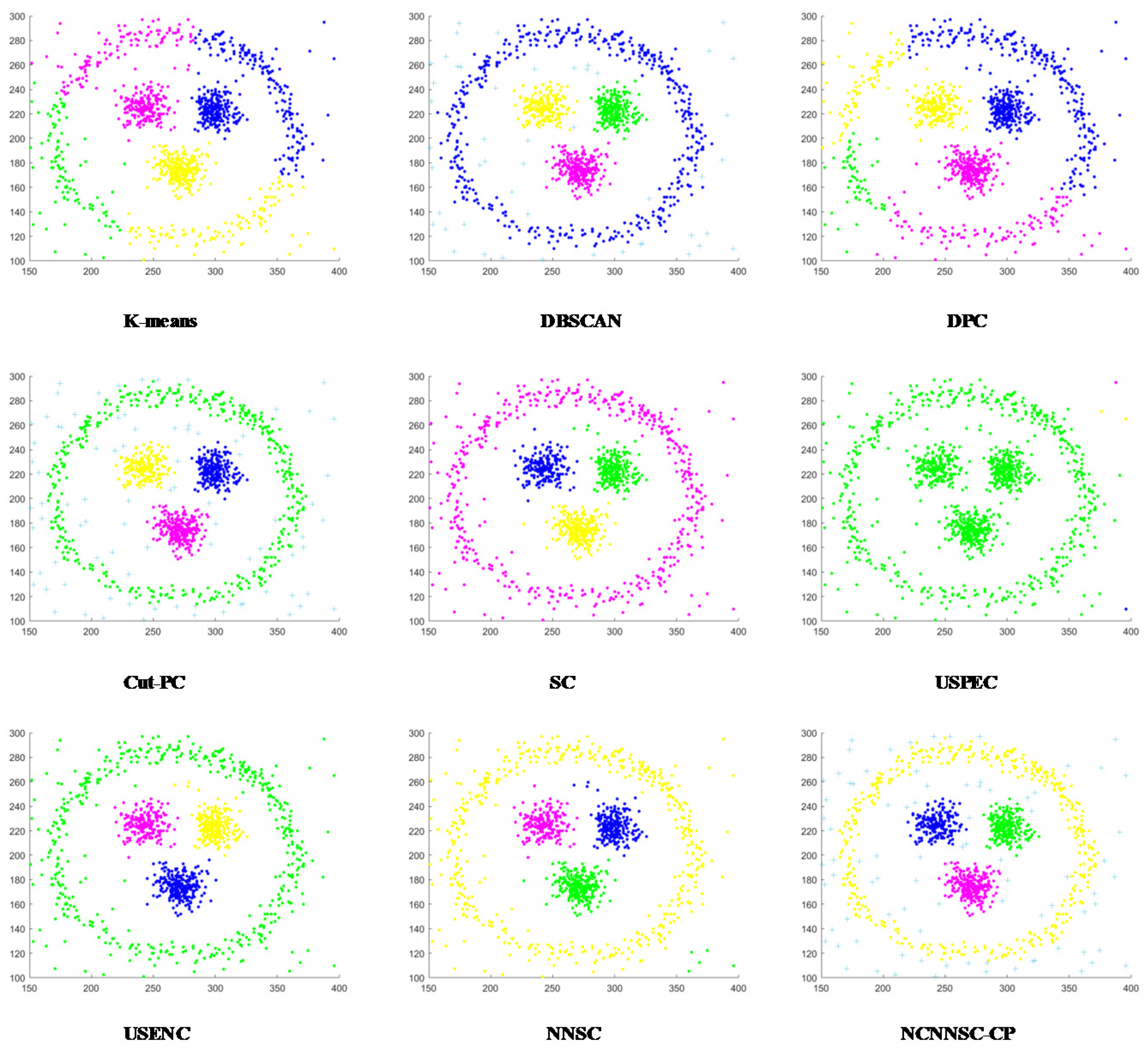
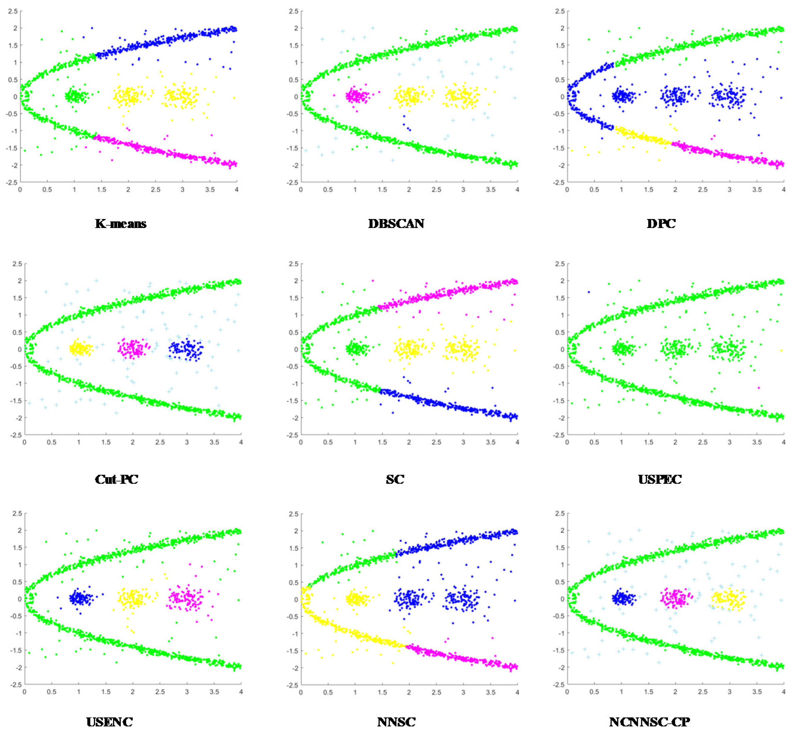
The clustering results in Figure 9 demonstrate that DBSCAN, Cut-PC, USENC, and NCNNSC algorithms can cluster D4 well. Although k-means, DPC, SC, and NNSC perform well on the spherical cluster dataset, they cannot handle circular clusters. USPEC algorithms performed the worst. It can be seen from Figure 10 that most of the algorithms can perform clustering excellently on the D5 dataset. However, DPC, K-means, and USPEC are not well recognized, which again proves that DPC and K-means cannot handle circular clusters well.

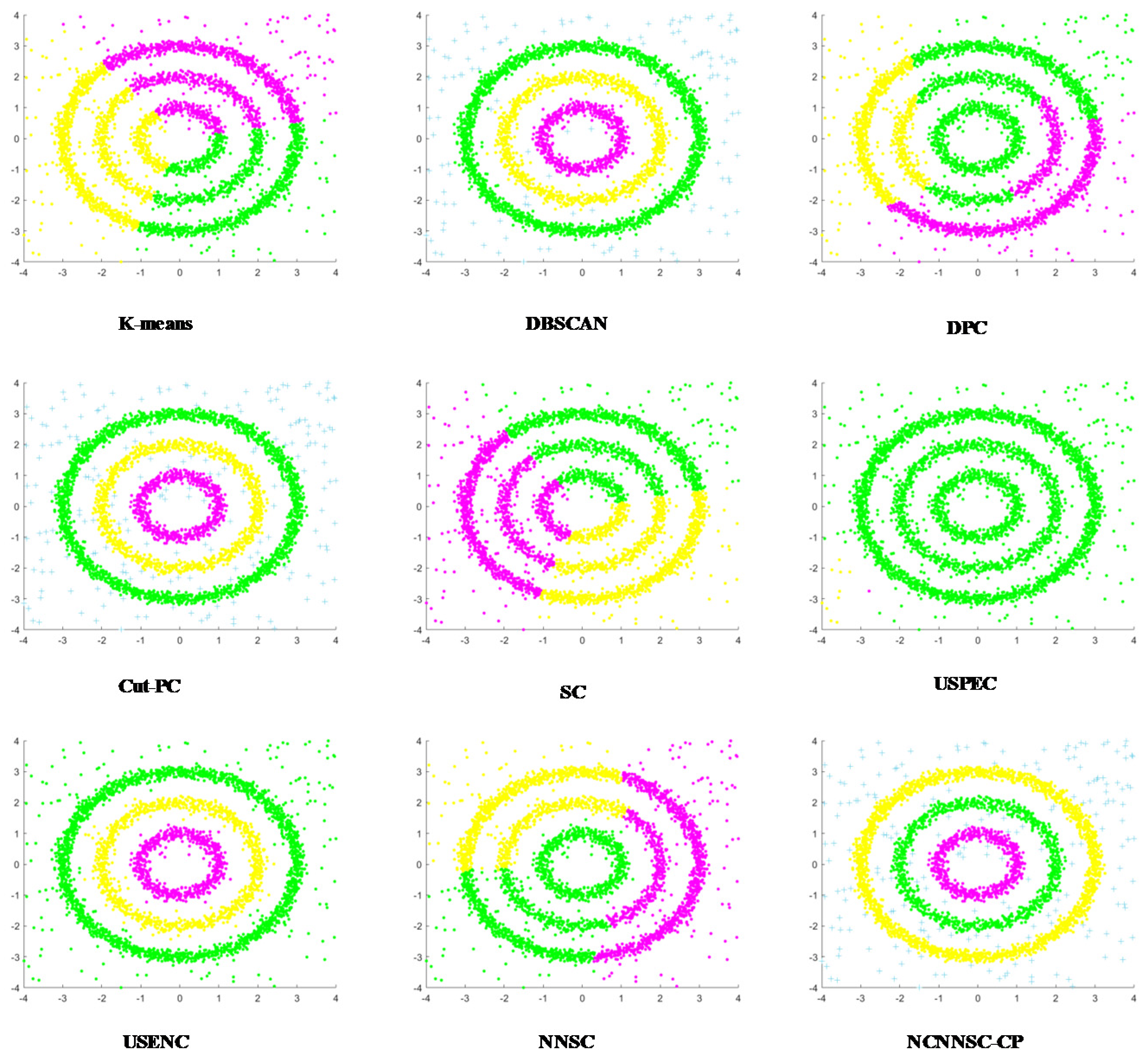
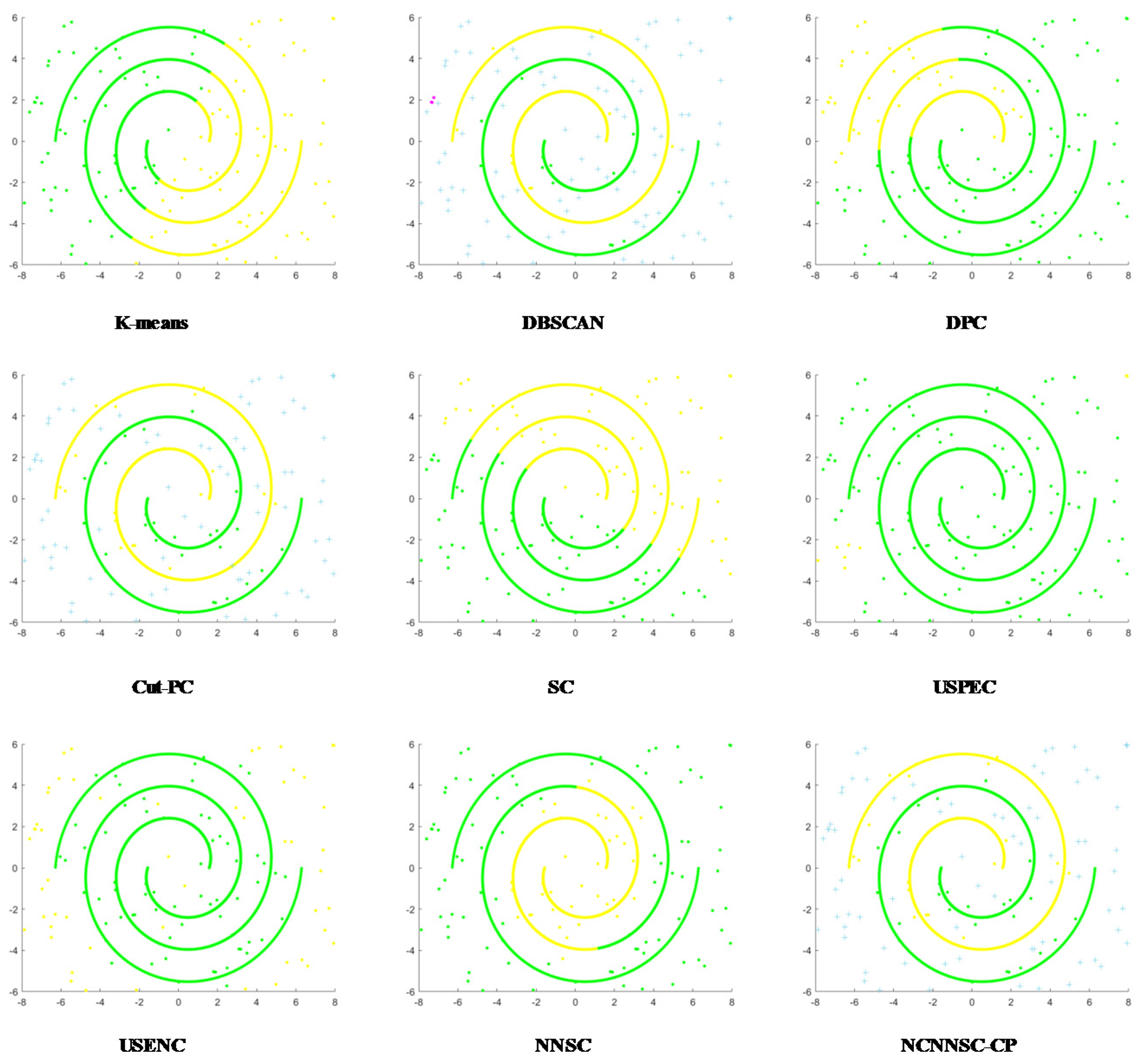
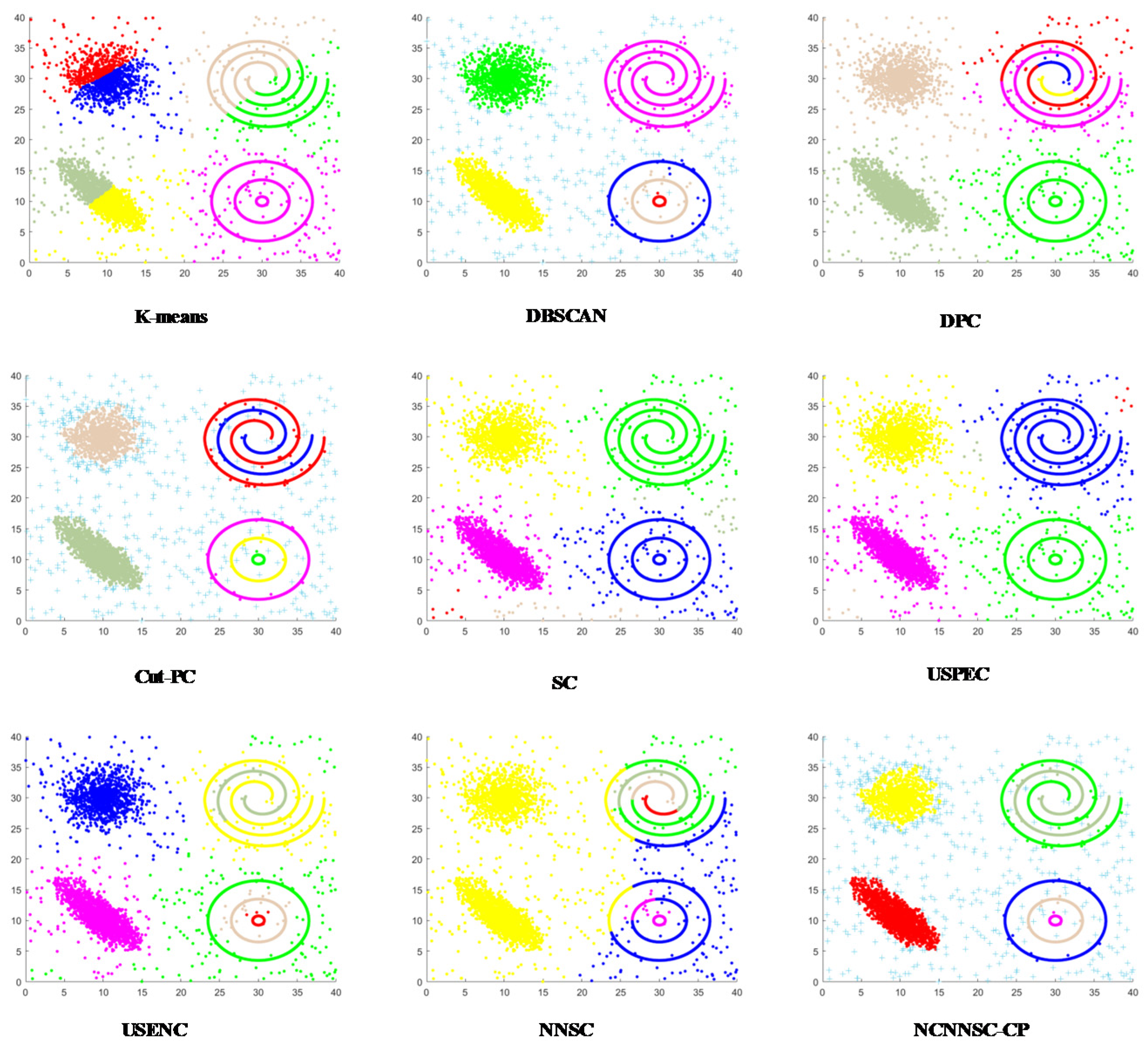
Figure 11 illustrates that DBSCAN, Cut-PC, and NN-NCSC are processed well for clusters of spiral clusters. The similarity is that these three algorithms have been processed with noise. Generally, SC can handle spiral clusters well, but part of the data in this dataset is too scattered, which affects the final clustering performance. As shown in Figure 12, only DBSCAN, USENC, and NCNNSC-CP have good clustering results for the data set D7. SC and Cut-PC achieved similar results. Other algorithms are less efficient.

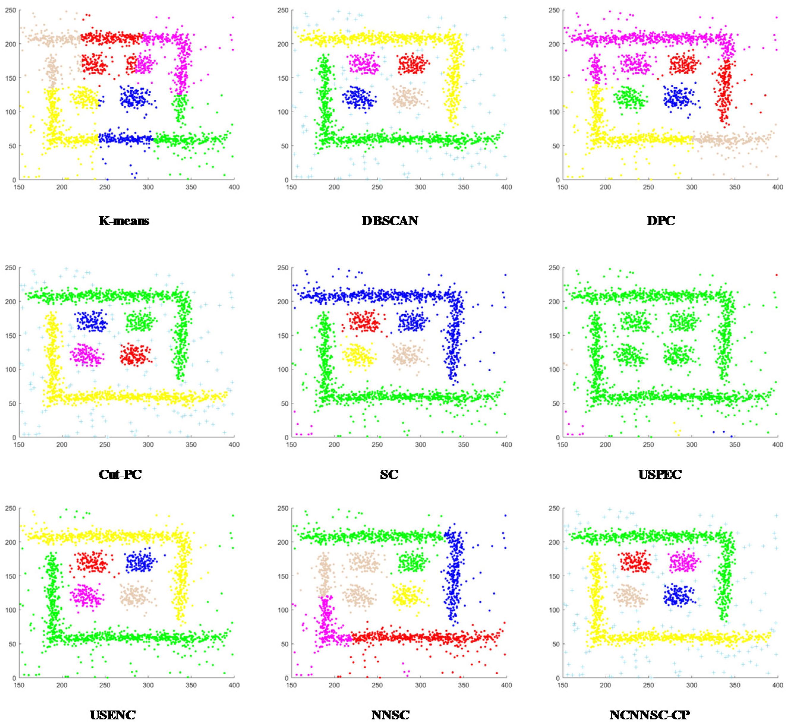
From the clustering shown in Figure 13, Cut-PC, USENC, and NCNNSC-CP can identify clusters in the D8 dataset, while other algorithms cannot. As for the last data set D9, which is displayed in Figure 14, only Cut-PC and NCNNSC-CP clustered it correctly. The USENC clustering results are almost correct but there are some deviations. The clustering results of SC and USPEC are similar, and most of the data are classified into four categories. For other algorithms, the clustering results are very poor. Therefore, NCNNSC-CP algorithms can effectively detect irregular data sets.

In conclusion, the NCNNSC-CP algorithm performs better than other algorithms from Figure 2, Figure 3, Figure 4, Figure 5, Figure 6, Figure 7, Figure 8, Figure 9 and Figure 10 and can properly recognize different types of clusters. Simultaneously, it can achieve effective clustering results on data sets of different scales and can be applied to more complicated situations.

4.4. Experiments on Real Datasets

The UCI data set is a commonly used standard test data set, which is often used in many clustering experiments. In this paper, we conduct experiments on six real UCI data sets. The specific information is shown in

Table 2. The basic information of the six UCI data sets.

Dataset	Objects	Attributes	Clusters
Iris	150	4	2
Seeds	210	6	3
Breastcancer	699	9	2
Banknote	1372	4	2
Thyroid	215	5	3
Ionosphere	351	34	2

. For the parameter setting of different algorithms, we conduct 20 iterations of experiments for each algorithm. The results of ACC, ARI, F, and NMI of the nine algorithms on the six UCI data sets are given in

Table 3. The Accuracy of the nine algorithms on six UCI datasets.

Dataset	K-Means	DBSCAN	DPC	Cut-PC	SC	USPEC	USENC	NNSC	NCNNSC-CP
Iris	0.8933	0.9267	0.9067	0.7000	0.9067	0.9467 *	0.9067	0.9000	0.9683
Seeds	0.8905	0.8048	0.8857	0.4978	0.8905	0.6476	0.8095 *	0.8381	0.9355
Breastcancer	0.9585	0.9628	0.6552	0.8526	0.9557	0.6567	0.9714 *	0.9614	0.9739
Banknote	0.6122	0.9628	0.7413	0.9308	0.6851	0.8528	0.8593	0.8958	0.9325*
Thyroid	0.8058	0.6977	0.7209	0.8000	0.7907 *	0.7070	0.8000	0.7302	0.9018
Ionosphere	0.7094	0.8319	0.6410	0.8234 *	0.7094	0.6439	0.7094	0.8091	0.9091

Bold shows the best result. Asterisk (*) refers to the second-best result.

,

Table 4. The ARI of the nine algorithms on six UCI datasets.

Dataset	K-Means	DBSCAN	DPC	Cut-PC	SC	USPEC	USENC	NNSC	NCNNSC-CP
Iris	0.7302	0.6841	0.7592	0.4819	0.7583	0.8512 *	0.7592	0.7445	0.9128
Seeds	0.7103 *	0.2163	0.7027	0.3667	0.7054	0.4402	0.5543	0.6065	0.8152
Breastcancer	0.8391	0.7509	0.0939	0.4829	0.8285	0.0026	0.8879	0.8499	0.8736 *
Banknote	0.0485	0.0296	0.2308	0.4045	0.1310	0.4974	0.5161	0.6262 *	0.7480
Thyroid	0.4016	0.0165	0.1316	0.4474 *	0.3752	0.0313	0.4523	0.1114	0.4324
Ionosphere	0.1728	0.2544	0.0000	0.3987	0.1727	0.0045	0.1726	0.3517 *	0.1953

Bold shows the best result. Asterisk (*) refers to the second-best result.

,

Table 5. The F-measure of the nine algorithms on six UCI datasets.

Dataset	K-Means	DBSCAN	DPC	Cut-PC	SC	USPEC	USENC	NNSC	NCNNSC-CP
Iris	0.8918	0.8667	0.9048	0.7277	0.9053	0.9465 *	0.9048	0.8983	0.9683
Seeds	0.8897	0.5608	0.8822	0.0025	0.8907 *	0.7303	0.8071	0.8360	0.9353
Breastcancer	0.9584	0.8741	0.6623	0.8444	0.9555	0.6954	0.9716 *	0.9614	0.9739
Banknote	0.6026	0.2484	0.7311	0.7648	0.6453	0.8532	0.8597	0.8958 *	0.9325
Thyroid	0.7734	0.5985	0.6252	0.7682	0.7356	0.6547	0.8016 *	0.6714	0.8535
Ionosphere	0.7149	0.7456	0.6228	0.8062*	0.7148	0.6902	0.7147	0.7758	0.8738

Bold shows the best result. Asterisk (*) refers to the second-best result.

and

Table 6. The Normalized Mutual Information (NMI) of the nine algorithms on six UCI datasets.

Dataset	K-Means	DBSCAN	DPC	Cut-PC	SC	USPEC	USENC	NNSC	NCNNSC-CP
Iris	0.7582	0.6986	0.8057	0.5530	0.7857	0.8449 *	0.8057	0.7777	0.9043
Seeds	0.7101 *	0.4095	0.6982	0.4815	0.6869	0.5372	0.6204	0.6560	0.7736
Breastcancer	0.7361	0.5965	0.1089	0.3909	0.7219	0.0047	0.8138	0.7492	0.7501 *
Banknote	0.0303	0.2305	0.3464	0.4566	0.2120	0.4103	0.4328	0.6111 *	0.6420
Thyroid	0.3428	0.2224	0.1786	0.3832	0.3397	0.0422	0.3208	0.1376	0.3815 *
Ionosphere	0.1320	0.2950	0.0699	0.3810	0.1299	0.0087	0.1278	0.3237*	0.1644

Bold shows the best result. Asterisk (*) refers to the second-best result.

, respectively. The best results are shown in bold, and the second best are shown in asterisks (*).

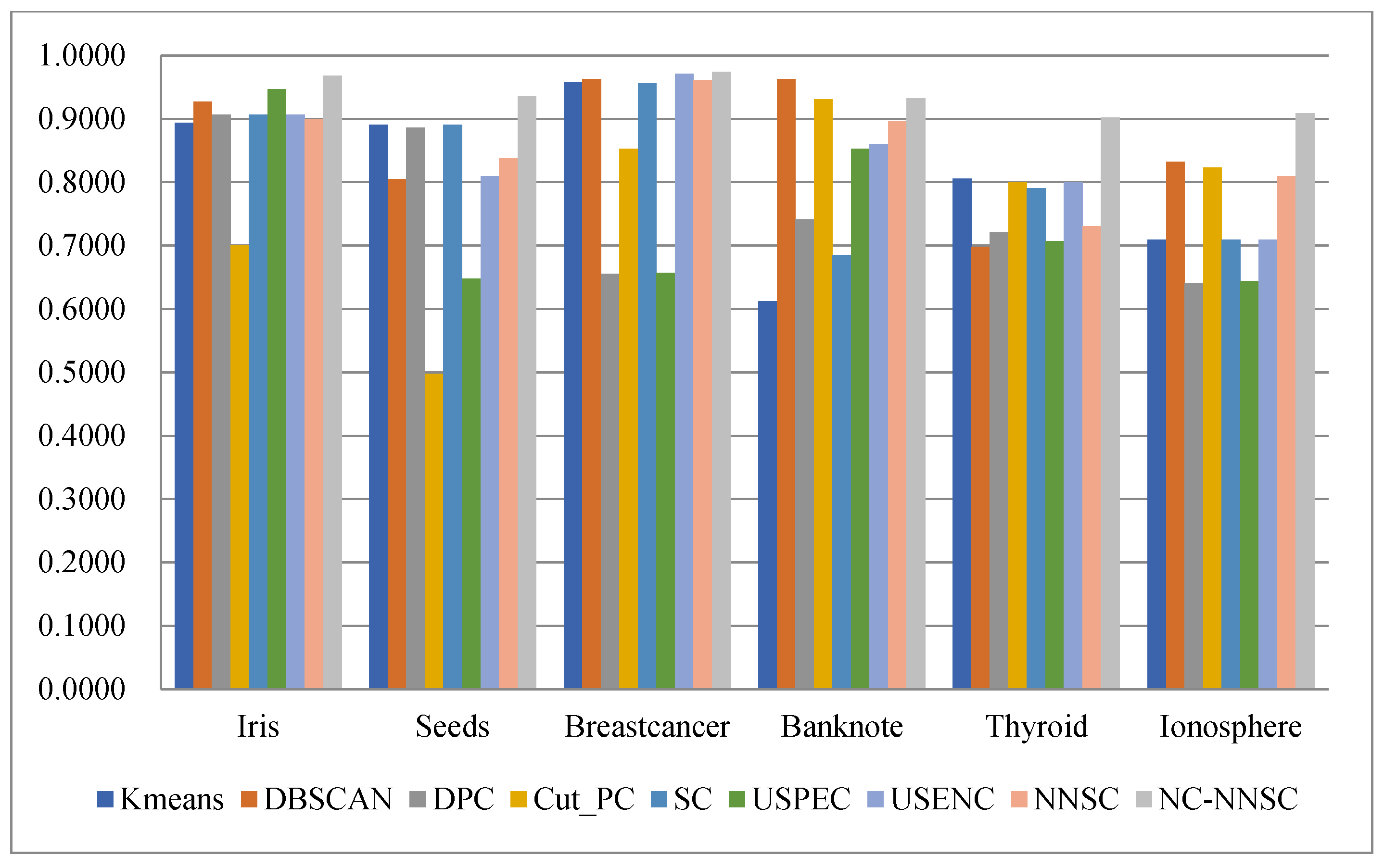
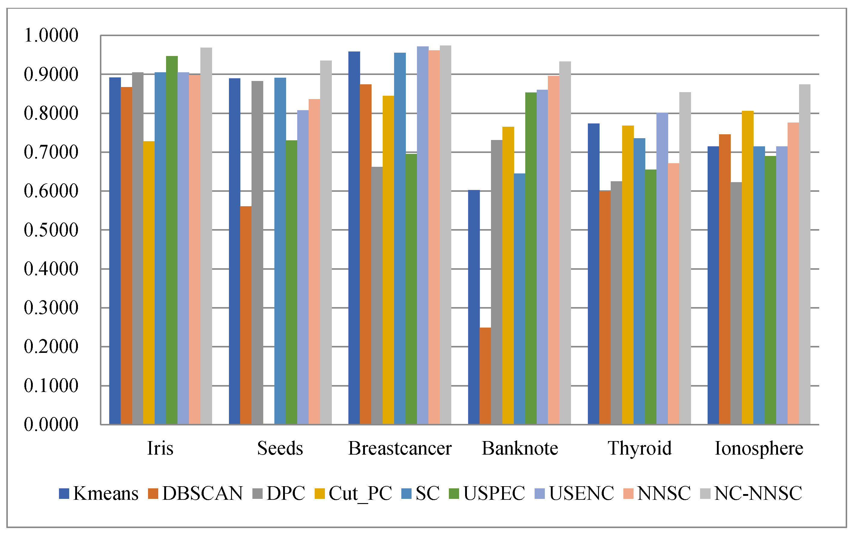
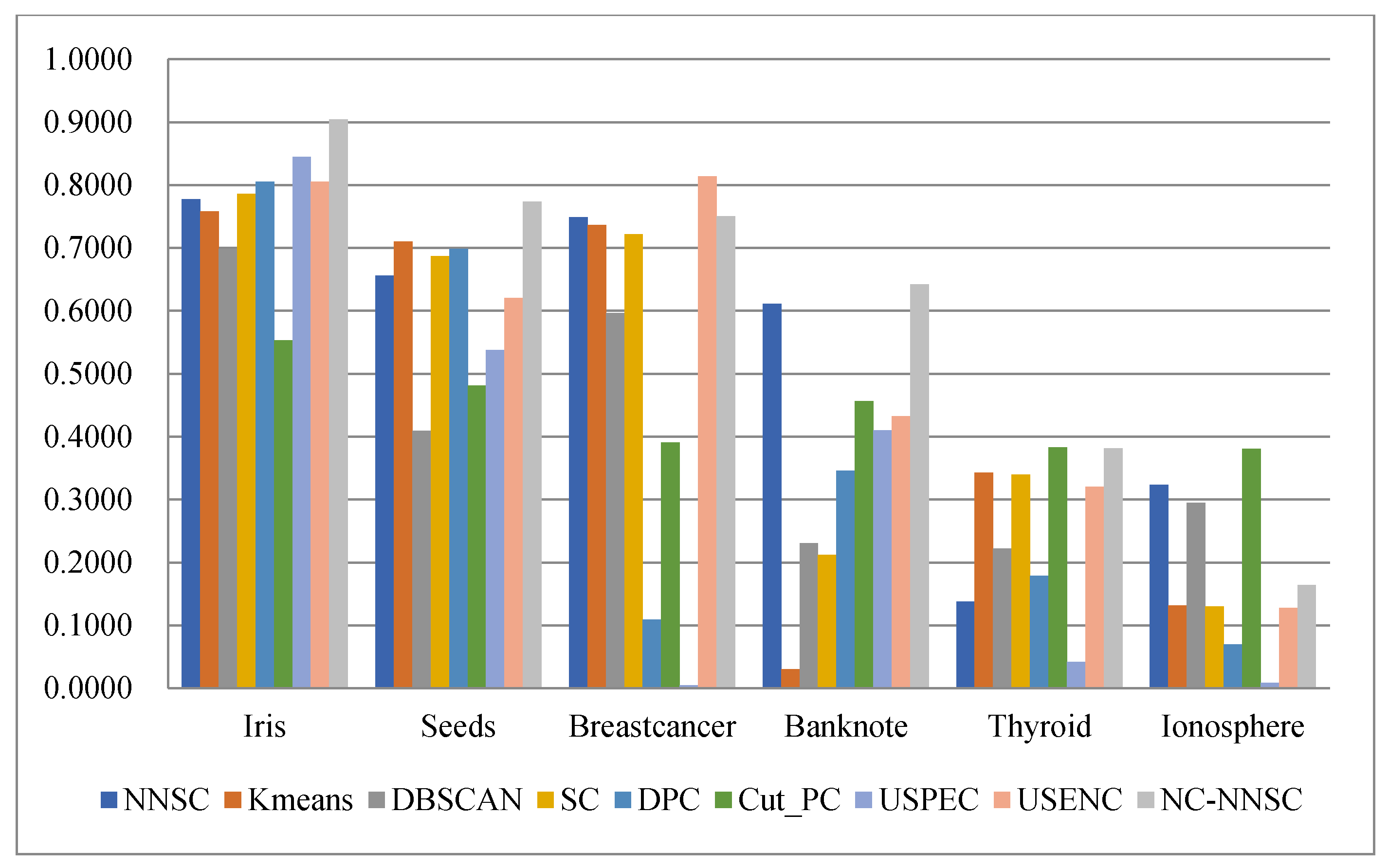
In order to more intuitively observe the Acc, ARI, F-measure, and NMI of the nine algorithms on the six real UCI data sets, histograms have been used to represent them, as shown in Figure 15, Figure 16, Figure 17 and Figure 18.

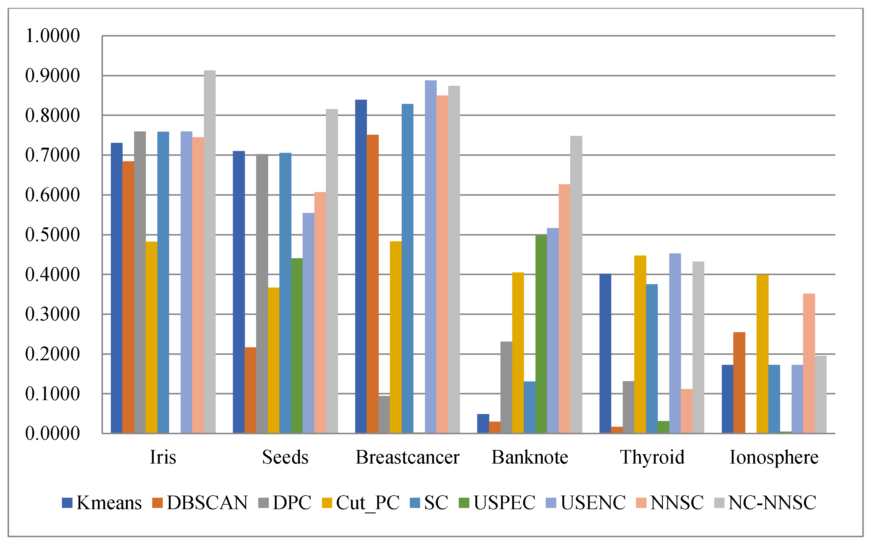
Regarding accuracy, as shown in Figure 15, except for the banknote data set, the NCNNSC-CP algorithm has the best results on the five UCI data sets. The result on the banknote dataset is also the second best. In terms of accuracy, Figure 16 demonstrates that although the proposed algorithm has general results on the two data sets of Thyroid and Ionosphere, it has achieved excellent results on the three data sets of Iris, Seeds, and Banknote. At the same time, it is second only to the USENC algorithm on the Breastcancer data set. As for F-measure, it is obvious that the NCNNSC-CP algorithm performs best on all data sets from Figure 17. In the aspect of the NMI, as displayed in Figure 18, except for the general performance on the ionosphere data set, the proposed algorithm achieved the best results on the three datasets of Iris, Seeds, and Banknote, and also achieved the second-best results on the datasets of Breastcancer and Thyroid.

Based on the above analysis, compared with other clustering algorithms, the NCNNSC-CP algorithm proposed in this paper has excellent performance in clustering.

4.5. Result Analysis

As aforementioned, combining the experimental results on the synthetic data set and the real data set, compared with other comparison algorithms, the Noises Cutting and Natural Neighbors Spectral Clustering Based on Coupling P System is better. For different types of clusters, the corresponding shapes can be correctly identified. Moreover, the difference in the size of each data set can indicate that the NCNNSC-CP method can obtain effective clustering results for data sets of different scales and can be applied to more complex situations. In this paper, all the procedures of the algorithm are carried out in the structure of the coupled P system. Taking advantage of the extremely parallel computing characteristics of the coupled P system in membrane computing, the computing efficiency is improved theoretically. In the part of noises recognition and cutting, all data points in the data set are determined in parallel at the same time, instead of the traditional sequential method. After the noise is identified, the noise points can be transported to the environment in real-time and discarded. When the processed data are clustered by the K-means algorithm, the c randomly selected cluster centers are simultaneously operated in parallel on the c sub-cells in the coupled P system. Membrane computing has the characteristics of extremely parallelism. In the constructed coupled P system, it can theoretically operate in parallel, which can improve efficiency to a certain extent.

5. Conclusions

In this paper, we propose noise cutting and natural neighbors spectral clustering based on coupled P system. The concept of natural neighbors and the method of spectral clustering are integrated into the coupled P system. The entire algorithm flow runs under the framework of the coupled P system, which detect and cut noises through the concepts of critical density and reverse density of natural neighbors. At the same time, the core natural neighbors of each data object are automatically determined from the noise-processed dataset, and the affinity matrix of spectral clustering is constructed according to the core natural neighbors. Then, further cluster them to achieve the final clustering result. Experimental results indicate that the proposed algorithm is better than other algorithms on artificially synthetic datasets and UCI real data sets.

In future work, we will further expand the CP system so that it can solve more optimization and clustering problems. Moreover, it will further improve the performance of the algorithm, such as the consideration of the automatic determination of the number of clusters, and the further improvement of the final clustering algorithm.

References

- Favati, P.; Lotti, G.; Menchi, O.; Romani, F. Construction of the similarity matrix for the spectral clustering method: Numeri-cal experiments. Comput. Appl. Math. 2020, 375, 112795. [Google Scholar] [CrossRef] [Green Version]
- Nataliani, Y.; Yang, M.-S. Powered Gaussian kernel spectral clustering. Neural Comput. Appl. 2017, 31, 557–572. [Google Scholar] [CrossRef]
- Huang, X.; Ye, Y.; Zhang, H. Extensions of Kmeans-Type Algorithms: A New Clustering Framework by Integrating Intra-cluster Compactness and Intercluster Separation. IEEE Trans. Neur. Net. Lear. 2014, 25, 1433–1446. [Google Scholar] [CrossRef]
- Martínez-Pérez, A. On the Properties of α-Unchaining Single Linkage Hierarchical Clustering. J. Classif. 2016, 33, 118–140. [Google Scholar] [CrossRef]
- Chen, Y.; Zhou, L.; Bouguila, N.; Wang, C.; Chen, Y.; Du, J. BLOCK-DBSCAN: Fast Clustering For Large Scale Data. Pattern Recognit. 2021, 109, 107624. [Google Scholar] [CrossRef]
- Jokinen, J.; Raty, T.; Lintonen, T. Clustering structure analysis in time-series data with density-based clusterability measure. IEEE/CAA J. Autom. Sin. 2019, 6, 1332–1343. [Google Scholar] [CrossRef]
- Kim, H.S.; Gao, S.; Xia, Y.; Kim, G.B.; Bae, H.Y. DGCL: An efficient density and grid based clustering algorithm for large 610 spatial database. In Proceedings of the 7th International Conference on Advances in Web-Age Information Management 611 (WAIM), Hong Kong, China, 17–19 June 2006; Volume 4016, pp. 362–371. [Google Scholar]
- Márquez, D.G.; Otero, A.; Félix, P.; García, C.A. A novel and simple strategy for evolving prototype based clustering. Pattern Recognit. 2018, 82, 16–30. [Google Scholar] [CrossRef]
- Yan, W.; Shi, S.; Pan, L.; Zhang, G.; Wang, L. Unsupervised change detection in SAR images based on frequency difference and a modified fuzzy c-means clustering. Int. J. Remote Sens. 2018, 39, 3055–3075. [Google Scholar] [CrossRef]
- Janani, R.; Vijayarani, S. Text document clustering using Spectral Clustering algorithm with Particle Swarm Optimization. Expert Syst. Appl. 2019, 134, 192–200. [Google Scholar] [CrossRef]
- Sun, P.; Gao, L.; Han, S. Identification of overlapping and non-overlapping community structure by fuzzy clustering in com-plex networks. Inform. Sciences 2011, 181, 1060–1071. [Google Scholar]
- Ge, C.; Oliveira, R.; Gu, I.; Bollen, M. Deep Feature Clustering for Seeking Patterns in Daily Harmonic Variations. IEEE Trans. Instrum. Meas. 2020, 70, 3016408. [Google Scholar] [CrossRef]
- Nascimento, M.; de Carvalho, A. Spectral methods for graph clustering—A survey. Eur. J. Oper. Res. 2011, 211, 221–231. [Google Scholar] [CrossRef]
- Chen, W.; Feng, G. Spectral clustering: A semi-supervised approach. Neurocomputing 2012, 77, 229–242. [Google Scholar] [CrossRef]
- Huang, D.; Wang, C.-D.; Wu, J.-S.; Lai, J.-H.; Kwoh, C.-K. Ultra-Scalable Spectral Clustering and Ensemble Clustering. IEEE Trans. Knowl. Data Eng. 2020, 32, 1212–1226. [Google Scholar] [CrossRef] [Green Version]
- Bian, Z.; Ishibuchi, H.; Wang, S. Joint Learning of Spectral Clustering Structure and Fuzzy Similarity Matrix of Data. IEEE Trans. Fuzzy Syst. 2019, 27, 31–44. [Google Scholar] [CrossRef]
- Li, X.-Y.; Guo, L.-J. Constructing affinity matrix in spectral clustering based on neighbor propagation. Neurocomputing 2012, 97, 125–130. [Google Scholar] [CrossRef]
- Ye, X.; Sakurai, T. Spectral clustering with adaptive similarity measure in Kernel space. Intell. Data Anal. 2018, 22, 751–765. [Google Scholar] [CrossRef]
- Wu, L.F.; Chen, P.Y.; Yen, E.H.; Xu, F.L.; Xia, Y.L.; Aggarwal, C. Scalable Spectral Clustering Using Random Binning Features. In Proceedings of the 24th ACM SIGKDD International Conference on Knowledge Discovery and Data Mining, London, UK, 9–23 August 2018; Guo, Y., Farooq, F., Eds.; Association for Computing Machinery: New York, NY, USA, 2018; pp. 2506–2515. [Google Scholar]
- Păun, G. Computing with Membranes. J. Comput. Syst. Sci. 2000, 61, 108–143. [Google Scholar] [CrossRef] [Green Version]
- Song, T.; Gong, F.; Liu, X.; Zhao, Y.; Zhang, X. Spiking Neural P Systems With White Hole Neurons. IEEE Trans. NanoBiosci. 2016, 15, 666–673. [Google Scholar] [CrossRef]
- Zhao, Y.; Liu, X.; Wang, W. Spiking Neural P Systems with Neuron Division and Dissolution. PLoS ONE 2016, 11, e0162882. [Google Scholar] [CrossRef]
- Zhang, G.-X.; Pan, L.-Q. A Survey of Membrane Computing as a New Branch of Natural Computing. Chin. J. Comput. 2010, 33, 208–214. [Google Scholar] [CrossRef]
- Wu, T.; Pan, L. The computation power of spiking neural P systems with polarizations adopting sequential mode induced by minimum spike number. Neurocomputing 2020, 401, 392–404. [Google Scholar] [CrossRef]
- Peng, H.; Li, B.; Wang, J.; Song, X.; Wang, T.; Valencia-Cabrera, L.; Pérez-Hurtado, I.; Riscos-Núñez, A.; Pérez-Jiménez, M.J. Spiking neural P systems with inhibitory rules. Knowl.-Based Syst. 2020, 188, 105064. [Google Scholar] [CrossRef]
- Rong, H.; Yi, K.; Zhang, G.; Dong, J.; Paul, P.; Huang, Z. Automatic Implementation of Fuzzy Reasoning Spiking Neural P Systems for Diagnosing Faults in Complex Power Systems. Complex 2019, 2019, 1–16. [Google Scholar] [CrossRef]
- Jiang, Z.; Liu, X. Novel coupled DP system for fuzzy C-means clustering and image segmentation. Appl. Intell. 2020, 50, 4378–4393. [Google Scholar] [CrossRef]
- Liu, X.; Xue, A. Communication P systems on simplicial complexes with applications in cluster analysis. Discret. Dyn. Nat. Soc. 2012, 2012, 415242. [Google Scholar] [CrossRef]
- Ng, A.Y.; Jordan, M.I.; Weiss, Y. On Spectral Clustering: Analysis and an Algorithm. Adv. Neural Inf. Process. Syst. 2001, 2, 849–856. [Google Scholar]
- Zhu, Q.; Feng, J.; Huang, J. Natural neighbor: A self-adaptive neighborhood method without parameter K. Pattern Recognit. Lett. 2016, 80, 30–36. [Google Scholar] [CrossRef]
- Huang, J.; Zhu, Q.; Yang, L.; Feng, J. A non-parameter outlier detection algorithm based on Natural Neighbor. Knowl.-Based Syst. 2016, 92, 71–77. [Google Scholar] [CrossRef]
- Jain, A.K. Data clustering: 50 years beyond K-means. Pattern Recognit. Lett. 2010, 31, 651–666. [Google Scholar] [CrossRef]
- Ester, M.; Kriegel, H.P.; Sander, J.; Xu, X. A Density-Based Algorithm for Discovering Clusters in Large Spatial Databases with Noise. In Proceedings of the 2nd International Conference on Knowledge Discovery and Data Mining KDD-96, Portland, OR, USA, 2–4 August 1996; pp. 226–231. [Google Scholar]
- Rodriguez, A.; Alessandro, L. Clustering by fast search and find of density peaks. Science 2014, 344, 1492–1496. [Google Scholar] [CrossRef] [PubMed] [Green Version]
- Li, L.-T.; Xiong, Z.-Y.; Dai, Q.-Z.; Zha, Y.-F.; Zhang, Y.-F.; Dan, J.-P. A novel graph-based clustering method using noise cutting. Inf. Syst. 2020, 91, 91. [Google Scholar] [CrossRef]
- Mohammed, J.; Wagner, M. Data Mining and Analysis: Fundamental Concepts and Algorithms; Cambridge University Press: Cambridge, UK, 2014; pp. 37–68. [Google Scholar]
Figure 1.
The basic membrane structure of the cell-like P system.
Figure 2.
The basic membrane structure of the tissue-like P system.
Figure 3.
The flow chart of the proposed NCNNSC-CP algorithm.
Figure 4.
The basic structure of the coupled P system.
Figure 5.
The original data of the nine synthetic data sets.
Figure 6.
The results of 9 clustering algorithms in D1.
Figure 7.
The results of 9 clustering algorithms in D2.
Figure 8.
The results of 9 clustering algorithms in D3.
Figure 9.
The results of 9 clustering algorithms in D4.
Figure 10.
The results of 9 clustering algorithms in D5.
Figure 11.
The results of 9 clustering algorithms in D6.
Figure 12.
The results of 9 clustering algorithms in D7.
Figure 13.
The results of 9 clustering algorithms in D8.
Figure 14.
The results of 9 clustering algorithms in D9.
Figure 15.
The Accuracy index of different clustering algorithms in six real-world datasets.
Figure 16.
The Adjusted Rand Index (ARI) index of different clustering algorithms in six real-world datasets.
Figure 17.
The F-measure index of different clustering algorithms in six real-world datasets.
Figure 18.
The NMI index of different clustering algorithms in six real-world datasets.