
Dynamic and Statistical Operability of an Experimental Batch Process


1
Graduate Program of Chemical Engineering, Federal University of Campina Grande, Aprigio Veloso St. 882, Campina Grande 58428-830, Brazil
2
Department of Chemical and Biomedical Engineering, West Virginia University, Morgantown, WV 26506, USA
*
Author to whom correspondence should be addressed.
Processes 2021, 9(3), 441; https://0-doi-org.brum.beds.ac.uk/10.3390/pr9030441
Submission received: 31 December 2020
/
Revised: 19 February 2021
/
Accepted: 22 February 2021
/
Published: 28 February 2021
(This article belongs to the Special Issue Redesign Processes in the Age of the Fourth Industrial Revolution)
Abstract
:The operability approach has been traditionally applied to measure the ability of a continuous process to achieve desired specifications, given physical or design restrictions and considering expected disturbances at steady state. This paper introduces a novel dynamic operability analysis for batch processes based on classical operability concepts. In this analysis, all sets and statistical region delimitations are quantified using mathematical operations involving polytopes at every time step. A statistical operability analysis centered on multivariate correlations is employed for the first time to evaluate desired output sets during transition that serve as references to be followed to achieve the final process specifications. A dynamic design space for a batch process is, thus, generated through this analysis process and can be used in practice to guide process operation. A probabilistic expected disturbance set is also introduced, whereby the disturbances are described by pseudorandom variables and disturbance scenarios other than worst-case scenarios are considered, as is done in traditional operability methods. A case study corresponding to a pilot batch unit is used to illustrate the developed methods and to build a process digital twin to generate large datasets by running an automated digital experimentation strategy. As the primary data source of the analysis is built in a time-series database, the developed framework can be fully integrated into a plant information management system (PIMS) and an Industry 4.0 infrastructure.
1. Introduction
The concepts of process operability defined by Vinson and Georgakis [1] have been widely studied and applied to several linear and non-linear systems. In essence, process operability allows the analysis of the achievable output set (AOS) that a process can reach, considering an available input set (AIS) and an expected disturbance set (EDS), for a given process model. This analysis can also verify if the desired output set (DOS) can be achieved and quantify how much of the AOS covers the DOS specifications by defining an operability index (OI) [2]. The inputs for the analysis correspond to the process design and operational limitations, environmental constraints, as well as a group of external disturbances. The outputs cover production targets, quality specifications, business benchmarks, and safety-critical conditions [3].
Past operability studies have also considered the application of operability to control strategies [4,5], process intensification [6,7], and design optimization [8,9]. The operability framework has been extensively studied from a steady-state point of view [10], in which the graphical regions used consisted of mainly stable points of operation [11,12]. Other studies have investigated the dynamic operability concerning the minimum time to achieve different steady states [13,14]. Additionally, these previously reported studies have considered only deterministic sets, without statistical or probabilistic concepts being involved.
In this work, a dynamic operability study is conducted based on classical operability concepts [11,15]. The operability analysis previously developed for steady-state conditions is performed for each time step as the process evolves, and thus the sets and OI values are indexed by timestamp. In classical operability studies, the EDS is defined by the disturbance values representing worst-case scenarios [16]. However, for a process where the disturbances follow a statistical distribution, these scenarios have only a small probability of occurring. In this proposed method, the EDS is considered from a probabilistic standpoint, whereby Gaussian (±3σ) distributions are defined for a disturbance and the disturbance values are generated from random selections. Statistical concepts are also used to build the DOS sets by taking the correlations between variables into account. This idea has been previously employed for multivariate statistical quality control (SQC) using the variance–covariance matrix [17] as a reference to draw the joint reliability region [18,19]. As only data are needed to build these sets, intermediate DOS probabilistic regions can be generated along with the process dynamic operation instead of only a deterministic DOS, as in the classical operability approach.
The case study chosen to apply the proposed dynamic operability approach is a batch reactor due to the associated challenges with this mode of operation—a batch process is intrinsically dynamic, i.e., the operating conditions are time-varying [20]. According to industrial practice, there are always ranges for product specifications, and once the product lies within the desired range, the batch is considered finished and the product is acceptable [21]. However, these requirements are only specified at the end of the batch. As a major contribution of this work, a space trajectory is provided to serve as a path to be followed to reach these final specifications.
For the batch application system, a design of experiments (DoE) approach is performed to guide the operations of a pilot plant unit, as well as the development and simulation of a digital twin for the plant. The term digital twin has earned popularity during the so-called “fourth industrial revolution”, indicating in this context a high-fidelity model that can represent a real process, and thus can be extrapolated or interpolated to different process conditions. This process digital twin is created in Aspen Batch Modeler (ABM from AspenTech) and can be automatically called by a VBA code via Aspen Simulation Workbook in order to connect with the operability algorithms developed in MATLAB. The developed framework is, thus, ready for incorporation into so-called “Industry 4.0” infrastructure, where massive amounts of data can be generated and updated in real time by systems such as a plant information management system (PIMS).
Therefore, this work aims to contribute to the following aspects of process operability: (i) tackles operability w.r.t. a dynamic point of view by evaluating classical operability concepts over time and their applicability to batch processes; (ii) incorporates statistical concepts into the expected disturbance and desired output set definitions.
This paper is structured as follows. First, the classical process operability concepts are reviewed in Section 2 and the definitions of the proposed approach (dynamic and statistical operability) are introduced in Section 3. Then, the case study is presented along with the dynamic operability application in Section 4. Additionally, in Section 4 the automated digital experimentation technique is detailed, while in Section 5 the main algorithm is described. The results from the digital twin validation process and the proposed method are discussed in Section 6, with conclusions given in Section 7.
2. Classical Process Operability Concepts
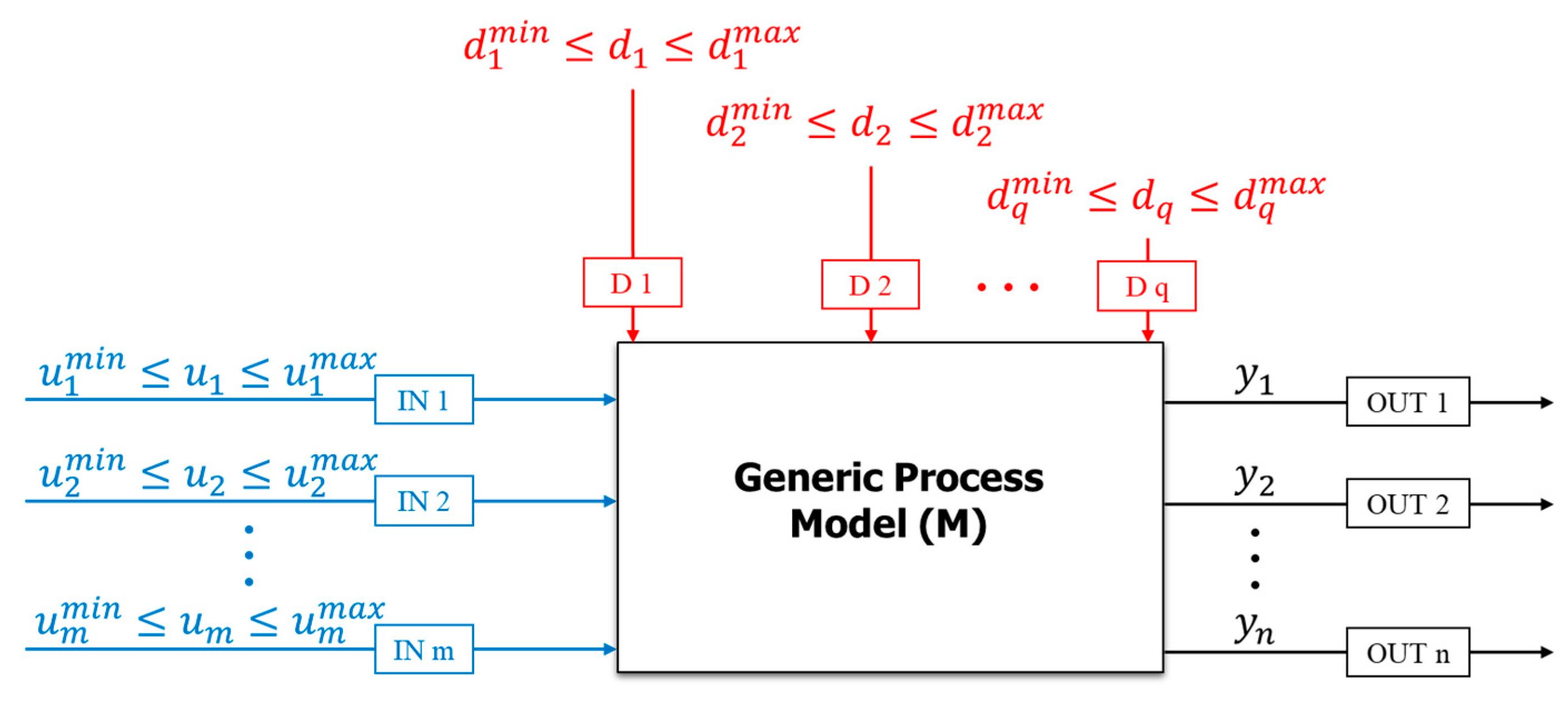
Operability concepts enable the understanding of how a process can reach desired specifications when subjected to input conditions and limited by design constraints, while considering expected disturbances. In the process operability framework, a generic process model is defined as shown in Figure 1, in which inputs, , are manipulated inside their available limits, and along with disturbances, , stimulate the model (M) to generate the outputs, [3,15].
The process model (M) can be defined by the first principles or process simulators (e.g., in Aspen Plus, DYNSIM, AVEVA Process Simulation, etc.) to reproduce a real unit and obtain the relationships between input and output spaces [3]. The following sets are essential for the operability analysis:
- Available input set (AIS)—Considers all available inputs that may change within a specific range according to physical or operating constraints. This set may represent design or operational inputs. Operational inputs are manipulated variables (MV) subject to control studies, whereas design inputs can be related to process materials, design dimensions, etc. [11,16]. This set is defined as:
- Expected disturbance set (EDS)—Represents the known process uncertainties, usually chosen as the extreme values in order to consider worst-case scenarios [16].
- Achievable output set (AOS)—Compiles all possible outputs that the system can achieve, given the AIS and considering an EDS. Thus, this set is defined as a function of inputs and disturbances. For each disturbance scenario, , the AOS can be obtained as [12]:The intersection of all AOS(d)s yields the AOS (shown in Equation (4)), which is a region where the setpoints of the output variables can be moved successfully using the available control action in the AIS while compensating for any disturbances in the EDS [12].
- Desired output set (DOS)—Corresponds to the desired region to be obtained for the process. This set may be defined, for example, by production requirements such as production rates or product qualities, process specifications, or efficiency. The DOS is mathematically defined in Equation (5) [11].
The DOS can be described by straight edges that connect the vertices given by and for each output or discontinuous or disjointed points that discretize such edges [3]. In practice, a process is fully operable if all outputs satisfy the desired requirements, i.e., the DOS is a subset of the AOS. The operability index (OI) is defined to quantify the achievability of the DOS, as shown in Equation (6). If some regions of the DOS are not achievable, the OI is, thus, less than one [12].
where represents a measure of the size of the set, e.g., area for 2-D sets, hypervolume for high-D sets, etc. Thus, mathematical operations involving intersections of polytopes, such as AOS ∩ DOS, need to be performed to determine the OI. For such operations, the Multi-Parametric Toolbox (MPT) [22] in MATLAB can be used for convex regions. For non-convex regions, the MATLAB built-in subroutine “boundary” may be employed.
In the classical operability methods, these sets are mainly studied at steady-state conditions. The existing dynamic approach investigates the operability from the standpoint of the minimum time required for a system to move between steady states and reject expected disturbances. Existing dynamic operability methods can also be used to calculate the amount of constraint relaxation necessary to prevent the occurrence of transient infeasibilities when disturbances affect the process [13,16]. The analysis proposed in the next section considers the extension of the existing operability methods for the calculation of dynamic sets employing concepts of statistics.
3. Proposed Approach: Dynamic and Statistical Operability
The classical steady-state operability concepts have inspired the proposed method introduced in this section, which now considers the entire time frame, including the process transient operations. In particular, the AIS remains the same as the concept described by Equation (1), with the values indexed at the initial time (). The other sets have to be redefined, considering their categorization in terms of their variable abilities to be manipulated during process operation. For example, a reactant concentration can be manipulated at the beginning of the batch, however once the reaction occurs, it will be dependent on the process design and mass and energy balances. However, the amount of fluid entering the jacket is always changeable. Therefore, two categories may be defined for the process variables:
- Static—no handling is available during the process and it is typically defined at the beginning, e.g., for the initial temperature and concentrations;
- Dynamic—the values can be changed during operation, whether in an open or closed loop, e.g., for the thermal fluid inlet flow and temperature.
3.1. Expected Disturbance Set
The new EDS definition considers a probabilistic approach, in which not only are the worst-case scenarios analyzed, but also the intermediate ones with more likelihood of occurring. The dynamic and probabilistic expected disturbance set (EDSp(t)) is defined by Equation (7) as follows:
- Disturbance intensity—The deviation from the nominal value of the disturbance variable is assumed random for unbiased processes and with a Gaussian behavior. Essentially, this work considers ±3σ limits for and as in Equation (7) and the generation of random disturbances within these bounds;
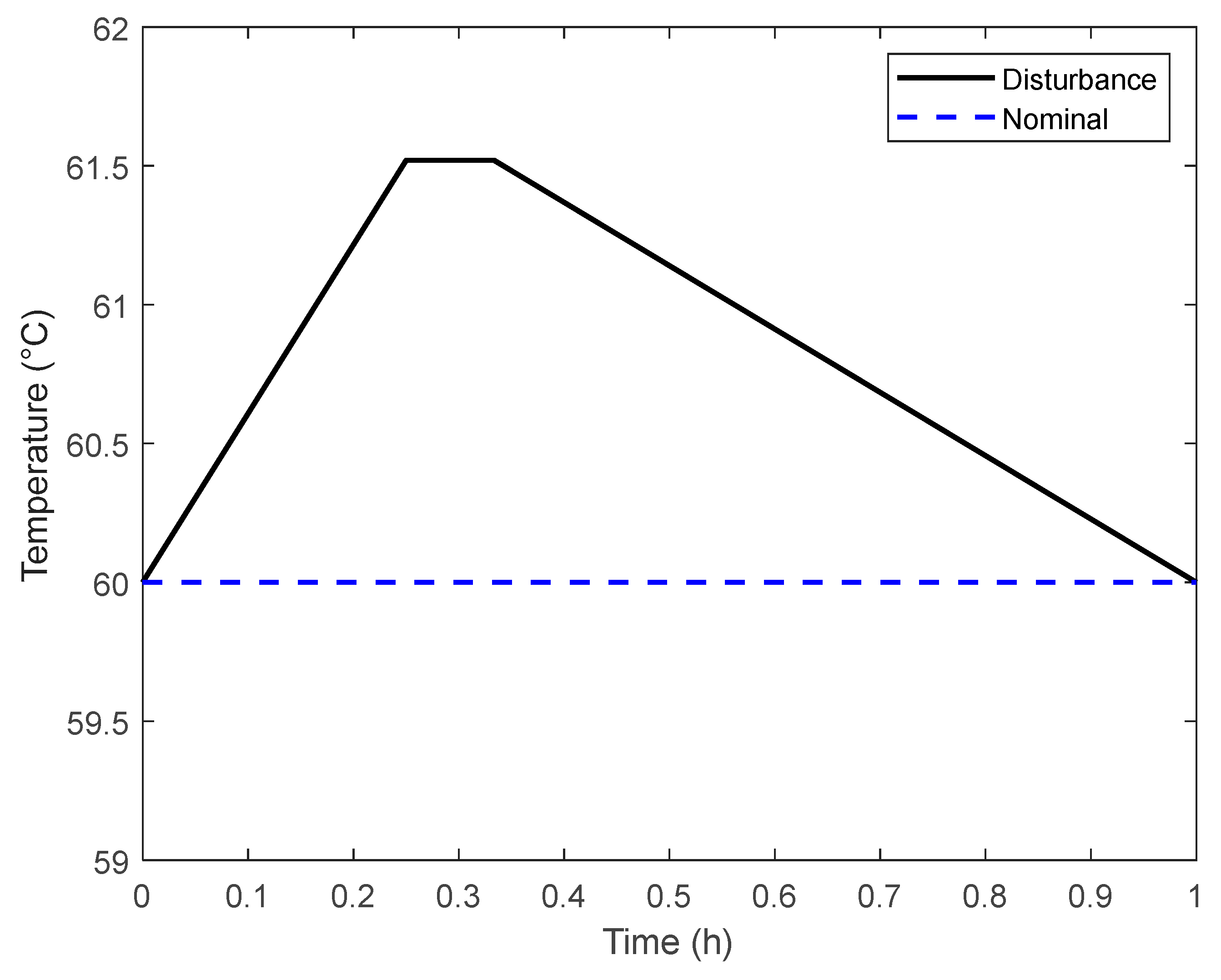
- Dynamic expectation—A disturbance may occur at any moment during operations, reaching a maximum value and then reducing its magnitude due to a control action; thus, it can have different behaviors (e.g., step or impulse). In this work, it is assumed that the disturbance follows a ramp, reaching the maximum value at 25%, 50%, or 75% for a one-hour long batch. Such disturbance intensity then remains for 5, 15, or 30 min, respectively. Figure 2 illustrates a disturbance example in which the temperature is affected, reaching 61.52 °C at the 15 min mark, remaining for 5 min, and then returning to its nominal value of 60.00 °C.
The more disturbance possibilities that are considered, the more representative the EDSp(t) is. In real batch reaction systems, historical data can be investigated to further characterize the disturbance behavior throughout the operation. In a PIMS infrastructure, time-series data for different variables, including disturbances, may come from sensors, estimators, or historical databases.
3.2. Achievable Output Set
As the outputs are considered time-dependent, AOS(d,t) defined by Equation (8) is indexed per timestamp and by the disturbance d, which is part of the EDSp(t).
The AOS(t) is similarly calculated as in the original definition, based on the intersection of the AOS(d,t)s for a specific time t given by Equation (9).
3.3. Desired Output Set
Previous operability studies shows the desired output set (DOS) as a set desired to be achieved at steady state [3,9]. For intrinsic time-dependent batch processes, the interest lies in the final process specification. Thus, the DOS() can be defined, where denotes the final time for the same definition as in Equation (5).
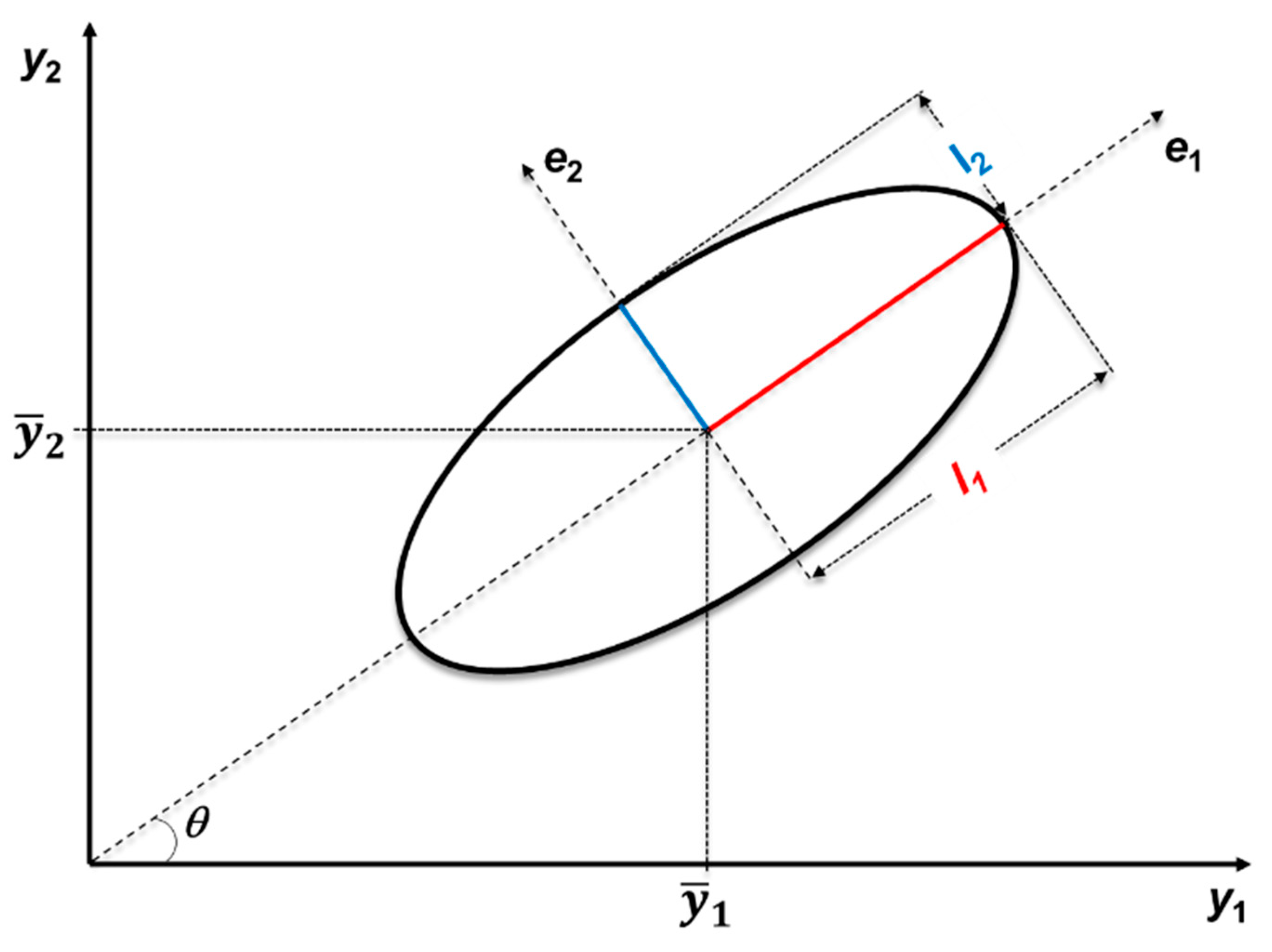
The proposed dynamic operability framework has to first consider the conditions capable of satisfying the DOS(). Based on these conditions, the dynamic profiles can be mapped backwards and the desired output set can be evaluated per timestamp, defining the DOS(t). This mapping strategy is based on a joint reliability region, which carries information about all variables/dimensions of DOS() and their self-correlations based on the covariance matrix. The proposed method, thus, relies on multivariate distributions that change their shape according to the variable interactions. Figure 3 is based on the concepts presented in [18,23] and shows an example from a bidimensional analysis of the desired regions represented by an ellipse.
For the ellipse in Figure 3, a perfect circle will be found if there is no correlation between and , while the ellipse becomes “thinner” as the relationship between variables strengthens. This shape change in Figure 3 is due to the eigenvalues () present in the semi-axis expression, which can be evaluated by Equation (10).
in which is the critical value of a chi-square distribution with degrees of freedom and level of significance. Additionally, the shape geometry is centered around the mean value () and has directions defined by the eigenvectors ( and ) and the angle . The ellipse parametric coordinates are described by Equations (11) and (12).
These multivariate concepts are the basis of the DOSp(t) definition. The DOSp(t), thus, represents the desired output region at a specific time t, in which the “p” subscript is due to its probabilistic nature. Therefore, the DOSp(t) can be mathematically defined as in Equation (13).
where n is the DOS dimension; thus, when n = 2, Equation (13) corresponds to an ellipse, n = 3 is an ellipsoid, and so on.
Finally, the dynamic operability index (OI(t)) is evaluated at each timestamp according to Equation (14). The lower the OI(t), the more attention is needed in the specific analyzed time period to guarantee the desired process specification. If no process condition can satisfy the DOS(), the OI() is null, resulting in batch run conditions that are not able to achieve the desired specifications.
4. Case Study Definition and Setup
This section presents a case study that consists of a pilot batch reactor system. The proposed operability script for this system is described along with the time-series dataset used. Additionally, the developed dynamic model for this system is validated against the pilot bench unit, producing a digital twin for the process. Following the script, automatic model runs are performed considering all of the recipes within a digital experimentation strategy encompassing 900 simulated conditions (with approximately 1000 generated points per simulated condition), which are defined based on the AIS and the EDSp(t).
4.1. Pilot Batch Unit
The addressed system is characterized by an endothermic second-order reaction between sodium hydroxide (NaOH) and ethyl acetate (), as described in Equation (15). This reaction is carried out in a 1.2L stirred batch reactor and follows the kinetic parameters according to [24]. In this reactor system, water flows in a jacket to transfer enough heat for isothermal operation. A pH indicator is used to mark the end of the reaction process. The experimental apparatus is depicted in Figure 4, where a thermocouple and an electrical conductivity meter are used to acquire the reactor’s temperature and concentration, respectively.
The heating fluid flows in a closed circuit, where electrical resistance is manipulated to control the reactor temperature. A peristaltic pump guarantees its setpoint flow, which is seated in a supervisory control and data acquisition (SCADA) system present in the vendor software and used in the pilot unit operation. The system is also able to acquire the data as a time-series database per batch. The reactants have been previously prepared at determined concentrations and volumes per experiment. The conversion is calculated based on the conductivity measurements, and along with temperature, represents the most relevant variables in the study.
The digital experimentation strategy is delimited by a sensitivity analysis involving different ethyl acetate concentrations (0.1, 0.05, and 0.07 mol/dm3) and temperatures (30, 35, and 40 °C), with a fixed sodium hydroxide concentration of 0.1 mol/dm3. The experimental pilot plant was used to develop and validate a process digital twin, enabling automated and extensive digital manipulation of the system with minimal financial cost and safety risks.
4.2. Dynamic Operability Sets Applied to the Batch Case Study
The categorization of the process variables employed is detailed in Table 1, and was used to define the available input set (AIS), as well as the probabilistic expected disturbance set (EDSp(t)). This categorization is essential when studying the AIS and EDS.
The considered AIS has four dimensions, as given in Equation (16), with three static variables, i.e., ones that can only be defined at the beginning of the batch. In particular, the two reactant solutions were previously prepared at specified concentrations. Additionally, the initial reactor temperature depends on the environmental conditions and the heating system capacity.
Equation (17) describes the EDSp. Unlike , the two static disturbances ( and ) only need an intensity to be defined in the beginning of the batch, with no duration. A ramp behavior is assumed for the dynamic disturbance to add complexity and simulate the real case, in which the disturbance first changes from its nominal value and varies to a maximum, where it remains for a certain period until a control system brings it back to its nominal value. The specifically considered disturbance values are detailed in Table A1 in the Appendix A.
The DOS() is defined by Equation (18), where and correspond to reactor conversion of sodium hydroxide and temperature, respectively. This definition is similar to Equation (5), but related to the batch end time. The batches that satisfy the DOS()—also known as the deterministic desired output set in this work—will serve as basis to calculate the intermediate DOSp(t)s, i.e., the probabilistic DOS’s.
4.3. Automated Digital Experimentation
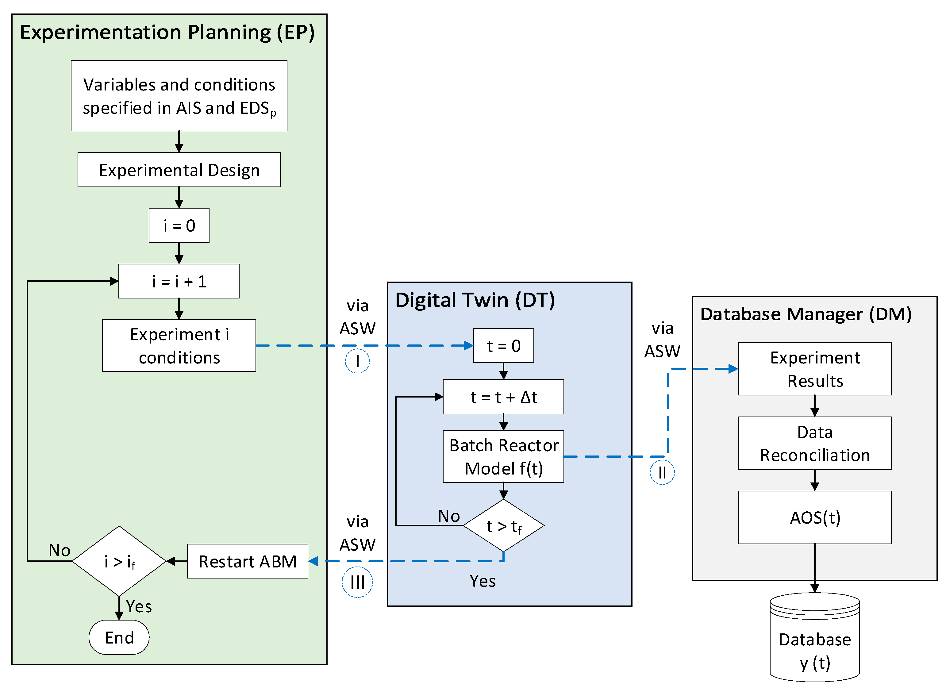
Due to the large number of experiments to be performed, an automated digital experimentation strategy is proposed using the Aspen software capability to communicate with Excel and Visual Basic for Applications (VBA) via Aspen Simulation Workbook (ASW). The batch recipes are defined by a multivariable experimental design formed by combinations of AIS and EDSp(t), with variables and conditions tabulated in a database. The strategy logics and queue organization are described in the experimentation planning (EP) module in Figure 5, in which a VBA code is written to assemble the recipe specifications and pass them to the process digital twin (DT) via ASW (Figure 5—step I).
The DT corresponds to an Aspen (ABM) model that provides the results at different timestamps because the AspenTech internal numerical method adjusts the time steps per batch to provide better convergence; hence, the data need to be reconciled before being archived in the final dataset. For this study, around 100 points for 10 variables are stored per one-hour batch. The outputs are sent to the database manager (DM) via ASW (Figure 5—step II). The DM is another VBA script responsible for writing the simulation outputs that converge in a time-series database. Not necessarily all runs will converge, since the EDSp(t) is pseudo-randomly generated; thus, a condition with no physical solution could be found, which would be reported with a trial status. Once the batch reaches the end, a signal is sent to EP via ASW (Figure 5—step III), and then the ABM is reset to start the next simulation. This loop detailed in Figure 5 is repeated until the last experiment is performed. The complete automated digital experimentation process produces approximately 900,000 data points.
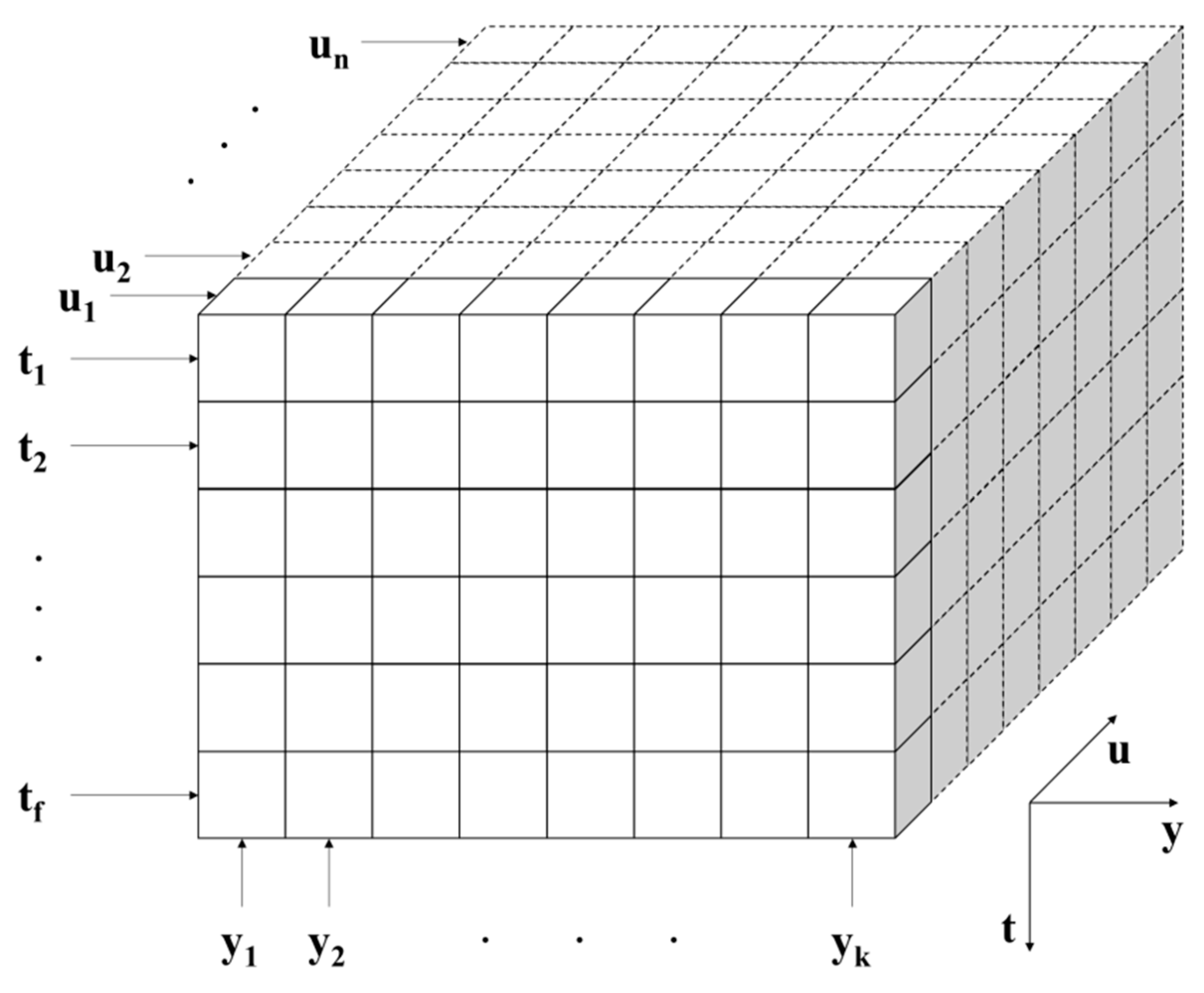
The MATLAB code (described in the next section) and VBA dynamic arrays organize the data in a tridimensional way according to Figure 6, where k response variables along time to have the information for the n batches. In such a way, all developed scripts can be expanded to more extensive cases as necessary.
5. Dynamic Operability Algorithm
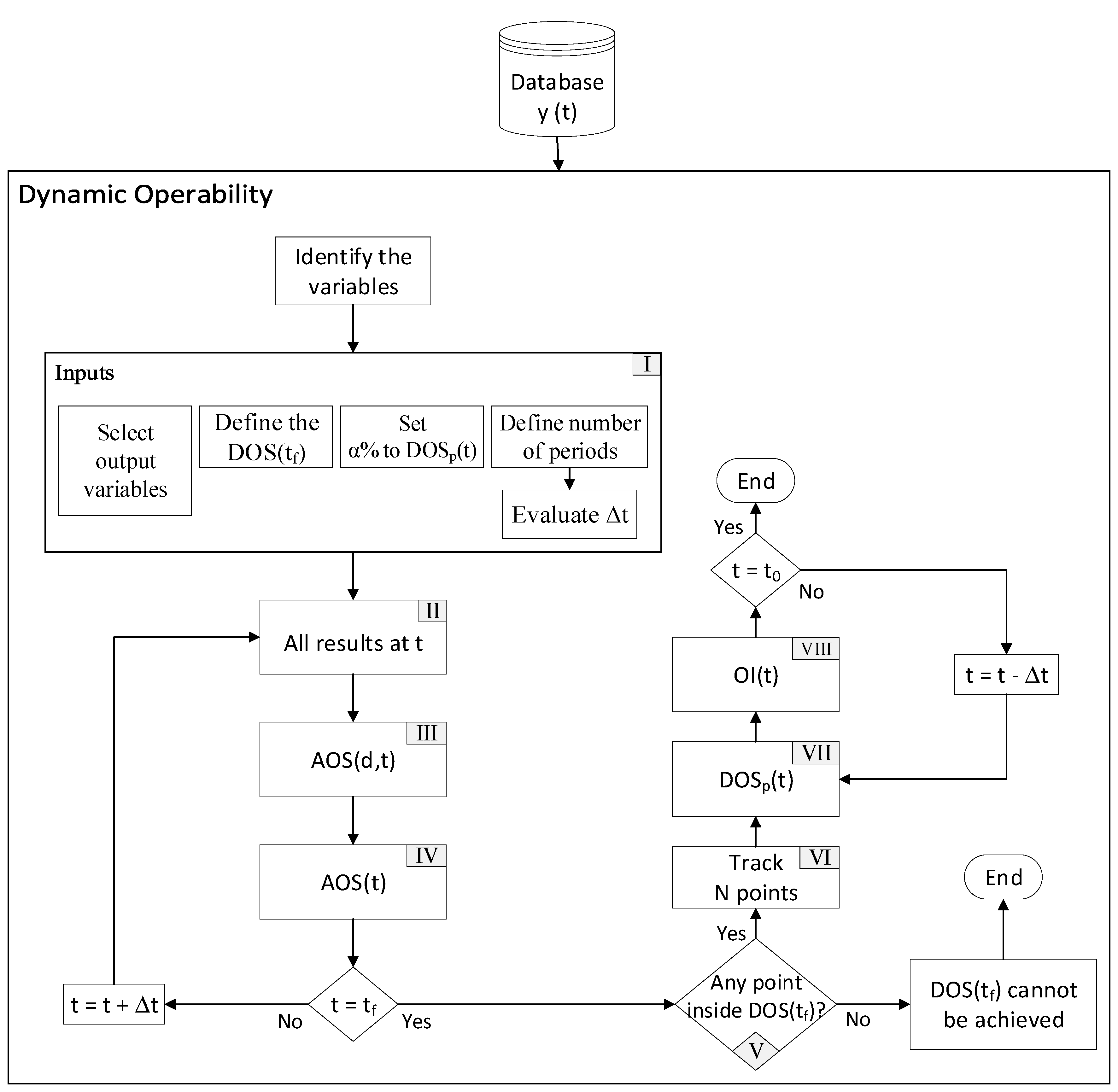
The dynamic operability analysis is implemented in MATLAB, according to the diagram described in Figure 7. Essentially, the time-series database is loaded first, the variables are identified, and after a few inputs to the algorithm have been defined, the methodology evaluation is started. These inputs correspond to:
- Output variables for AOS and DOS;
- DOS at the end of the batch (DOS());
- Tolerance allowed (α%) for the joint reliability regions of DOSp(t);
- Number of periods used during the process to run the analysis.
Once the dataset is loaded and inputs are defined (Figure 7—step I), all the results impacted by the first disturbance considered are combined (Figure 7—step II) at the beginning of the process (). Then, the AOS() is determined (Figure 7—step III) by a MATLAB built-in code called boundary. The Multi-Parametric Toolbox (MPT) was also tested for this calculation, but the boundary function demonstrated improved behavior in both convex and non-convex regions. Then, the AOS() is evaluated (Figure 7—step IV) using Equation (9). This procedure is repeated for all predefined periods until the final time (). Subsequently, the DOS() specifications described in Equation (18) are examined (Figure 7—step V). If no output satisfies these limits, the final requirements cannot be achieved by the process under the AIS conditions and considering the disturbances in the EDSp(t). Otherwise, the batches that fulfill the desired set are tracked (Figure 7—step VI) and the DOSp() is calculated (Figure 7—step VII) via the implementation of Equation (13). Finally, the areas of each AOS(t) and DOSp(t) are determined and the OI(t) is evaluated (Figure 7—step VIII). The last steps (Figure 7—VII and VIII) are repeated backward until the first timestamp is achieved.
6. Results
Initially, the validation of the digital twin model with the experimental results from the pilot plant is presented. Then, the dynamic operability results are shown for different sets, namely AOS(d,t), DOS(), and DOSp(t), as well as the OI(t) calculations.
6.1. Batch Model Validation with Experimental Results
The batch reactor temperature and sodium hydroxide molar concentration are used as variables for the model validation. The experiments are conducted until the acid–base indicator (crystal violet) marks the end of the reaction, with the same experiment duration applied as for the simulation.
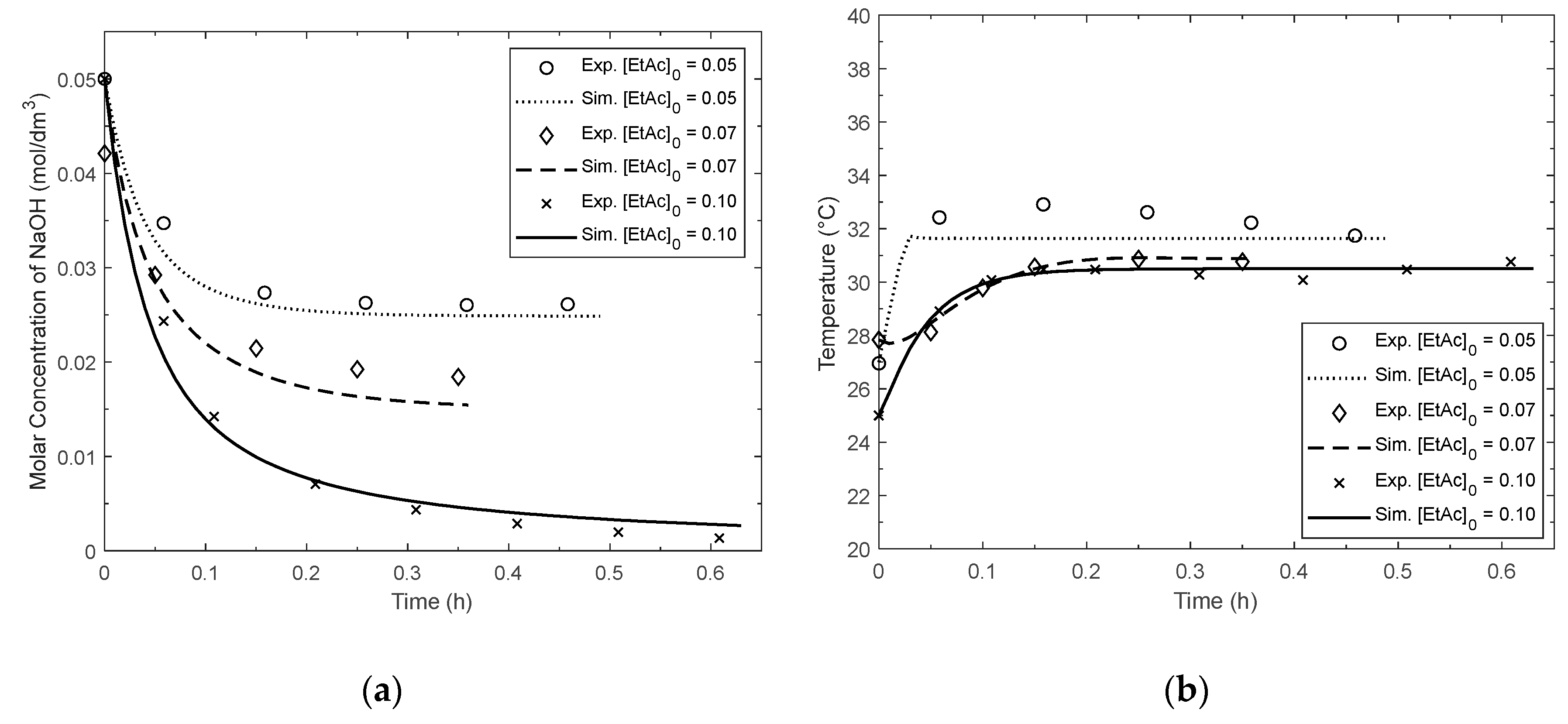
The comparisons between the pilot unit data and the simulated digital twin outcomes are presented for the experiments in Figure 8 and Figure 9. The sodium hydroxide concentration and reactor temperature profiles are shown in Figure 8a,b respectively for the fixed initial concentration of ethyl acetate specified in the legend.
The digital twin result profiles in Figure 8 thus closely represent the experimental ones for the entire batch. Specifically, the higher the initial concentration of ethyl acetate (EtAc), the more sodium hydroxide is converted; hence, the sodium hydroxide molar concentration is lowest when ethyl acetate starts at 0.10 mol/L. The highest relative error (4.0% approximately) occurs at the temperature profile for the lowest ethyl acetate initial concentration (0.05 mol/dm3); however, this condition did not substantially affect the molar concentration of sodium hydroxide over time.
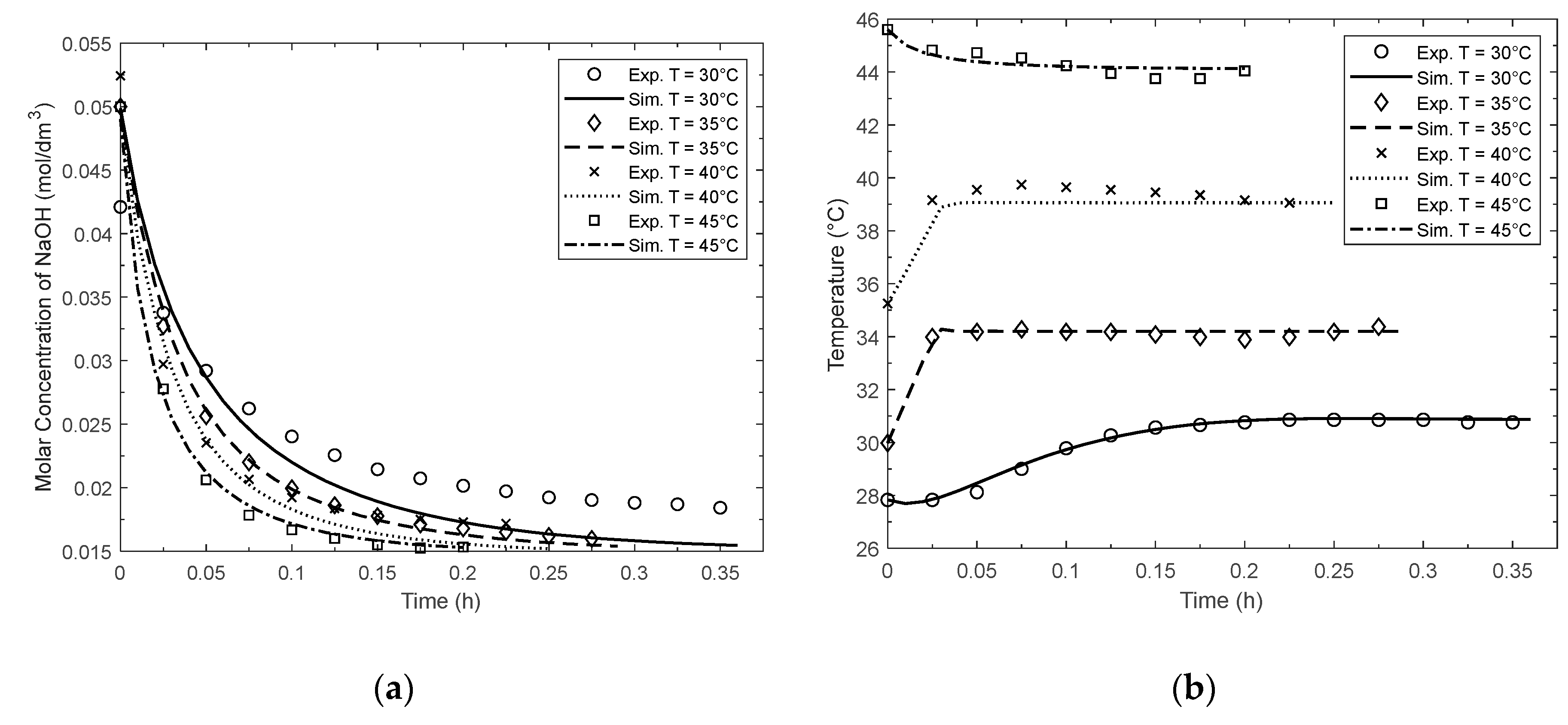
Figure 8 and Figure 9 indicate that the model matches the behavior shown by the experimental results of the pilot unit for all the sensitivity analyses performed for both concentration and temperature profiles. The highest relative error obtained was around 15% when the molar concentration was below 0.02 and the temperature was at 30 °C (see Figure 9), which is likely related to sensor precision. Thus, as the digital twin (DT) parameters are well adjusted to represent the entire batch system, this DT is used in the proposed dynamic and statistical operability approach. This ABM model is then simulated multiple times considering the cases determined by the design experimentation (see summary in Table A1). In this work, nearly a million data points were generated by the DT, with the corresponding data stored in a process database.
6.2. Dynamic and Statistical Operability Results
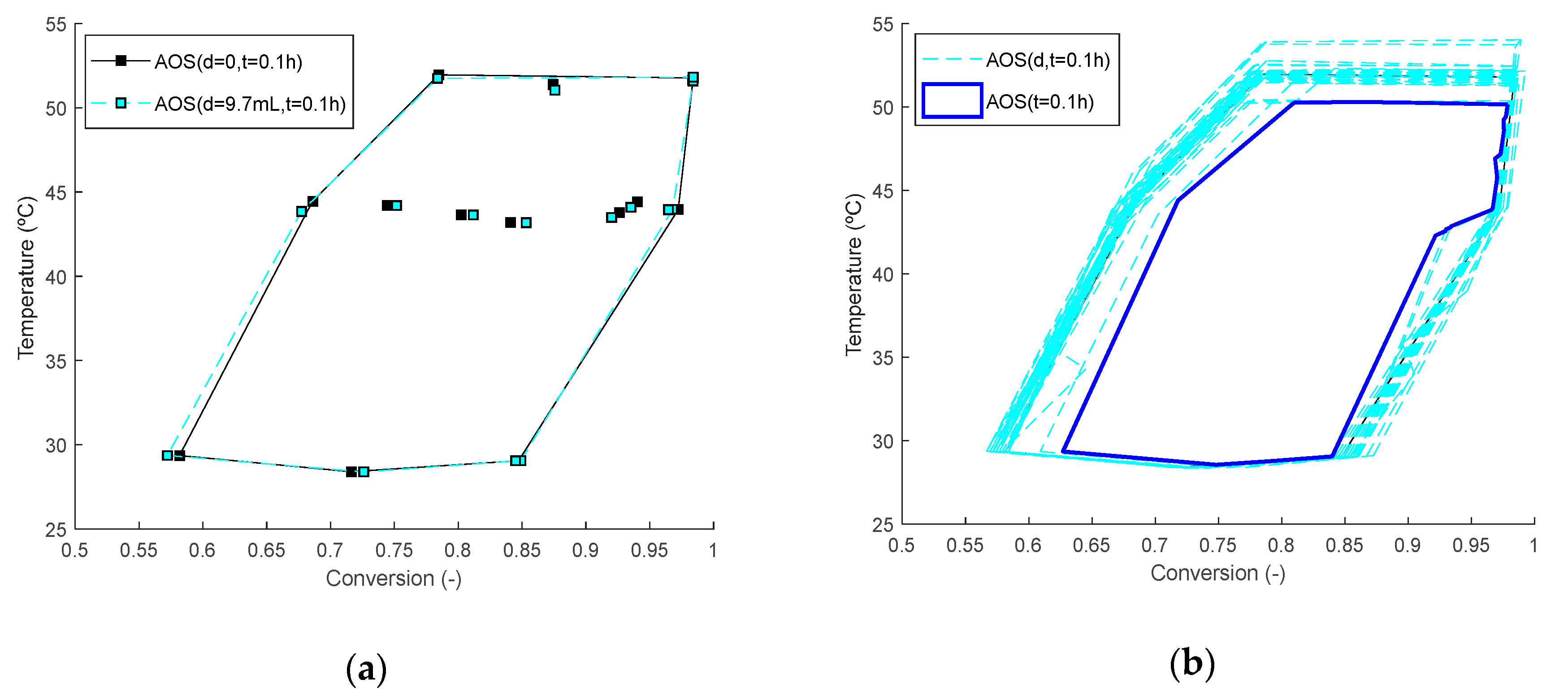
As at t = 0 h, there is no change in the system; the first AOS(d,t) is analyzed at t = 0.1 h, as depicted in Figure 10. In this figure, all of the outputs from the simulations at this timestamp are represented by the markers, while the non-disturbance case, i.e., AOS (d = 0, t = 0.1 h), is represented by the solid black line. The results from the non-disturbance case are plotted along with the ones obtained by the #1 disturbance case from Table A1—generating the AOS (d = 9.7, t = 0.1 h)—in Figure 10a.
Then, the outputs, AOS(d, t = 0.1 h), considering all the disturbance instances (in Table A1) are outlined by the dashed lines (light blue) in Figure 10b. Finally, the AOS(t = 0.1 h) is delimited by the solid line (dark blue) in Figure 10b, where the AOS(t = 0.1 h) is the intersection of all AOS(d,t = 0.1 h)s at 0.1 h and is the one used for operability index (OI) calculation purposes. For this figure, each region was outlined using the MATLAB boundary function, while mathematical operations such as intersections were determined using another built-in MATLAB function called “polybool”.
The procedure above is used to determine the AOS(d,t)s presented in Figure 11a with the output points and AOS(t)s in Figure 11b, at all ten timestamps considered during the batch operation. The developed script can consider as many intervals as are available in the data; however, for visualization purposes, the analysis here is delimited to 10 time instants.
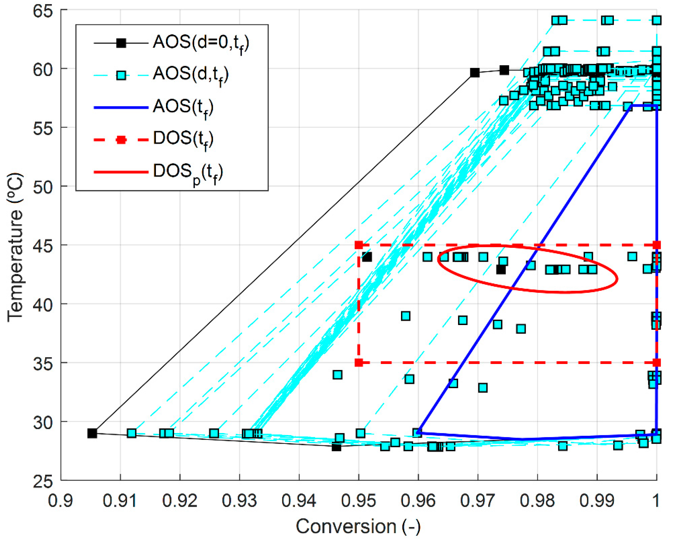
The plot of the deterministic desired output set (DOS()) at the end of the batch analyzes whether the designed process can achieve the specifications even with the expected disturbances. By deterministic, it is referred here to the set described by Equation (18), outlined by lower and upper limits and considering no statistical interaction among variables. The output points that satisfy the deterministic DOS() are indexed and used to build the primary joint reliability region at the final timestamp, i.e., DOSp(), as shown in Figure 12.
The DOSp() is, thus, the tolerance region considered for control purposes, with its center pulled by the region with the highest concentration of data, as shown by the ellipse in Figure 12. Additionally, the DOSp() is outlined by considering the tolerance at 60%. The data in Figure 12 are highly concentrated (with many points overlapping each other) at 98–100% conversion and 58–65 °C, as well as at 35–45 °C and 95–100% conversion, which is the set used to build the DOSp(). Thus, if the desired output set is centered in a range different from these conditions (such as around 47–56 °C and 95–100%), the desired specifications might not be achieved after a 1 h batch with the AIS and EDSp(t) described in this work.
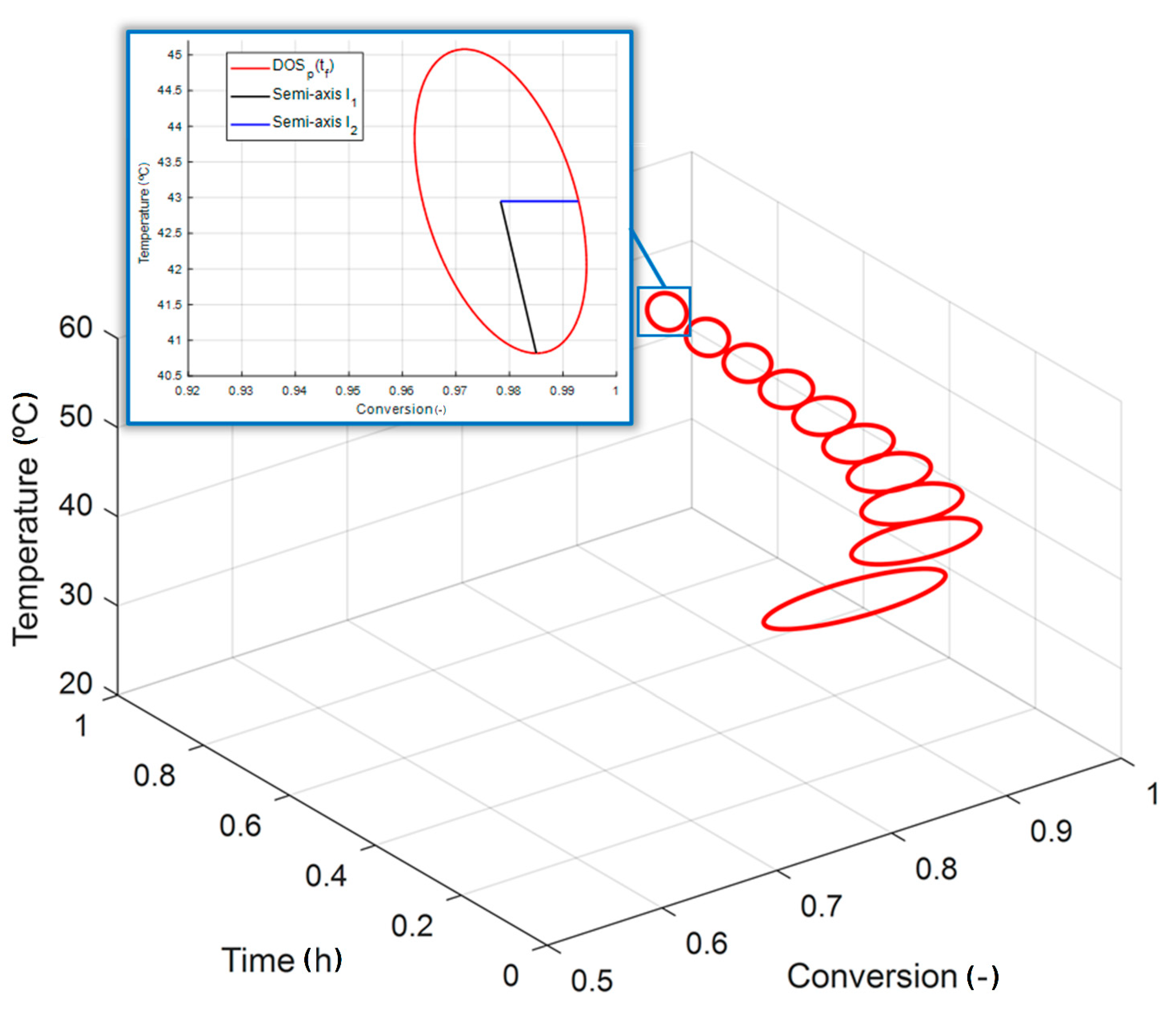
With all outputs indexed by timestamp, the other DOSp(t)s can be calculated from this final point, with the indexed data shown in Figure 13.
In the magnified portion in Figure 13, the shape of the joint reliability region is still closer to an ellipse at the end of the batch, which indicates a strong correlation between temperature and conversion. The funnel-like behavior shown in the figure indicates more desirable possibilities with a higher probability of occurrence at the beginning of the process, followed by the reduction of such possibilities at each time step. This response is due to the fact that the batch is a time-dependent process that relies on cumulative state-changing behavior along the operation (t). Such a process, thus, becomes more difficult to operate as it evolves, as also reflected in the decreasing OI(t) values in Table 2.
Similarly to the classical operability analysis, the intersections between the AOS(t)s and DOSp(t)s can be evaluated at each timestamp over the batch campaign to provide a graphical idea (as shown in Figure 14) of how much the desired output set is achievable and where to operate the process in order to guarantee the final specifications would be reachable. In particular, the black marker in Figure 14 exemplifies an operation sample of a batch in which the specifications were achieved, even considering the random disturbances. Thus, this process can be characterized as fully dynamically operable in terms of reactor conversion and temperature specifications.
In case of deviation from the dashed area in Figure 14, the series of regions would serve as a path for the operation to drive the process back to the proper DOSp(t). In order to drive the process back to the desired region in this case, a control system (such as classical feedback or advanced model predictive control) would be required.
7. Conclusions
The dynamic operability approach introduced here was applied to a strictly time-dependent process. The developed method consists of an extension of the classical operability concepts to a scenario where process dynamics and disturbance statistics are considered. The statistical concepts explored included multivariate normal distributions and probabilistic analysis of the expected disturbance set (EDS). A new desired output set (DOSp(t)) was proposed based on the joint reliability region in which the tolerance value α definition is necessary. A procedure to generate a dynamic design space for a batch process in the form of a sequence of regions was provided and can be used in practice to assist batch process operations, monitoring, and control. Such regions consist of desirable and achievable sets at each time step, considering the constraints and the disturbances being assumed as normally distributed. The product specifications are guaranteed at the end of the process if operated inside the intersection series between the AOS and DOS regions.
The process model developed for the performed batch case study was validated with experiments from a pilot plant. This model was defined as the digital twin for the batch process, and an automated digital experimentation strategy was proposed in an Industry 4.0 framework. The success of the analysis performed here depends on the data source reliability and quality generated by the digital twin. The methodology accuracy is improved as more data are available, and from this perspective a plant information management system (PIMS) can be a powerful tool for operability studies. In future work, the authors plan to integrate the current solution with alarms and message notifications whenever the dynamic operability methodology detects operational actions necessary for the process to return to an operable state.
Author Contributions
This paper is a collaborative work among the authors. W.R.d.A. performed all simulations and wrote the manuscript. H.B. and F.V.L. helped with the analysis and supervision of the research work and with the paper writing and oversaw all technical aspects. All authors have read and agreed to the published version of the manuscript.
Funding
This study was financed in part by the Coordenação de Aperfeiçoamento de Pessoal de Nível Superior—Brazil (CAPES)—Finance Code 001.
Institutional Review Board Statement
Not applicable.
Informed Consent Statement
Not applicable.
Data Availability Statement
Not applicable.
Acknowledgments
The authors thank the Chemical Engineering Department at the Federal University of Campina Grande for the instrumentation and materials used for experiments.
Conflicts of Interest
The authors declare no conflict of interest.
Appendix A

Table A1.
Different disturbances in EDSp(t) in the dynamic operability analysis.
| N | Disturbance | % of Beginning | Intensity from Nominal Value | Time Span (min) |
|---|---|---|---|---|
| 1 | d1 (mL) | 0 | 9.70 | 0 |
| 2 | 0 | −12.24 | 0 | |
| 3 | 0 | −16.43 | 0 | |
| 4 | d2 (mL) | 0 | −73.81 | 0 |
| 5 | 0 | 49.99 | 0 | |
| 6 | 0 | −15.66 | 0 | |
| 7 | d3 (°C) | 0 | 1.52 | 5 |
| 8 | 0 | 1.52 | 15 | |
| 9 | 0 | 1.52 | 30 | |
| 10 | 0 | −3.15 | 5 | |
| 11 | 0 | −3.15 | 15 | |
| 12 | 0 | −3.15 | 30 | |
| 13 | 0 | 4.17 | 5 | |
| 14 | 0 | 4.17 | 15 | |
| 15 | 0 | 4.17 | 30 | |
| 16 | 25 | 1.52 | 5 | |
| 17 | 25 | 1.52 | 15 | |
| 18 | 25 | 1.52 | 30 | |
| 19 | 25 | −3.15 | 5 | |
| 20 | 25 | −3.15 | 15 | |
| 21 | 25 | −3.15 | 30 | |
| 22 | 25 | 4.17 | 5 | |
| 23 | 25 | 4.17 | 15 | |
| 24 | 25 | 4.17 | 30 | |
| 25 | 50 | 1.52 | 5 | |
| 26 | 50 | 1.52 | 15 | |
| 27 | 50 | 1.52 | 30 | |
| 28 | 50 | −3.15 | 5 | |
| 29 | 50 | −3.15 | 15 | |
| 30 | 50 | −3.15 | 30 | |
| 31 | 50 | 4.17 | 5 | |
| 32 | 50 | 4.17 | 15 | |
| 33 | 50 | 4.17 | 30 | |
| 34 | 75 | 1.52 | 5 | |
| 35 | 75 | 1.52 | 15 | |
| 36 | 75 | −3.15 | 5 | |
| 37 | 75 | −3.15 | 15 | |
| 38 | 75 | 4.17 | 5 | |
| 39 | 75 | 4.17 | 15 |
References
- Vinson, D.R.; Georgakis, C. A new measure of process output controllability. J. Process Control 2000, 10, 185–194. [Google Scholar] [CrossRef]
- Lima, F.V.; Jia, Z.; Ierapetritou, M.; Georgakis, C. Similarities and Differences between the Concepts of Operability and Flexibility: The Steady-State Case. AIChE J. 2010, 56, 702–716. [Google Scholar] [CrossRef]
- Carrasco, J.C.; Lima, F.V. Bilevel and Parallel Programing-Based Operability Approaches for Process Intensification and Modularity. AIChE J. 2018, 64, 3042–3054. [Google Scholar] [CrossRef]
- Shead, L.R.E.; Anastassakis, C.G.; Rossiter, J.A. Steady-state operability of multi-variable non-square systems: Application to Model Predictive Control (MPC) of the Shell Heavy Oil Fractionator (SHOF). In Proceedings of the 2007 Mediterranean Conference on Control & Automation, Athens, Greece, 27–29 June 2007; pp. 1–6. [Google Scholar]
- Lima, F.V.; Georgakis, C.; Smith, J.F.; Schnelle, P.D.; Vinson, D.R. Operability-Based Determination of Feasible Control Constraints for Several High-Dimensional Nonsquare Industrial Processes. AIChE J. 2010, 56, 1249–1261. [Google Scholar] [CrossRef]
- Carrasco, J.C.; Lima, F.V. An optimization-based operability framework for process design and intensification of modular natural gas utilization systems. Comput. Chem. Eng. 2017, 105, 246–258. [Google Scholar] [CrossRef]
- Bishop, B.A.; Lima, F.V. Modeling, Simulation, and Operability Analysis of a Nonisothermal, Countercurrent, Polymer Membrane Reactor. Processes 2020, 8, 78. [Google Scholar] [CrossRef] [Green Version]
- Carrasco, J.C.; Lima, F.V. Nonlinear Operability of a Membrane Reactor for Direct Methane Aromatization. In Proceedings of the 9th IFAC ADCHEM Symposium, Whistler, BC, Canada, 7–10 June 2015; Volume 48, pp. 728–733. [Google Scholar]
- Gazzaneo, V.; Carrasco, J.C.; Vinson, D.R.; Lima, F.V. Process Operability Algorithms: Past, Present, and Future Developments. Ind. Eng. Chem. Res. 2020, 59, 2457–2470. [Google Scholar] [CrossRef]
- Subramanian, S.; Georgakis, C. Steady-state operability characteristics of idealized reactors. Chem. Eng. Sci. 2001, 56, 5111–5130. [Google Scholar] [CrossRef]
- Lima, F.V.; Georgakis, C. Design of output constraints for model-based non-square controllers using interval operability. J. Process Control 2008, 18, 610–620. [Google Scholar] [CrossRef]
- Lima, F.V.; Georgakis, C. Input–Output Operability of Control Systems: The Steady-State Case. J. Process Control 2010, 20, 769–776. [Google Scholar] [CrossRef]
- Georgakis, C.; Uztürk, D.; Subramanian, S.; Vinson, D.R. On the operability of continuous processes. Control Eng. Pract. 2003, 11, 859–869. [Google Scholar] [CrossRef]
- Uztürk, D.; Georgakis, C. Inherent Dynamic Operability of Processes: General Definitions and Analysis of SISO Cases. Ind. Eng. Chem. Res. 2002, 41, 421–432. [Google Scholar] [CrossRef]
- Gazzaneo, V.; Lima, F.V. Multilayer Operability Framework for Process Design, Intensification, and Modularization of Nonlinear Energy Systems. Ind. Eng. Chem. Res. 2019, 58, 6069–6079. [Google Scholar] [CrossRef]
- Lima, F.V.; Georgakis, C. Dynamic Operability for the Calculation of Transient Output Constraints for Non-Square Linear Model Predictive Controllers. In Proceedings of the 7th IFAC ADCHEM Symposium, Istanbul, Turkey, 12–15 July 2009; Volume 42, pp. 231–236. [Google Scholar]
- Chen, Y.; Durango-Cohen, P.L. Development and Field Application of a Multivariate Statistical Process Control Framework for Health-Monitoring of Transportation Infrastructure. Transp. Res. Part B Methodol. 2015, 81, 78–102. [Google Scholar] [CrossRef]
- Kharbach, M.; Cherrah, Y.; Heyden, Y.V.; Bouklouze, A. Multivariate Statistical Process Control in Product Quality Review Assessment—A Case Study. Ann. Pharm. Françaises 2017, 75, 446–454. [Google Scholar] [CrossRef] [PubMed]
- Almeida, F.A.; Leite, R.R.; Gomes, G.F.; Gomes, J.H.F.; Paiva, A.P. Multivariate Data Quality Assessment Based on Rotated Factor Scores and Confidence Ellipsoids. Decis. Support Syst. 2020, 129, 113173. [Google Scholar] [CrossRef]
- Soroush, M.; Kravaris, C. Optimal design and operation of batch reactors. 1. Theoretical framework. Ind. Eng. Chem. Res. 1993, 32, 866–881. [Google Scholar] [CrossRef]
- Soroush, M.; Kravaris, C. Optimal design and operation of batch reactors. 2. A case study. Ind. Eng. Chem. Res. 1993, 32, 882–893. [Google Scholar] [CrossRef]
- Herceg, M.; Kvasnica, M.; Jones, C.N.; Morari, M. Multi-Parametric Toolbox 3.0. In Proceedings of the European Control Conference, Zurich, Switzerland, 17–19 July 2013; pp. 502–510. [Google Scholar]
- STAT 505: Applied Multivariate Statistical Analysis. Available online: https://onlinecourses.science.psu.edu/stat505/ (accessed on 15 May 2020).
- Das, K.; Sahoo, P.; Baba, M.S.; Murali, N.; Swaminathan, P. Kinetic studies on saponification of ethyl acetate using an innovative conductivity-monitoring instrument with a pulsating sensor. Int. J. Chem. Kinet. 2011, 43, 648–656. [Google Scholar] [CrossRef]
Figure 1.
Representation of a generic process model for operability with inputs, disturbances, and outputs.
Figure 1.
Representation of a generic process model for operability with inputs, disturbances, and outputs.

Figure 2.
Representation of assumed disturbance behavior.

Figure 3.
Example of a bivariate normal distribution in the shape of an ellipse (adapted from [23]).
Figure 3.
Example of a bivariate normal distribution in the shape of an ellipse (adapted from [23]).

Figure 4.
Experimental apparatus associated with the batch reactor case study.

Figure 5.
Automated digital experimentation flowchart.

Figure 6.
Grid organization for data responses organized by experiment and time.

Figure 7.
Work flow for dynamic operability algorithm.

Figure 8.
Comparison between experimental and simulated results for different ethyl acetate initial concentrations. (a) Molar concentration of sodium hydroxide. (b) Reactor temperature profile.
Figure 8.
Comparison between experimental and simulated results for different ethyl acetate initial concentrations. (a) Molar concentration of sodium hydroxide. (b) Reactor temperature profile.

Figure 9.
Comparison between experimental and simulated results for setpoint reactor temperature sensitivity analysis. (a) Molar concentration of sodium hydroxide. (b) Reactor temperature profile.
Figure 9.
Comparison between experimental and simulated results for setpoint reactor temperature sensitivity analysis. (a) Molar concentration of sodium hydroxide. (b) Reactor temperature profile.

Figure 10.
Points and boundary contours of the achievable output sets at t = 0.1 h. (a) Region representing the initial condition (no disturbance) in black and disturbance #1 (Table A1) in blue. (b) All AOS(d,t = 0.1 h)s determined at 0.1 h and AOS(t = 0.1 h).
Figure 10.
Points and boundary contours of the achievable output sets at t = 0.1 h. (a) Region representing the initial condition (no disturbance) in black and disturbance #1 (Table A1) in blue. (b) All AOS(d,t = 0.1 h)s determined at 0.1 h and AOS(t = 0.1 h).

Figure 11.
Achievable output sets drawn along the batch. (a) Output points, AOS(d,t)s, and AOS(t)s determined at all timestamps considered. (b) AOS(t)s separated for visualization purposes.
Figure 11.
Achievable output sets drawn along the batch. (a) Output points, AOS(d,t)s, and AOS(t)s determined at all timestamps considered. (b) AOS(t)s separated for visualization purposes.

Figure 12.
Construction of the DOSp(t = 1h) based on the DOS() defined by specifications.

Figure 13.
The calculated sequence of DOSp(t)s resulting in funnel-like behavior. This sequence can be used to define regions for batch monitoring and control purposes.
Figure 13.
The calculated sequence of DOSp(t)s resulting in funnel-like behavior. This sequence can be used to define regions for batch monitoring and control purposes.

Figure 14.
Dynamic operability analysis: AOS(t)s, DOSp(t)s, and their intersections over the batch operation. The shaded areas along the campaign represent how much the desired set is achievable.
Figure 14.
Dynamic operability analysis: AOS(t)s, DOSp(t)s, and their intersections over the batch operation. The shaded areas along the campaign represent how much the desired set is achievable.

Table 1.
Categorization of variables in the AIS and EDS.
| Category | Variable | Description |
|---|---|---|
| Static | Ethyl acetate initial molar concentration () | |
| Sodium hydroxide initial molar concentration () | ||
| Initial reactor temperature () | ||
| Sodium hydroxide initial volume () | ||
| Ethyl acetate initial volume () | ||
| Dynamic | Inlet mass flow of the heating fluid () | |
| Inlet temperature of the heating fluid () |
Table 2.
Operability index calculated along batch timestamps.
| t (h) | |||
|---|---|---|---|
| 0.00 | 0 | 0 | - |
| 0.10 | 4.6075 | 0.5359 | 99.93% |
| 0.20 | 3.3821 | 0.3740 | 84.05% |
| 0.30 | 2.2572 | 0.2898 | 68.23% |
| 0.40 | 1.5442 | 0.2373 | 54.86% |
| 0.50 | 1.1098 | 0.2006 | 45.09% |
| 0.60 | 0.8248 | 0.1731 | 37.22% |
| 0.70 | 0.6333 | 0.1522 | 31.02% |
| 0.80 | 0.6308 | 0.1359 | 38.23% |
| 0.90 | 0.6307 | 0.1222 | 45.13% |
| 1.00 | 0.6307 | 0.1119 | 51.82% |
Publisher’s Note: MDPI stays neutral with regard to jurisdictional claims in published maps and institutional affiliations. |
© 2021 by the authors. Licensee MDPI, Basel, Switzerland. This article is an open access article distributed under the terms and conditions of the Creative Commons Attribution (CC BY) license (http://creativecommons.org/licenses/by/4.0/).
Share and Cite
MDPI and ACS Style
de Araujo, W.R.; Lima, F.V.; Bispo, H. Dynamic and Statistical Operability of an Experimental Batch Process. Processes 2021, 9, 441. https://0-doi-org.brum.beds.ac.uk/10.3390/pr9030441
AMA Style
de Araujo WR, Lima FV, Bispo H. Dynamic and Statistical Operability of an Experimental Batch Process. Processes. 2021; 9(3):441. https://0-doi-org.brum.beds.ac.uk/10.3390/pr9030441
Chicago/Turabian Stylede Araujo, Willy R., Fernando V. Lima, and Heleno Bispo. 2021. "Dynamic and Statistical Operability of an Experimental Batch Process" Processes 9, no. 3: 441. https://0-doi-org.brum.beds.ac.uk/10.3390/pr9030441
Note that from the first issue of 2016, this journal uses article numbers instead of page numbers. See further details here.