Process Performance Verification Using Viability Theory ^†

Abstract

The development of efficient methods for process performance verification has drawn a lot of attention in the research community. Viability theory is a mathematical tool to identify the trajectories of a dynamical system which remains in a constraint set. In this paper, viability theory is investigated for this purpose in the case of nonlinear processes that can be represented in Linear Parameter Varying (LPV) form. In particular, verification algorithms based on the use of invariance and viability kernels and capture basin are proposed. The difficulty with the application of this theory is the computation of these sets. A Lagrangian method has been used to approximate these sets. Because of simplicity and efficient computations, zonotopes are adopted for set representation. Two new sets called Safe Work Area (SWA) and Required Performance (RP) are defined and an algorithm is proposed to use these concepts for the verification purpose. Finally, two application examples based on well-known case studies, a two-tank system and PH neutralization plant, are provided to show the effectiveness of the proposed method.

1. Introduction

The objective of process design is that the process achieves the desired dynamical behavior specified in terms of a set of specifications. Therefore, it must be verified that the desired behavior is achievable or not [1]. The complexity of modern process as well as the required performance are increasing. Developing a tool that can guarantee the desired process behavior becomes an interesting area of research. A formal process verification method should provide an answer to the following problem

Problem 1.

Given a process model and a specification of allowed and required behavior, determine if the possible behaviors of the process comply with the specifications.

In other words, formal verification tries to prove the correctness of a process behavior with respect to the associated specifications. This task is a difficult problem to solve in general; it can be solved for certain classes of processes and specifications [1]. There is a trade-off between the complexity of process model and complexity of specifications to be checked, i.e., complex specifications can be verified for simple processes and vice versa, simple specifications can be verified for complex processes. Therefore, most of the methods for verification in complex processes rely on some degree of approximation which may give an inconclusive answer to Problem 1.

Because of difficulties in formal process verification, sometimes it is interesting to verify the safety of the process. A malfunction in safety-critical processes can have catastrophic consequences, hence there is a need to verify safety specifications of the process. Safety verification can be provided by answering to the following problem

Problem 2.

Given a process model and some non-safe regions, determine if the process can reach non-safe regions.

There are two main approaches into process verification: direct and indirect methods [1]. The difference between these two families of approaches is that in direct methods the whole model is considered, while a simplified or abstract model of the process is considered in indirect verification. Reachability analysis is widely used in this area as an acceptable tool for process verification [2]. Safety of the process is a major issue that is investigated using reachability analysis [3]. Another method uses the concepts of abstraction and refinement. First, a simplified hybrid model is generated (abstraction). Then, a search for finding an evolution violating the safety conditions is conducted to refine abstraction [4,5].

There are also some computational tools for checking the system behavior especially in the context of hybrid systems. Uppaal is a toolbox for verification of real-time systems that has been applied successfully in many applications [6]. Hytech is a symbolic model checker for linear hybrid automata which can perform parametric analysis [7]. Checkmate is also a program package which accepts simulated event files in many formats and models [8]. Verification has been successfully treated in many control systems, including hybrid systems, cyber-physical systems, systems consisting of interacting agents, and autonomous systems operating in challenging environments [9]. For example, verification methods have been applied to robot applications [10], avionics [11], railway signaling control system [12], and inverters [13]. In [14], a neuro-fuzzy model is used to assess the performance of a control loop. A survey on the monitoring of industrial control loops performance is presented in [15].

In the literature, the use of sets (and in particular, zonotopes) has also been proposed for systems verification, but in general restricted to the reachability analysis, as e.g., the works of Althoff and Girard, see [16] for a recent review. This paper extends this idea to a more general framework, the viability theory.

Viability theory is a mathematical tool to identify the trajectories of a dynamical system with uncertainty which remains in the viability constraint set, and distinguish them from the trajectories that cross its boundaries [17]. This theory provides a solid framework for control synthesis of constrained dynamical systems in a set-valued fashion [18,19], and has been used in many applications such as robotics [20], aircraft collision avoidance [21] and air traffic management [22]. It also plays an important role in safety verification in control systems, a particular important problem for high-risk, expensive, or safety-critical applications. In many engineering systems, input constraints limit the system’s ability to remain within a desired safe region of operation. For such systems, constraints on the state-space determine the safe set. It is important to identify the subset of the safe set for which the existence of a control input that keeps the states of the system within the safe region can be guaranteed.

In this paper, three concepts in viability theory are used to verify the process performance and safety. These concepts are invariance kernel, viability kernel and capture basin. The main contribution of this paper is an approach for process performance verification using these concepts from viability theory. This approach exploits the relation between concepts in performance verification and viability theory. The difficulty with this theory is related to the computation of the sets involved. Thus, another contribution of this paper is the introduction of algorithms to determine these sets. Because of simplicity and efficient computations, the proposed algorithms are based on zonotopes for set representation and computation, while for process representation the nonlinear system model is brought to a Linear Parameter Varying (LPV) representation. In particular, the process non-linearities are embedded in the system matrices that are not constant but varying with the operating point defined by some measurable process variables. The representation of the nonlinear process model in this way facilitates the set computations based on zonotopes that are required to apply the viability theory to the process performance verification problem. Few of the evaluation and verification algorithms existing presently take into account bounds and constraints of the system explicitly. Another contribution of the proposed method is that bounds and constraints of the system has been considered in computing the viability sets. To illustrate the effectiveness of the process verification approach proposed in this paper, two application examples are provided. A preliminary version of the results of this paper is presented in [23]. Here, an algorithm based.

This paper is organized as follows. In Section 2, some preliminaries about LPV system representation, viability theory concepts and reachability concepts are recalled. In Section 3, the computation of involved sets using zonotopes is detailed in an algorithmic manner for nonlinear systems represented in LPV form. The viability theory approach for process verification is presented in Section 4.2. In Section 5, two case studies based on well-known control benchmarks are used to illustrate the proposed approach. Finally, concluding remarks are provided in Section 6.

2. Preliminary Concepts

2.1. Zonotopic Sets

There exist several families of geometric shapes which can be used to describe convex (or non-convex) sets with varying degrees of accuracy. However, an important limiting factor is the trade-off between the accuracy of the approximation and the complexity of the computations involved, i.e., a particular family may be able to represent a great number of shapes but due to computationally expensive manipulations will be useless in practice. Usually there exists an inverse relation between flexibility of a family and the numerical cost of the representation.

Zonotopes represent a particular class of polytopes which exhibit symmetry with respect to their center. In realistic situations, often the constraints that are given in polytopic form have enough symmetry to be described as zonotopic sets. Even when this is not the case, zonotopic approximations may be constructed. For polytopic sets, [24] gives the tightest zononotopic approximation in fixed directions and [25] introduces an iterative algorithm. In [26], it is proven that any Euclidean ball can be approximated arbitrarily close, in the sense of the Hausdorff distance, by means of a zonotope.

Definition 1

(Minkowski sum). The Minkowski sum of two sets X and Y is defined by

$$X\oplus Y=\left\{x+y:x\in X,y\in Y\right\}$$

Definition 2

(Zonotope). Given a vector $c\in {\mathbb{R}}^n$ (center) and a matrix $H\in {\mathbb{R}}^{n\times m}$ (segment matrix), the set represented as:

$$Z=c\oplus H{\beta }^m=\{c+Hz:z\in {\beta }^m\}$$

is called a zonotope of order m and corresponds to the Minkowski sum of the segments defined by the columns of matrix H. In this expression, ${\beta }^m$ is a unitary box composed by m unitary intervals.

Definition 3

(Interval hull). The interval hull $\square X$ of a closed set X is the smallest interval box that contains X.

Given a zonotope $X=\pi \oplus H{\beta }^{m_z}$, its interval hull can be easily computed by

$$\square X=\left\{x\forall i=1,\cdots ,n:\left|x_i-{\pi }_i\right|⩽{∥H_i∥}_1\right\}$$

where $x_i$ and ${\pi }_i$ are the ith components of x and $\pi$, respectively and $H_i$ is the ith row of H.

Zonotopes have a lot of appealing properties [27]. Some properties that have been used in the following sections are introduced in the Appendix A.

2.2. LPV Representation

LPV systems are a special class of nonlinear systems which appears to be well suited for control and estimation of dynamical systems with parameter variations. This framework was introduced to address the control of nonlinear systems using the extension of powerful linear time-invariant approaches based on linear matrix inequalities (LMIs) [28]. In general, LPV techniques provide a systematic design procedure for gain-scheduled multivariable controllers. The idea of LPV models through parameter nonlinear embedding approach is not to use linearization, but to hide non-linearities into some parameters $\rho$ such that the system can be represented with linear state-space structure. However, since parameters will vary with time, and the resulting LPV model cannot be considered a Linear Time-Invariant (LTI) system and new theory have been developed for the analysis and design [29].

Existing approaches for the LPV modeling of nonlinear systems can be classified into three main categories: linearized-based, state-transformation and nonlinear embedding approach (an automated conversion procedure) [29]. In the first category, nonlinear dynamic system is linearized at several operating points, then the resulting linearized models are interpolated to get a global approximation of the system [30]. State-transformation approaches starts with a priori choice of states and try to apply a coordinate change of the nonlinear state-space representation to get an LPV form [31]. Nonlinear embedding approaches try to rewrite the nonlinear representation in a form where nonlinear terms can be absorbed by varying parameters [32]. The first methodology provides an approximation of the systems with slow variations of the operating point, whereas the others usually produce an exact LPV representation. The last category stands for the automated approaches that try to find an exact LPV representation with least possible conservativeness [29,33]. However, they are computationally intensive algorithms and provide little system theoretic understanding of the choices taken.

In this paper, a discrete-time LPV representation of the nonlinear model is used

$$x\left(t+1\right)=A\left(\rho \left(t\right)\right)x\left(t\right)+B\left(\rho \left(t\right)\right)u\left(t\right)+E\left(\rho \left(t\right)\right)w\left(t\right)$$

(1)

where A, B and E are known matrices of appropriate dimensions that depends on the parameter $\rho \left(t\right)$ that can be measured (or estimated) online. $x\left(t\right)\in X$ is the state, $u\left(t\right)\in U$ is the control input and $w\left(t\right)\in W$ is unknown input (disturbance). The bounding sets X, U and W are defined as

$$\begin{array}{c}X=\left\{x\in {\mathbb{R}}^n:\left|x-x^c\right|⩽\overline{x},x^c\in {\mathbb{R}}^n,\overline{x}\in {\mathbb{R}}^n\right\}\hfill \\ U=\left\{u\in {\mathbb{R}}^m:\left|u-u^c\right|⩽\overline{u},u^c\in {\mathbb{R}}^m,\overline{u}\in {\mathbb{R}}^m\right\}\hfill \\ W=\left\{w\in {\mathbb{R}}^q:\left|w-w^c\right|⩽\overline{w},w^c\in {\mathbb{R}}^q,\overline{w}\in {\mathbb{R}}^q\right\}\hfill \end{array}$$

where $x^c$, $u^c$, $w^c$, $\overline{x}$, $\overline{u}$ and $\overline{w}$ are constant vectors. The set X is a priori known set where the states will always lie. The set U is the set of constraints on the control input signal. It is assumed that the disturbances are unknown but bounded by the set W. These sets can be rewritten as zonotopes

$$\begin{array}{c}X=x^c\oplus H^{\overline{x}}{\beta }^n\hfill \\ U=u^c\oplus H^{\overline{u}}{\beta }^m\hfill \\ W=w^c\oplus H^{\overline{w}}{\beta }^q\hfill \end{array}$$

where $H^{\overline{x}}\in {\mathbb{R}}^{n\times n}$, $H^{\overline{u}}\in {\mathbb{R}}^{m\times m}$ and $H^{\overline{w}}\in {\mathbb{R}}^{q\times q}$ are diagonal matrices with their diagonal entries composed of $\overline{x}$, $\overline{u}$ and $\overline{w}$, respectively. The varying parameters $\rho \left(t\right)$ embed the non-linearities and are function of some system measurable variables known as scheduling variables. Since there exist several possibilities of embedding the non-linearities in the varying parameters $\rho \left(t\right)$, the result of the transformation is non-unique leading to different possible LPV representations. The number of the associated scheduling signals increases rapidly with the system order. As it involves no approximation of the system dynamics, efficient modeling solutions can be achieved in many applications [29,34].

2.3. Viability Theory Concepts

It is assumed that the system (1) is defined in a proper open set $\mathrm{O}\subseteq {\mathbb{R}}^n$ and that there exists a globally defined solution for every initial condition $x\left(0\right)\in \mathrm{O}$. Also, assume that for each $u\left(t\right)\in U$ and $x\left(t\right)\in X$, Equation (1) has a unique solution

$$S\left(t,x,u\right),t\in \mathbb{T}$$

where $S\left(0,x,u\right)=x\left(0\right)$ and $\mathbb{T}$ is a discrete time range $\left[0,\left.\infty \right)\right.$.

Viability theory is concerned with ensuring that the system state remains within a viability constraint set $K\subseteq {\mathbb{R}}^n$. Any trajectory of system (1) that leaves the set K at some point in time is considered to be no longer viable.

Let introduce some viability theory concepts that will be used later in the paper for introducing the proposed process performance assessment methodology:

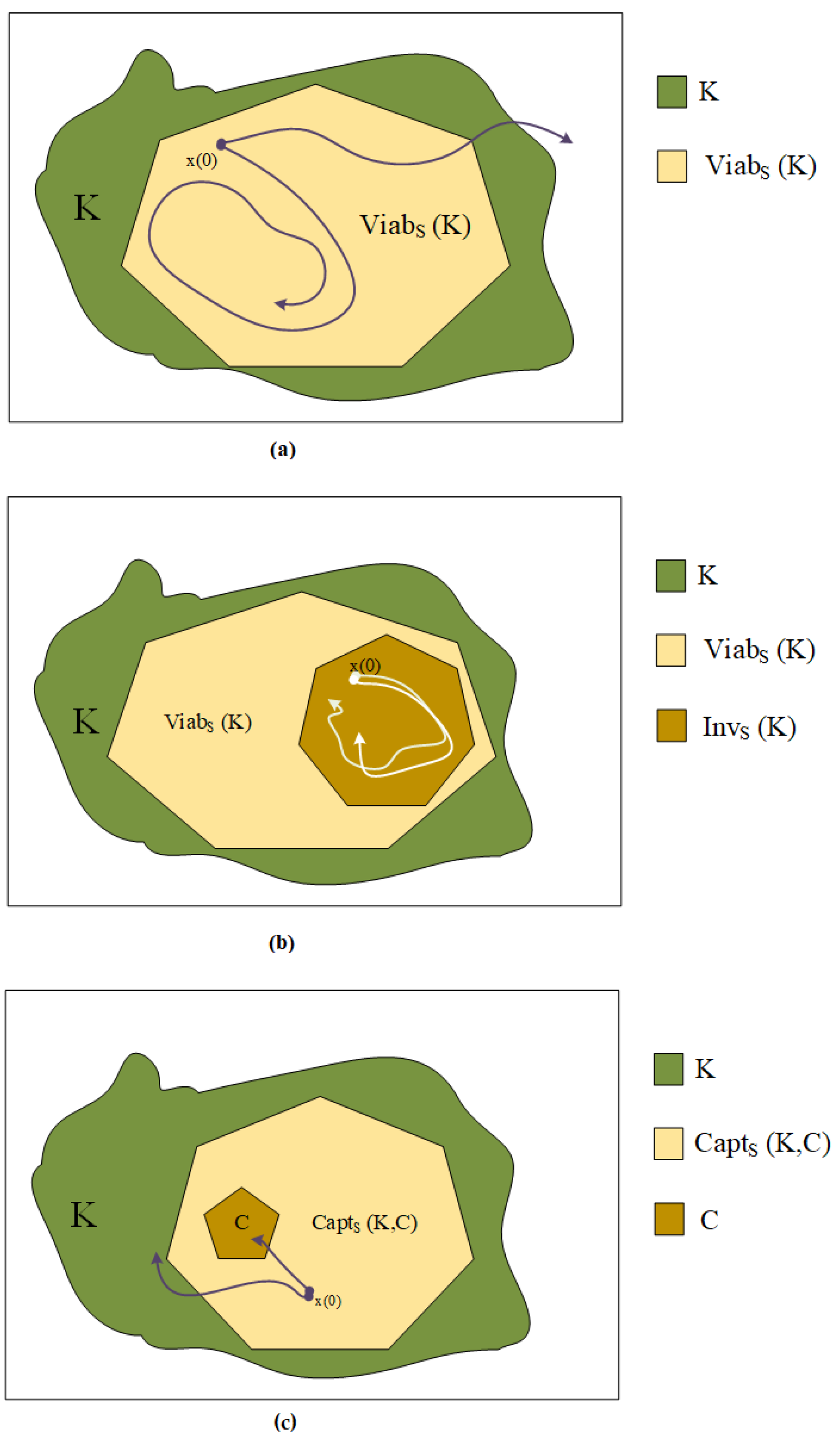
Definition 4

(Viability Kernel). The viability kernel of K under the evolutionary system S is the set $Via{b}_S\left(k\right)$ of initial states $x\left(0\right)\in K$ from which starts at least one evolution $x\left(t\right)\in S\left(x\right)$ viable in K for all times $t\in \mathbb{T}$

$$Via{b}_S\left(K\right)\triangleq \left\{\begin{array}{c}x\left(0\right)\in K|\exists x\left(.\right)\in S\left(x\right)\hfill \\ suchthat\forall t\in \mathbb{T},x\left(t\right)\in K\hfill \end{array}\right\}$$

(2)

This means that from a point $x\left(0\right)$ in the viability kernel of the environment K starts at least one evolution viable in K forever. This is equivalent to say that all evolutions starting from a state belonging to the complement of the viability kernel K leave the environment in finite time. Sometimes, from the engineering point of view, the existence of at least one solution in S is not enough, since nothing is said about all other possible solutions. Therefore, another stronger concept is defined known as the invariance kernel.

Definition 5

(Invariance Kernel). Let $K\subset X$ be an environment. The subset $In{v}_S\left(K\right)$ of initial states $x\left(0\right)\in K$ such that all evolutions $x\left(t\right)\in S\left(x\right)$ starting at $x\left(0\right)$ are viable in K for all $t⩾0$ is called the invariance kernel of K under S

$$In{v}_S\left(K\right)\triangleq \left\{\begin{array}{c}x\left(0\right)\in K|\forall x\left(.\right)\in S\left(x\right),\hfill \\ \forall t\in \mathbb{T},x\left(t\right)\in K\hfill \end{array}\right\}$$

(3)

A state $x\left(0\right)$ belongs to the invariance kernel of the environment K under an evolutionary system S if all the evolutions starting from it are viable in K forever. Despite viability kernel, invariance kernel can guarantee that every system trajectory will remain in the set forever. This concept is widely accepted as a useful tool for fault detection and isolation [35]. Positive invariance in set theory has the same definition as invariance kernel. Viability kernel and weak positive invariance are equivalent definitions in viability and set theories, respectively [19]. Capture basin is another concept that has a wide range of applications, for example, in process control [36] and economics [37].

Definition 6

(Capture Basin). The capture basin of C (viable in K) under the evolutionary system S is the set $Cap{t}_S\left(K,C\right)$ of initial states $x\left(0\right)\in K$ from which starts at least one evolution $x\left(t\right)\in S\left(x\right)$ viable in K on $[0,T)$ until the finite time T when the evolution reaches the target at $x\left(T\right)\in C$.

$$Cap{t}_S\left(K,C\right)\triangleq \left\{\begin{array}{c}x\left(0\right)\in K|\exists x\left(.\right)\in S\left(x\right),\hfill \\ \forall t\in \mathbb{T},x\left(t\right)\in K,x\left(T\right)\in C\hfill \end{array}\right\}$$

(4)

From a state $x\left(0\right)$ in the capture basin of the target C viable in the environment K starts at least one evolution viable in K until it reaches C in finite time. It is equivalent to say that starting from a state belonging to the complement of K, all evolutions remain outside the target C until they leave the environment K. Development of the methods for obtaining these three sets is still an important research area and not an easy task [38]. A conceptual representation of these sets is shown in Figure 1.

2.4. Reachability Concepts

Reachability analysis identifies the set of states backward (forward) reachable by a constrained dynamical system from a given target (initial) set of states. The notions of maximal and minimal reachability analysis were introduced in [39]. Their corresponding constructs differ in how the time variable and the bounded input are quantified. In the formation of the maximal reachability construct, the inputs tries to steer as many states as possible to the target set. On the other hand, in the formation of the minimal reachability construct, the trajectories reach the target set regardless of the input applied. Based on these differences, the maximal and minimal reachable sets and tubes (the set of states traversed by the trajectories over the time horizon [39]) are formed.

In [18,39], it is shown that the minimal reachable tube and the viability kernel are the only constructs that can be used to prove safety of the system and to synthesize inputs (controllers) that preserves it. Since the viability kernel and the minimal reachable tube are dual concepts, they do not need to be treated separately.

Definition 7

(Forward Maximal Reachable Set). The forward maximal reachable set at time instant t is the set of states for which there exists an input such that the trajectories emanating from initial states in R reach that set exactly at time instant t:

$${\mathrm{Reach}}_t^F\left(R\right)\triangleq \left\{x\left(t\right)\in {\mathbb{R}}^n|\exists u\left(.\right)\in U_{\left[0,t\right]},x\left(0\right)\in R\right\}$$

(5)

Definition 8

(Backward Maximal Reachable Set). The backward maximal reachable set at time instant t is the set of initial states for which there exists an input such that the trajectories emanating from those states reach R exactly at time instant t:

$${\mathrm{Reach}}_t^B\left(R\right)\triangleq \left\{x\left(0\right)\in {\mathbb{R}}^n|\exists u\left(.\right)\in U_{\left[0,t\right]},x\left(t\right)\in R\right\}$$

(6)

There are already some references that provide some methods for computing reachable sets using zonotopes, see for example [40,41].

3. Computation of Viability Sets

The difficulty with the application of viability theory to nonlinear systems is due to the computation of the related sets presented in Section 2. In this section, several algorithms are proposed to derive these sets based on zonotopic sets and the LPV representation of the nonlinear system.

3.1. Invariance Kernel Computation

According to Definition 4 and Property 1 in the Appendix , the zonotope $X_t$ that bounds the trajectories of the system (1) at instant t is computed from the previous approximating zonotope at time instant $t-1$, $X_{t-1}=x_{t-1}^c\oplus H_{t-1}^{\overline{x}}{\beta }^n$. Thus,

$${\mathrm{Reach}}_1^F\left(X_{t-1}\right)=X_t=x_t^c\oplus H_t^{\overline{x}}{\beta }^n$$

(7)

where

$$\begin{array}{c}{x}_t^c=mid\left(A\left(\rho \left(t-1\right)\right)\right)x_{t-1}^c+mid\left(B\left(\rho \left(t-1\right)\right)\right)u^c\hfill \\ +mid\left(E\left(\rho \left(t-1\right)\right)\right)w^c\hfill \\ H_t^{\overline{x}}=\left[\begin{array}{cccccc}{J}_1& J_2& J_3& J_4& J_5& J_6\end{array}\right]\hfill \\ J_1=seg\left(◊A\left(\rho \left(t-1\right)\right)H_{t-1}^{\overline{x}}\right)\hfill \\ J_2=\frac{diam\left(A\left(\rho \left(t-1\right)\right)\right)}{2}{x}_{t-1}^c\hfill \\ J_3=seg\left(◊B\left(\rho \left(t-1\right)\right)H^{\overline{u}}\right)\hfill \\ J_4=\frac{diam\left(B\left(\rho \left(t-1\right)\right)\right)}{2}{u}^c\hfill \\ J_5=seg\left(◊E\left(\rho \left(t-1\right)\right)H^{\overline{w}}\right)\hfill \\ J_6=\frac{diam\left(E\left(\rho \left(t-1\right)\right)\right)}{2}{w}^c\hfill \end{array}$$

(8)

where $mid\left(\chi \right)$ and $diam\left(\chi \right)$ denotes, respectively, the center and diameter of the interval matrix $\chi$ element-wise. Zonotopic inclusion operator ◊ is defined in Appendix A. $J_1$, $J_3$ and $J_5$ are calculated using this operator.

Considering $Q=c\oplus H{\beta }^m$ is a zonotope, it is clear that $seg\left(Q\right)=H$. Please note that the set of states has an increasing number of segments generating the zonotope $X_{t+1}$ using this method. To control the domain complexity, a reduction approach must be used. Here, we use the method proposed in [42] to reduce the zonotope complexity. It is also important to note that $\rho \left(t-1\right)$ must be calculated based on information from $x_{t-1}^c$.

The sequence of sets ${\mathrm{Reach}}_1^F\left(X_t\right)$ generated from the dynamic evolution of the system (1) can be determined iteratively to find invariance kernel

$$Inv\left(X\right)=\underset{t=0}{\overset{\infty }{\oplus }}{\mathrm{Reach}}_1^F\left(X_t\right)$$

Algorithm 1 summarizes the calculation of the invariance kernel based on above discussion.

Algorithm 1 Invariance Kernel Estimation

${\displaystyle K_0\leftarrow X}$ $t\leftarrow 1$ while $t⩽N$ do      if $K_t=⌀$ then         $K_N\leftarrow ⌀$         break      end if      if $K_t=K_{t-1}$ then         $K_N\leftarrow K_t$         break      end if      $K_t\leftarrow {\mathrm{Reach}}_1^F\left(K_{t-1}\right)$ (see Equation (7))      $t\leftarrow t+1$ end while return ($K_N$)                                   $K_N=Inv\left(X\right)$

3.2. Viability Kernel Computation

Lagrangian methods have been applied successfully to the computation of reachable sets [43]. In contrast to Eulerian methods, Lagrangian methods use representations that follow the vector field’s flow. Since Lagrangian methods do not depend on gridding the state-space, they are computationally feasible to analyze high-dimensional systems.

In this section, based on [38], a method of expressing finite horizon viability kernels in terms of reachable sets is presented. This provides a modified version of Saint-Pierre’s viability kernel algorithm that can be implemented using efficient and scalable techniques developed within the context of reachability analysis. We can reformulate this recursive definition of the finite horizon viability kernels $K_n$ that is defined as $Via{b}_S$ in (2) but with $\mathbb{T}=\left[0,n\right]$, in terms of the backward reach set over one discrete time step ${\mathrm{Reach}}_t^B\left(X\right)$.

Theorem 1.

The sequence of finite horizon viability kernels $K_n$ can be computed recursively in terms of reach sets as

$$\begin{array}{c}{K}_0=K\hfill \\ K_{t+1}=K_0\cap {Reach}_1^B\left(K_t\right)\hfill \end{array}$$

(9)

Proof. 

See [38]. □

Now, considering nonlinear system expressed in discrete time in the form (1), the backward reachable set over a single time step is computed as

$${\mathrm{Reach}}_1^B\left(X\right)=A{\left(\rho \left(t\right)\right)}^{-1}\{X\oplus \left(-B\left(\rho \left(t\right)\right)\right)U\oplus \left(-E\left(\rho \left(t\right)\right)\right)W\}$$

(10)

Here $A{\left(.\right)}^{-1}$ denotes the pre-image of a set under the map $A:{\mathbb{R}}^d\to {\mathbb{R}}^d$. We will assume that A is non-singular, and thus the pre-image of A can be calculated simply by applying the linear transformation $A{\left(\rho \left(t\right)\right)}^{-1}$ to the set

$$X\oplus \left(-B\left(\rho \left(t\right)\right)\right)U\oplus \left(-E\left(\rho \left(t\right)\right)\right)W$$

This is a fair assumption because we are mainly concerned with discrete time systems that arise from the discretization of continuous time systems. Such systems have a dynamics matrix of the form $A=exp\left(A_{c}t\right)$ which is always invertible.

As the operations required include Minkowski summation, linear transformation and intersection, using the zonotopic representation, there three operations can be performed accurately, efficiently and using a constant amount of memory (see Appendix A). In particular, Equation (8) can be rewritten to calculate backward reach set as

$$\begin{array}{c}{\mathrm{Reach}}_1^B\left(X_t\right)=X_{t-1}=x_{t-1}^c\oplus H_{t-1}^{\overline{x}}{\beta }^n\hfill \\ x_{t-1}^c=mid\left(A{\left(\rho \left(t\right)\right)}^{-1}\right)x_t^c+mid\left(-A{\left(\rho \left(t\right)\right)}^{-1}B\left(\rho \left(t\right)\right)\right)u^c\hfill \\ +mid\left(-A{\left(\rho \left(t\right)\right)}^{-1}E\left(\rho \left(t\right)\right)\right)w^c\hfill \\ H_{t-1}^{\overline{x}}=\left[\begin{array}{cccccc}{J}_1& J_2& J_3& J_4& J_5& J_6\end{array}\right]\hfill \\ J_1=seg\left(◊A{\left(\rho \left(t\right)\right)}^{-1}{H}_t^{\overline{x}}\right)\hfill \\ J_2=\frac{diam\left(A{\left(\rho \left(t\right)\right)}^{-1}\right)}{2}{x}_t^c\hfill \\ J_3=seg\left(◊-A{\left(\rho \left(t\right)\right)}^{-1}B\left(\rho \left(t\right)\right)H^{\overline{u}}\right)\hfill \\ J_4=\frac{diam\left(-A{\left(\rho \left(t\right)\right)}^{-1}B\left(\rho \left(t\right)\right)\right)}{2}{u}^c\hfill \\ J_5=seg\left(◊-A{\left(\rho \left(t\right)\right)}^{-1}E\left(\rho \left(t\right)\right)H^{\overline{w}}\right)\hfill \\ J_6=\frac{diam\left(-A{\left(\rho \left(t\right)\right)}^{-1}E\left(\rho \left(t\right)\right)\right)}{2}{w}^c\hfill \end{array}$$

(11)

This method is similar to the one that is used for invariance kernel computation. The difference is that in invariance kernel computation, the forward reachable set is used, but backward reachable set is used in viability kernel computation.

Algorithm 2 summarizes the calculation of the viability kernel based on the previous explanations.

Algorithm 2 Viability Kernel Estimation

${\displaystyle K_0\leftarrow X}$ $t\leftarrow 1$ while $t⩽N$ do      if $K_t=⌀$ then         $K_N\leftarrow ⌀$         break      end if      if $K_t=K_{t-1}$ then         $K_N\leftarrow K_t$         break      end if      $L\leftarrow {\mathrm{Reach}}_1^B\left(K_{t-1}\right)$ (see Equation (11))      $K_{t+1}\leftarrow K_0\cap L$ (Equation (A1))     $t\leftarrow t+1$ end while return $\left(K_N\right)$                                    $K_N=Viab\left(X\right)$

3.3. Capture Basin Computation

Based on capture basin concept (see Definition 6), it is clear that we can easily adapt Algorithm 2 to compute it. In the viability kernel definition, no time constraint is considered. Therefore, the algorithm is repeated until it converges to a set. However, in the capture basin concept, there is a time limit that can be considered by a small change in the stop criterion of the viability algorithm. Actually, we must find the backward reachable tube for each time instant t. Following this idea, Algorithm 3 is proposed.

Please note that the computed set must lie inside the initial set. Therefore, an intersection of the output of while loop ($K_t$) and initial set (X) is computed at the end of the algorithm.

For Algorithms 1 and 2, N is a big number that assures the algorithm will converge in N steps while it will not go inside an unlimited while loop. In Algorithm 3, the number of time steps is provided in the definition of capture basin as T.

Algorithm 3 Capture Basin Estimation

${\displaystyle K_0\leftarrow C}$ $t\leftarrow 1$ while $t⩽T$ do      if $K_t=⌀$ then         $K_T\leftarrow ⌀$         break      end if      $K_t\leftarrow {\mathrm{Reach}}_1^B\left(K_{t-1}\right)$ (see Equation (11))      $t\leftarrow t+1$ end while $K_N=K_T\cap X$ return $\left(K_N\right)$                                   $K_N=Capt\left(X,C\right)$

4. Process Performance Verification

4.1. Problem Description

As discussed in the introduction, the problem of process verification has recently received increased attention (see e.g., [2,44]) providing the answer to questions as: Is there a potentially unsafe configuration, or state, reachable from an initial configuration? The problem of process performance verification may be encoded as a condition on the region of operation in the system state-space: given a region of the state-space that represents unsafe operation, prove that the set of states from which the system can enter this unsafe region has empty intersection with the system initial states.

The size and shape of these sets depends on the control and disturbance system inputs. Control variables may be chosen to change the sets, whereas the full range of disturbance variables must be taken into account in this computation [2].

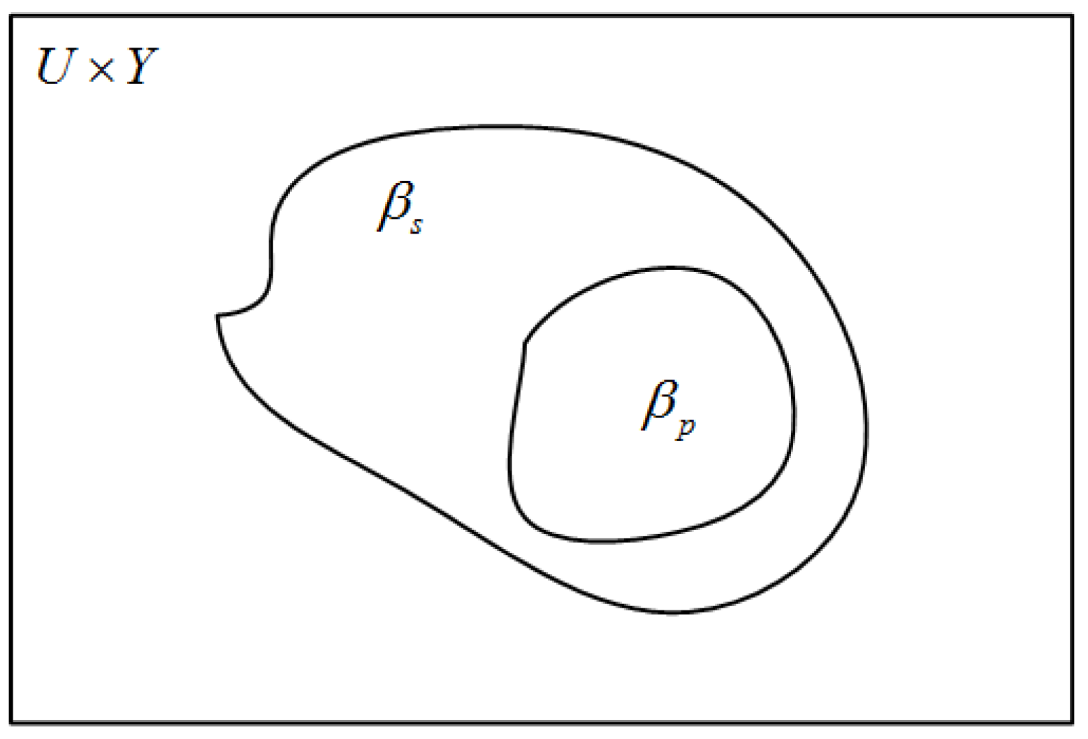
In this paper, the aim is to investigate if the performance requirements of a given process are satisfied. This can be illustrated by using the notion of the process behavior (Figure 2). It is important to associate to which process output $y\left(t\right)$ reacts if a change in a particular input $u\left(t\right)$ is applied. The pair $(u,y)$ is called input-output pair and the set of all possible pair that may occur for a given process define the behavior ${\beta }_p$. The behavior ${\beta }_p$ is a subset of the space $U\times Y$ of all possible combinations of input and output signals [45]. The behavioral requirements of the system can be shown as the ${\beta }_s$ of those I/O pairs. As ${\beta }_p$ lies completely within the set ${\beta }_s$

$${\beta }_p\subset {\beta }_s$$

the process satisfies the considered specifications.

4.2. Process Performance Verification Using Viability Theory

Based on the viability concepts recalled in Section 2 and the algorithms for computing the sets involved presented before, it can be readily deduced that there are some similarities that allow use of viability theory in process performance verification. It is desirable to find equivalency between concepts that until now are used for process verification and those coming from the viability theory.

4.2.1. Safety Verification

The system is required to work in a set that satisfies some given specifications. In safety verification, only parts of trajectories of system (1) that are contained in a given set $X\subseteq {\mathbb{R}}^n$ and that start from a given set $X_0\subseteq X$ of possible initial states are considered. The unsafe region of the system is denoted by $X_u\subseteq X$. With these notations, the safety property can be defined as follows.

Definition 9

(Safety). The safety property holds if there exist no time instant $t\in \left[0,T\right]$ for the considered set of inputs and disturbances

$$\begin{array}{c}u:\left[0,T\right]\to U\hfill \\ w:\left[0,T\right]\to W\hfill \end{array}$$

such that gives rise to an unsafe system trajectory, i.e., a trajectory $x\left(.\right)\in S\left(x\right)$ satisfying $x\left(0\right)\in X_0$, $x\left(T\right)\in X_u$ and $x\left(t\right)\in X$ for all $t\in \left[0,T\right]$.

Initializing the system for every $x\left(0\right)$ inside the viability kernel, there exist a system trajectory that remains inside that kernel. Therefore, if the viability kernel does not intersect with the unsafe set $X_u$, it can be regarded as safe area. The Safe Work Area (SWA) of the system (1) can be represented by

$$SWA=\left\{\left(x,u,w\right)\in \left(X,U,W\right)|\forall t,x\left(t\right)\in Viab\left(X\right)\setminus X_u\right\}$$

(12)

This set conceptually corresponds to ${\beta }_s$ in Figure 2. Therefore, if the system works in the viability kernel, safety requirements are met. In the viability kernel definition, there is a limitation that the system must have at least one evolution that remains in the set. This is close to the concept of stability in Lyapunov theory. The above definition about safety does not consider the performance of the system. In the next section, a performance index is introduced and then, the way of assessing this index using viability concepts is investigated.

4.2.2. Performance Verification

Suppose that the system (1) must reach a desirable set (C) in a given time (T). The performance of the system can be defined as follows.

Definition 10

(Performance). The performance requirements can be met if there exist a time instant $T⩾0$ such that for some inputs and disturbances satisfying

$$\begin{array}{c}u:\left[0,T\right]\to U\hfill \\ w:\left[0,T\right]\to W\hfill \end{array}$$

makes the system to reach a desired set (C) in time T, i.e., there exists a trajectory $x\left(.\right)\in S\left(x\right)$ satisfying $x\left(0\right)\in X_0$, $x\left(T\right)\in C$ and $x\left(t\right)\in X$ for all $t\in \left[0,T\right]$.

To assess if the system performance is acceptable (i.e., satisfies the specifications), the capture basin concept is used. Capture basin is a set that shows the capability of the system to reach a target set (C) in predefined time range. After finding the viability kernel based on state and input constraints, the capture basin can be obtained. The Required Performance ($RP$) for the system (1) can be stated as

$$RP=\left\{\left(x,u,w\right)\in \left(X,U,W\right)|x\left(t\right)\in Capt\left(X,C\right)\right\}$$

(13)

The RP set can be considered to be the plant behavior ${\beta }_p$ in Figure 2. This means that if the system works in the capture basin, it has the capability to arrive to the target in a finite and desired time T that is used in capture basin calculation algorithm. The target corresponds to a small set near steady state set inside viability kernel or a small set around a predefined trajectory. Also, the invariance kernel can be used as target in capture basin computation:

$$C\equiv In{v}_S\left(X\right)$$

4.2.3. Algorithm

Now, after formulating the system verification problem using viability theory concepts, an algorithmic procedure will be provided. The performance evaluation starts obtaining the viability kernel given a set of initial states and the system dynamics. This procedure was described in Algorithm 2 in the previous section. Then, invariance kernel is computed based on the Algorithm 1. After that, capture basin is computed using Algorithm 3 and considering invariance kernel as target and a desired step size. If the capture basin and viability kernel have no empty intersection, it can be said that required performance of the system can be achieved by the control loop if the system starts on that region. The procedure can be repeated for each operation mode of the system. Algorithm 4 shows the procedure for system verification using viability theory concepts.

Algorithm 4 System Verification

Considering the process dynamics (1) and the desired requirements, at each time iteration in the time horizon selected for the analysis:        Determine viability kernel using Algorithm 2      Determine $SWA$ from the viability kernel using Equation (12)     Determine invariance kernel using Algorithm 1      Determine capture basin from the capture basin based on invariance kernel and desired       time steps to reach the target using Algorithm 3      Determine RP using Equation (13)      if $SWA\cap RP\ne ⌀$         if the system starts in $SWA\cap RP$           Process requirements are satisfied         else if the system starts in $SWA$           Process works in safe area         else           Process is not safe         end if      else         Process requirements cannot be satisfied      end if

5. Illustrative Examples

In this section, we provide two examples based on well-known case studies to illustrate how the proposed method can be used in process performance verification.

5.1. Two-Tank System

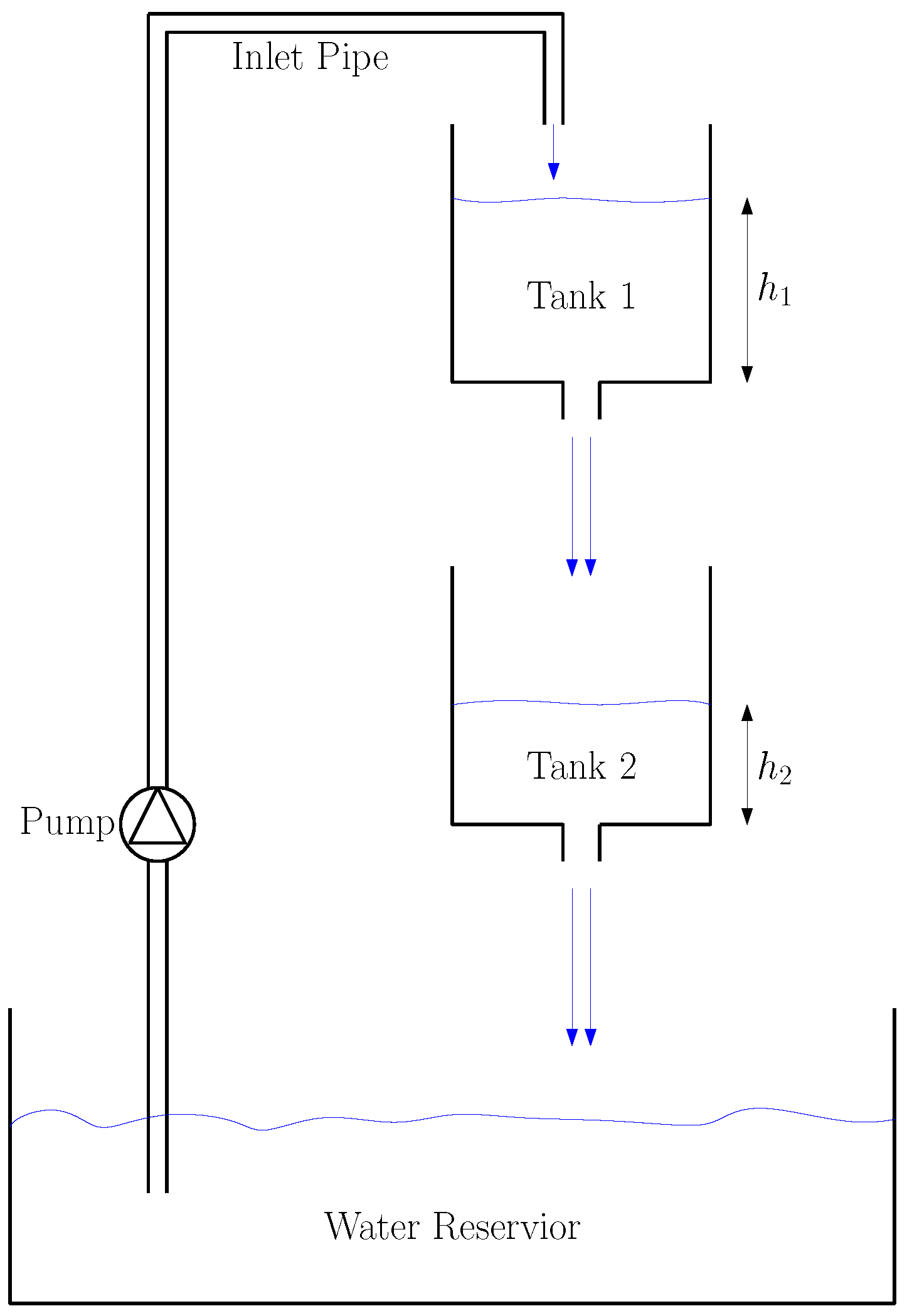
First, the algorithms for system verification developed in the previous sections are applied to a two-tank process that is modeled as a LPV system. The two-tank process is composed of two cylindrical tanks: an upper tank (tank 1) and a lower tank (tank 2), see Figure 3. A pump is used to send water from the water reservoir to tank 1 and the outflow of tank 1 flows through tank 2 to the water reservoir. Pressure sensors located at the bottom of each tank are used to measure the water levels in the tanks. The dynamics model of the water levels $h_1\left(t\right)$ and $h_2\left(t\right)$ can be written as [35]

$$\begin{array}{c}{\dot{h}}_1\left(t\right)=-\left(\frac{s}{S}\right)\sqrt{2g{h}_1\left(t\right)}+\left(\frac{\kappa }{S}\right)u\left(t\right)+w_1\left(t\right)\hfill \\ {\dot{h}}_2\left(t\right)=\left(\frac{s}{S}\right)\sqrt{2g\left(h_1\left(t\right)-h_2\left(t\right)\right)}+w_2\left(t\right)\hfill \end{array}$$

(14)

where $u\left(t\right)$ is the voltage applied to the pump, $h_1\left(t\right)$ and $h_2\left(t\right)$ are system states, $w_1\left(t\right)$, $w_2\left(t\right)$ are bounded state disturbances. The system parameters are as follows: S = 15.5179 cm${}^2$ is the cross-section area of the tanks; s = 0.1781 cm${}^2$ is the cross-section of the tanks outflow orifice; $\kappa$ = 3.3 cm${}^3$ Vs is the gain of the pump; and g = 981 cm/s${}^2$ is the gravitational constant. After Euler discretization with sampling period $\tau =1$ s, the whole system is formulated in LPV form by using the parameter nonlinear embedding approach [46]

$$\begin{array}{c}x\left(t+1\right)=A\left(\rho \left(t\right)\right)x\left(t\right)+Bu\left(t\right)+Ew\left(t\right)\hfill \\ y\left(t\right)=Cx\left(t\right)+\eta \left(t\right)\hfill \end{array}$$

(15)

where

$$\begin{array}{c}x\left(t\right)={\left[\begin{array}{cc}{h}_1\left(t\right)& h_2\left(t\right)\end{array}\right]}^T\hfill \\ A\left(\rho \left(t\right)\right)=I+\tau \left[\begin{array}{cc}-{\rho }_1\left(t\right)& 0\\ {\rho }_1\left(t\right)& -{\rho }_2\left(t\right)\end{array}\right]\hfill \\ B=\tau {\left[\begin{array}{cc}\frac{\kappa }{S}& 0\end{array}\right]}^T\hfill \\ C=\left[\begin{array}{cc}0& 1\end{array}\right]\hfill \\ E=\tau {\left[\begin{array}{cc}1& 1\end{array}\right]}^T\hfill \\ \eta \left(t\right)={\left[\begin{array}{cc}{\eta }_1\left(t\right)& {\eta }_2\left(t\right)\end{array}\right]}^T\hfill \end{array}$$

I is the identity matrix and the varying parameters $\rho$ are defined as follows

$${\rho }_i\left(t\right)=\frac{s}{S}\sqrt{\frac{2g}{h_i\left(t\right)}},i=1,2$$

Therefore, by measuring $h_i$ during the system operation, it is possible to find ${\rho }_i$ online. $\eta \left(t\right)$ is the measurement noise matrix. Disturbances and noises are considered bounded by means of zonotopes with center in 0 and segment of 0.01

$$\begin{array}{cc}\hfill w_i& =0\oplus 0.01\beta ,i=1,2\hfill \\ \hfill {\eta }_i& =0\oplus 0.01\beta ,i=1,2\hfill \end{array}$$

In this system, because the maximum value for states (water height in each tank) is 30 cm, the system must meet the following condition to become safe:

$$x_i\in \left[\begin{array}{cc}0,& 30\end{array}\right],i=1,2$$

Also, let assume that the system must satisfy the following performance requirements:

• The goal is for $h_2\left(t\right)$ to track a reference of 5 cm.
• It must be able to go near the reference in 5 sample times.

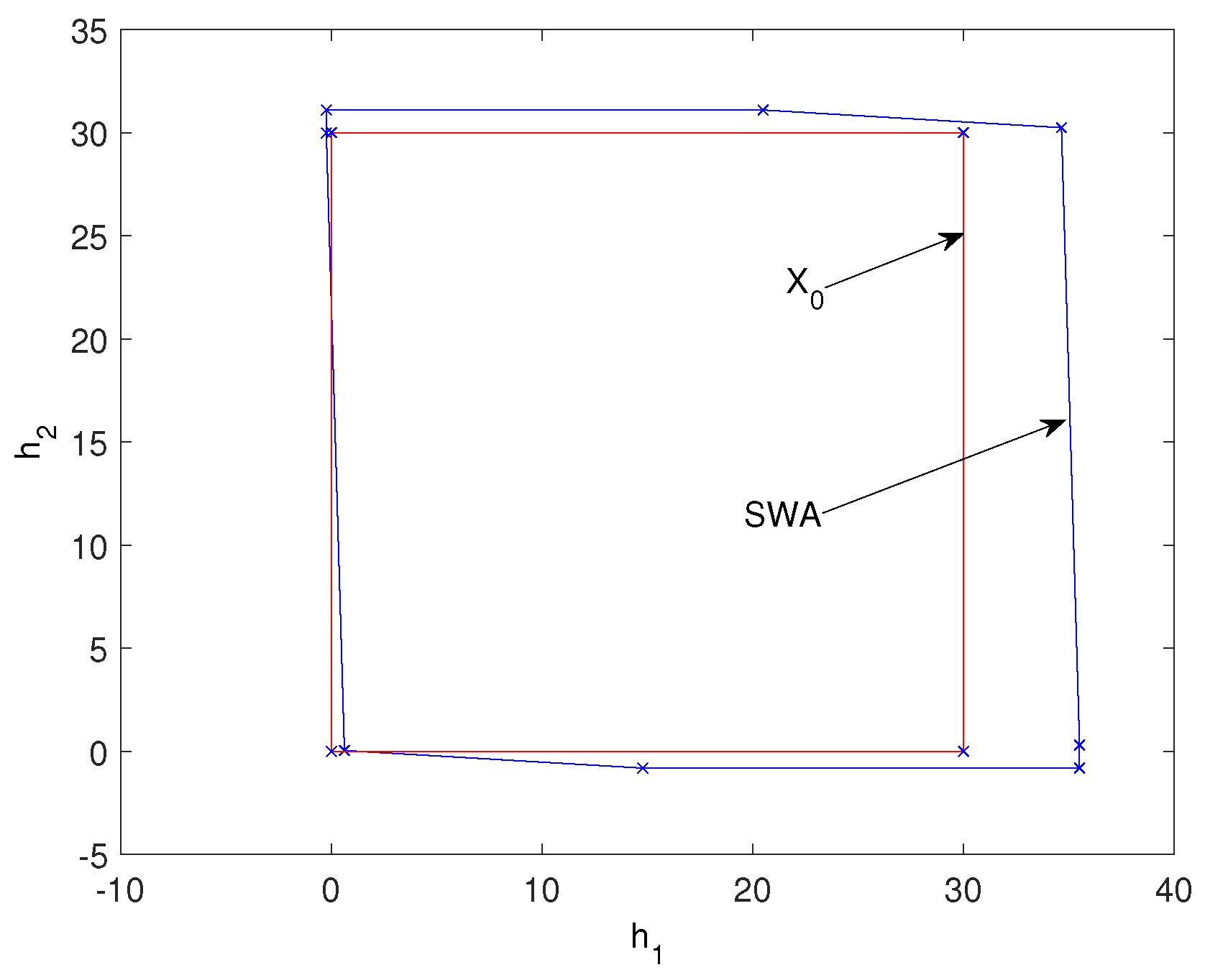
The initial zonotope for system states is chosen to cover all the possible values for states. Accordingly, initial zonotope for states x is considered to be:

$$X_0=\left[\begin{array}{c}15\\ 15\end{array}\right]\oplus \left[\begin{array}{cc}15& 0\\ 0& 15\end{array}\right]{\beta }^2$$

As discussed in Section 4, the viability kernel can be interpreted as a tool for verifying if the system can reach the steady state (see Algorithm 2). As shown in Figure 4, the system is working in SWA. Please note that because there is no unsafe set ($X_u$) in this system, SWA is the same as viability kernel that can be computed using Algorithm 2. Here, because starting from any height there is a possibility to achieve the desired steady state, viability kernel covers all the initial zonotope ($X_0$) approximately. It means that if no time limitation is considered, each state can arrive to its steady state.

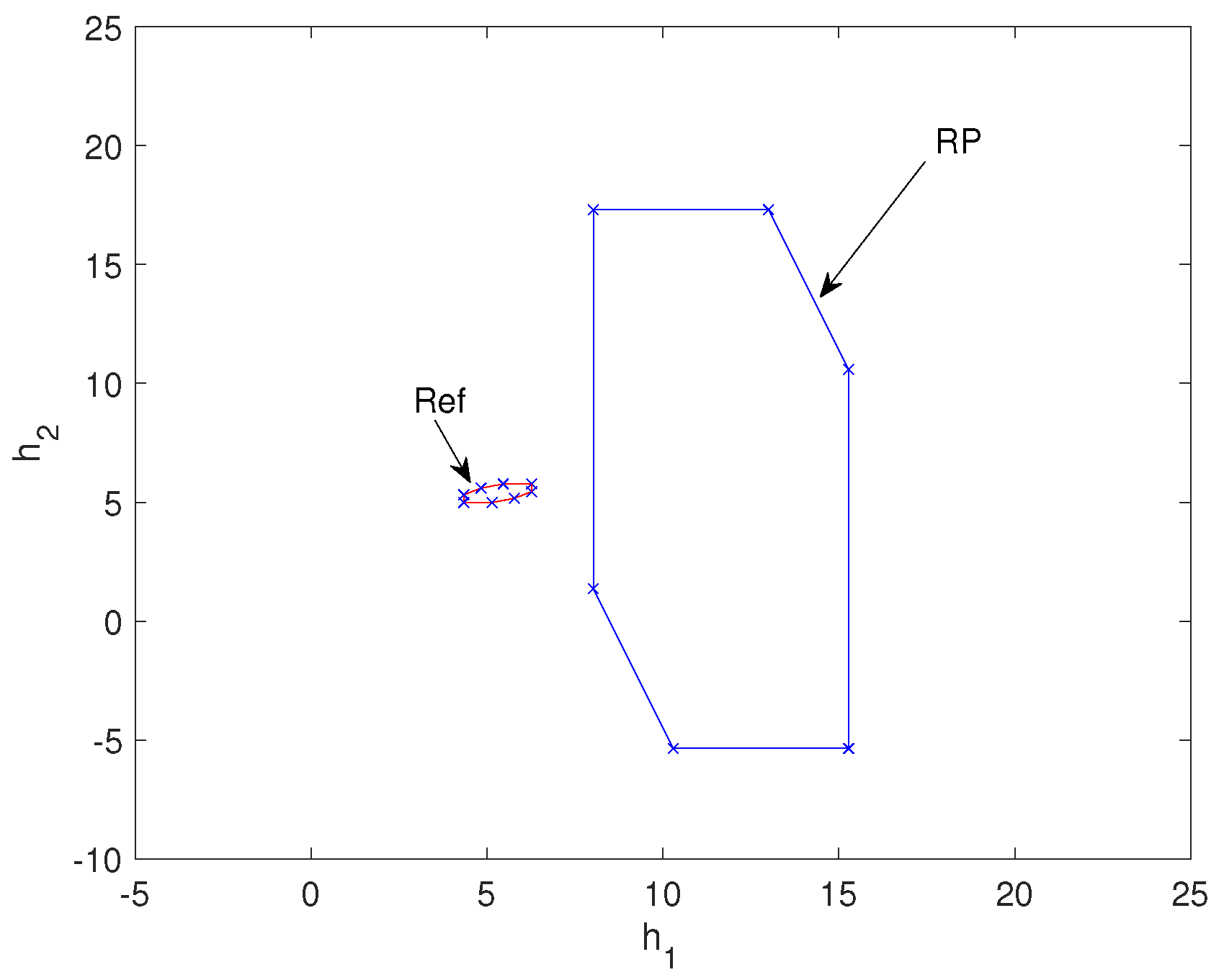
Invariance kernel can be computed using Algorithm 1 that is a set around the steady state of the system. It can be used as a tool for detecting faults in steady state [35]. Also, it can be used as initial set for capture basin construction. Capture basin defining the $RP$ set is computed by means of Algorithm 3 using invariance kernel, denoted as reference (Ref) in Figure 5.

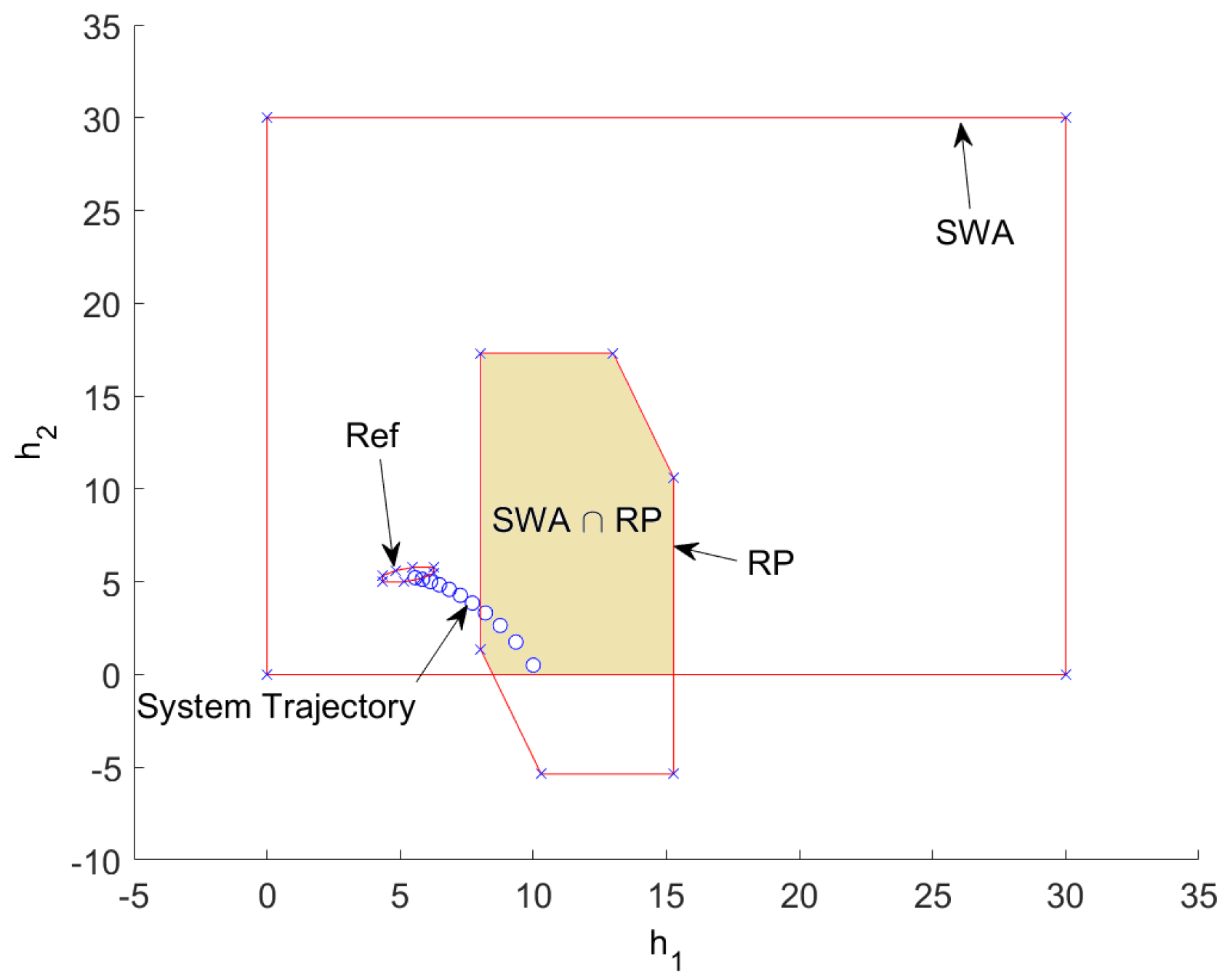
Taking into account that the sampling time of the system $(\tau =1$ s), the system requires 5 s to reach the steady state. Using the $RP$ set, it can be assessed if the system has the possibility to achieve the desired set. It must be pointed out that starting inside $RP$ does not mean that the system will inevitably go to the reference in 5 s. This means that the system can go there in the desired time. According to Algorithm 4, it is required that $RP$ and $SWA$ should not have empty intersection. The intersection of these two sets is shown in Figure 6. In this figure, the system is simulated considering that it starts from $x_0={\left[\begin{array}{cc}10& 0\end{array}\right]}^T$. It is clear that the system goes to the target in about 10 step times, but because it starts in $SWA\cap RP$, it is safe and can go there in 5 step times by using an appropriate controller. However, starting outside this set, there is no possibility to achieve the target in 5 step times.

5.2. PH Neutralization Plant

The second application example is based on a bench-scale PH neutralization plant where an acid stream and an alkaline stream provide a $2.5$ L constant volume to a well-mixed tank. The pH is measured through a sensor located directly in the tank. A mathematical model of this process has been presented in [47]

$$\begin{array}{c}{\dot{x}}_1=\frac{1}{\theta }\left(x_{1,i}-x_1\right)-\frac{1}{\theta }{x}_{1}u\hfill \\ {\dot{x}}_2=\frac{1}{\theta }{x}_2+\frac{1}{\theta }\left(x_{2,i}-x_2\right)u\hfill \\ {\dot{x}}_3=\frac{1}{\theta }{x}_3+\frac{1}{\theta }\left(x_{3,i}-x_3\right)u\hfill \\ h\left(x,y\right)\equiv \xi +x_2+x_3-x_1-\frac{K_w}{\xi }-\frac{x_3}{1+\frac{K_x\xi }{K_w}}=0\hfill \end{array}$$

(16)

The last equation can also be expressed in the polynomial form as follows

$$\begin{array}{c}h\left(x,y\right)\equiv K_x{\xi }^3+\left[K_w+\left(x_3+x_2-x_1\right)K_x\right]{\xi }^2\hfill \\ +\left(x_2-x_1-K_x\right)K_w\xi -K_w^2=0,\hfill \end{array}$$

where $\xi ={10}^{-y}$, $\theta =V/\phantom{V{q}_A}{q}_A$, $u=q_B/\phantom{q_B{q}_A}{q}_A$. The model parameters are given in

Table 1. Model parameters for pH system

Parameter	Value
$x_{1,i}$	0.0012 mol HCl/L
$x_{2,i}$	0.002 mol NaOH/L
$x_{3,i}$	0.0025 mol NaHCO${}_3$/L
$K_x$	${10}^{-7}$ mol/L
$K_w$	${10}^{-14}$ mol${}^2$/L${}^2$
$q_A$	1 L/min (16.67 mL/s)
V	2500 mL

. The system has proven to be a good case study as it exhibits significant nonlinear behavior and model mismatch.

As the proposed algorithms for finding viability sets are formulated in a discrete time scheme, the system (16) can be discretized using Euler discretization method and expressed in the LPV form using the nonlinear embedding approach as follows

$$x\left(t+1\right)=Ax\left(t\right)+B\left(x\left(t\right)\right)u\left(t\right)+Ew\left(t\right)$$

where

$$\begin{array}{c}x\left(t\right)={\left[\begin{array}{ccc}{x}_1\left(t\right)& x_2\left(t\right)& x_3\left(t\right)\end{array}\right]}^T\hfill \\ A=I_{3\times 3}+\tau \left[\begin{array}{ccc}-\frac{1}{\theta }& 0& 0\\ 0& -\frac{1}{\theta }& 0\\ 0& 0& -\frac{1}{\theta }\end{array}\right]\hfill \\ B\left(x\left(t\right)\right)=\tau {\left[\begin{array}{ccc}-\frac{1}{\theta }{x}_1& \frac{1}{\theta }\left(x_{2,i}-x_2\right)& \frac{1}{\theta }\left(x_{3,i}-x_3\right)\end{array}\right]}^T\hfill \\ E=\tau {\left[\begin{array}{ccc}\frac{1}{\theta }{x}_{1,i}& 0& 0\end{array}\right]}^T\hfill \end{array}$$

Initial zonotope of X for finding invariance kernel and SWA is considered to be:

$$X_0=\left[\begin{array}{c}0\\ 0\\ 0\end{array}\right]\oplus \left[\begin{array}{ccc}5\times {10}^{-3}& 0& 0\\ 0& 5\times {10}^{-3}& 0\\ 0& 0& 5\times {10}^{-3}\end{array}\right]{\beta }^3$$

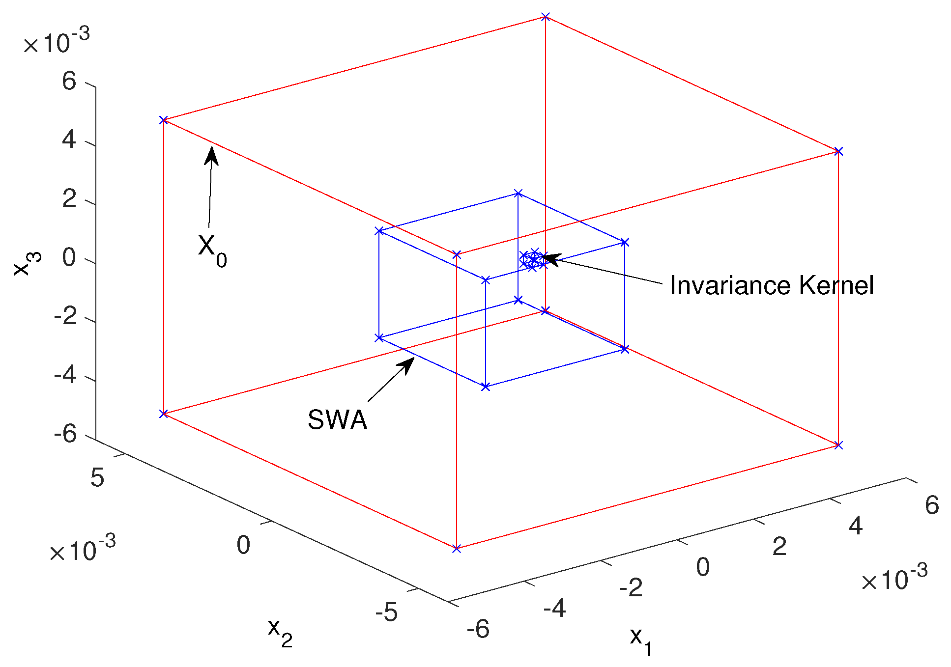
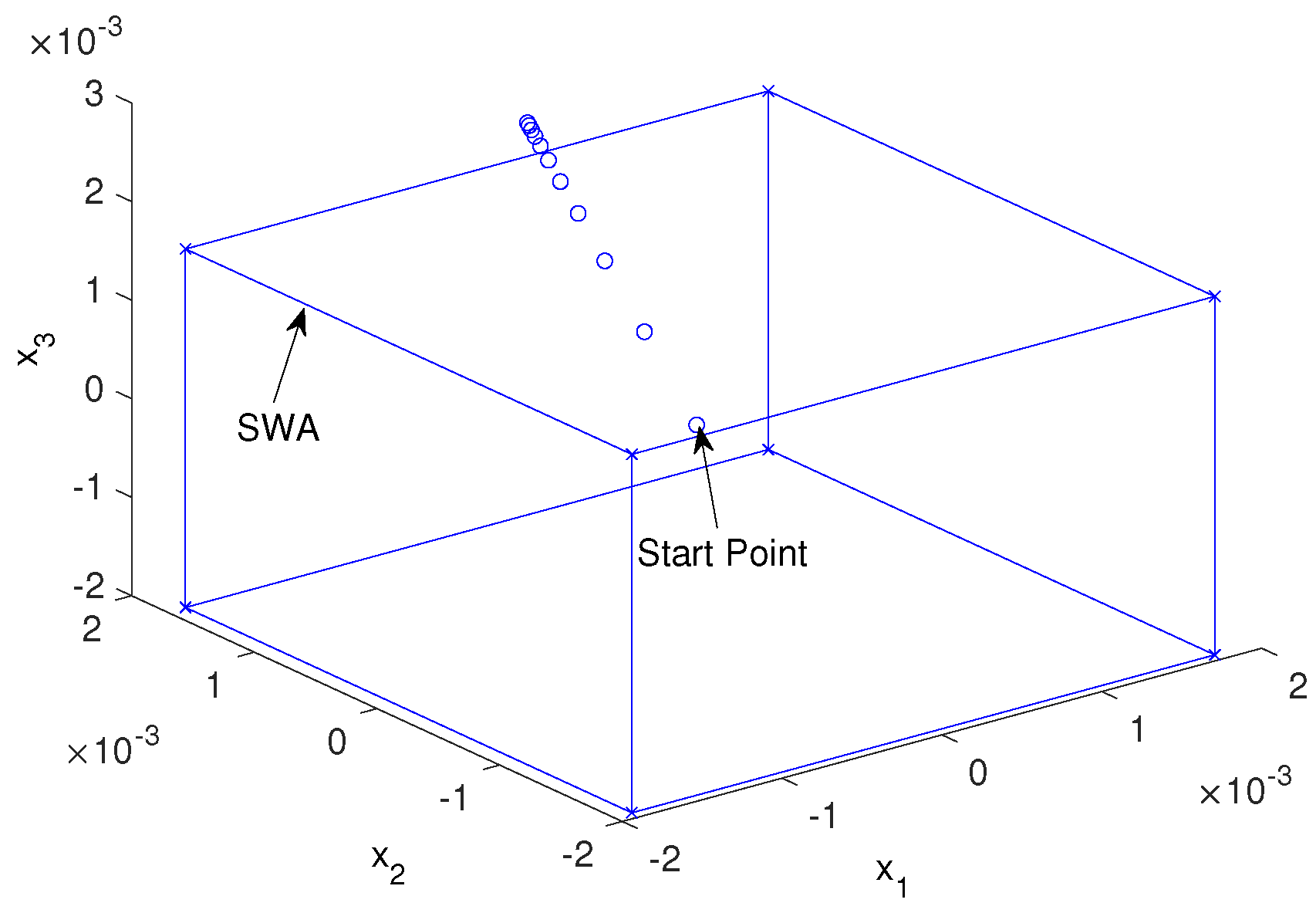
Assume that the required performance in this process is that it must reach the reference in less than 100 s. Considering different values for $\tau$ will change A, B and E values, therefore the size of predefined sets will change. Here, two discretization times are considered: $\tau$ = 1 s and $\tau$ = 5 s. For $\tau$ = 1 s, initial zonotope, invariance kernel and SWA set are drawn in Figure 7. Here, the invariance kernel and SWA are computed using Algorithms 1 and 2, respectively.

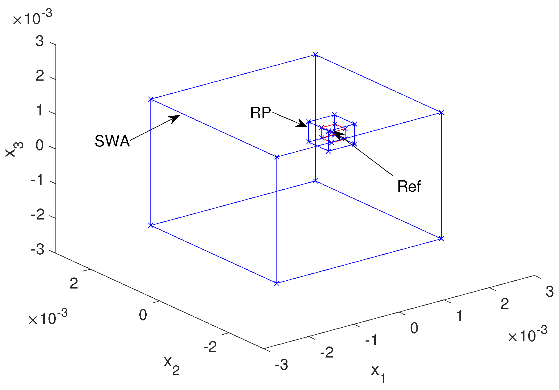
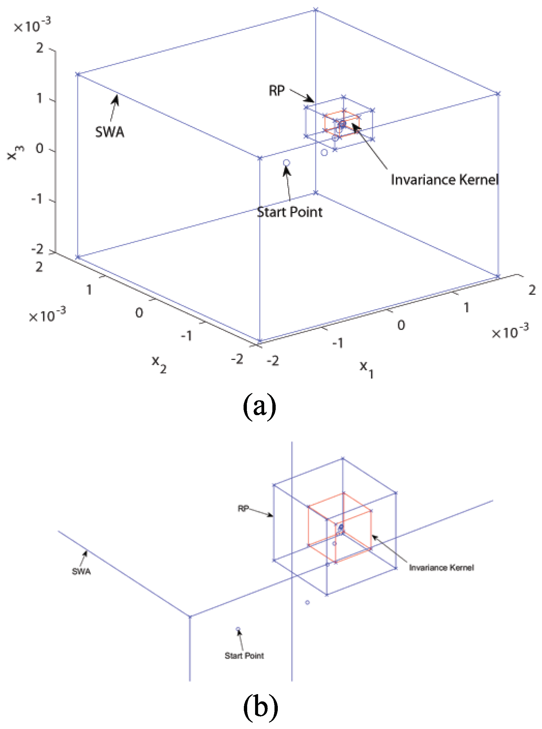
Initial zonotope for $RP$ calculation is the invariance kernel and is shown as Ref in Figure 8. The RP set is calculated by Algorithm 3. If discretization time is assumed to be $\tau$ = 5 s, the sets are calculated in the same way. Because the sets in this case are not very different, the corresponding figure is similar to Figure 7 and Figure 8. For comparison purposes, the definition of the zonotopes corresponding to these sets are provided for these two cases in

Table 2. Calculated sets for different sample times in pH system.

	$\mathit{\tau }=$ 1 s	$\mathit{\tau }=$ 5 s
Ref	$\left[\begin{array}{c}0.0010\\ 2.4072\times {10}^{-4}\\ 3.0090\times {10}^{-4}\end{array}\right]\oplus \left[\begin{array}{ccc}1.4813\times {10}^{-4}& 0& 0\\ 0& 1.4813\times {10}^{-4}& 0\\ 0& 0& 1.4813\times {10}^{-4}\end{array}\right]{\beta }^3$	$\left[\begin{array}{c}0.0010\\ 2.4447\times {10}^{-4}\\ 3.0559\times {10}^{-4}\end{array}\right]\oplus \left[\begin{array}{ccc}2.8879\times {10}^{-5}& 0& 0\\ 0& 2.8879\times {10}^{-5}& 0\\ 0& 0& 2.8879\times {10}^{-5}\end{array}\right]{\beta }^3$
SWA	$\left[\begin{array}{c}-1.5297\times {10}^{-5}\\ -2.5488\times {10}^{-5}\\ -3.1873\times {10}^{-5}\end{array}\right]\oplus \left[\begin{array}{ccc}0.0017& 0& 0\\ 0& 0.0017& 0\\ 0& 0& 0.0017\end{array}\right]{\beta }^3$	$\left[\begin{array}{c}-7.8933\times {10}^{-5}\\ -1.3147\times {10}^{-4}\\ -1.6437\times {10}^{-4}\end{array}\right]\oplus \left[\begin{array}{ccc}0.0018& 0& 0\\ 0& 0.0018& 0\\ 0& 0& 0.0018\end{array}\right]{\beta }^3$
RP	$\left[\begin{array}{c}0.0010\\ 2.5272\times {10}^{-4}\\ 3.1590\times {10}^{-4}\end{array}\right]\oplus \left[\begin{array}{ccc}2.8920\times {10}^{-4}& 0& 0\\ 0& 2.8920\times {10}^{-4}& 0\\ 0& 0& 2.8920\times {10}^{-4}\end{array}\right]{\beta }^3$	$\left[\begin{array}{c}0.0010\\ 2.5292\times {10}^{-4}\\ 3.1616\times {10}^{-4}\end{array}\right]\oplus \left[\begin{array}{ccc}2.9185\times {10}^{-4}& 0& 0\\ 0& 2.9185\times {10}^{-4}& 0\\ 0& 0& 2.9185\times {10}^{-4}\end{array}\right]{\beta }^3$

. It is clear from Table 2 that considering different sample times, the results do not change significantly.

A process simulation is presented in Figure 9. In this figure, every 100 sample times is shown with a circle. It is clear that the system starts and remains inside SWA. Also, after 200 sample times, it reaches the capture basin and in 100 sample times it goes from capture basin to invariance kernel. Therefore, the system works normally. The above analysis is based on the assumption that input signal is inside the set:

$$U=1\oplus 1\beta$$

(17)

If the input signal is outside the zonotopic set (17) applied to the system, the states will eventually go outside the viability kernel which means that the system is not safe (see Figure 10).

6. Conclusions

In this paper, viability theory is used for process performance verification providing a systematic methodology. The paper also proposes a set of algorithms based on the use of zonotopes and the LPV representation of the system for computing the viability theory sets. An algorithm that allows the process safety and performance verification using these sets is also proposed. Two examples based respectively on a tank system and PH neutralization plant are provided to illustrate the proposed approach. In viability theory, there are more general definitions (as e.g., absorption basin, restoring viability) that could also be used in the context of system verification. This will part of the future research as well as to the application of the viability theory to fault-tolerant control.

The main benefit of the proposed approach is that it allows systematically checking the performance of a given system just based on the system model and operational constraints, without considering a particular control law. Another limitation is the inclusion of the different operating modes of the system. This would imply extending the current approach to hybrid system, being this another path of future research.

References

- Sloth, C. Formal Verification of Continuous Systems; Department of Computer Science, The Faculties of Engineering, Science, and Medicine, Aalborg University: Aalborg, Denmark, 2012. [Google Scholar]
- Tomlin, C.J.; Mitchell, I.; Bayen, A.M.; Oishi, M. Computational techniques for the verification of hybrid systems. Proc. IEEE 2003, 91, 986–1001. [Google Scholar] [CrossRef] [Green Version]
- Chen, M.; Hu, Q.; Fisac, J.F.; Akametalu, K.; Mackin, C.; Tomlin, C.J. Reachability-Based Safety and Liveness of Unmanned Aerial Vehicle Platoons on Air Highways. arXiv 2016, arXiv:1602.08150. [Google Scholar]
- Fiacchini, M.; Alamo, T.; Alvarado, I.; Camacho, E. Safety verification and adaptive model predictive control of the hybrid dynamics of a fuel cell system. Int. J. Adapt. Control. Signal Process. 2008, 22, 142–160. [Google Scholar] [CrossRef]
- Alur, R.; Henzinger, T.A.; Lafferriere, G.; Pappas, G.J. Discrete abstractions of hybrid systems. Proc. IEEE 2000, 88, 971–984. [Google Scholar] [CrossRef] [Green Version]
- Behrmann, G.; David, A.; Larsen, K.G. A Tutorial on Uppaal 4.0; Department of Computer Science, Aalborg University: Aalborg, Denmark, 2006. [Google Scholar]
- Henzinger, T.A.; Ho, P.H.; Wong-Toi, H. HyTech: A model checker for hybrid systems. Int. J. Softw. Tools Technol. Transf. 1997, 1, 110–122. [Google Scholar] [CrossRef]
- Drees, M.; Dreiner, H.K.; Kim, J.S.; Schmeier, D.; Tattersall, J. CheckMATE: Confronting your favourite new physics model with LHC data. Comput. Phys. Commun. 2015, 187, 227–265. [Google Scholar] [CrossRef] [Green Version]
- Alur, R. Formal verification of hybrid systems. In Proceedings of the 2011 International Conference on Embedded Software (EMSOFT), Washington, DC, USA, 6–13 November 2011; pp. 273–278. [Google Scholar]
- Ding, J.; Gillula, J.H.; Huang, H.; Vitus, M.P.; Zhang, W.; Tomlin, C.J. Hybrid systems in robotics. IEEE Robot. Autom. Mag. 2011, 18, 33–43. [Google Scholar] [CrossRef]
- Tomlin, C.; Mitchell, I.; Ghosh, R. Safety verification of conflict resolution manoeuvres. IEEE Trans. Intell. Transp. Syst. 2001, 2, 110–120. [Google Scholar] [CrossRef]
- Larosa, S.; Mongardi, G.; Torielli, F. An Experience in Formal Verification of Safety Properties of a Railway Signalling Control System. In Safe Comp 95: 14th International Conference on Computer Safety, Reliability and Security, Belgirate, Italy, 11–13 October 1995; Springer Science & Business Media: Berlin/Heidelberg, Germany, 2013; p. 474. [Google Scholar]
- Monfared, M.; Golestan, S.; Guerrero, J.M. Analysis, design, and experimental verification of a synchronous reference frame voltage control for single-phase inverters. IEEE Trans. Ind. Electron. 2014, 61, 258–269. [Google Scholar] [CrossRef]
- Cano-Izquierdo, J.M.; Ibarrola, J.; Kroeger, M.A. Control loop performance assessment with a dynamic neuro-fuzzy model (dfasart). IEEE Trans. Autom. Sci. Eng. 2012, 9, 377–389. [Google Scholar] [CrossRef]
- Bauer, M.; Horch, A.; Xie, L.; Jelali, M.; Thornhill, N. The current state of control loop performance monitoring–A survey of application in industry. J. Process. Control 2016, 38, 1–10. [Google Scholar] [CrossRef]
- Althoff, M.; Frehse, G.; Girard, A. Set Propagation Techniques for Reachability Analysis. Annu. Rev. Control Robot. Auton. Syst. 2021, 4. [Google Scholar] [CrossRef]
- Deffuant, G.; Gilbert, N. Viability and Resilience of Complex Systems: Concepts, Methods and Case Studies from Ecology and Society; Springer Science & Business Media: Berlin/Heidelberg, Germany, 2011. [Google Scholar]
- Aubin, J.P.; Bayen, A.M.; Saint-Pierre, P. Viability Theory: New Directions; Springer Science & Business Media: Berlin/Heidelberg, Germany, 2011. [Google Scholar]
- Blanchini, F.; Miani, S. Set-Theoretic Methods in Control; Springer: Berlin/Heidelberg, Germany, 2008. [Google Scholar]
- Wieber, P.B. Viability and predictive control for safe locomotion. In Proceedings of the 2008 IEEE/RSJ International Conference on Intelligent Robots and Systems, Nice, France, 22–26 September 2008; pp. 1103–1108. [Google Scholar]
- Bayen, A.M.; Mitchell, I.M.; Osihi, M.K.; Tomlin, C.J. Aircraft autolander safety analysis through optimal control-based reach set computation. J. Guid. Control Dyn. 2007, 30, 68–77. [Google Scholar] [CrossRef]
- Margellos, K.; Lygeros, J. Air traffic management with target windows: An approach using reachability. In Proceedings of the 48h IEEE Conference on Decision and Control (CDC) Held Jointly with 2009 28th Chinese Control Conference, Shanghai, China, 15–18 December 2009; pp. 145–150. [Google Scholar]
- Zarch, M.G.; Puig, V.; Poshtan, J. Verification of the control system performance using viability theory. In Proceedings of the 2017 4th International Conference on Control, Decision and Information Technologies (CoDIT), Barcelona, Spain, 5–7 April 2017; pp. 0778–0783. [Google Scholar]
- Alamo, T.; Bravo, J.M.; Camacho, E.F. Guaranteed state estimation by zonotopes. Automatica 2005, 41, 1035–1043. [Google Scholar] [CrossRef]
- Dang, T. Approximate reachability computation for polynomial systems. In Hybrid Systems: Computation and Control; Springer: Berlin/Heidelberg, Germany, 2006; pp. 138–152. [Google Scholar]
- Linhart, J. Approximation of a ball by zonotopes using uniform distribution on the sphere. Arch. Math. 1989, 53, 82–86. [Google Scholar] [CrossRef]
- Le, V.T.H.; Stoica, C.; Alamo, T.; Camacho, E.F.; Dumur, D. Zonotopes: From Guaranteed State-Estimation to Control; John Wiley & Sons: Hoboken, NJ, USA, 2013. [Google Scholar]
- Abbas, H.S.; Tóth, R.; Petreczky, M.; Meskin, N.; Mohammadpour, J. Embedding of nonlinear systems in a linear parameter-varying representation. IFAC Proc. Vol. 2014, 47, 6907–6913. [Google Scholar] [CrossRef] [Green Version]
- Tóth, R. Modeling and Identification of Linear Parameter-Varying Systems; Springer: Berlin/Heidelberg, Germany, 2010; Volume 403. [Google Scholar]
- Petersson, D.; Löfberg, J. Identification of LPV State-Space Models Using H2-Minimisation. In Optimization Based Clearance of Flight Control Laws; Springer: Berlin/Heidelberg, Germany, 2012; pp. 111–128. [Google Scholar]
- Shamma, J.S.; Cloutier, J.R. Gain-scheduled missile autopilot design using linear parameter varying transformations. J. Guid. Control Dyn. 1993, 16, 256–263. [Google Scholar] [CrossRef]
- Leith, D.; Leithead, W. Gain-scheduled and nonlinear systems: Dynamic analysis by velocity-based linearization families. Int. J. Control 1998, 70, 289–317. [Google Scholar] [CrossRef]
- Donida, F.; Romani, C.; Casella, F.; Lovera, M. Towards integrated modelling and parameter estimation: An LFT-Modelica approach. IFAC Proc. Vol. 2009, 42, 1286–1291. [Google Scholar] [CrossRef]
- Gáspár, P.; Szabó, Z.; Bokor, J. A grey-box identification of an LPV vehicle model for observer-based side slip angle estimation. In Proceedings of the 2007 American Control Conference, New York, NY, USA, 11–13 July 2007; pp. 2961–2966. [Google Scholar]
- Seron, M.M.; De Doná, J.A. Robust fault estimation and compensation for LPV systems under actuator and sensor faults. Automatica 2015, 52, 294–301. [Google Scholar] [CrossRef]
- Spiteri, R.J.; Pai, D.K.; Ascher, U.M. Programming and control of robots by means of differential algebraic inequalities. Robot. Autom. IEEE Trans. 2000, 16, 135–145. [Google Scholar] [CrossRef]
- Saint-Pierre, P. Viable capture basin for studying differential and hybrid games: Application to finance. Int. Game Theory Rev. 2004, 6, 109–136. [Google Scholar] [CrossRef]
- Maidens, J.N.; Kaynama, S.; Mitchell, I.M.; Oishi, M.M.; Dumont, G.A. Lagrangian methods for approximating the viability kernel in high-dimensional systems. Automatica 2013, 49, 2017–2029. [Google Scholar] [CrossRef]
- Mitchell, I.M. Comparing forward and backward reachability as tools for safety analysis. In International Workshop on Hybrid Systems: Computation and Control; Springer: Berlin/Heidelberg, Germany, 2007; pp. 428–443. [Google Scholar]
- Girard, A.; Le Guernic, C.; Maler, O. Efficient computation of reachable sets of linear time-invariant systems with inputs. In International Workshop on Hybrid Systems: Computation and Control; Springer: Berlin/Heidelberg, Germany, 2006; pp. 257–271. [Google Scholar]
- Girard, A. Reachability of uncertain linear systems using zonotopes. In International Workshop on Hybrid Systems: Computation and Control; Springer: Berlin/Heidelberg, Germany, 2005; pp. 291–305. [Google Scholar]
- Combastel, C. A state bounding observer based on zonotopes. In Proceedings of the 2003 European Control Conference (ECC), Cambridge, UK, 1–4 September 2003. [Google Scholar]
- Le Guernic, C.; Girard, A. Reachability analysis of linear systems using support functions. Nonlinear Anal. Hybrid Syst. 2010, 4, 250–262. [Google Scholar] [CrossRef] [Green Version]
- Doyen, L.; Frehse, G.; Pappas, G.J.; Platzer, A. Verification of Hybrid Systems. In Handbook of Model Checking; Clarke, E.M., Henzinger, T.A., Veith, H., Bloem, R., Eds.; Springer International Publishing: Cham, Switzerand, 2018; pp. 1047–1110. [Google Scholar]
- Blanke, M.; Kinnaert, M.; Lunze, J.; Staroswiecki, M.; Schrder, J. Diagnosis and Fault-Tolerant Control; Springer: Cham, Switzerand, 2006. [Google Scholar]
- Kwiatkowski, A.; Boll, M.; Werner, H. Automated Generation and Assessment of Affine LPV Models. In Proceedings of the 45th IEEE Conference on Decision and Control, San Diego, CA, USA, 13–15 December 2006; pp. 6690–6695. [Google Scholar]
- Galan, O.; Romagnoli, J.A.; Palazoglu, A. Real-time implementation of multi-linear model-based control strategies—-An application to a bench-scale pH neutralization reactor. J. Process Control 2004, 14, 571–579. [Google Scholar] [CrossRef]
- Combastel, C. A state bounding observer for uncertain non-linear continuous-time systems based on zonotopes. In Proceedings of the 44th IEEE Conference on Decision and Control, Seville, Spain, 15 December 2005; pp. 7228–7234. [Google Scholar]
- Lalami, A.; Combastel, C. Generation of set membership tests for fault diagnosis and evaluation of their worst case sensitivity. IFAC Proc. Vol. 2006, 39, 569–574. [Google Scholar] [CrossRef]
- Bergen, G.V.D. A fast and robust GJK implementation for collision detection of convex objects. J. Graph. Tools 1999, 4, 7–25. [Google Scholar] [CrossRef]
Figure 1.
Conceptual representation of: (a) viability kernel (b) invariance kernel (c) capture basin (Adapted from [23]).
Figure 2.
Process behavior characterization.
Figure 3.
Schematic diagram of the two-tank process.
Figure 4.
Initial zonotope () and SWA of two-tank system.
Figure 5.
RP of two-tank system.
Figure 6.
A two-tank system simulation.
Figure 7.
Initial zonotope (), invariance kernel and SWA for pH system.
Figure 8.
Ref, SWA and RP for pH system.
Figure 9.
(a) A normal pH system simulation (b) Zoom.
Figure 10.
A pH system simulation with input signal outside predefined set (17).