MINLP Model for Operational Optimization of LNG Terminals

Abstract

Liquefied natural gas (LNG) is a clear and promising fossil fuel which emits less greenhouse gas (GHG) and has almost no environmentally damaging sulfur dioxide compared with other fossil fuels. An LNG import terminal is a facility that regasifies LNG into natural gas, which is supplied to industrial and residential users. Modeling and optimization of the LNG terminals may reduce energy consumption and GHG emission. A mixed-integer nonlinear programming model of the LNG terminal is developed to minimize the energy consumption, where the numbers of boil-off gas (BOG) compressors and low-pressure (LP) pumps are considered as integer variables. A case study from an actual LNG terminal is carried out to verify the practicality of the proposed method. Results show that the proposed approach can decrease the operating energy consumption from 9.15% to 26.1% for different seasons.

1. Introduction

In recent years, environmental protection and the reduction of carbon dioxide emissions have become a hot spot worldwide [1,2]. Compared with other fossil fuels, natural gas (NG) is considered a sustainable and potential source of energy in the future [3,4,5]. Considering that the volume of liquefied natural gas (LNG) is 600 times smaller than the gaseous state of NG [6,7], LNG is considered as an economic transportation approach when the gas transportation pipeline is longer than 1500 km [8,9,10].

The traditional LNG supply chain includes NG liquefaction plants, ship transportation, and LNG import terminals [11,12]. Natural gas is first exploited and purified in liquefied facilities and then cooled to −162 °C for transportation [13]. Then, LNG is transported to the demand region by LNG carriers. Once the LNG ship arrived at the terminals, the LNG is unloaded and kept in cryogenic storage tanks. LNG is regasified through evaporation, and NG is provided to different users [14,15].

In the whole supply chain, the LNG terminal is an important part, which connects LNG resources and end users. It is responsible for receiving LNG from vessels, storing LNG in insulated tanks, vaporizing the liquid, and then delivering NG into the gas pipeline network [16]. The storage capacity of LNG is primarily affected by seasonal variations of requirements and the unloading cycles. LNG terminals are the regasification-to-end-user section of the supply chain, and they can be operated for the whole year. LNG can be transported further from the terminals to customers by the pipe network or by LNG trucks.

The cryogenic operations in an LNG import terminal consume considerable power for driving devices, such as compressors and pumps [13,17]. Energy consumption in LNG import terminals can be reduced in two ways. The first one refers to the LNG cold energy recovery. In the past decades, the recovery of cold energy from the regasification process has become a research hotspot. Around 830 kJ of cold energy is generally stored in per kilogram LNG [18]. Thus, the larger the system, the more cold energy is wasted [19]. Researches introduced different LNG cold energy utilization systems and discussed other potential directions beyond electric power generation [11,20,21].

The second way refers to the modeling and optimization of the boil-off gas (BOG) handling process. Due to the low bubble point of LNG, the BOG always arises at terminals and can cause damages [22]. Specifically, the heat will leak to LNG through the tank and the shell of the circling pipeline. Thus, the timely removal of the BOG is important to ensure the safe operation of the storage tank under the absolute pressure. An excessive amount of the BOG in a tank can result in safety issues, whereas a scant amount of the BOG causes an unnecessary waste of energy [23]. Accordingly, these two issues are important to address in the design and optimization of an LNG terminal.

BOG compressors are used to remove extra gas and ensure the safety of tanks. They have intensive and high-energy properties. Thus, they are the first target for energy saving. The minimization of the total compression energy is the general objective function of the LNG terminals, although many mathematical models of the compressors have been developed and applied in the simulation and optimization of LNG terminals [24,25,26]. Terminals normally used several multi-stage compressors in parallel to keep the BOG flow rate in a specific range. Several investigators have studied BOG compressor systems. Shin et al. proposed a mixed-integer linear programming (MILP) model for optimizing the BOG compressors [27]. A simplified tank model was then proposed to predict the pressure when failure occurred [28]. To improve the accuracy of the model, they lately used the rigorous model developed by Aspen Dynamic simulation [29].

Some researchers focused on the issues of multi-stage compression, multi-stage condensation, and cooling before or after a compressor in an LNG terminal. For example, Rao et al. used the Nonlinear Optimization by Mesh Adaptive Direct Search (NOMAD) algorithm to prove that the two-stage recondensation is superior to other structures [30]. Tak et al. investigated the influences of multi-stage compression on single-mixed refrigerant processes [31]. Yuan et al. analyzed the parameters in four types of BOG recondensation systems. They compared the power consumptions between the integrated and the non-integrated systems considering the conditions of different BOG components [18].

Various researches recover the LNG cold energy for utilization [11,12,19,20,21]. Many studies investigate the design optimization of BOG handling process to improve the energy efficiency while ensuring the system safety [32,33,34,35]. Studies on BOG compressor systems have also been done [24,25,26,27,28,29]. However, there is only a little focused on the recirculation operations. Park et al. determined the optimal recirculation flow rate to reduce operating costs in LNG terminal [15]. Wu et al. built a dynamic simulation model to optimize the recirculation and branch flow rate [34]. However, there is no literature that considers the scheduling optimization of LP pumps related to the send-out and recirculation flow rate, to the best of our knowledge. Additionally, a mixed-integer nonlinear programming model was first employed to solve the scheduling optimization problem of an LNG terminal. For estimating the generation rate of BOG, a nominal boil-off ratio of 0.05%-1% for the LNG tank capacity per day is used [34,36]. Besides, an empirical equation corrected by the data from the LNG storage tank manufacturers is proposed [28]. In this work, the HYSYS dynamic model of the industrial LNG terminal was developed to generate the data of BOG generation, and the regression model was obtained by the data. Therefore, the model is more suitable for LNG terminal optimization than the methods in the literature.

In this work, a typical LNG terminal was studied, which consists of tanks, pumps, recondensers, compressors, and vaporizers. The contributions of this work are given as follows.

• An MINLP model is developed for the operational optimization of the LNG terminal.
• A regression model of BOG generation is proposed considering both model accuracy and computational complexity.
• An industrial case study in an actual LNG terminal is employed to indicate the effectiveness of the proposed method.

2. Problem Statement

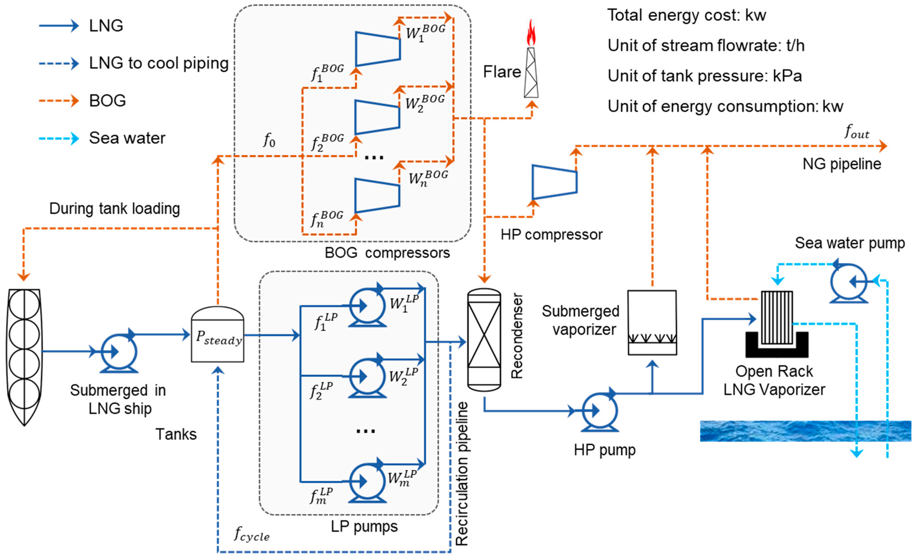
The schematic of an actual LNG terminal, which is composed of various devices, such as pumps, tanks, a recondenser, and vaporizers, is illustrated in Figure 1. As shown in Figure 1, the BOG produced in the LNG storage tanks is compressed into the recondenser with compressors, and the LNG is pumped into the recondenser by in-tank LNG pumps. When the BOG is completely condensed by the subcooled LNG in the recondenser, the BOG and the subcooled LNG are mixed into one stream. Then, the HP LNG pumps send the stream into an open rack vaporizer (ORV) or submerged vaporizer (SCV), which converts LNG to NG for commercial and household users. In some cases, the NG demands are low, and thus LNG cannot recondense all the BOG. Consequently, the HP compressors are employed to send the BOG to the NG pipes. This BOG handling process is simple, but the operating energy consumption is higher than the recondensation way [32].

This work aims to minimize the energy consumption by optimizing the recirculation flow rate and scheduling the LP pumps and BOG compressors according to natural gas demands.

As shown in Figure 1, P_steady is the steady pressure of the tank, and f₀ is the flow rate of the total BOG removed from the tank. $f_i^{BOG}$ and $W_i^{BOG}$ denote the BOG flow rate and energy consumption of compressor i, respectively. $f_j^{LP}$ and $W_j^{LP}$ denote the LNG load and energy consumption of the LP pump j, respectively. f_cycle is the flow rate of recirculating LNG. f_out is the flow rate of the output NG.

The following assumptions are made to develop the operational optimization model of the LNG terminal:

(1)

The terminal has n BOG compressors, whose load is divided into l levels;

(2)

the terminal has m fixed speed pumps, whose power consumption and flow rate load are the same;

(3)

the status of each pump or compressor is identical;

(4)

the recondensation method is used to handle BOG.

The binary variables are introduced to indicate whether the compressors or pumps are operated. Furthermore, many constraints are considered in the model.

3. Model Formulation

3.1. Basic Component Models

The models of basic components such as the storage tank, BOG compressor, LP pump, and circulating pipeline are developed as follows.

3.1.1. Tank Model

LNG storage tanks play a vital role in the terminal [37], which serve primarily as a buffer to balance the LNG supplies from ships and NG demands from local users [38]. Given the continuous heat leaking into the storage tanks, the BOG is produced inevitably [22,39]. Although the cryogenic tanks are heavily insulated from the sides and proof, external heat leakage into the LNG is unavoidable [40].

In the research of design and optimization for LNG terminals, a normal parameter is used for predicting boil-off rate generated by heat transfer from the surroundings to the tank [41]. The quantity of BOG is normally expressed as the percentage of total volume of LNG in the tank. The boil-off rate can be calculated by the following expression:

$$f=B_s\frac{V_L{\rho }_L}{24},$$

(1)

where B_s is the boil-off rate on specification ranging from 0.05%–0.1% per day [36]; V_L is the volume of LNG in tank, and ρ_L is the density of LNG.

In addition, a corrected empirical equation is widely used in recent years [28]:

$$f=\frac{C_R{B}_s{\rho }_L{V}_L}{K_1{K}_2{K}_3},$$

(2)

where the coefficient C_R is the rollover effected by the flow rate of circulating LNG, and its value is usually set as 1.2. K₁, K₂, and K₃ are the correction factors for the offset of the tank pressure (P) from the LNG vapor pressure (P_v), LNG temperature (T_L), and ambient temperature (T_a), respectively.

In this work, the HYSYS dynamic model of the LNG tank was used to generate the data of BOG generation rate varying with the operations. For convenience, the simulation data were used to regress the parameters of Equation (3), by which the total BOG generation can be calculated.

$$f={\beta }_1\left(P-P_v\right)+{\beta }_2{T}_L+{\beta }_3{T}_a+{\beta }_4,$$

(3)

where P − P_v, T_L, and T_a are the differences between the pressure of the gas phase in the tank and the vapor pressure of the LNG, the temperature of LNG, and the ambient temperature, respectively. β₁, β₂, and β₃ are the correction factors for P − P_v, T_L, and T_a, respectively. β₄ is the boil-off rate of BOG on specific conditions. The parameters can be derived from the simulation data by multi-linear regression.

3.1.2. Compressor Model

The BOG compressors are used to remove excess BOG, which may damage the infrastructure and operations of the tanks. In most LNG terminals, the optimization of compressors is the primary goal for reducing the consumption of energy, as they are highly energy intensive [26]. Industrial compressors have several types, such as reciprocating, rotary, axial, and centrifugal. In this study, the two-stage reciprocating compressors are used, and the total power consumption can be calculated as follows:

$$W^{BOG}={{\displaystyle \sum }}_{i=1}^n{W}_i^{BOG},$$

(4)

where $W_i^{BOG}$ is the power consumption of compressor i and defined as $W_i^{BOG}={{\displaystyle \sum }}_{z=0}^l{c}^z{t}_i^z$. The superscript z is the load level number of compressors, and c^z is the power consumption of level z. $t_i^z$ is the fraction of the operation period for compressor i to run at level z.

3.1.3. Pump Model

In the LNG terminal, LP pumps are used to transfer the LNG of tanks to a recondenser for cooling BOG and carry out the cold LNG to the recirculation pipeline. Therefore, the power consumption of the LP pumps is related to the send-out and recirculation flow rate. In this study, the total energy consumption (W^LP) can be calculated as follows:

$$W^{LP}={{\displaystyle \sum }}_{j=1}^m{W}_j^{LP},j=1,\cdots ,m,$$

(5)

where j is the index of pumps, and $W_j^{LP}$ is the power consumption of the LP pump j.

3.1.4. Recirculation Pipeline Model

A stream of recirculating LNG is used to keep the unloading arms in a low temperature to prevent the flow rate of the produced BOG from increasing rapidly, which may damage the devices and disturb the normal operations [22]. The heat (Q) transfers from the air to the recirculation pipeline, whose relationship with mass flow rate of recirculation pipeline is shown as follows:

$$Q=f_{cycle}{c}_p\Delta T,$$

(6)

where f_cycle is the mass flow rate of recycling LNG, c_p is the specific heat capacity, and $\Delta T=T_o-T_{in}$ is the temperature difference between inlet and outlet of recirculation pipeline. Q can also be calculated as follows:

$$Q=KA\Delta T_m,$$

(7)

$$\Delta T_m=\frac{\left(T_o-T_a\right)-\left(T_{in}-T_a\right)}{ln\frac{T_o-T_a}{T_{in}-T_a}},$$

(8)

According to Equations (6)–(8), T_o can be calculated as follows:

$$T_o=T_a-\frac{T_a-T_{in}}{e^{\frac{KA}{f^{cycle}{c}_p}}},$$

(9)

where K is the total transfer coefficient; A is the heat transfer area; T_o is the outlet temperature, and T_in is the inlet temperature of LNG.$\Delta T_m$ is log mean temperature difference.

The power consumption of LP pumps can be reduced by low f_cycle. However, low f_cycle also leads to an increase of power consumption of BOG compressors simultaneously. Therefore, f_cycle must be optimized.

3.2. Operational Optimization Model of the LNG Terminal

3.2.1. Objective Function

This work aims to obtain the optimal operation condition by minimizing the total energy consumption of the BOG compressors and LP pumps. Based on the developed basic component models, the objective function is defined as follows:

$$\begin{array}{cc}min& Energy Consumption={{\displaystyle \sum }}_{i=1}^n{W}_i^{BOG}\end{array}+{{\displaystyle \sum }}_{j=1}^m{W}_j^{LP}+\sigma {{\displaystyle \sum }}_{i=1}^n{{\displaystyle \sum }}_{z=0}^l{u}_i^z,$$

(10)

where the item ${{\displaystyle \sum }}_{i=1}^n{W}_i^{BOG}$ and ${{\displaystyle \sum }}_{j=1}^m{W}_j^{LP}$ are the electricity consumptions of compressors and LP pumps, respectively. The third one is the penalty item for the complicated operations of compressors, where σ is a small positive penalty coefficient. $u_i^z$ is the binary integer variable that indicates whether the operation mode of compressor i at level z is used. For example, using a small number of compressors is better than using several compressors. The index i and j represent the compressor and pump number, respectively, and z is the compressor load level.

3.2.2. Compressor Constraint

In order to remove the generated BOG in time, the mass flow balance for compressor i can be expressed as follows:

$${{\displaystyle \sum }}_{i=1}^n{f}_i^{BOG}=f_0,$$

(11)

$$f^z={\delta }_z{f}_{max}^{BOG},\mathrm{z}=0,\cdots ,l,$$

(12)

$$f_i^{BOG}={{\displaystyle \sum }}_{z=0}^l{\theta }_i^z{f}^z,i=1,\cdots ,n,$$

(13)

where δ_z is the load fraction at level z; $f_{max}^{BOG}$ is the mass flow rate of the compressor in the load fraction of 100%. $f^z$ is the mass flow rate of level z. The operation time constraint is given as follows:

$$x_i={{\displaystyle \sum }}_{z=0}^l{\theta }_i^z,i=1,\cdots ,n,$$

(14)

$$u_i^z\ge {\theta }_i^z,i=1,\cdots ,n,z=0,\cdots ,l,$$

(15)

where x_i is a binary integer variable indicating whether compressor i is to be used; ${\theta }_i^z$ is the fraction of the operation period for compressor i to run at level z; $u_i^z$ indicates whether the operation mode of compressor i at level z is used. The following constraint is used to avoid multiple equivalent solutions for compressors:

$$f_i^{BOG}\ge f_{i+1}^{BOG},i=1,\cdots ,n.$$

(16)

3.2.3. Pump Constraint

The total load stream supply for pumps must satisfy the stream demand of customers (f_out) when considering the mass flow of BOG and circular LNG, which can be expressed as follows:

$$f_{LNG}=f_{out}-f_0+f_{cycle},$$

(17)

$${{\displaystyle \sum }}_{j=1}^m{y}_j{f}_j^{LP}\ge f_{LNG},$$

(18)

where y_j is a binary variable that denotes whether pump j is running or not; $f_j^{LP}$ is the load of pump j, and the index j is the pump number. f_LNG is the minimum flow rate for LP pumps.

The following constraint is used to avoid multiple equivalent solutions for pumps:

$$f_j^{LP}\ge f_{j+1}^{LP},j=1,\cdots ,m.$$

(19)

3.2.4. Recirculation Pipeline Constraint

The temperature difference ($\Delta T$) between the inlet and outlet of recirculation pipeline is primarily influenced by the ambient temperature and flow rate of recirculating LNG. When the ambient temperature is fixed, the $\Delta T$ is decided by the flow rate of recirculating LNG. When the flow rate increases, the $\Delta T$ will decrease accordingly, otherwise, $\Delta T$ will increase. The temperature difference constraints of the recirculation pipeline are expressed as follows:

$$\Delta T_{min}\le \Delta T\le \Delta T_{max},$$

(20)

where $\Delta T_{min}$ and $\Delta T_{max}$ are the lower and upper bounds of $\Delta T$ [42].

The operational optimization model for the LNG terminal (LNGT-OOM) is an MINLP model, which is formally cast as follows:

$$\begin{array}{c}\underset{f^{cycle}, x_i ,u_i^z, {\theta }_i^z, y_i}{\min } Energy Consumption defined in \left(10\right)\\ s.t. Compressors constraints \left(11\right)-\left(16\right)\\ Pumps constraints \left(17\right)-\left(19\right)\\ Recirculation pipeline constraint \left(20\right)\end{array}.(\mathrm{LNGT}-\mathrm{OOM})$$

3.3. Modeling the Backup Compressors

The backup compressor must always be kept in hot standby mode to start from standby mode immediately under some sudden failures. The hot standby mode of BOG compressors also consumes energy. This operation condition is discussed in this study. Starting up a backup compressor unnecessarily is a waste of energy.

Since the load of compressors is greatly influenced by the vaporized gas of tanks, an appropriate equation of state is necessary for the sufficiently accurate description of the BOG. Considering that BOG is primarily composed of methane and nitrogen, the Soave–Redlich–Kwong (SRK) equation is used to describe the gas phase in the tank, which is calculated as follows [43,44]:

$$P=\frac{RT}{V_m-b}-\frac{a\left(T\right)}{V_m\left(V_m-b\right)},$$

(21)

$$V_m=\frac{V}{N},$$

(22)

$$b={\psi }_b\frac{R{T}_c}{P_c},$$

(23)

$$a\left(T\right)={\psi }_a\frac{{\left(R{T}_c\right)}^2}{P_c{\alpha }_T},$$

(24)

$$\alpha \left(T\right)={\left[1+k_e\left(1-T_{re}^{0.5}\right)\right]}^2,$$

(25)

$$k_e={\psi }_{k1}+{\psi }_{k2}{w}_e-{\psi }_{k3}{w}_e^2,$$

(26)

where P is the system pressure, and R is the ideal gas constant. T is the system temperature, and V_m is the molar volume. V is the system volume, and N is the moles of the system. a and b are the correction factor for intermolecular attraction and volume repulsion, respectively. w_e is the acentric factor, and the subscripts e, c, and r represent the components, critical properties, and contrast nature, respectively. α and k_e are used to make a key function of temperature and improve the accuracy of the equation [45]. Considering that the value of P changes a little with variables except for N, it can be assumed as a function of N. Among the variables, ${\gamma }_{k1}=0.48$; ψ_a = 0.42747; ψ_b = 0.08664; ψ_k1 = 0.48; ψ_k2 = 1.574, and ψ_k3 = 0.176.

The accumulation of molar flow rate (dN/dt) can be calculated as follows:

$$\frac{dN}{dt}=\frac{f-f_0}{M},$$

(27)

where f is the mass flow rate of BOG generation caused by heat leak from tanks; f₀ is the total mass load of BOG compressors; M is the molecular weight of BOG, and t is the operation time.

The operation time when moles change can be estimated as follows:

$$\Delta t=\frac{\Delta n}{\left(\frac{dN}{dt}\right)},$$

(28)

where the symbol $\Delta$ represents the differences.

If the pressure of the tank can still be kept below the flare pressure during the startup time while an operating compressor fails, then the backup compressor can be shut down during the normal operation.

4. Case Study

4.1. Case Description

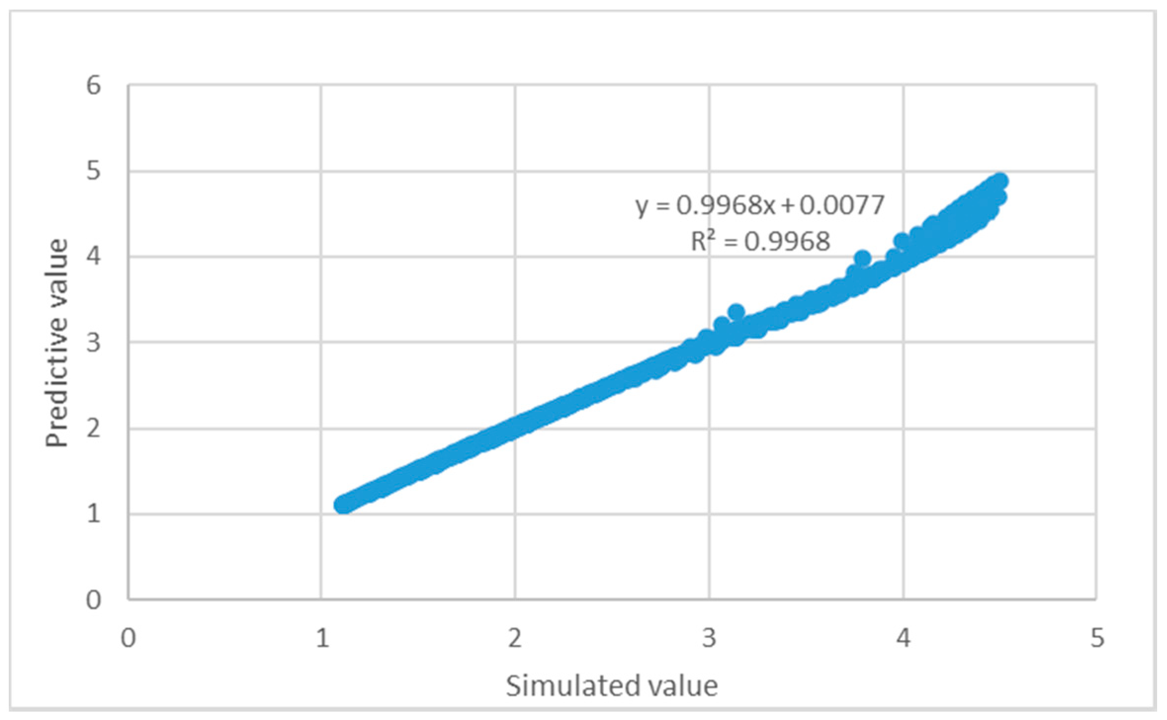
A case study on energy optimization of an actual LNG terminal in China is presented to demonstrate the effectiveness of the proposed approach. The parameters of the original condition are shown in Figure 2, and the variables and related process parameters are listed in

Table 1. Environmental variables and related process parameters of optimization.

Parameters	Values	Units
Tank number	4	/
Tank volume	16,000	m3
Tank liquid level	85	%
LNG temperature	−159.8	°C
Length of the LNG unloading pipeline	2909	m
Diameter of the LNG unloading pipeline	1.487	m
Length of the LNG cooling cycle pipeline	2942	m
Diameter of the LNG cooling cycle pipeline	0.574	m
Total heat transfer coefficient of the pipeline	0.38476	W/(m2·K)
Average ambient temperature	5	°C
Send-out flow rate	1209	t/h

.

Table 2. Regression parameters for calculating f.

Parameters	Values
β1	−0.12161
β2	−2.1252
β3	0.053183
β4	−332.666

shows the regression parameters for calculating the BOG generation rate f. Figure 3 shows the comparison between the simulated and predicted values. The average of the simulated value is 2.39 t/h, that is 0.09% for B_s (Equation (1)).

4.2. Parameters of the Proposed Models

The tanks are equipped with a cold insulation layer to ensure that the tank’s daily maximum evaporation rate does not exceed 0.1%. The flare pressure of the storage tank is 25 kPaG.

Table 3. Compositions of different types of LNG.

	Lean LNG		Rich LNG
	Mass%	Mole%	Mass%	Mole%
Methane	99.84	99.91	72.33	84.23
Ethane	0.04	0.02	20.65	12.83
Propane	0	0	6.33	2.68
i-Butane	0	0	0.31	0.1
n-Butane	0	0	0.28	0.09
Nitrogen	0.012	0.07	0.1	0.07
Total	100	100	100	100

shows the compositions of lean and rich LNG.

Table 4. Basic thermodynamic parameters of the NG components. SRK: Soave–Redlich–Kwong.

Component	Chemical Formula	Molecular Weight	SRK Acentric	Critical Temperature (°C)	Critical Pressure (kPa)
Methane	CH4	16.043	0.00740	−82.45	4641
Ethane	C2H6	30.07	0.09830	32.28	4884
Propane	C3H8	44.097	0.15320	96.75	4257
i-Butane	C4H10	58.123	0.18250	134.9	3648
n-Butane	C4H10	58.123	0.20080	152	3797
Nitrogen	N2	28.013	0.03580	−147.0	3394

lists the basic thermodynamic parameters of each component in NG.

Table 5. Binary interaction parameters of the SRK equation of state.

	Methane	Ethane	Propane	i-Butane	n-Butane	Nitrogen
Methane	/	0.00224	0.00683	0.01311	0.0123	0.03120
Ethane	0.00224	/	0.00126	0.00457	0.00410	0.03190
Propane	0.00683	0.00126	/	0.00104	0.00082	0.08860
i-Butane	0.01311	0.00457	0.00104	/	0.00001	0.13150
n-Butane	0.01230	0.00410	0.00082	0.00001	/	0.05970
Nitrogen	0.0312	0.03190	0.08860	0.13150	0.05970	/

shows the binary interaction parameters of the SRK equation of state.

As shown in Figure 2, the LNG terminal has three BOG compressors and ten LP pumps operating in the process, whose stream flow rates and power consumption are provided in

Table 6. Original operation condition of the LNG terminal.

	Variables	Original Value	Energy Consumption (kw)
Boil-off gas (BOG) compressors	x1	1	875.9
	x2	1	875.9
	x3	1	875.9
	$u_1^3$	1	/
	$u_2^3$	1	/
	$u_3^3$	1	/
BOG load (t/h)	f0	19	/
LP pumps	y1	1	210
	y2	1	210
	y3	1	210
	y4	1	210
	y5	1	210
	y6	1	210
	y7	1	210
	y8	1	210
	y9	1	210
	y10	1	210
	y11	0	0
	y12	0	0
	y13	0	0
	y14	0	0
Recirculation flow rate (t/h)	fcycle	120	/
Steady pressure (kPa)	Psteady	113.925	/
Objective function	Energy Consumption	/	4727.7

. The operating characteristics of compressors are presented in

Table 7. Operating characteristic of BOG compressors.

Property	Unit	Variable	Value
Road Levels	/	z	0	1	2	3	4
Mass load	t/h	fz	0	2.11	4.22	6.33	8.44
Load fraction	%	δ	0	25	50	75	100
Power consumptions	kw	Wc	448.3	586.2	793.1	875.9	1000
Startup time	min	$\Delta$ts	30

.

5. Results and Discussion

The flowchart of the proposed optimization modeling framework is illustrated in Figure 4. It was programmed and performed in MATLAB R2019a on a computer with an Intel I Core (TM) i9-9900 CPU @ 3.10 GHz and 32 GB RAM. The deterministic model (LNGT-OOM) was programmed in GAMS 24.1.2 and solved by the Discrete and Continuous Optimizers (DICOPT 24.1.2).

In the proposed operational optimization framework, the steady-state pressure is first presented to determine whether the results are optimal or not. Meanwhile, the SRK equation of state is selected for the physical property calculation. First, MATLAB provides the initial variables based on the actual operating condition and minimum compressor load. Additionally, then the variables are input to GAMS to obtain the optimal recirculation flow rate and number of LP pumps in operation by solving the model (LNGT-OOM). The obtained operation strategy will be sent back to MATLAB and steady-state pressure of the tank can be calculated. If the steady-state pressure is higher than the flare pressure, the compressor load must be increased, and then a new steady-state pressure is calculated. After the termination condition is achieved, whether a standby compressor needs to be turned on or not must be decided. Finally, the total power consumption of the LP pumps and BOG compressors is obtained.

The problem sizes and the computation time of the proposed MINLP model for the LNG terminal are shown in

Table 8. Problem sizes and computation time.

	Value
Number of continuous variables	57
Number of binary variables	32
Constraints	34
Number of iterations	19
Computation time (s)	0.017

.

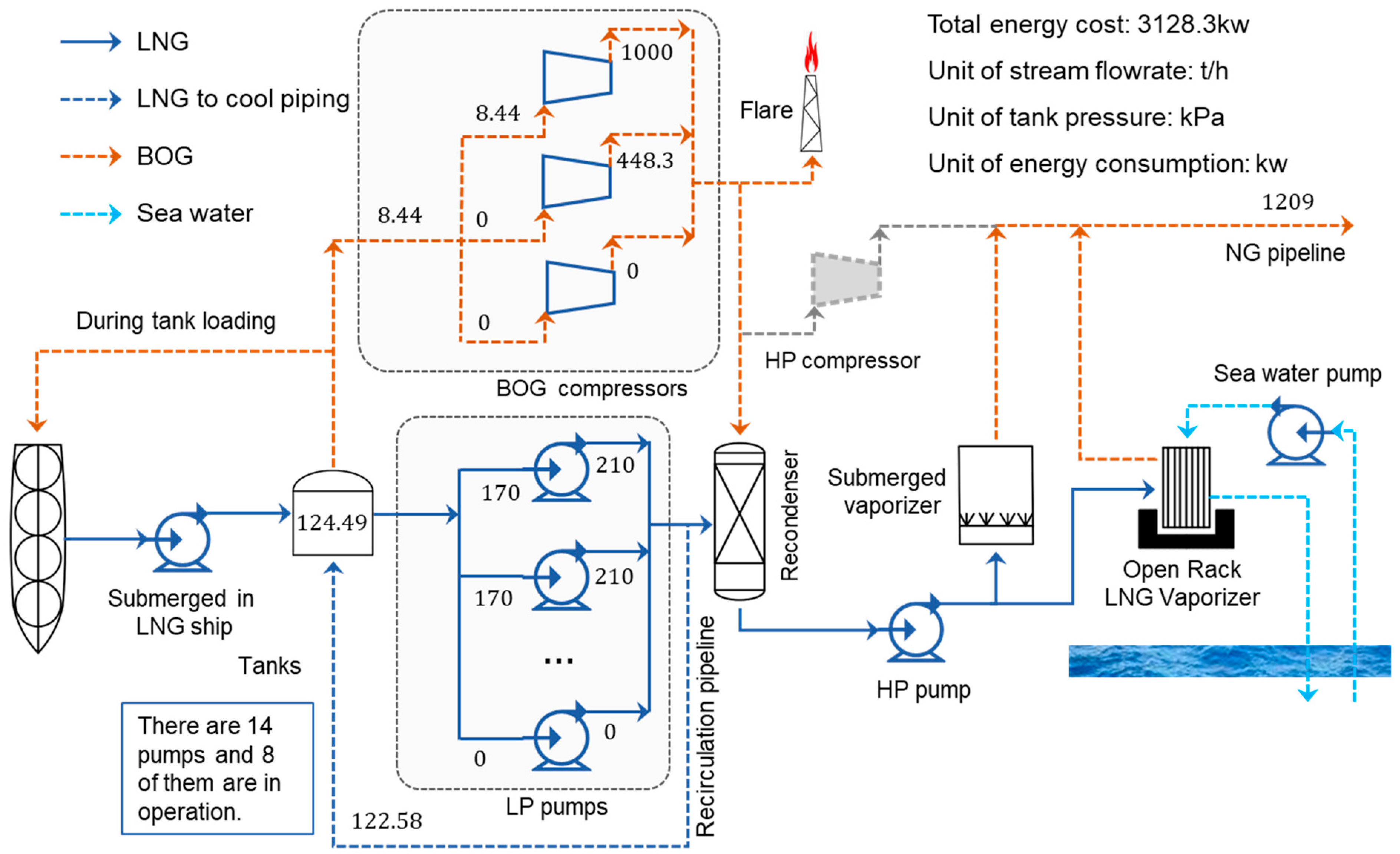
The optimized results are shown in Figure 5 and

Table 9. Optimized results and energy consumption of the model (LNGT-OOM).

	Variables	Optimized Value	Energy Consumption (kw)
BOG compressors	x1	1	1000
	x2	0	0
	x3	0	0
	$u_1^4$	1	/
	$u_2^z$	0	/
	$u_3^z$	0	/
BOG load (t/h)	f0	8.44	/
LP pumps	y1	1	210
	y2	1	210
	y3	1	210
	y4	1	210
	y5	1	210
	y6	1	210
	y7	1	210
	y8	1	210
	y9	0	0
	y10	0	0
	y11	0	0
	y12	0	0
	y13	0	0
	y14	0	0
Recirculation flow rate (t/h)	fcycle	122.58	/
Steady pressure (kPa)	Psteady	124.49	/
Objective function	Energy Consumption	/	2680

. As shown in Table 9, the total energy consumption is 2680 kw, and the steady pressure of the tank is 124.49 kPa. Two BOG compressors and two LP pumps are turned off from running. Therefore, the recirculation flow rate of LNG is increased to 122.58 t/h, and the energy consumption is reduced by 43.31%.

An operating compressor can possibly fail, therefore, the mass flow rate of BOG generation is more than the output flow rate, which leads to the accumulation of BOG and the increased pressure of the tank. The time consumed for changing from steady pressure to flare pressure ($\Delta$t_f) is 5.68 min, which can be calculated by Equation (28). It is smaller than the startup time. Therefore, a backup compressor must be turned on all the time.

The optimal operation condition is shown in Figure 6, and the energy consumption comparisons between the original and optimized operation conditions are presented in

Table 10. Energy consumption comparisons.

	Original Condition	Optimized Condition
Compressor loads (t/h)	6.33, 6.33, 6.33	8.44, 0, 0
Target pressure (kPa)	113.93	124.49
Circulation flow (t/h)	120	122.58
Pump number	10	8
Power consumption (kw)	4727.70	3128.30
Energy save (%)	/	33.83

. The energy consumption is reduced by 33.83% compared with the original condition. The energy saving results from the reduction in the number of LP pumps and the increase of the tank pressure. Moreover, the safety of the LNG tanks is ensured by the operation strategy of the backup compressors.

Furthermore, the NG demands of the end users and the ambient temperature vary all the time. Two typical scenarios in different months are implemented to indicate the effectiveness of the proposed method. The comparisons among ambient temperatures, user demands, decision variables, and optimization results for the two scenarios are summarized in

Table 11. Comparisons of data of the operating variables and results.

	April to October		November to March
	Original	Optimized	Original	Optimized
Average ambient temperature (°C)	30	30	5	5
Send-out flow rate (t/h)	555.56	555.56	1388.89	1388.89
Compressor loads (t/h)	19	14.77	19	8.44
Need a standby compressor or not	No	Yes	No	Yes
Target pressure (kPa)	113.93	122.98	113.93	124.49
Circulation flow (t/h)	120	139.21	120	122.58
Pump number	4	4	9	9
Power consumption (kw)	3467.7	3150.4	4517.7	3338.3
Energy save (%)	9.15		26.1

. For the given LNG terminal, the average ambient temperature is 30 °C, and the NG demand is 555.56 t/h from April to October. Energy consumption is reduced by 9.15%. The average ambient temperature is 5 °C, and the NG demand is 1388.89 t/h from November to March. For this scenario, 26.1% energy saving is achieved. The optimal operating variables obtained vary due to different ambient temperatures and flow rates of send-out NG.

6. Conclusions

This work proposed an operational optimization model of the LNG terminal to minimize the energy consumption of BOG compressors and LP pumps. An MINLP model was formulated, which determined whether the pumps were running or on standby, and the number of compressor level was selected as a binary variable. Operating strategies for varied flow rates of the send-out rate and the ambient temperature can be proposed using the model. An actual case study on the LNG terminal was presented to indicate the effectiveness of the proposed approach. The minimum energy consumption was determined by using the optimization model, and the corresponding decision variables were obtained.

One BOG compressor and two pumps can be turned off after optimization. The energy consumption can be reduced from 4727.70 kw to 3128.30 kw and 33.83% energy saving was obtained for the given operating condition. Furthermore, the scenarios of different months were analyzed. From April to October, when the compressor load changed from 19 t/h to 14.77 t/h and the recirculation flow rate increased from 120 t/h to 139.21 t/h, the energy consumption can be reduced by 9.15%. From November to March, the optimal operating pressure rose to 124.49 kPa due to the decrease of ambient temperatures. The optimized compressor load and recirculation flow rate were 8.44 t/h and 122.58 t/h, respectively. Compared with the previous period, 26.1% of energy can be saved after optimization. About 16.21% of energy consumption can be saved annually.

The proposed optimization method would significantly contribute to the existing LNG terminals. However, the research was on the condition that the LNG was not unloading and the LNG terminal used a recondenser instead of HP compressors to handle BOG. The other working condition will also be studied in the future. Besides, average temperatures of the months were used in this work, which is not very realistic since the ambient temperature changes all the time.

References

- He, T.; Lin, W. A novel propane pre-cooled mixed refrigerant process for coproduction of LNG and high purity ethane. Energy 2020, 202, 117784. [Google Scholar] [CrossRef]
- Arteconi, A.; Brandoni, C.; Evangelista, D.; Polonara, F. Life-cycle greenhouse gas analysis of LNG as a heavy vehicle fuel in Europe. Appl. Energy 2010, 87, 2005–2013. [Google Scholar] [CrossRef]
- Al-Haidous, S.; Al-Ansari, T. Sustainable Liquefied Natural Gas Supply Chain Management: A Review of Quantitative Models. Sustainability 2020, 12, 243. [Google Scholar] [CrossRef] [Green Version]
- Qi, M.; Park, J.; Kim, J.; Lee, I.; Moon, I. Advanced integration of LNG regasification power plant with liquid air energy storage: Enhancements in flexibility, safety, and power generation. Appl. Energy 2020, 269, 115049. [Google Scholar] [CrossRef]
- Agarwal, R.; Rainey, T.J.; Steinberg, T.; Rahman, S.M.A. LNG regasification-Effects of project stage decisions on capital expenditure and implications for gas pricing. J. Nat. Gas Sci. Eng. 2020, 78, 12. [Google Scholar] [CrossRef]
- Kurle, Y.M.; Wang, S.; Xu, Q. Dynamic simulation of LNG loading, BOG generation, and BOG recovery at LNG exporting terminals. Comput. Chem. Eng. 2017, 97, 47–58. [Google Scholar] [CrossRef]
- Wahl, P.E.; Løvseth, S.W.; Mølnvik, M.J. Optimization of a simple LNG process using sequential quadratic programming. Comput. Chem. Eng. 2013, 56, 27–36. [Google Scholar] [CrossRef] [Green Version]
- Qyyum, M.A.; Qadeer, K.; Lee, S.; Lee, M. Innovative propane-nitrogen two-phase expander refrigeration cycle for energy-efficient and low-global warming potential LNG production. Appl. Therm. Eng. 2018, 139, 157–165. [Google Scholar] [CrossRef]
- Abdul Qyyum, M.; Qadeer, K.; Lee, M. Closed-Loop Self-Cooling Recuperative N2 Expander Cycle for the Energy Efficient and Ecological Natural Gas Liquefaction Process. ACS Sustain. Chem. Eng. 2018, 6, 5021–5033. [Google Scholar] [CrossRef]
- Kumar, S.; Kwon, H.-T.; Choi, K.-H.; Lim, W.; Cho, J.H.; Tak, K.; Moon, I. LNG: An eco-friendly cryogenic fuel for sustainable development. Appl. Energy 2011, 88, 4264–4273. [Google Scholar] [CrossRef]
- He, T.; Chong, Z.R.; Zheng, J.; Ju, Y.; Ling, P. LNG cold energy utilization: Prospects and challenges. Energy 2019, 170, 557–568. [Google Scholar] [CrossRef]
- Atienza-Marquez, A.; Bruno, J.C.; Coronas, A. Cold recovery from LNG-regasification for polygeneration applications. Appl. Therm. Eng. 2018, 132, 463–478. [Google Scholar] [CrossRef]
- Lim, W.; Choi, K.; Moon, I. Current Status and Perspectives of Liquefied Natural Gas (LNG) Plant Design. Ind. Eng. Chem. Res. 2013, 52, 3065–3088. [Google Scholar] [CrossRef]
- Economides, M.J.; Wood, D.A. Natural gas and LNG trade-a global perspective. Hydrocarb Process. 2006, 85, 39–45. [Google Scholar]
- Park, C.; Lee, C.-J.; Lim, Y.; Lee, S.; Han, C. Optimization of recirculation operating in liquefied natural gas receiving terminal. J. Taiwan Inst. Chem. Eng. 2010, 41, 482–491. [Google Scholar] [CrossRef]
- Liu, C.; Zhang, J.; Xu, Q.; Gossage, J.L. Thermodynamic-Analysis-Based Design and Operation for Boil-Off Gas Flare Minimization at LNG Receiving Terminals. Ind. Eng. Chem. Res. 2010, 49, 7412–7420. [Google Scholar] [CrossRef]
- Hatcher, P.; Khalilpour, R.; Abbas, A. Optimisation of LNG mixed-refrigerant processes considering operation and design objectives. Comput. Chem. Eng. 2012, 41, 123–133. [Google Scholar] [CrossRef]
- Le, S.; Lee, J.-Y.; Chen, C.-L. Waste cold energy recovery from liquefied natural gas (LNG) regasification including pressure and thermal energy. Energy 2018, 152, 770–787. [Google Scholar] [CrossRef]
- Kanbur, B.B.; Xiang, L.; Dubey, S.; Choo, F.H.; Duan, F. Cold utilization systems of LNG: A review. Renew. Sustain. Energy Rev. 2017, 79, 1171–1188. [Google Scholar] [CrossRef]
- Lee, I.; Park, J.; You, F.; Moon, I. A novel cryogenic energy storage system with LNG direct expansion regasification: Design, energy optimization, and exergy analysis. Energy 2019, 173, 691–705. [Google Scholar] [CrossRef]
- Kochunni, S.K.; Chowdhury, K. LNG boil-off gas reliquefaction by Brayton refrigeration system–Part 1, Exergy analysis and design of the basic configuration. Energy 2019, 176, 753–764. [Google Scholar] [CrossRef]
- Rao, H.N.; Wong, K.H.; Karimi, I.A. Minimizing Power Consumption Related to BOG Reliquefaction in an LNG Regasification Terminal. Ind. Eng. Chem. Res. 2016, 55, 7431–7445. [Google Scholar] [CrossRef] [Green Version]
- Park, C.; Lim, Y.; Lee, S.; Han, C. BOG Handling Method for Energy Saving in LNG Receiving Terminal. In Computer Aided Chemical Engineering; Pistikopoulos, E.N., Georgiadis, M.C., Kokossis, A.C., Eds.; Elsevier: Amsterdam, The Netherlands, 2011; pp. 1829–1833. [Google Scholar]
- Lee, I.; Moon, I. Total Cost Optimization of a Single Mixed Refrigerant Process Based on Equipment Cost and Life Expectancy. Ind. Eng. Chem. Res. 2016, 55, 10336–10343. [Google Scholar] [CrossRef]
- Park, J.; Lee, I.; You, F.; Moon, I. Economic Process Selection of Liquefied Natural Gas Regasification: Power Generation and Energy Storage Applications. Ind. Eng. Chem. Res. 2019, 58, 4946–4956. [Google Scholar] [CrossRef]
- Reddy, H.V.; Bisen, V.S.; Rao, H.N.; Dutta, A.; Garud, S.S.; Karimi, I.A.; Farooq, S. Towards energy-efficient LNG terminals: Modeling and simulation of reciprocating compressors. Comput. Chem. Res. 2019, 128, 312–321. [Google Scholar] [CrossRef]
- Shin, M.W.; Shin, D.; Choi, S.H.; Yoon, E.S.; Han, C. Optimization of the Operation of Boil-Off Gas Compressors at a Liquified Natural Gas Gasification Plant. Ind. Eng. Chem. Res. 2007, 46, 6540–6545. [Google Scholar] [CrossRef]
- Shin, M.W.; Shin, D.; Yoon, C.E.S. Optimal operation of the boil-off gas compression process using a boil-off rate model for LNG storage tanks. Korean J. Chem. Eng. 2008, 25, 7–12. [Google Scholar] [CrossRef]
- Jang, N.; Shin, M.W.; Choi, S.H.; Yoon, E.S. Dynamic simulation and optimization of the operation of boil-off gas compressors in a liquefied natural gas gasification plant. Korean J. Chem. Eng. 2011, 28, 1166–1171. [Google Scholar] [CrossRef]
- Nagesh Rao, H.; Karimi, I.A. Optimal design of boil-off gas reliquefaction process in LNG regasification terminals. Comput. Chem. Res. 2018, 117, 171–190. [Google Scholar] [CrossRef]
- Tak, K.; Lee, I.; Kwon, H.; Kim, J. Comparison of Multistage Compression Configurations for Single Mixed Refrigerant Processes. Ind. Eng. Chem. Res. 2015, 54, 9992–10000. [Google Scholar] [CrossRef]
- Park, C.; Song, K.; Lee, S.; Lim, Y.; Han, C. Retrofit design of a boil-off gas handling process in liquefied natural gas receiving terminals. Energy 2012, 44, 69–78. [Google Scholar] [CrossRef]
- Yuan, T.; Song, C.; Junjiang, B.; Zhang, N.; Zhang, X.; He, G. Minimizing power consumption of boil off gas (BOG) recondensation process by power generation using cold energy in liquefied natural gas (LNG) regasification process. J. Clean. Prod. 2019, 238, 117949. [Google Scholar] [CrossRef]
- Wu, M.; Zhu, Z.; Sun, D.; He, J.; Tang, K.; Hu, B.; Tian, S. Optimization model and application for the recondensation process of boil-off gas in a liquefied natural gas receiving terminal. Appl. Therm. Eng. 2019, 147, 610–622. [Google Scholar] [CrossRef]
- Li, Y.; Li, Y. Dynamic optimization of the Boil-Off Gas (BOG) fluctuations at an LNG receiving terminal. J. Nat. Gas Sci. Eng. 2016, 30, 322–330. [Google Scholar] [CrossRef]
- Li, Y.; Chen, X. Dynamic simulation for improving the performance of boil-off gas recondensation system at lng receiving terminals. Chem. Eng. Commun. 2012, 199, 1251–1262. [Google Scholar] [CrossRef]
- Khan, M.S.; Effendy, S.; Karimi, I.A.; Wazwaz, A. Improving design and operation at LNG regasification terminals through a corrected storage tank model. Appl. Therm. Eng. 2019, 149, 344–353. [Google Scholar] [CrossRef]
- Trotter, I.M.; Gomes, M.F.M.; Braga, M.J.; Brochmann, B.; Lie, O.N. Optimal LNG (liquefied natural gas) regasification scheduling for import terminals with storage. Energy 2016, 105, 80–88. [Google Scholar] [CrossRef]
- Ferrín, J.L.; Pérez-Pérez, L.J. Numerical simulation of natural convection and boil-off in a small size pressurized LNG storage tank. Comput. Chem. Res. 2020, 138, 106840. [Google Scholar] [CrossRef]
- Effendy, S.; Khan, M.S.; Farooq, S.; Karimi, I.A. Dynamic modelling and optimization of an LNG storage tank in a regasification terminal with semi-analytical solutions for N2-free LNG. Comput. Chem. Res. 2017, 99, 40–50. [Google Scholar] [CrossRef]
- Dobrota, Đ.; Lalić, B.; Komar, I. Problem of Boil-off in LNG Supply Chain. Trans. Marit. Sci. 2013, 2, 91–100. [Google Scholar] [CrossRef] [Green Version]
- Lee, C.-J.; Lim, Y.; Han, C. Operational strategy to minimize operating costs in liquefied natural gas receiving terminals using dynamic simulation. Korean J. Chem. Eng. 2012, 29, 444–451. [Google Scholar] [CrossRef]
- Yuan, Z.; Cui, M.; Song, R.; Xie, Y. Evaluation of prediction models for the physical parameters in natural gas liquefaction processes. J. Nat. Gas Sci. Eng. 2015, 27, 876–886. [Google Scholar] [CrossRef]
- Ramirez-Jimenez, E.; Justo-Garcia, D.N.; Garcia-Sanchez, F.; Stateva, R.P. VLL Equilibria and Critical End Points Calculation of Nitrogen-Containing LNG Systems: Application of SRK and PC-SAFT Equations of State. Ind. Eng. Chem. Res. 2012, 51, 9409–9418. [Google Scholar] [CrossRef]
- Soave, G. Equilibrium constants from a modified Redlich-Kwong equation of state. Chem. Eng. Sci. 1972, 27, 1197–1203. [Google Scholar] [CrossRef]
Figure 1.
Structure of the liquefied natural gas (LNG) terminal with decision variables.
Figure 2.
Structure of the original condition.
Figure 3.
Comparison between simulated and predicted values.
Figure 4.
Schematic diagram of the proposed optimization framework.
Figure 5.
Optimized system configuration determined by the model (operational optimization model for the LNG terminal (LNGT-OOM)).
Figure 6.
Optimized operation condition of the proposed method.