
Estimating Breakup Frequencies in Industrial Emulsification Devices: The Challenge of Inferring Local Frequencies from Global Methods

Food Technology, Engineering and Nutrition, Lund University, SE-22100 Lund, Sweden
Processes 2021, 9(4), 645; https://0-doi-org.brum.beds.ac.uk/10.3390/pr9040645
Submission received: 12 March 2021
/
Revised: 30 March 2021
/
Accepted: 3 April 2021
/
Published: 7 April 2021
(This article belongs to the Special Issue Redesign Processes in the Age of the Fourth Industrial Revolution)
Abstract
:Experimental methods to study the breakup frequency in industrial devices are increasingly important. Since industrial production-scale devices are often inaccessible to single-drop experiments, breakup frequencies for these devices can only be studied with “global methods”; i.e., breakup frequency estimated from analyzing emulsification-experiment data. However, how much can be said about the local breakup frequencies (e.g., needed in modelling) from these global estimates? This question is discussed based on insights from a numerical validation procedure where set local frequencies are compared to global estimates. It is concluded that the global methods provide a valid estimate of local frequencies as long as the dissipation rate of turbulent kinetic energy is fairly homogenous throughout the device (although a residence-time-correction, suggested in this contribution, is needed as long as the flow is not uniform in the device). For the more realistic case of an inhomogeneous breakup frequency, the global estimate underestimates the local frequency (at the volume-averaged dissipation rate of turbulent kinetic energy). However, the relative error between local frequencies and global estimates is approximately constant when comparing between conditions. This suggest that the global methods are still valuable for studying how local breakup frequencies scale across operating conditions, geometries and fluid properties.
1. Introduction
Designing equipment and processes that allow for controlled and resource-efficient emulsification has a large relevance for chemical engineering processing. From an industrial viewpoint, most emulsification is done with high-energy-intensity methods such as high-pressure homogenizers or rotor-stator mixers. Breakup in these devices are caused by turbulent interactions between the continuous and disperse phase. Turbulent stresses first deform and elongate drops. Once critically deformed, drops break into two or more fragments [1,2,3,4,5]. A more detailed discussion on turbulent drop breakup can be found elsewhere [6,7].
From a process optimization and equipment design perspective, there is a growing interest in being able to model the evolution of the dynamic emulsion drop-size distribution from design variables [8,9,10,11,12,13]. This is often done by coupling a single phase computational fluid dynamics (CFD) simulation for modelling flow and turbulence, to a population balance equation (PBE) formulation for modelling breakup (and coalescence if applicable). Interest in using a CFD-PBE approach for model-based design and optimization is growing, in part due to the increased availability of high-performance computing. During the last couple of years there has also been an increased interest in refining these investigations both in terms of substituting the crude Reynolds averaged Navier–Stokes (RANS)-based turbulence models to large eddy simulation (LES), and in proposing new PBE solution strategies [14,15].
Regardless of which turbulence model or PBE solution strategy is employed, the PBE models need to be supplied with realistic breakup kernels to provide valid predictions. For a purely fragmenting system (such as obtained at low volume fractions of dispersed phase or high emulsifier concentration [16]), two kernels are needed: a breakup frequency (defined as the number of drops breaking per unit time) and a fragment size distribution (defined as the number of fragments formed of a certain volume from breaking a drop with a given volume). Moreover, note that a CFD-PBE approach to modelling emulsification requires that the kernels can be specified locally, for each position in the geometry. This is typically done by assuming that the local breakup frequency is controlled by the local dissipation rate of turbulent kinetic energy [11,12,13].
A large number of breakup frequency models have been suggested from theoretical considerations [17,18,19,20]. However, there is of yet no consensus on which of these that are most suitable for modelling industrially relevant breakup processes. Moreover, the turbulence found in high-pressure homogenizers, rotor-stators mixers and similar systems deviates substantially from the ideal isotropic, homogenous turbulence assumed in deriving these models [21,22,23].
Consequently, there is a need for measuring breakup frequencies, especially in industrially relevant emulsification devices. A large number of experimental method for measuring breakup frequency have been suggested (see recent review [24]). These methods can be divided in two broad classes: The first class is the “single drop breakup experiments” where an experimental model device is designed to allow optical access with high-speed photography of breaking drops. Breakup observations can then be used to, more-of-less directly, estimate a breakup frequency.
Single drop experiments can, in theory, be used to estimate the breakup frequency in each position of the device, i.e., to estimate the local breakup frequencies needed in a CFD-PBE. However, it has proved challenging to use these techniques on industrial emulsification devices. These devices often have complex geometries (e.g., the annular high-pressure homogenizer valve) or high velocities and small length-scales (e.g., breakup of µm-sized drops travelling at 100 m/s) which makes it difficult to capture breakup events with high-speed image analysis.
These difficulties have long been realized, and several methods have been suggested for estimating breakup frequencies directly from the drop-size distributions resulting from emulsification processes. This class of breakup frequency estimation methods includes three sub-classes [24]; (i) parameter fitting to PBE [9,25,26], (ii) inverse self-similarity based methods [27,28,29] and (iii) direct back-calculation methods [15,30,31].
Since the only experimental input required by these methods is the emulsion drop-size distribution, they can be applied to any emulsification device, which makes them promising for studying full-scale industrial devices. However, these emulsification-experiment based methods do, by necessity, result in a global breakup frequency, averaged across the entire emulsification device (e.g., averaged across the entire homogenizer valve in the case of high-pressure homogenization, across the whole mixer head of an inline mixer or averaged across the entire tank for a stirred batch tank), as opposed to a local breakup frequency specified at each point in the domain.
This leads to a complication for any attempt to study the breakup frequencies in industrial systems. The local breakup frequencies—which are the ones of interest for building CFD-PBE models or for testing different suggestions of theoretical breakup frequency models—are inaccessible. The globally averaged breakup frequencies can be measured. However—as will be argued in this contribution—it is not obvious what information that can be inferred about the local breakup frequency from these global estimates.
One possible research design to better understand what can be said about local frequency from global estimates would be to construct an experimental model where both classes of methods could be applied (i.e., where both single drop breakup experiments can be performed to obtain local frequencies and emulsification experiment based methods can be performed to obtain the global estimate of breakup frequency). However, such an approach has several disadvantages. Since there is yet no consensus on best practices for these methods [24], it would be difficult to separate systematic differences from experimental uncertainty. Moreover, it would be difficult to conclude on what causes the systematic differences between local and global estimates that would appear in such a comparison, if using a purely experimental approach.
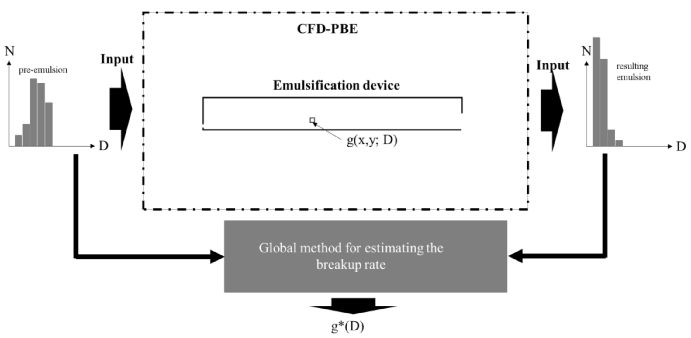
Therefore, this contribution studies the problem from a numerical perspective, by first assuming that we have a known local breakup frequency function (g(x,D) given here as a function of position x and drop diameter D), simulating what drop-size distribution this would result in, and then applying the global estimation methods to the synthetic experimental data to estimate a global average breakup frequency (g*), see illustration in Figure 1. This approach allows a direct comparison without being obscured by the experimental uncertainty. Moreover, it allows for step-wise adjusting of the simulation parameters to investigate under what conditions the global methods can be used to get useful information about the local breakup frequencies.
This study is part of an ongoing research project attempting to find methods for measuring breakup frequencies in industrial turbulent emulsification processes. The aim of this contribution is to determine under which conditions the previously suggested breakup frequency estimation methods based on emulsification data (the “global methods”) can be used to obtain quantitative information about the local frequencies.
2. Methodology
2.1. General Approach
As noted above, the objective is to investigate the relationship between the local breakup frequency and the global average as obtained from the previously suggested methods for estimating breakup frequency based on emulsification data. The general approach of the study is illustrated in Figure 1 and consists of the following steps:
- A representative geometry is chosen and the turbulent flow is modelled using single phase CFD (see Section 2.2).
- A known breakup rate, g(ε,D), is specified as a function of (equivalent sphere) drop diameter, D, and the local dissipation rate of turbulent kinetic energy, ε, together with a standard fragment size distribution, f(D,D’,ε) (see Section 2.3).
- A synthetic emulsification experiment is run using a CFD-PBE simulation with the specified breakup kernels and a well-defined initial drop-size-distribution. Information about the (steady-state) drop-size distribution exiting the device is collected (see Section 2.4).
- The global average breakup frequency is estimated using a global method from the synthetic data (i.e., using only the type of information available in an emulsification experiment on an industrial emulsification device) (see Section 2.5).
- The set local breakup frequency is compared to the global estimates.
2.2. CFD in a Model Device
2.2.1. A Representative Device Geometry
In order for the investigations to be relevant for industrial systems, the studied geometry should capture the main features of the active zone of breakup in industrial turbulent emulsification devices. The two most commonly used high energy-intensity processes are high-pressure homogenizers (low viscosity applications) and rotor-stator mixers (high viscosity applications) [32]. A high-pressure homogenizer and a rotor-stator mixer differ greatly from a macroscopic design perspective. However, the fluid flow in the breakup region is relatively similar [5]: in both cases the fluid is accelerated into a turbulent jet that interacts with a solid wall [22,33]. The jet is confined—in the case of high-pressure homogenization by the extent of the outlet chamber [34] and in the case of a rotor-stator mixer by the jets emanating from nearby slots [35]. Breakup visualizations show fragmentation occurring a few gap heights downstream in the jet where the turbulent cascade has had time to generate energetic eddies of the same length scale as the breaking drops [34,36,37] A more detailed discussion of these similarities between emulsification devices can be found elsewhere [5].
Figure 2 shows the flow-case used in this study, where fluid (density ρC = 103 kg/m3, viscosity µC = 1 mPa s) with a high uniform velocity, Ug, enters the domain through a gap of height h into a confined space. It has been set up to include the main features of the industrial devices (inhomogeneous levels of turbulence inside the device, and a flow dominated by a confined turbulent jet that interacts with a solid wall) and at the same time provide a simplified system.
Three cases with different gap velocities where modelled (see Table 1). This provides a Reynolds number range in the lower end of industrial high-pressure homogenizer and rotor-stator mixer devices [21]. (These relatively low velocities/Reynolds numbers were chosen to allow for comparisons with experimental investigations in later stage of the research project.)
2.2.2. CFD Setup
A steady-state 2D RANS-CFD was set up to model the fluid flow, using commercial CFD software (ANSYS FLUENT 12.0, Canonsburg, PA, USA). The pressure–velocity coupling was handled with a SIMPLE scheme and second order discretization was used for the transport equations.
A no-slip boundary condition was used on the walls, the inlet was assumed to have a uniform velocity equal to Ug (with a turbulence intensity of 5%) and the outlet was modelled as a pressure outlet. The realizable k-ε model [38] was used to model turbulence.
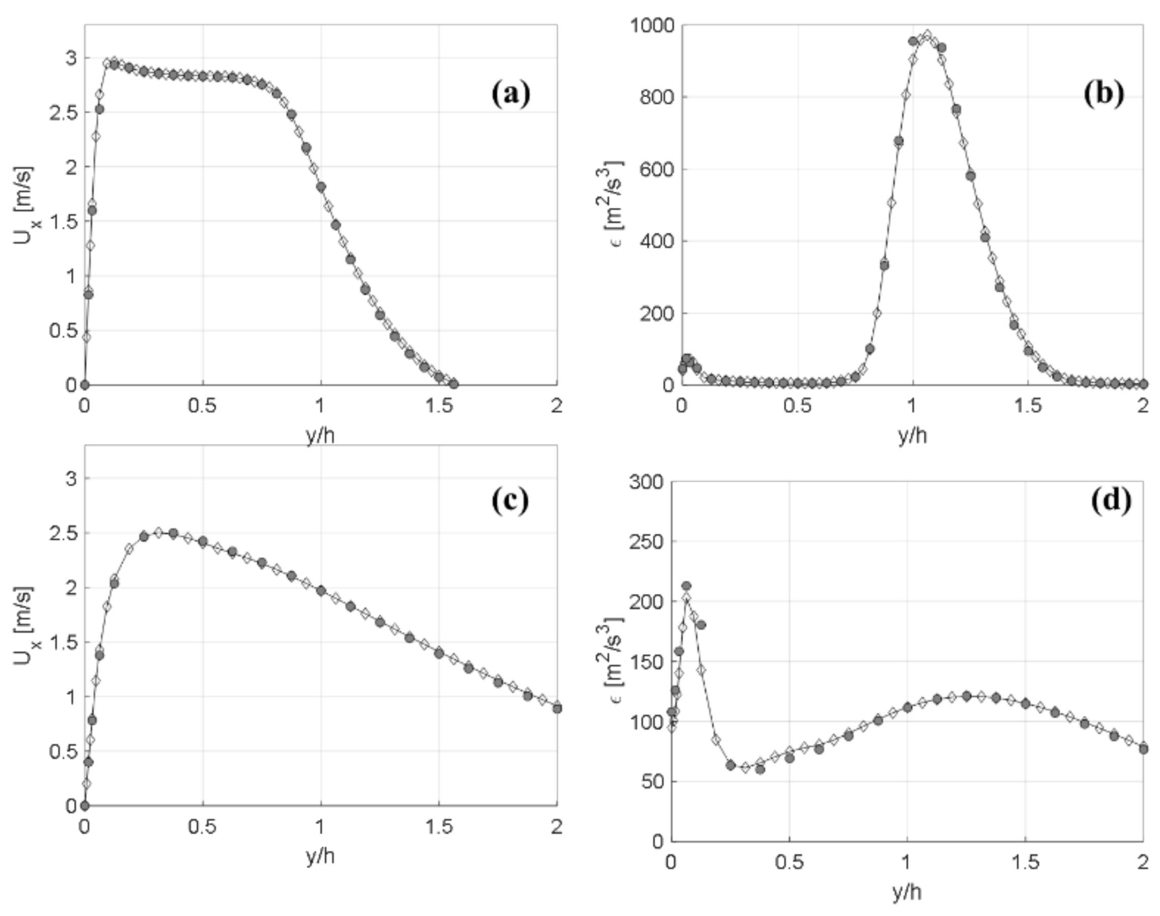
Results were generated with a mesh consisting of 18,000 cells (30 across the inlet and refined in regions of high shear and close to walls). A simulation using a lower-density mesh (73,000 cells, 50 cells across the inlet) was also run for the highest velocity (6.0 m/s), in order to test for mesh-sensitivity. Figure 3 compares the average stream-wise velocity (Ux) and dissipation rate of turbulent kinetic energy, ε, at two different lines in the flow across the two meshes (x/h = 1 and x/h = 10, see Figure 2). Since no differences can be observed, it is concluded that the mesh resolution was sufficient.
Validations with high-resolution experimental measurements of the flow-fields, both in high-pressure homogenizers [39] and rotor-stator mixers [40], have showed that RANS-CFD can accurately describe average flow and (to a lesser degree) turbulent kinetic energy (TKE) in the active region of breakup of these devices, as long as best practices are followed (realizable k-ε turbulence model, sufficient mesh resolution across the gap generating the jet, and suitable wall treatment). It should be noted that a RANS-CFD is not expected to accurately predict the details of dissipation rate of TKE in complex flows (due to general limitations in the RANS formulation [41]), and these limitations have also been confirmed in validation studies for the more specific case of emulsification devices [39,40]. However, the intention in this study is not to obtain a perfect prediction of the dissipation rate of TKE in this specific geometry but rather to obtain a reasonable and representative example of the spatial distribution of turbulence. Given that objective, the turbulence modelling is deemed sufficient.
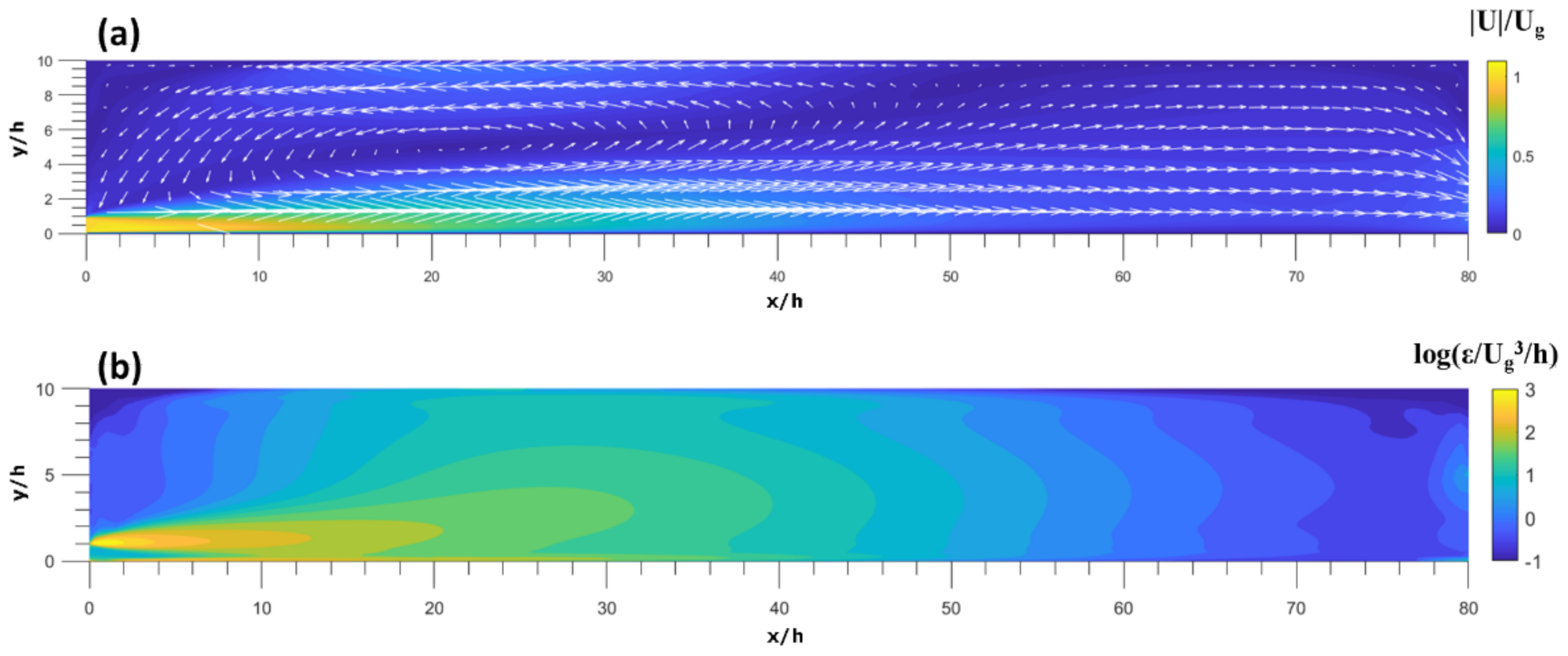
The average velocity in the device (scaled with Ug) can be seen in Figure 4a, showing the turbulent jet exiting from the gap and adhering to the lower wall. Note the characteristic recirculation zone between jet and upper confinement wall, representative of that seen for high-pressure homogenizers [34]. Figure 4b shows the spatial distribution of the dissipation rate of TKE, with high levels mainly stemming from the outer shear layers of the jet. Note that the scale is logarithmic to capture the large variations.
2.2.3. Residence Time Distributions
The residence time distribution (RTD) will be needed in obtaining a representative estimation of the global breakup frequency (see Section 2.5). This was calculated from the CFD by numerically injecting a tracer with low diffusivity (10−10 m2/s) and solving the transient transport equation (time-step 20 µs, simulations run for 2 s physical time, second-order temporal discretization) for the tracer (after which more than 99.99% of the injected tracer had exited). An extrapolation scheme was applied to describe the remaining 0.01% of the tracer, as suggested by Fogler [42]. The normalized RTD, E(t):
where c(t) is the tracer concentration exiting at time t, is displayed in Figure 5 for the three cases. The mean residence time is defined as:
2.3. Modelling Breakup
Under the assumption that no coalescence occurs (i.e., that the volume fraction of disperse phase is low), the evolution of the drop-size distribution can be modelled [43]:
where n(D;x,y) dD is the number fraction of drops of diameter in the range [D, D + dD] at position (x, y), g is the breakup frequency and f is the fragment size distribution.
As mentioned in the introduction, a large number of breakup frequency models have been suggested in the emulsification literature. These generally describe the frequency as a function of fluid properties, the equivalent sphere diameter, and the local dissipation rate of TKE. Rather than to select one of these, a general breakup frequency model with a geometric dependence on drop diameter and an exponential dependence on ε (0 < p < 1) was chosen:
This breakup model captures the approximate observed scaling breakup from single drop breakup experiments. Moreover, it has the advantage (as compared to theoretically suggested models) that it allows us to separately investigate the effect of the ε-dependency by varying p. Note that the local dissipation rate of turbulent kinetic energy has been scaled with the global average, , in Equation (4); this in order to allow for representative comparisons across cases that show different dependence on turbulence intensity.
The proportionality constant in Equation (4), C (=3.2 × 10¹²) was chosen to achieve a breakup frequency of between 10 and 150 s−1 for drop diameters between 80 and 250 µm and ε ≡ ; which would be considered reasonable breakup rates as seen from single drop breakup experiments in similar devices [44,45].
2.4. CFD-PBE to Generate Synthetic Data
The CFD was coupled to the PBE model using a built in PBE-package in the commercial software, and discretized using the fixed pivot technique [46]. The drop-size distribution was discretized into 50 classes, with a geometrical scaling ratio of 1.02, and a maximum diameter at 250 µm. The volume fraction of disperse phase was set low (0.1%) and continuous-disperse phase coupling was assumed to be one-way only (drops are assumed not to influence the turbulent flow-field and to follow the continuous phase flow perfectly); this in order to simulate the low volume fraction cases that would be of primary interest when applying the global method to estimate breakup frequency under experimental conditions.
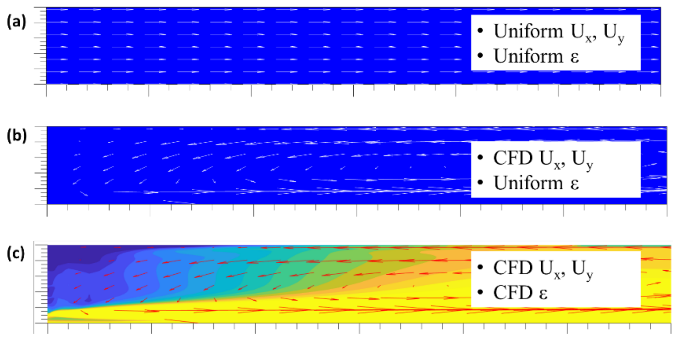
In order to study under what conditions the local (set) breakup frequency can actually be obtained by the global estimates, three different cases where set up (see illustration in Figure 6):
- Case A. Uniform flow-field and uniform ε. This case corresponds to the ideal case where all fluid elements have the same exit time from the device (i.e., an infinitely thin RTD) and where the dissipation rate of TKE (and hence the breakup frequency) is uniform throughout the entire domain. This uniform velocity is chosen so that it gives the same exit time as the mean residence time distribution at the corresponding flowrate. This is included as a validation case. For A, the global method is expected to return the local breakup frequency.
- Case B. Flow-field obtained from the CFD but with a uniform ε. This case corresponds to a device with a realistic RTD but where the variations in the turbulence intensity are so small that they are essentially uniform. This case is included to separate the effect of a uniform velocity from the effect of a uniform local breakup frequency.
- Case C. Both velocities and dissipation rate of TKE are obtained from the CFD. This corresponds to the more realistic situation in an emulsification device.
Figure 6.
Illustration of the three investigated cases. (c) represents the realistic case of an inhomogeneous velocity and turbulence, whereas (a,b) are idealized cases used to validate the method and discuss limitations.
Figure 6.
Illustration of the three investigated cases. (c) represents the realistic case of an inhomogeneous velocity and turbulence, whereas (a,b) are idealized cases used to validate the method and discuss limitations.

Each numerical experiment consisted of injecting a monodisperse size distribution with drops of either 80, 101, 128, 161, 184, 203, 218 or 250 µm diameter. The number of drops exiting the device in the different size classes were tracked (mass-weighted average across the outlet) as a function of iteration number. After 10,000 iterations, the exiting number of drops in the injected class (the data needed in estimating global rates, see Section 2.5), had converged for all studied cases, see Figure 7 for three representative example. At this point, the simulations were stopped.
2.5. Estimating Breakup Frequency from Emulsification Experiments
Several methods have been suggested for estimating the global breakup rate from emulsification experiment data (a review is available elsewhere [24]). The conceptually simplest one is to estimate the breakup frequency of the largest size class containing drops using a direct back-calculation [15,47]. If NI(t) denotes the number of drops (per unit volume) in the largest size class, I, containing drops, after having spent a time t at the globally averaged breakup frequency g*, this quantity evolves according to:
where rI,I is the redistribution factor describing how a fraction of the fragments of size between the largest and second largest class is redistributed back to class I to ensure conservation of mass and number of drops [46]:
Equation (5) is solved by:
If all drops spend the same amount of time (t = τ) in the device, the number of drops in size class I exiting the device can be obtained by NI = NI(t = τ) and the global estimate of the breakup frequency, g*, in the largest size class can be obtained directly from Equation (7):
Using Equation (8) to estimate g* will be referred to as the ‘uncorrected global estimation method’ in this study (Note that the more complex back-calculation method proposed by Vankova et al. [30] is a generalization of this approach [24]).
In the (more realistic) case where not all fluid elements spend the same amount of time in the device (the case where the RTD is not infinitely thin), non-ideal reactor theory [43,48] suggests that the average number of drops exiting the device in class I (NI) can be obtained from combining the evolution of the number of drops obtained if the exit time would be t, (NI(t)) with the scaled RTD (E(t)):
From an experimental setting (or in this case, from a synthetic experimental setting), NI/NI,0, is known, rI,I can be calculated from the set fragment size distribution and the RTD has been determined. Thus, g* can be calculated from applying a numerical equation solver to Equation (9). This will be referred to as the “RTD-corrected global estimation method” in this contribution (a simplex based method [49] in the form of the fminsearch function in MATLAB 2019b (MathWorks, Natick, MA) was used for solving Equation (9)).
3. Results and Discussion
3.1. Homogenous Flow and Breakup Frequency
Before turning to the more realistic case—where both velocity and (set) breakup frequency varies across the device geometry—the methodology was validated with the ideal case of a plug flow device where the breakup frequency is uniform (case A in Figure 6 and Section 2.4). Since the local frequency is spatially homogenous under these conditions, the global estimate should equal the set local frequency.
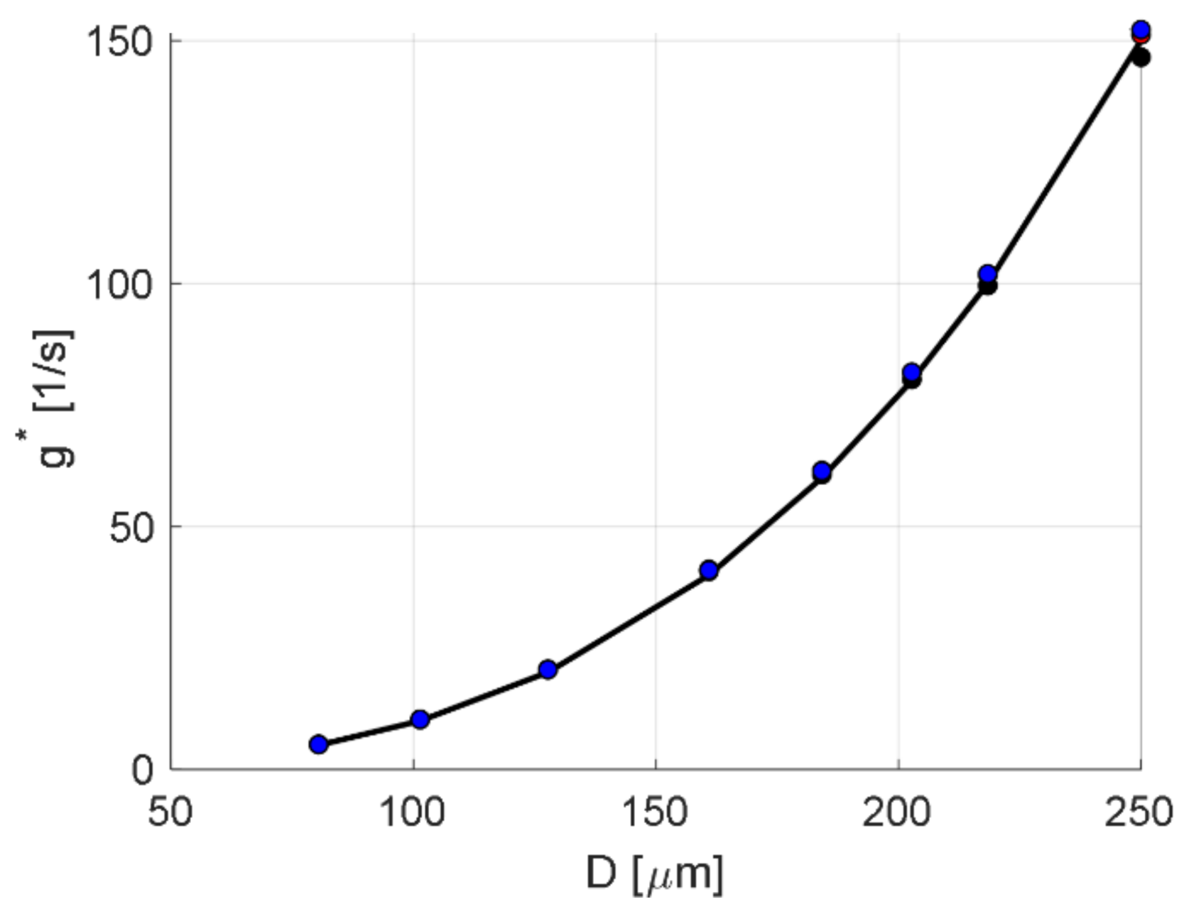
Figure 8 shows the set local breakup frequency as a function of drop diameter (solid line) with p = 1. The global estimate of the breakup frequency based on the synthetic data, and using the uncorrected method, is shown as markers (1.5 m/s in black, 3.0 m/s in red and 6.0 m/s in blue). The relative error,
can be seen in Figure 9. As seen in the figures, the estimates agree with the set values within a few percentages, regardless of jet velocity. Changing the ε-exponent (p) has no effect since the local level is forced uniformly equal to its global average (ε ≡ ), see Equation (4).
In summary, the global method (without correction) is highly suitable for estimating local breakup frequencies in the case of a homogenous flow device with a homogenous breakup frequency.
3.2. Inhomogeneous Flow and Homogenous Breakup Frequency
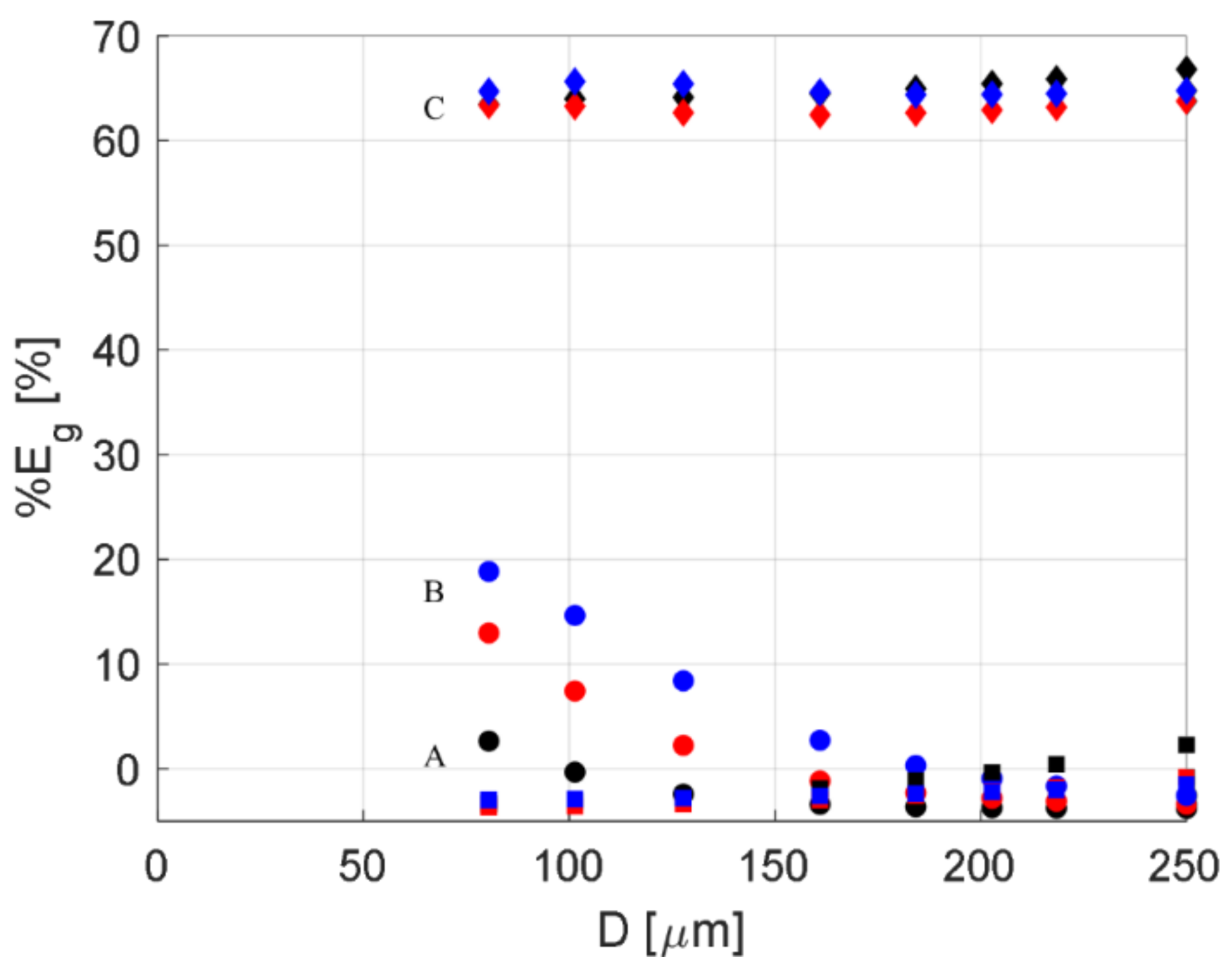
Figure 10 shows a similar comparison for the case of an inhomogeneous flow and homogenous breakup frequency (Case B in Figure 6 and Section 2.4). The circular markers show the estimates using the uncorrected global method. As seen in the figure, these misrepresents the true frequency substantially. This is expected since they assume that all drops spend the same amount of time in the device whereas the RTDs show a considerable width (see Figure 5). That the estimates are systematically underrepresenting the true frequency follows from that the peak in the RTD occurs before the mean residence time (see dashed lines in Figure 5), as is often the case for devices where a recirculation zone occurs (i.e., when the RTD has a noticeable tail).
The square markers in Figure 10 represent the RTD-corrected estimates. These show a relatively good fit to the true/set values, although the errors increase somewhat with decreasing absolute magnitudes (see Figure 9). However, this decreasing reliability of the global method is expected from an uncertainty management perspective. Since Equation (8) depends on the logarithm of the relative number of drops, it will become highly sensitive to small uncertainties if NI/NI,0 is close to one (a formal derivation and comparison between the uncertainties in Figure 9 and general uncertainty management formalism can be found in Appendix A). The consequence is that the global method (at least in the form of Equations (8) and (9)), will be less reliable under conditions where the breakup frequency is relatively low.
Thus, the global method still provides valid estimates (when corrected with the RTD), even if the device is not characterized by an ideal plug flow, as long as the local breakup frequency is homogenous throughout the device (and as long as the frequency is not very low).
3.3. Inhomogeneous Flow and Breakup Frequency
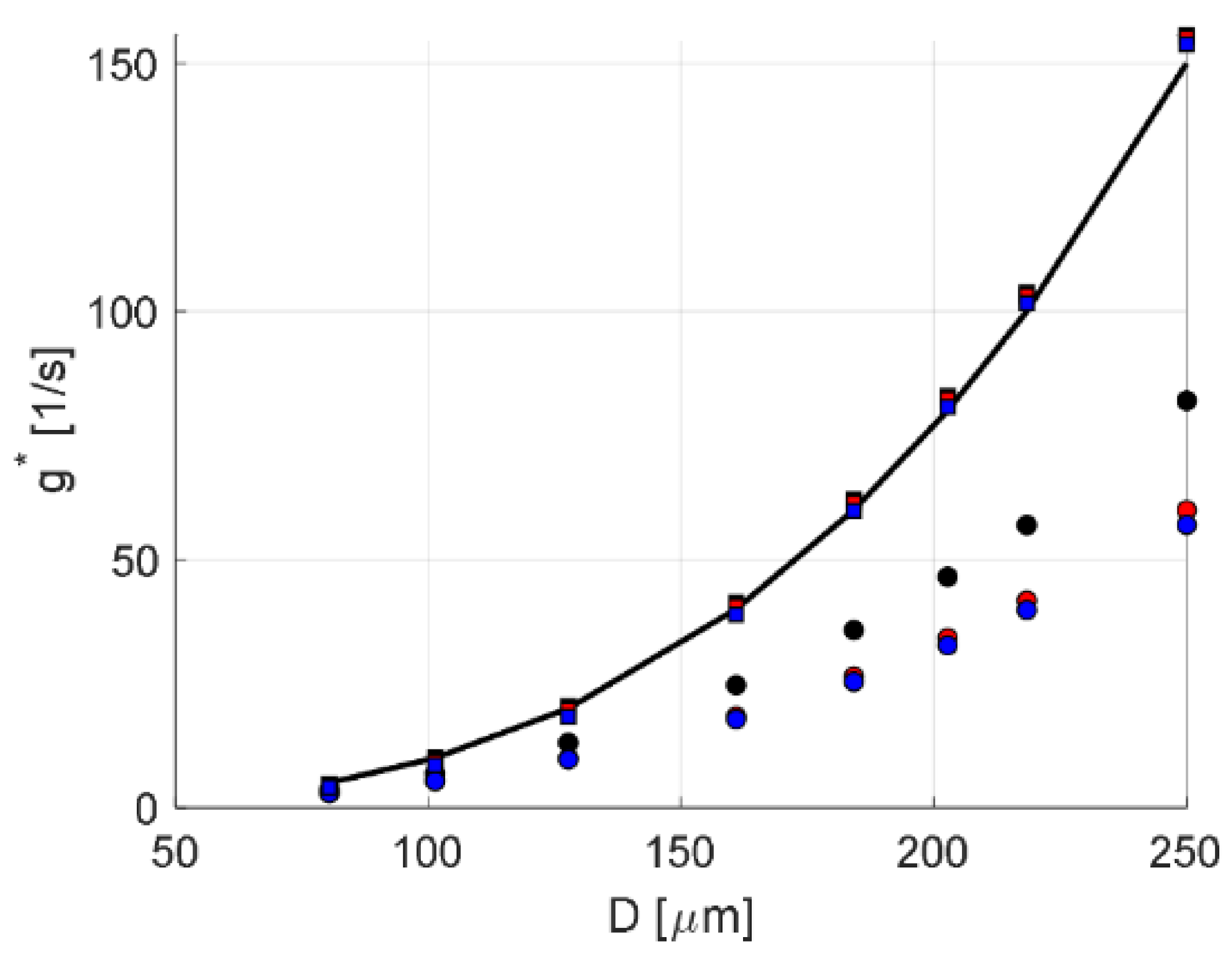
For the more realistic case of an inhomogeneous flow and breakup frequency (case C in Figure 6 and Section 2.4), it is not as clear how to make a representative comparison between local and global frequencies, since the global frequency varies spatially across the device, and the global frequency only provides one value per drop-size class. However, looking to experimental studies using these methods to discuss breakup frequency in emulsification devices (where the turbulence intensity, and hence, the breakup rate is always spatially inhomogeneous to some extent), these generally assume that the device can be characterized by a volume-averaged dissipation rate of TKE (often estimated from an energy-input-per-unit-volume argument) [25,26,29,30]. Thus, Figure 11 compares the set local breakup frequency at the volume-averaged dissipation rate of TKE in the device (obtained from the CFD) (solid line) with the global estimates, using both the uncorrected method (disk markers) and the RTD-corrected method (square markers) for the case when breakup frequency depends strongly on local dissipation rate of TKE (p = 1). The global method provides a systematic and substantial (60–70%) underestimation of the local frequency (see Figure 9). This is not unexpected, since the volume-average of the dissipation rate is not representative of what occurs in the device. As seen in Figure 4b, the local dissipation rate of TKE varies by several magnitudes across the domain, and consequently most of the breakup takes place in a narrow region inside the jet. The rest of the domain mainly transports the drop-size distribution, either towards the exit or (with a certain probability) into the recirculation zone where it will enter the jet once again and thus experience a new short period of high breakup frequency. (This behavior can also be seen from single drop experiments in industrial devices [36]).
A more representative comparison might be to compare the global average estimate to the local breakup frequency throughout the domain. Such a comparison can be seen in Figure 12. The contours show the ratio between the set local breakup frequency and the global estimate (p = 1, Ug = 3.0 m/s), with an overlay of velocity vectors representing the average flow. Note that the scaling is logarithmic to allow for a visualization of the large variation through the domain, and that local values are generally within plus/minus one order of magnitude of the global estimate.
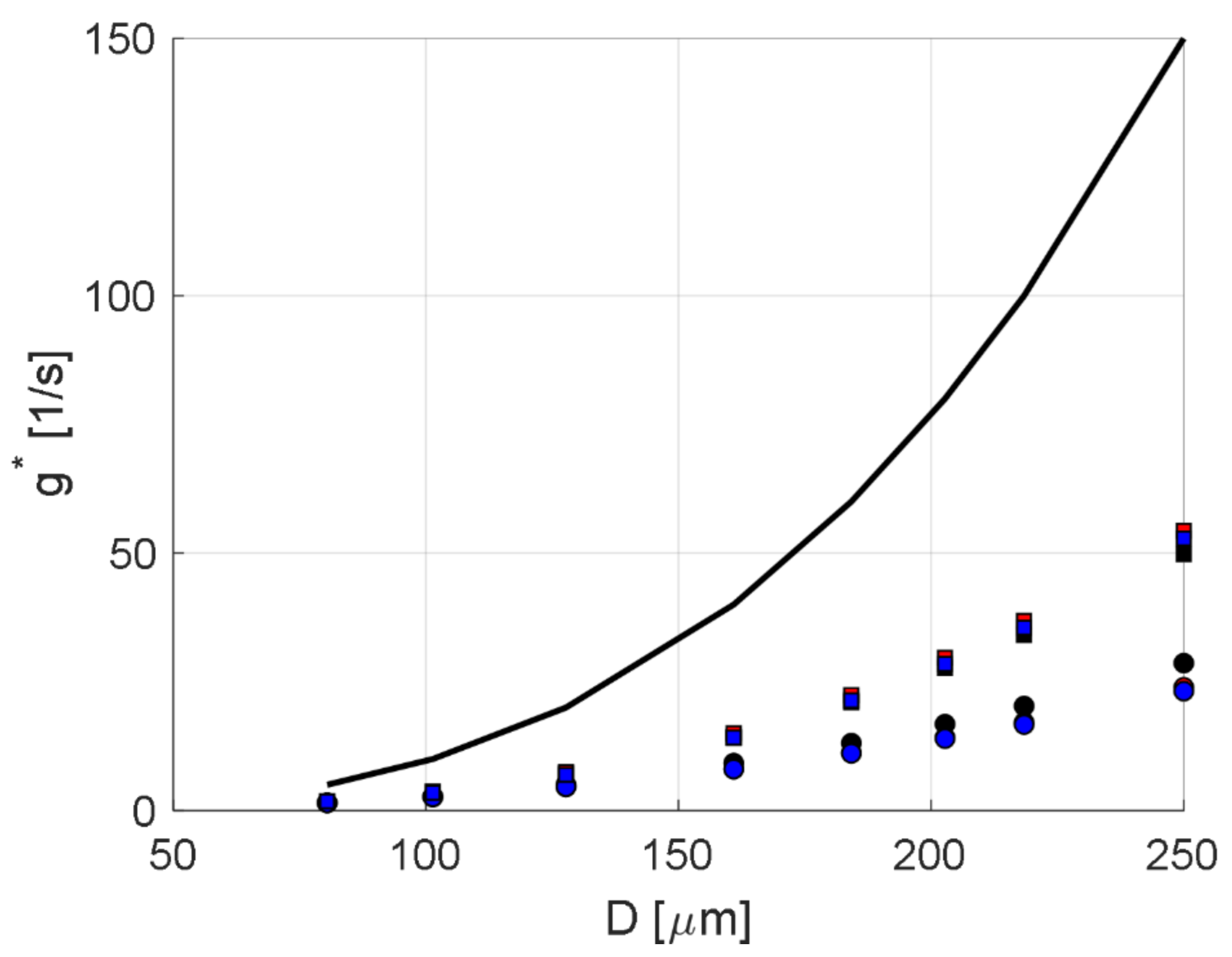
It is reasonable to expect that the deviation between global and local estimates depends on how inhomogeneous the local breakup frequency is, or alternatively put, how strong g(D,ε) depends on the local ε. Figure 11 and Figure 12 represent the case of a linear scaling (p = 1), whereas case B (Figure 9) represents the case of no dependence on local ε (p = 0). To further investigate how this deviation depends on the strength of the turbulence dependence, a range of simulations with varying p were run for inhomogeneous flow-field and turbulence. Figure 13 shows the result when the turbulence dependence is existing but weak (p = 0.01). As expected, the RTD-corrected global method now gives valid results close to those for case B.
A more extensive comparison of how the ε-dependence influences the extent of the underestimation can be seen in Figure 14. The results are showed for two jet velocities (1.5 m/s and 6.0 m/s) and for two drop diameters (representing an average breakup frequency of 10 s−1 and 150 s−1). Generally, the error increases with the scaling between breakup frequency and local breakup dissipation rate of TKE (i.e., %Eg increases with p), resulting in an underestimation of approximately 60 % for p = 1 (as was seen in Figure 9). Some variations can be seen between the different breakup frequencies and jet velocities—mainly the error is smaller when the true local breakup frequency is relatively high. However, for the investigated variations in Reynolds number (a factor 4) and in frequency (a factor 15), the underrepresentation is relatively constant, for a given value of p. This has implications for how the global methods can be used in studying industrial emulsification devices, as will be discussed further in Section 3.4.
In summary, the global method (after introducing a RTD-correction) will not return the local breakup frequency evaluated at the volume-average of the dissipation rate of TKE across the domain (unless the breakup frequency has a very weak depended on ε, i.e., unless p << 1). However, the underestimation is relatively constant across a wide range of Reynolds numbers and breakup frequency magnitudes.
3.4. The Relevance of Global Measurements
The long-term objective of this research project is to find methods for measuring breakup frequencies in industrial emulsification devices. As stated in the introduction, a large number of global (emulsification-experiment based) methods have been proposed in previous studies and these are promising in that they allow for measurements to be made on industrial devices (in contrast to the single drop breakup methods). However, global methods are also limited in that they only result in a global estimate and not in the local frequencies needed from a modelling or process optimization perspective.
The findings in this contribution show that the global methods will provide a direct and valid estimate of the local breakup frequency if the RTD-correction suggested in Section 2.5 is applied, and if the breakup frequency does not vary considerably throughout the emulsification device. This would be the case either if the turbulence intensity is highly uniform (which is rarely the case, but exceptions exist [50]), or if the breakup frequency has a weak dependence on the turbulence (p << 1). However, both theoretical suggestions and experimental single drop visualization experiments agree in suggesting a substantial ε-dependence [17,18,19,20]. As an example, Figure 15 shows the scaling proposed by Lou and Svendsens’ parameter free model [51] applied to a typical oil-in-water emulsion (ρC = 103 kg/m3, µC = 1 mPa s and interfacial tension γ = 20 mN/m) for a dissipation rate of TKE between 1 and 50 m2/s3 and drop diameters 50–500 µm. Note that the markers comply closely to a line in the loglog-plot, indicating a near constant scaling (constant p) across the ε-range. The slope varies somewhat with drop diameter but is within p = 1.3–1.4, i.e., the scaling according to this model is slightly stronger than p = 1 (cf. Figure 14).
However, in most industrially relevant turbulent emulsification devices (e.g., high-pressure homogenizers and rotor-stator mixers), the turbulence varies substantially, and thus the local breakup frequency is expected to be strongly inhomogeneous. Nevertheless, this does not necessarily imply that global estimates are without practical use. The typical research question when using one of the global methods to study breakup frequencies, is to conclude on how breakup frequency scales with operating parameters (e.g., homogenizing pressure or rotor speed), fluid properties (e.g., interfacial tension or fluid viscosity) or initial drop diameters [30,31,52]. The absolute value of the breakup frequency at a given drop volume and local dissipation rate of TKE is of less interest in these studies. As seen in Figure 14, the error is relatively constant when applied to cases with varying Reynolds number and magnitudes of breakup frequency, as long as the scaling between the local breakup frequency and the dissipation rate of TKE does not vary greatly between conditions (i.e., as long as p is constant). Moreover, as seen from Figure 15, it is not unreasonable to expect the scaling between the local breakup frequency and dissipation rate of TKE (i.e., p) to be relatively independent of drop-size under investigation. Thus, the ratio between two global breakup frequency estimations obtained by varying drop diameter, rotor speed etc. is expected to be comparable to that between the two local frequencies.
However, these comparisons should be made so that none of them gives rise to a breakup frequency that is very low in absolute terms (i.e., none of the cases should have little or no breakup, NI/NI,0 ≈ 1). As was seen in Figure 9 (and discussed in more detail in Appendix A), the global methods for estimating g* tend to amplify uncertainties in the input when NI/NI,0 is close to one.
Consequently, the global method is useful in studying how local breakup frequency scale between conditions (where both conditions give rise to substantial breakup). This scaling information could also provide a valuable input to studies attempting to suggest or validate breakup frequency models. However, some care must be taken, especially when attempting to compare small differences between conditions since neither p nor the systematic error in Figure 14 are entirely independent of operating conditions.
3.5. Limitations and Future Studies
Some limitations with the present work should be noted. First, only a single geometry was investigated whereas industrially applied emulsification devices come in different shapes and forms. The investigated geometry is not to be seen as generally applicable, but as an example of a design containing many of the features in these devices. The extent of the deviation (i.e., the magnitude of the relative errors in Figure 9), is expected to vary between geometries. Moreover, the CFD model used to generate the validation case was relatively simplistic, e.g., in using a RANS turbulence model, in assuming one-way interaction between drop and continuous phase fluid and assuming drops to follow he flow perfectly. Similarly, a specific breakup frequency model (and fragment size distribution function) is applied whereas a large number of different suggestions can be found in previous studies. The intention here was only to provide a simplistic model that allows for studying the effect of level and ε-dependence. However, the overall conclusions about under what conditions the global and local frequencies compare well (i.e., in terms of flow and dissipation rate inhomogeneity) is expected to generalize to similar devices.
As discussed in the introduction, several different methods have been suggested for estimating the global breakup frequency from an emulsification experiment [24]. Many of these methods are substantially more complex than the method discussed in Section 2.5, mainly in allowing the entire drop-diameter dependent g(D) to be estimated from a single set of emulsification experiments. Estimating more parameters from the same amount of experimental data will general reduce reliability. Thus, the relatively simple method for estimating global frequency used in this study should correspond to ideal conditions. None of the more complex methods are expected to give a more valid estimate than the method used here. In terms of reliability (i.e., how the different methods perform in propagating measurement uncertainty from inputs to the generated estimates of g*), substantially less is known [24]. The amplification of uncertainty seen from the method used in this study (Appendix A), comes from the specific form taken by Equation (8), and it is not expected to generalize to different methods.
4. Conclusions
The aim of this contribution was to determine under which conditions the previously suggested breakup frequency estimation methods based on emulsification data (the “global methods”) can be used to obtain quantitative information about the local frequencies. It can be concluded that:
- The global methods provide valid estimates of the local breakup frequencies, when the local frequencies show an insignificant spatial variation throughout the emulsification device.
- The global methods need to be supplemented with a residence-time correction to provide valid estimates, when applied to emulsification devices where the flow is not an ideal plug flow (such a correction was suggested and validated in this study).
- The global method substantially and systematically underestimates the local breakup frequency (at the volume-averaged dissipation rate of TKE) when the local breakup frequency varies spatially (e.g., due to a spatially varying turbulence intensity in the device where the breakup frequency has a substantial dependence on the dissipation rate of TKE).
- The relative error between global estimate and local frequency (at the volume-averaged dissipation rate of TKE) is constant for a relatively wide range of Reynolds numbers and break up frequency levels. This suggests that the global methods can still be used to study how local breakup frequency scale between different settings.
Funding
This research was funded by The Swedish Research Council (VR), grant number 2018-03820 and Tetra Pak Processing Systems AB.
Institutional Review Board Statement
Not applicable.
Informed Consent Statement
Not applicable.
Acknowledgments
Peyman Olad is gratefully acknowledged for providing the device geometry, scaling and CFD mesh.
Conflicts of Interest
The authors declare no conflict of interest.
Appendix A. Propagation of Uncertainty
The uncorrected method (Equation (8)) estimates the global average breakup frequency, g*, from the ratio of drops in class I after passing the device (NI) to the number originally in class I (NI,0), together with the redistribution factor (rI,I) and the average residence time (τ).
Regardless of if Equation (8) is used on experimental or numerical data, there will be some degree of uncertainty (experimental or numerical) in the inputs (mainly in the ratio X = NI/NI,0 and in τ).
If general, if an output quantity y is related to two input quantities x1 and x2 by y = f(x1, x2), the uncertainty in y, u(y), is related to the uncertainty in the inputs, u(x1) and u(x2) respectively, by: [53]
assuming x1 and x2 are uncorrelated and that each of the input uncertainties are small. By applying this general uncertainty management principle to Equation (8), one obtains:
or expressed as a relative uncertainty (i.e., by dividing Equation (A2) by the square of Equation (8)):
Equation (A3) shows that the relative uncertainty of the average residence time contributes linearly to the uncertainty in g* (or more specifically, the relative uncertainty in g* is directly proportional to the relative uncertainty of the mean residence time if X is known with certainty). However, the relationship between uncertainty in X (=NI/NI,0) and resulting uncertainty in g* is more complex. The uncertainty in the output will increase strongly as X tends towards one. This corresponds to the case where we have a low absolute breakup frequency. Thus, estimations are expected to be more uncertain the lower the absolute breakup frequency is.
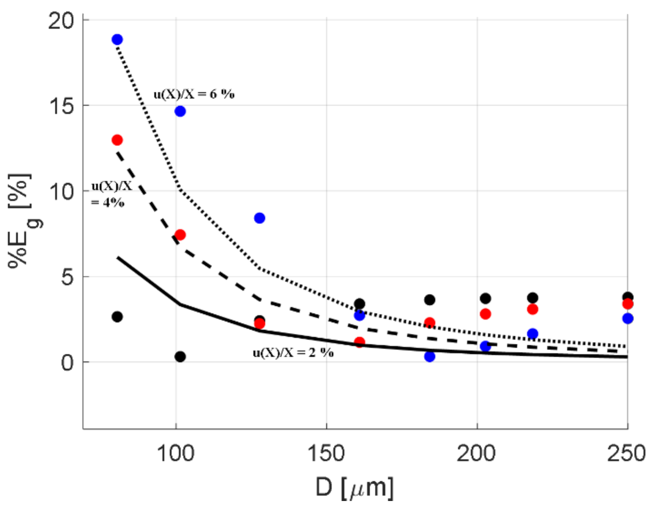
This tendency for increasing uncertainties at low breakup frequencies can also be seen when looking at the numerical results in Figure 9, where case B (homogenous breakup frequency and inhomogeneous flow) shows low deviations for large drops but a substantial deviation for small drop diameters. A comparison to the general uncertainty management framework can be seen in Figure A1, comparing the data in Figure 9 for case B, with three levels of relative uncertainty in X (2, 4 and 6%) (and assuming that τ is known with certainty).
Figure A1.
Relative error %Eg between set local breakup frequency and estimated global breakup frequency as a function of drop diameter, D for case B (markers) at three different flow conditions: Ug = 1.5 m/s (black), Ug = 3.0 m/s (red) and Ug = 6.0 m/s (blue). The results are compared to the general uncertainty management framework applied to the uncorrected method (Equation (A3)), assuming three different input uncertainties: u(X)/X = 2% (solid), 4% (dashed), 6% (dotted). Note that the uncertainty propagation turns a small uncertainty in the input (NI/NI,0) into a large uncertainty in the estimated breakup frequency when the (NI/NI,0) is relatively small (i.e., little breakup occurring).

References
- McClements, D.J.; Rao, J. Food-grade nanoemulsions: Formulation, fabrication, properties, performance, biological fate, and potential toxicity. Crit. Rev. Food Sci. Nutr. 2011, 51, 285–330. [Google Scholar] [CrossRef]
- McClements, D.J. Food Emulsions: Principles, Practices, and Techniques, 3rd ed.; CRC Press: Boca Raton, FL, USA, 2016. [Google Scholar]
- Tadros, T.; Izquierdo, P.; Esquena, J.; Solans, C. Formation and stability of nano-emulsions. Adv. Colloid Interface Sci. 2004, 108, 303–318. [Google Scholar] [CrossRef]
- Håkansson, A. Rotor-stator mixers: From batch to continuous mode of operation—A review. Processes 2018, 6, 32. [Google Scholar] [CrossRef] [Green Version]
- Håkansson, A. Emulsion formation by homogenization: Current understanding and future perspectives. Annu. Rev. Food Sci. Technol. 2019, 10, 239–258. [Google Scholar] [CrossRef] [PubMed]
- Solsvik, J.; Maass, S.; Jakobsen, H.A. Definition of a single drop breakup event. Ind. Eng. Chem. Res. 2016, 55, 2872–2882. [Google Scholar] [CrossRef]
- Mukherjee, S.; Safdari, A.; Shardt, O.; Kenjeres, S.; van den Akker, H.E.A. Droplet-turbulence interactions and quasi-equilibrium dynamics in turbulent emulsions. J. Fluid Mech. 2019, 878, 221–276. [Google Scholar] [CrossRef] [Green Version]
- Håkansson, A.; Trägårdh, C.; Bergenståhl, B. Dynamic simulation of emulsion formation in a high pressure homogenizer. Chem. Eng. Sci. 2009, 64, 2915–2925. [Google Scholar] [CrossRef]
- Raikar, N.B.; Bhatia, S.R.; Malone, M.F.; McClements, D.J.; Henson, M.A. Predicting the effect of the homogenization pressure on emulsion drop-size distributions. Ind. Eng. Chem. Res. 2011, 50, 6089–6100. [Google Scholar] [CrossRef]
- Becker, P.J.; Puel, F.; Jakobsen, H.A.; Sheibat-Othman, N. Development of and improved breakage kernel for high dispersed viscosity phase emulsification. Chem. Eng. Sci. 2014, 109, 326–338. [Google Scholar] [CrossRef]
- Janssen, J.J.M.; Hoogland, H. Modelling strategies for emulsification in industrial practice. Can. J. Chem. Eng. 2014, 92, 198–202. [Google Scholar] [CrossRef]
- Maindarkar, S.N.; Hoogland, H.; Hansen, M.A. Predicting the combined effects of oil and surfactant concentrations on the drop size distributions of homogenized emulsions. Colloids Surf. A Physicochem. Eng. Asp. 2015, 467, 18–30. [Google Scholar] [CrossRef]
- Guan, X.; Yang, N.; Nigam, K. Prediction of droplet size distribution for high pressure homogenizer with heterogeneous turbulent dissipation rate. Ind. Eng. Chem. Res. 2020, 59, 4020–4032. [Google Scholar] [CrossRef]
- Salehi, F.; Cleary, M.J.; Masri, A.R. Population balance equation for turbulent polydisperse inertial droplets and particles. J. Fluid Mech. 2017, 831, 719–742. [Google Scholar] [CrossRef]
- Aiyer, A.K.; Yang, D.; Chamecki, M.; Meneveau, C. A population balance model for large eddy simulation of polydisperse droplet evolution. J. Fluid Mech. 2019, 878, 700–739. [Google Scholar] [CrossRef] [Green Version]
- Jafari, S.M.; Assadpoor, E.; He, Y.; Bhandari, B. Re-coalescence of emulsion droplets during high-energy emulsification. Food Hydrocoll. 2008, 22, 1191–1202. [Google Scholar] [CrossRef]
- Liao, Y.; Lucas, D. A literature review of theoretical models for drop and bubble breakup in turbulent dispersions. Chem. Eng. Sci. 2009, 64, 3389–3406. [Google Scholar] [CrossRef]
- Lasheras, J.C.; Eastwood, C.; Martínez-Bazán, C.; Montañés, J.L. A review of statistical models for the break-up of an immiscible fluid immersed into a fully developed turbulent flow. Int. J. Multiph. Flow 2002, 28, 247–278. [Google Scholar] [CrossRef] [Green Version]
- Sajjadi, B.; Raman, A.A.A.; Shah, R.S.S.R.E.; Ibrahim, S. Review on applicable breakup/coalescence models in turbulent liquid-liquid flows. Rev. Chem. Eng. 2013, 29, 131–158. [Google Scholar] [CrossRef]
- Solsvik, J.; Tangen, S.; Jakobsen, H.A. On the constitutive equations for fluid particle breakage. Rev. Chem. Eng. 2013, 29, 241–356. [Google Scholar] [CrossRef]
- Håkansson, A. Scale-down failed—Dissimilarities between high-pressure homogenizers of different scales due to failed mechanistic matching. J. Food Eng. 2017, 195, 31–39. [Google Scholar] [CrossRef]
- Håkansson, A.; Fuchs, L.; Innings, F.; Revstedt, J.; Trägårdh, C.; Bergenståhl, B. High resolution experimental measurement of turbulent flow field in a high pressure homogenizer model its implication on turbulent drop fragmentation. Chem. Eng. Sci. 2011, 66, 1790–1801. [Google Scholar] [CrossRef]
- Bagkeris, I.; Michel, V.; Prosser, R.; Kowalski, A. Large-eddy simulation in a Sonolator high-pressure homogeniser. Chem. Eng. Sci. 2020, 215, 115441. [Google Scholar] [CrossRef]
- Håkansson, A. Experimental methods for measuring the breakup frequency in turbulent emulsification: A critical review. Chem. Eng. Sci. 2020, 4, 52. [Google Scholar] [CrossRef]
- Coulaloglou, C.A.; Tavlarides, L.L. Description of interaction processes in agitated liquid-liquid dispersions. Chem. Eng. Sci. 1977, 32, 1289–1297. [Google Scholar] [CrossRef]
- Ribeiro, M.M.; Regueiras, P.F.; Guimaraes, M.M.L.; Madureira, C.M.N.; Cruz-Pinto, J.J.C. Optimization of breakage and coalescence model parameters in a steady-state batch agitated dispersion. Ind. Eng. Chem. Res. 2011, 50, 2182–2191. [Google Scholar] [CrossRef]
- Sathyagal, A.N.; Ramkrishna, D.; Narsimhan, G. Solution of inverse problems in population balances—II. Particle break-up. Comput. Chem. Eng. 1995, 19, 437–451. [Google Scholar] [CrossRef]
- Kostoglou, M.; Karabelas, A.J. A contribution towards predicting the evolution of droplet size distribution in flowing dilute liquid/liquid dispersions. Chem. Eng. Sci. 2001, 56, 4283–4292. [Google Scholar] [CrossRef]
- O’Rourke, A.M.; MacLoughlin, P.F. A study of drop breakup in lean dispersions using the inverse-problem method. Chem. Eng. Sci. 2010, 65, 3681–3694. [Google Scholar] [CrossRef]
- Vankova, N.; Tcholakova, S.; Denkov, N.D.; Vulchev, V.D.; Danner, T. Emulsification in turbulent flow 2. Breakage rate constants. J. Colloid Interface Sci. 2007, 313, 612–629. [Google Scholar] [CrossRef]
- Hounslow, M.J.; Ni, X. Population balance modelling of droplet coalescence and break-up in an oscillatory baffled reactor. Chem. Eng. Sci. 2004, 59, 819–828. [Google Scholar] [CrossRef]
- Schultz, S.; Wagner, G.; Urban, K.; Ulrich, J. High-pressure homogenization as a process for emulsification. Chem. Eng. Technol. 2004, 27, 361–368. [Google Scholar] [CrossRef]
- Mortensen, H.H.; Calabrese, R.V.; Innings, F.; Rosendahl, L. Characteristics of a batch rotor-stator mixer performance elucidated by shaft torque and angle resolved PIV measurements. Can. J. Chem. Eng. 2011, 89, 1076–1095. [Google Scholar] [CrossRef]
- Innings, F.; Trägårdh, C. Visualization of the drop deformation and break-up process in a high pressure homogenizer. Chem. Eng. Technol. 2005, 28, 882–891. [Google Scholar] [CrossRef]
- Mortensen, H.H.; Innings, F.; Håkansson, A. The effect of stator design on flowrate and velocity fields in a rotor-stator mixer—An experimental investigation. Chem. Eng. Res. Des. 2017, 121, 245–254. [Google Scholar] [CrossRef]
- Ashar, M.; Arlov, D.; Carlsson, F.; Innings, F.; Andersson, R. Single droplet breakup in a rotor-stator mixer. Chem. Eng. Sci. 2018, 181, 186–198. [Google Scholar] [CrossRef]
- Kelemen, K.; Gepperth, S.; Koch, R.; Bauer, H.-J.; Schuchmann, H.P. On the visualization of droplet deformation and breakup during high-pressure homogenization. Microfluid. Nanofluid. 2015, 19, 1139–1158. [Google Scholar] [CrossRef]
- Shih, T.-H.; Liou, W.W.; Shabbir, A.; Yang, Z.; Zhu, J. A new k-ε eddy viscosity model for high Reynolds number turbulent flows. Comput. Fluids 1995, 24, 227–238. [Google Scholar] [CrossRef]
- Håkansson, A.; Fuchs, L.; Innings, F.; Revstedt, J.; Trägårdh, C.; Bergenståhl, B. Experimental validation of k–ε RANS-CFD on a high-pressure homogenizer valve. Chem. Eng. Sci. 2012, 71, 264–273. [Google Scholar] [CrossRef]
- Mortensen, H.H.; Arlov, D.; Innings, F.; Håkansson, A. A validation of commonly used CFD methods applied to Rotor Stator Mixers using PIV measurements of fluid velocity and turbulence. Chem. Eng. Sci. 2018, 177, 340–353. [Google Scholar] [CrossRef]
- Pope, S.B. Turbulent Flows; Cambridge University Press: Cambridge, UK, 2000. [Google Scholar]
- Fogler, S.H. Chapter 16. Residence time distributions of chemical reactors. In Elements of Reactor Engineering, 5th ed.; Fogler, S.H., Ed.; Pearson Education: London, UK, 2016; pp. 767–806. [Google Scholar]
- Ramkrishna, D. Population Balances—Theory and Applications to Particulate Systems in Engineering; Academic Press: San Diego, CA, USA, 2000. [Google Scholar]
- Maaß, S.; Kraume, M. Determination of breakage rates using single drop experiments. Chem. Eng. Sci. 2012, 70, 146–164. [Google Scholar] [CrossRef]
- Vejražka, J.; Zedníková, M.; Stranovský, P. Experiments on breakup of bubbles in a turbulent flow. AIChE J. 2018, 64, 740–757. [Google Scholar] [CrossRef]
- Kumar, S.; Ramkrishna, D. On the solution of population balance equations by discretization—I. A fixed pivot technique. Chem. Eng. Sci. 1996, 51, 1311–1332. [Google Scholar] [CrossRef]
- Martínez-Bazán, C.; Montañés, J.L.; Lasheras, J.C. On the breakup of an air bubble injected into a fully developed turbulent flow. Part 1. Breakup frequency. J. Fluid Mech. 1999, 401, 157–182. [Google Scholar] [CrossRef] [Green Version]
- Zwietering, T.N. The degree of mixing in continuous flow systems. Chem. Eng. Sci. 1959, 11, 1–15. [Google Scholar] [CrossRef]
- Lagarias, J.C.; Reeds, J.A.; Wright, M.H.; Wright, P.E. Convergence properties of the Nelder-Mead simplex method in low dimensions. SIAM J. Optim. 1998, 9, 112–147. [Google Scholar] [CrossRef] [Green Version]
- Bouaifi, M.; Mortensen, M.; Andersson, R.; Orciuch, W.; Andersson, B.; Chopard, F.; Norén, T. Experimental and numerical investigations of a jet mixing in a multifunctional channel reactor. Passive and reactive systems. Chem. Eng. Res. Des. 2004, 82, 274–283. [Google Scholar] [CrossRef]
- Luo, H.; Svendsen, H.F. Theoretical model for drop and bubble breakup in turbulent dispersions. AIChE J. 1996, 42, 1225–1233. [Google Scholar] [CrossRef]
- Sathyagal, A.N.; Ramkrishna, D. Droplet breakage in stirred dispersions. Breakage functions from experimental drop-size distributions. Chem. Eng. Sci. 1996, 51, 1377–1391. [Google Scholar] [CrossRef]
- Evaluation of Measurement Data—Guide to the Expression of Uncertainty in Measurements (JCGM 100:2008). Available online: https://www.bipm.org/en/publications/guides/gum.html (accessed on 25 March 2021).
Figure 1.
Schematic representation of the difference between local breakup frequency in point (x,y) for drop diameters D, g(x,y;D), and the global estimate, g*(D), and illustrating the research approach, see Section 2.
Figure 1.
Schematic representation of the difference between local breakup frequency in point (x,y) for drop diameters D, g(x,y;D), and the global estimate, g*(D), and illustrating the research approach, see Section 2.

Figure 2.
The flow-case investigated in this study, chosen to capture the main features of the confined turbulent wall-jet in which drop breakup takes place in high-pressure homogenizers and rotor-stator mixers. Dashed vertical lines show the location of x/h = 1 and x/h = 10.
Figure 2.
The flow-case investigated in this study, chosen to capture the main features of the confined turbulent wall-jet in which drop breakup takes place in high-pressure homogenizers and rotor-stator mixers. Dashed vertical lines show the location of x/h = 1 and x/h = 10.

Figure 3.
Mesh resolution validation. (a,c): Stream-wise average velocity, Ux, and (b,d): dissipation rate of TKE, ε, on two lines perpendicular to the lower wall (x/h = 1 in (a,b) and at x/h = 10 in (c,d)). Grey markers show the mesh used in the study, the white markers show the denser mesh used in the mesh-validation stage only.

Figure 4.
(a) Average velocity, |U|, and (b) dissipation rate of TKE, ε, in the flow geometry, scaled with gap velocity, Ug, and gap height, h. (Ug = 3.0 m/s). Note the logarithmic scale in B.
Figure 4.
(a) Average velocity, |U|, and (b) dissipation rate of TKE, ε, in the flow geometry, scaled with gap velocity, Ug, and gap height, h. (Ug = 3.0 m/s). Note the logarithmic scale in B.

Figure 5.
Dimensionless residence time distributions, E(t), for the three cases, Ug = 1.5 m/s (black), 3.0 m/s (red) and 6.0 m/s (blue). Dashed lines show the mean residence time for the three cases respectively.
Figure 5.
Dimensionless residence time distributions, E(t), for the three cases, Ug = 1.5 m/s (black), 3.0 m/s (red) and 6.0 m/s (blue). Dashed lines show the mean residence time for the three cases respectively.

Figure 7.
Convergence history of the exiting number of drops normalized to the entering number of drops in the injection size-class (NI/NI,0), showing three representative examples.
Figure 7.
Convergence history of the exiting number of drops normalized to the entering number of drops in the injection size-class (NI/NI,0), showing three representative examples.

Figure 8.
Case A: Homogenous flow and breakup frequency. Set breakup frequency (line) compared to global estimate (markers) at different drop diameters, D. Results from three flow conditions: Ug = 1.5 m/s (black), Ug = 3.0 m/s (red) and Ug = 6.0 m/s (blue).
Figure 8.
Case A: Homogenous flow and breakup frequency. Set breakup frequency (line) compared to global estimate (markers) at different drop diameters, D. Results from three flow conditions: Ug = 1.5 m/s (black), Ug = 3.0 m/s (red) and Ug = 6.0 m/s (blue).

Figure 9.
Relative error %Eg between set local breakup frequency and estimated global breakup frequency as a function of drop diameter, D. Results are showed for the three cases: A (squares), B (disks) and C (diamonds) in Figure 6 and for three different flow conditions: Ug = 1.5 m/s (black), Ug = 3.0 m/s (red) and Ug = 6.0 m/s (blue).

Figure 10.
Case B: Inhomogeneous flow but homogenous breakup frequency. Set breakup frequency (line) compared to global estimate (circles: uncorrected, squares: RTD-corrected) at different drop diameters, D. Results from three flow conditions: Ug = 1.5 m/s (black), Ug = 3.0 m/s (red) and Ug = 6.0 m/s (blue).

Figure 11.
Case C: Inhomogeneous flow and breakup frequency (p = 1). Set breakup frequency (line) compared to global estimate (circles: uncorrected, squares: RTD-corrected)) at different drop diameters, D. Results from three flow conditions: Ug = 1.5 m/s (black), Ug = 3.0 m/s (red) and Ug = 6.0 m/s (blue).

Figure 12.
Comparison between the local breakup frequency (g) and the global estimate (g*). Note the logarithmic scaling. Vectors represent average velocity. (p = 1, Ug = 3.0 m/s).
Figure 12.
Comparison between the local breakup frequency (g) and the global estimate (g*). Note the logarithmic scaling. Vectors represent average velocity. (p = 1, Ug = 3.0 m/s).

Figure 13.
Case C: Inhomogeneous flow and breakup frequency (p = 0.01). Set breakup frequency (line) compared to global estimate (square: RTD-corrected) at different drop diameters, D. Results from two flow conditions: Ug = 1.5 m/s (black) and Ug = 6.0 m/s (blue).
Figure 13.
Case C: Inhomogeneous flow and breakup frequency (p = 0.01). Set breakup frequency (line) compared to global estimate (square: RTD-corrected) at different drop diameters, D. Results from two flow conditions: Ug = 1.5 m/s (black) and Ug = 6.0 m/s (blue).

Figure 14.
The relative error between global estimate and local breakup frequency, %Eg, as a function 1.5 m/s, black, and 6.0 m/s, blue) and two breakup frequency levels (10 s−1 and 150 s−1).
Figure 14.
The relative error between global estimate and local breakup frequency, %Eg, as a function 1.5 m/s, black, and 6.0 m/s, blue) and two breakup frequency levels (10 s−1 and 150 s−1).

Figure 15.
Scaling between local breakup frequency, g, and dissipation rate of TKE, ε, according to the model suggested by Lou and Svendsen for an oil-in-water emulsion (ρC = 103 kg/m3, µC = 1 mPa s, γ = 20 mN/m) with drop diameters between 50 and 500 µm. The dash-dotted red line shows the scaling g ~ εp with p = 1 as a comparison.


Table 1.
Flow settings in the model device compared to industrial high-pressure homogenizers (HPHs) and rotor-stator mixers (RSMs).
Publisher’s Note: MDPI stays neutral with regard to jurisdictional claims in published maps and institutional affiliations. |
© 2021 by the author. Licensee MDPI, Basel, Switzerland. This article is an open access article distributed under the terms and conditions of the Creative Commons Attribution (CC BY) license (https://creativecommons.org/licenses/by/4.0/).
Share and Cite
MDPI and ACS Style
Håkansson, A. Estimating Breakup Frequencies in Industrial Emulsification Devices: The Challenge of Inferring Local Frequencies from Global Methods. Processes 2021, 9, 645. https://0-doi-org.brum.beds.ac.uk/10.3390/pr9040645
AMA Style
Håkansson A. Estimating Breakup Frequencies in Industrial Emulsification Devices: The Challenge of Inferring Local Frequencies from Global Methods. Processes. 2021; 9(4):645. https://0-doi-org.brum.beds.ac.uk/10.3390/pr9040645
Chicago/Turabian StyleHåkansson, Andreas. 2021. "Estimating Breakup Frequencies in Industrial Emulsification Devices: The Challenge of Inferring Local Frequencies from Global Methods" Processes 9, no. 4: 645. https://0-doi-org.brum.beds.ac.uk/10.3390/pr9040645
Note that from the first issue of 2016, this journal uses article numbers instead of page numbers. See further details here.