Study on Hull Optimization Process Considering Operational Efficiency in Waves

Abstract

This study investigates the optimization of the hull form of a tanker, considering the operational efficiency in waves, in accordance with the recent Energy Efficiency Design Index regulation. For this purpose, the total resistance and speed loss of the ship under representative sea conditions were minimized simultaneously. The total resistance was divided into three components: calm water resistance, added resistance due to wind, and to waves. The first two components were calculated using regression formulas, and the last component was estimated using the strip theory, far-field method, and the short-wave correction formula. Next, prismatic coefficient, waterline length, waterplane area, and flare angle were selected as design variables from the perspective of operational efficiency. The hull form was described as a combination of cross-sectional curves. A combination of the method shifting these sections in the longitudinal direction and the Free-Form Deformation method was used to deform the hull. As a result of applying the non-dominated sorting genetic algorithm to a tanker, the hull was deformed thinner and longer, and it was determined that the total resistance and speed loss were reduced by 3.58 and 10.2%, respectively. In particular, the added resistance due to waves decreased significantly compared to the calm water resistance, which implies that the present tendency differs from conventional ship design that optimizes only the calm water resistance.

1. Introduction

In ship design procedures, a complex and systematic optimization process is needed that considers the combination of functions to be optimized, disciplines to be considered, and requirements of stakeholders. Traditionally, the ship design forms part of the life cycle of a ship that can be divided into five stages, as suggested by Papanikolaou [1]: concept/preliminary design, contractual and detailed design, ship construction/fabrication process, ship operation for economic life, and scrapping/recycling. In line with the fourth stage (ship operation for economic life), hull form optimization using various numerical analysis tools has been carried out since the 1960s to reduce ship resistance as computing power has improved. Weinblum [2] introduced mathematical theories on minimizing resistance from a ship design perspective and attempted to reduce the gap between practical shipbuilders and theoretical researchers. Dawson [3] developed the modified Rankine source method to apply to the wave resistance problem, which was later applied to several studies on ship design that minimized wave resistance. In addition, numerous computer-aided studies have optimized the hull form of a ship to minimize resistance [4,5,6].

Recently, the aim of ship design has been focused on complying with the regulation related to the Energy Efficiency Design Index (EEDI). This regulation, which was drafted by the International Maritime Organization [7], requires reduced fuel consumption during ship operations in seaways. Therefore, there has been a growing interest in accurately predicting the added resistance due to waves that constitutes the increased resistance acting on ships moving forward in seaways. There are two main methods for the numerical prediction of added resistance due to waves, called the near-field method and the far-field method. In the near-field method, the added resistance is calculated by directly integrating the second-order pressure acting on the wetted hull surface. Since Faltinsen et al. [8] first formulated this method, several related studies have been conducted, and the formula has been refined by more closely deriving the second-order component of pressure [9,10,11]. This method enables more physical interpretation through component-specific analysis, but the formula is complex and subject to body discretization and differentiation methods. In the far-field method, the added resistance is calculated based on the momentum conservation theory that its control surface is located far away from the body, so the velocity potential can be expressed in an asymptotic formula. Maruo [12] first introduced this formula for a ship moving forward, and the far-field method has been combined with the methods for predicting seakeeping performance, such as the Salvesen–Tuck–Faltinsen (STF) method [13], the unified theory [14], and the Rankine panel method [15], to estimate the added resistance due to waves. Compared to the near-field method, the far-field method formulation is relatively simple and robust. There have also been studies to estimate the added resistance more accurately, focusing on the short wavelength region. Faltinsen et al. [8] introduced the asymptotic formula for short waves, and recently, the enhanced asymptotic formula suggested by Yang et al. [16,17] provided more reliable results even for relatively fast and slender ships by modifying the original formula from three aspects: finite draught, local steady velocity, and shape above the still-water-level (SWL).

Several studies have been conducted using these methods of estimating seakeeping performance and added resistance due to waves to perform hull form optimization in terms of operational efficiency. Bolbot and Papanikolaou [18] derived hull forms for a tanker that individually optimized calm resistance, added resistance due to waves, total resistance, and EEDI. However, they calculated all resistance components by applying semi-empirical approaches with low fidelity and there was a limitation that multi-objective optimization was not performed. Yu et al. [19] carried out the optimization of both the added resistance and the wave-making resistance of a bulk carrier by applying a potential-flow solver and an empirical formula to evaluate resistance. However, they simply considered the value of added resistance at λ/L = 0.5 and did not estimate the required power at sea, which limited their prediction level of operational performance. Meanwhile, the hull forms that optimized the operational efficiency obtained from these two studies were modified into forms that sharpened the bow region and reduced the effect of the bulbous bow. Jung and Kim [20] performed multi-objective optimization to minimize both the total resistance and speed reduction in a tanker due to waves. Here, the strip method and the far-field method were used for the analysis of a seakeeping problem and the added resistance due to waves, respectively, and global hull deformations were applied by varying certain principal dimensions. However, the derived hull form was somewhat unrealistic due to excessive changes in hydrostatic properties such as displacement and center of buoyancy. Further to these previous studies, therefore, it is necessary to conduct research that simultaneously optimizes multiple objective functions while employing methods to predict operational performance in waves with higher accuracy. Furthermore, it is necessary to select factors of hull form from the perspective of operational efficiency and then apply local deformation to present a more realistic optimum hull.

This paper is based on the preliminary study of Kim et al. [21]. This study investigates the hull form optimization of a tanker in waves, considering the operational efficiency. For this purpose, the total resistance and speed loss of the ship under representative sea conditions are evaluated and minimized simultaneously. The total resistance is divided into three components: calm water resistance, added resistance due to wind, and waves. The first two components are calculated using regression formulas, and the last component is estimated using the strip theory, far-field method, and the modified asymptotic formula, improving the prediction in the short-wave region. Next, four factors affecting hull form design, prismatic coefficient, waterline length, waterplane area coefficient, and flare angle coefficient, are selected as design variables from the perspective of operational efficiency. The hull form is described as a combination of cross-sectional curves. A combination of the method shifting these sections in the longitudinal direction (e.g., 1-C_P method), and the free-form deformation (FFD) method, is used to determine the deformation of the hull. A sensitivity analysis is performed to observe the change in the added resistance due to short waves according to the deformation corresponding to each variable, and the physical phenomenon is explained. Then, the non-dominated sorting genetic algorithm (NSGA-II) is applied to perform multi-objective optimization. The obtained optimum hull form is compared to the original hull form, and its shape and performance are compared to verify the degree and validity of improvements.

2. Theoretical Background

2.1. Optimization Scheme

In this study, NSGA-II [22], which is a multi-objective optimization algorithm, was applied to perform hull form optimization from the perspective of operational efficiency. The genetic algorithm (GA) was developed based on the evolutionary mechanism of survival of the fittest. In this algorithm, a group of individuals consisting of several traits was produced, and then their superiority was evaluated to obtain the group for the next generation closer to the optimization goal. NSGA-II is a method of performing two or more multi-objective optimizations based on the GA and aims to find Pareto optimal sets that can no longer be optimized. A flow chart of the applied optimization scheme is shown in Figure 1. First, the problems to be optimized should be established, such as the objective functions, design variables, ranges, and constraints. Next, the first set of the population (1st generation) that fits these settings is created. At the beginning of each generation, the fitness value of the objective functions is calculated for all individuals in the population. Then, a parent group of half the population is selected using both the non-dominated sorting that measures the extent to which the population is close to the optimum, and the crowding distance that is a measure of diversity, to prevent it from being stuck in a local optimum. When the selection of parents is completed, the GA continues to create offspring by applying crossover and mutation to the parents’ traits. A next-generation group closer to an optimum is then created by combining these parents and their offspring. Finally, the Pareto optimal set can be extracted after the main loop is carried out over generations until the stopping criteria are satisfied.

2.2. Evaluation of Total Resistance

The first objective function for carrying out hull form optimization considering the operational efficiency of ships was the total resistance acting on a ship sailing under representative sea conditions defined by the IMO [23], as shown in

Table 1. Representative sea condition.

Particulars	Values
Sea condition	Beaufort 6
Mean wind speed	12.6 m/s
Mean wind direction	Head wind
Significant wave height	3.0 m
Mean wave period	6.7 s
Mean wave direction	Head wave

. In this study, the calm water resistance, R_calm, was calculated by applying a simple empirical formula based on existing experimental data [24]. In this formulation, the combination of the ship’s resistance in calm water and form coefficients are modeled using regression analysis. This method can accurately reflect the change in calm water resistance resulting from the deformation of the hull form due to the applied form coefficients. Above all, this simple calculation can reduce the time required to evaluate the objective function in the optimization process. Future studies using methods that more closely reflect hull form deformation and consume a similar computation time may improve the optimization results.

Next, the added resistance due to a head wind, R_wind, was estimated using the following regression formula [25]:

$$R_{wind}=\frac{1}{2}{\rho }_{air}{A}_T{C}_{wind}\left\{{\left(U_{wind}+V\right)}^2-V^2\right\}$$

(1)

where ρ_air is the mass density of air, A_T is the transverse projected area above the waterline, C_wind is the drag coefficient due to wind calculated by a regression formula using various superstructure-related figures, U_wind is the mean wind speed, and V is the speed of the ship. It was assumed that the shape of the superstructure was not changed because this study deals only with the deformation of the hull form, so it was considered reasonable to use the regression formula due to its low importance.

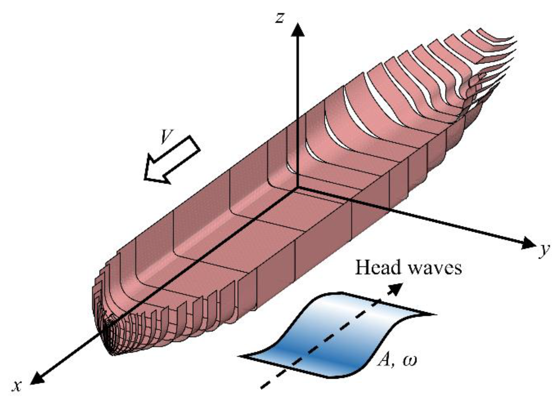
To evaluate the added resistance due to waves, the strip method was used to solve the two-dimensional (2D) boundary value problem at each section to obtain the velocity potential on the hull, as shown in Figure 2. The 2D solution was integrated based on the STF method [26] to calculate the hydrodynamic coefficients and motion responses. Then, the far-field method proposed by Maruo [12] was applied to calculate the added resistance of a ship moving forward in regular head waves, R_strip, as follows:

$$R_{strip}=\{\begin{array}{cc}\frac{\rho g{A}^2}{4\pi k}\left[-{\displaystyle {\int }_{-\infty }^{k_1}+}{\displaystyle {\int }_{k_2}^{\infty }}\right]\left\{{\left|C\left(m\right)\right|}^2+{\left|S\left(m\right)\right|}^2\right\}\frac{\nu \left(m+k\right)}{\sqrt{{\nu }^2-m^2}}dm& for \tau \ge \frac{1}{4}\\ \frac{\rho g{A}^2}{4\pi k}\left[-{\displaystyle {\int }_{-\infty }^{k_1}+}{\displaystyle {\int }_{k_2}^{k_3}+}{\displaystyle {\int }_{k_4}^{\infty }}\right]\left\{{\left|C\left(m\right)\right|}^2+{\left|S\left(m\right)\right|}^2\right\}\frac{\nu \left(m+k\right)}{\sqrt{{\nu }^2-m^2}}dm& for \tau <\frac{1}{4}\end{array}$$

(2)

where ρ is the density of water, and

$$k=\frac{2\pi }{\lambda }, {\omega }_e=\omega +Vk, \nu =\frac{{\left({\omega }_e+mV\right)}^2}{g}, \tau =\frac{V{\omega }_e}{g}$$

(3)

$$\begin{array}{c}{k}_1\\ k_2\end{array}\}=-\frac{g}{2V^2}\left(1+2\tau \pm \sqrt{1+4\tau }\right), \begin{array}{c}{k}_3\\ k_4\end{array}\}=\frac{g}{2V^2}\left(1-2\tau \mp \sqrt{1-4\tau }\right)$$

(4)

C(m) and S(m) are the symmetric and antisymmetric components of the Kochin function, respectively. They can be evaluated by directly using the determined velocity potentials and motion responses, and their formulation was induced by applying the Fourier transform method to the momentum conservation as follows [27]:

$$C\left(m\right)=C_7\left(m\right)+\frac{{\omega }_e\omega }{g}{\displaystyle \sum _{j=1,3,5}\frac{{\xi }_j}{A}{C}_j\left(m\right)}$$

(5)

$$S\left(m\right)=S_7\left(m\right)+\frac{{\omega }_e\omega }{g}{\displaystyle \sum _{j=2,4,6}\frac{{\xi }_j}{A}{S}_j\left(m\right)}$$

(6)

$$C_j\left(m\right)={\displaystyle {\iint }_{S_B}\left(\frac{\partial {\phi }_j}{\partial n}-{\phi }_j\frac{\partial }{\partial n}\right)e^{-\nu z+imx}\cos \left(y\sqrt{{\nu }^2-m^2}\right)dS\left(x,y,z\right)}, j=1,3,5,7$$

(7)

$$S_j\left(m\right)={\displaystyle {\iint }_{S_B}\left(\frac{\partial {\phi }_j}{\partial n}-{\phi }_j\frac{\partial }{\partial n}\right)e^{-\nu z+imx}\sin \left(y\sqrt{{\nu }^2-m^2}\right)dS\left(x,y,z\right)}, j=2,4,6,7$$

(8)

where φ_1–6 denotes the radiation potentials resulting from each mode of motion, φ₇ denotes the diffraction potential, and ξ_1–6 denotes the motion responses.

However, the added resistance due to short waves estimated in this way is less accurate because of difficulties in considering the nonlinearity of the diffracted head waves. Therefore, the short-wave correction formula (SNU formula) proposed by Yang et al. [16,17] was used to improve the accuracy, and the applied coordinate system is shown in Figure 3. The original asymptotic formula [8] was enhanced in three aspects in the SNU formula. First, the mean drift force on each section normal to the wall, ∆R_n, is modified depending on the finite draught of each section, T(x₀), as follows:

$$\Delta R_n=\frac{1}{2}\rho g{A}^2\times \frac{1}{2}\left[\frac{k_1}{k}-{\cos }^2\theta +\frac{k_2}{k}\sin \theta +\left\{{\cos }^2\theta +\frac{k_2}{k}\sin \theta \right\}{e}^{-2kT\left(x_0\right)}\right]$$

(9)

$$k_1=\frac{{\left({\omega }_e-V_{steady}k\cos \theta \right)}^2}{g}, k_2=\sqrt{k_1{}^2-k^2{\cos }^2\theta }$$

(10)

Second, the local steady velocity, V_steady, is modified to reflect the sectional area below the waterline as follows:

$$V_{steady}={\alpha }_A\left(x_0\right)V\cos \theta$$

(11)

$${\alpha }_A\left(x_0\right)=\{\begin{array}{cc}\min \left(1.0, \frac{2A\left(x_0\right)}{A_0\left(x_0\right)+A\left(x_0\right)}\right)& x_0\ge 0 \left(\mathrm{Front} \mathrm{part}\right)\\ 1.0& x_0<0 \left(\mathrm{Rear} \mathrm{part}\right)\end{array}$$

(12)

$$A\left(x_0\right)={\displaystyle {\int }_{-T\left(x_0\right)}^{0}ydz}, A_0\left(x_0\right)=y_0\times T\left(x_0\right)$$

(13)

Third, the ratio of bluntness coefficients at a draft and half of the maximum steady wave elevation, ζ₀, is calculated as follows to reflect the shape above the draft level:

$${\alpha }_B=\frac{B_f\left(z={\zeta }_0/2\right)}{B_f\left(z=0\right)}$$

(14)

$$B_f=\frac{1}{B}{\displaystyle {\int }_{\mathrm{Front} \mathrm{part}}{\sin }^2\theta n_{1}dl}$$

(15)

$${\zeta }_0=\frac{V^2}{g}\min \left(\frac{2.2}{1+F_T}\frac{\tan \overline{{\alpha }_E}}{\cos \overline{{\alpha }_E}}, 0.5\right)$$

(16)

$$F_T=\frac{V}{\sqrt{gT}}, L_C=\frac{2T{F}_T{}^2}{1+F_T},\tan \overline{{\alpha }_E}=\frac{3}{L_C{}^3}{\displaystyle {\int }_{F.P.-L_C}^{F.P.}{x}_0{y}_{0}d{x}_0}$$

(17)

Therefore, the enhanced asymptotic formula for the added resistance in short waves, R_asymptotic, can be evaluated as follows:

$$R_{asymptotic}={\alpha }_B{\displaystyle {\int }_{WL}\Delta R_n{n}_{1}dl}$$

(18)

This asymptotic formula is only valid in the short-wave region due to its main assumptions, and it corresponds to the diffraction component because the motion of the ship motion is neglected. Accordingly, the diffraction component obtained by the strip method, R_{strip,diffraction}, was extracted as expressed in Equation (19), and it was combined with the asymptotic formula as expressed in Equations (20) and (21).

$$R_{strip,diffraction}=\{\begin{array}{cc}\frac{\rho g{A}^2}{4\pi k}\left[-{\displaystyle {\int }_{-\infty }^{k_1}+}{\displaystyle {\int }_{k_2}^{\infty }}\right]\left\{{\left|C_7\left(m\right)\right|}^2+{\left|S_7\left(m\right)\right|}^2\right\}\frac{\nu \left(m+k\right)}{\sqrt{{\nu }^2-m^2}}dm,& \tau \ge \frac{1}{4}\\ \frac{\rho g{A}^2}{4\pi k}\left[-{\displaystyle {\int }_{-\infty }^{k_1}+}{\displaystyle {\int }_{k_2}^{k_3}+}{\displaystyle {\int }_{k_4}^{\infty }}\right]\left\{{\left|C_7\left(m\right)\right|}^2+{\left|S_7\left(m\right)\right|}^2\right\}\frac{\nu \left(m+k\right)}{\sqrt{{\nu }^2-m^2}}dm,& \tau <\frac{1}{4}\end{array}$$

(19)

$$R_{strip,combined}=\left(R_{strip}-R_{strip,diffraction}\right)+\left[R\left(\frac{\lambda }{L}\right)R_{asymptotic}+\left(1-R\left(\frac{\lambda }{L}\right)\right)R_{strip,diffraction}\right]$$

(20)

$$R\left(\frac{\lambda }{L}\right)=\frac{1}{2}\left[1+\tanh \left(C_1\left(C_2-\frac{\lambda }{L}\right)\right)\right]$$

(21)

Double-counting of the diffraction components is prevented by using the tangent hyperbolic function expressed in Equation (21), which is close to the value of 1 in short waves and gradually moves toward 0 in the long-wave region. Here, C₁ and C₂ were set to 5.0 and 1.2, respectively. Finally, the added resistance due to irregular waves, R_wave, can be evaluated using a linear superposition of the added resistance due to regular waves as follows:

$$R_{wave}=2{\displaystyle {\int }_0^{\infty }\frac{R_{strip,combined}\left(\omega \right)}{A^2}}S\left(\omega \right)d\omega$$

(22)

where S(ω) is the wave spectrum for the condition of head waves.

2.3. Estimation of Speed Loss

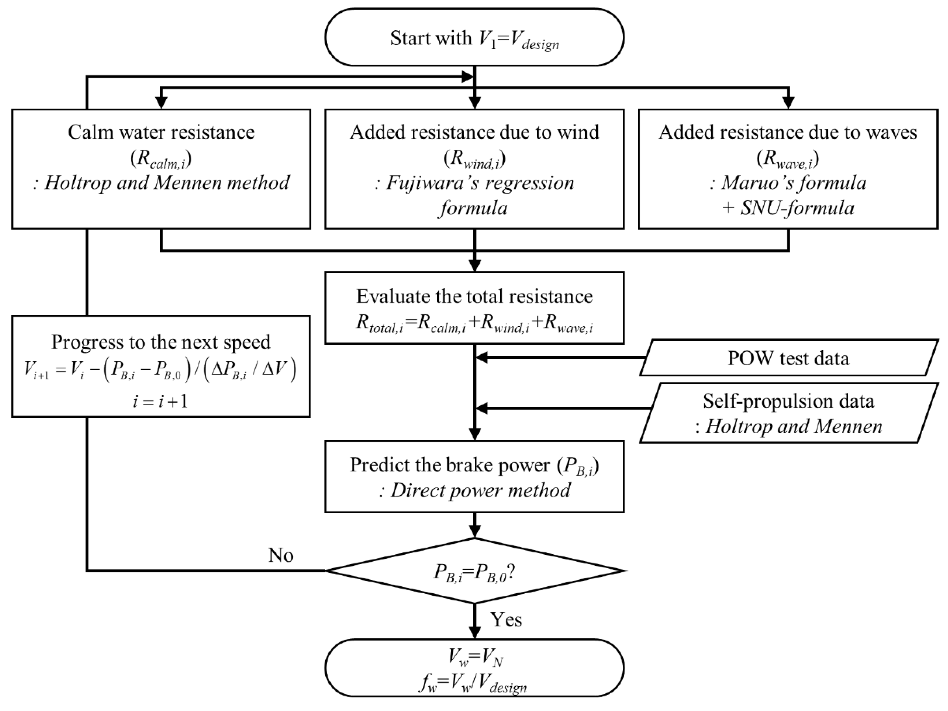
The weather factor, f_w, is included in the formulation of EEDI established by the IMO and is the value of V_w/V_design corresponding to the speed loss in representative sea conditions. Here, V_w is the value of the speed of the ship where the brake power in representative sea conditions equals the brake power required to achieve the design speed V_design in calm sea conditions [23]. Therefore, the value of 1-f_w was selected as the second objective function in this study. Using the determined total resistance, results from a propeller open water (POW) test, and self-propulsion data, the required brake power can be estimated by using the direct power method from ISO 1501 [28], as shown in Figure 4. First, the K_T/J² curve can be obtained from the POW results and using Equation (23) the advance ratio J can be calculated.

$$\frac{K_T}{J^2}=\frac{1}{\rho V_i{}^2{D}_P{}^2}\frac{R_{total}}{\left(1-t\right){\left(1-w\right)}^2}$$

(23)

where D_P is the diameter of the propeller, t is the thrust deduction coefficient, and w is the wake fraction. Here, factors on self-propulsion data were calculated using the Holtrop and Mennen method [24], assuming that these values in calm sea conditions can also be used in representative sea conditions. Next, using the obtained advance ratio, the revolution of the propeller, n, can be obtained as described in Equation (24), and the brake power can be calculated as described in Equation (25):

$$n=\frac{\left(1-w\right)V_i}{J{D}_P}$$

(24)

$$P_{B,i}=\frac{2\pi \rho D_P{}^5{n}^3{K}_Q}{{\eta }_S{\eta }_R}$$

(25)

where η_S is the transmission efficiency, which is the ratio of delivered horsepower to brake horsepower, and η_R is the relative rotative efficiency of the propeller. Then, it is repeated by changing the speed using the Newton–Raphson method until the ith obtained brake power, P_B,i, is equal to the brake power for the design speed in calm sea, P_B,0, and the ratio of the converged speed to the design speed corresponds to the weather factor.

2.4. Deformation of Hull Form

To derive the optimal hull form, four geometric parameters were selected related to operational efficiency. They were set to design variables in the GA process so that each individual had a different hull shape. The first design variable is the prismatic coefficient, C_P, which represents the bluntness of the hull. The deformation of this parameter corresponds to a global variant rather than the local variant of the hull, which is mainly used in the conceptual design phase. In the study by Jung and Kim [20], significant differences in operational efficiency for a KVLCC2 tanker due to changes in this parameter were observed. The second design variable is the waterline length, L_WL. It was expected that the bow entrance angle, the shape of the waterline, and the length of the bulbous bow would be affected by this parameter. The third design variable is the waterplane area coefficient, C_WP. It was intended to have a focused deformation of the waterline at the draft level through this parameter. Bolbot and Papanikolaou [18] showed that the C_WP had the greatest correlation to the added resistance due to waves than the other design variables, such as the waterline shape, waterline entrance angle, and flare angle. The fourth design variable is the flare angle coefficient, C_flare, in which the greater the positive value, the more the flare tilts outward. Because this deformation mainly deforms the hull form above the draft level, it was expected that it would have a significant effect on the ratio of the bluntness coefficient (see Equations (14)–(16)) of the applied SNU formula. Furthermore, the deformations of L_WL, C_WP, and C_flare were applied only to the front part of the hull because the diffraction component of the added resistance is greatly affected by the bow shape.

In this study, the hull form was implemented in the form of a non-uniform rational B-spline (NURBS) surface. Then, the cross-sectional curve can be obtained by performing an intersection between this NURBS surface and the plane at a particular station. This cross-sectional curve is defined as the NURBS curve with parameter t, and the offset points on the curve can also be extracted by varying t from 0 to 1. Figure 5 shows the NURBS surface, NURBS curves, and offset points for an example hull form. The deformation of the cross-sectional curves rather than the NURBS surface was applied in the present study, which reduced the required time for the optimization algorithm. Additionally, the automation of the deformation was relatively simple to apply and direct coupling between the deformation module and the strip method was possible because the hull form input of the strip method was also the cross-sectional curves.

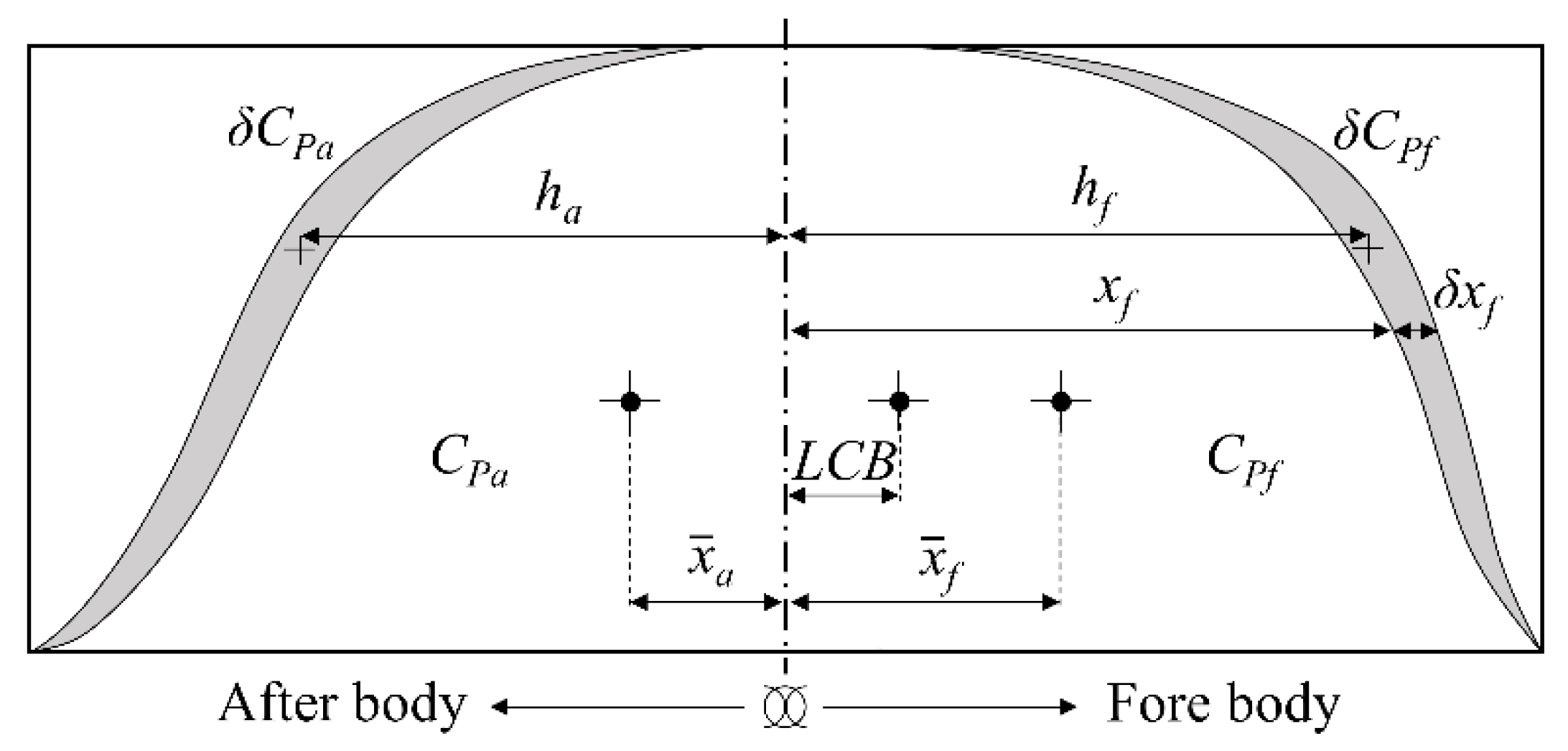
The deformation methods for each design variable of the hull form are as follows. For the variation of C_P, the 1-C_P variation method was applied. This is a method of adjusting the displacement by simply moving the cross sections in the longitudinal direction while maintaining the geometry of cross-sections of the original hull form [29], as shown in Figure 6. The longitudinal shifting distance of any section using the C_P curve of a given ship can be calculated using Equation (26). Here, δC_Pf and δC_Pa are the change in C_P values at the forepart and afterpart, respectively (Equation (27)). In addition, LCB is the distance from the midship to the longitudinal center of buoyancy, and this value was set to a fixed value. h_f and h_a are the distances from the midship to the center of δC_Pf and δC_Pa, respectively (Equation (28)). Thus, this method can produce a deformed hull form with the desired value of C_P variation.

$$\delta x_{f,a}=\frac{\delta C_{Pf,Pa}}{1-C_{Pf,Pa}}\left(1-x_{f,a}\right)$$

(26)

$$\delta C_{Pf}=\frac{2\left\{\delta C_P\left(h_a+LCB\right)\right\}}{h_f+h_a}, \delta C_{Pa}=\frac{2\left\{\delta C_P\left(h_f-LCB\right)\right\}}{h_f+h_a}$$

(27)

$$h_{f,a}=\frac{C_{Pf,Pa}\left(1-2{\overline{x}}_{f,a}\right)}{1-C_{Pf,Pa}}$$

(28)

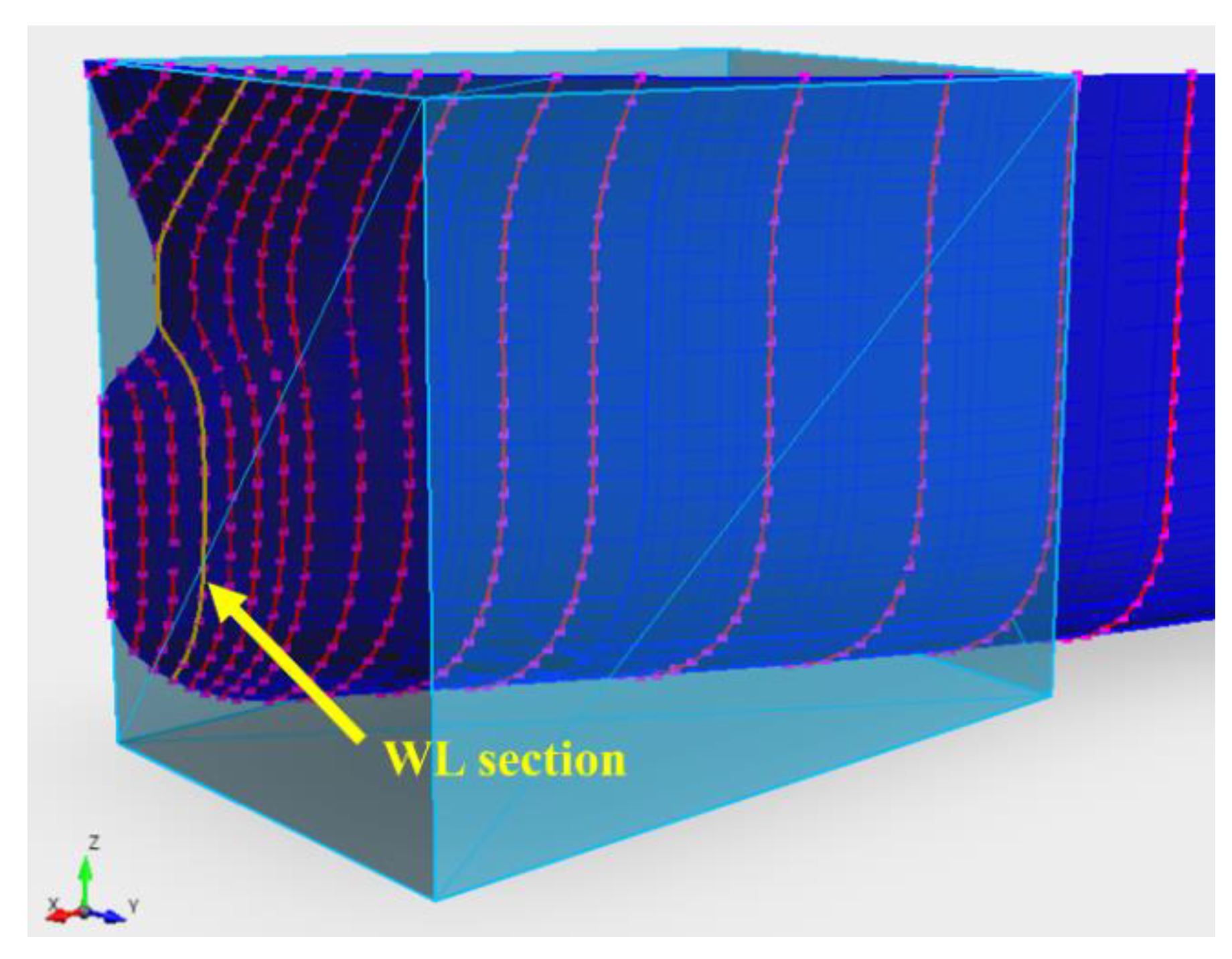
For the variation of the L_WL, first, the front section at the draft level was designated as “WL section”, as shown in Figure 7, and it was shifted in the longitudinal direction by the desired distance, ΔL_WL. The deformation range was then set from the foremost section to the forward shoulder to create a cuboid box, in which all sections in the box were shifted keeping a relative position. For example, if a section is placed in the center between the WL section and the foremost section, the middle position of this section is still maintained after the L_WL variation is performed. This allowed the forepart to maintain a smooth curvature after the deformation. As with the first design variable, the cross-sectional geometry was not changed in this method.

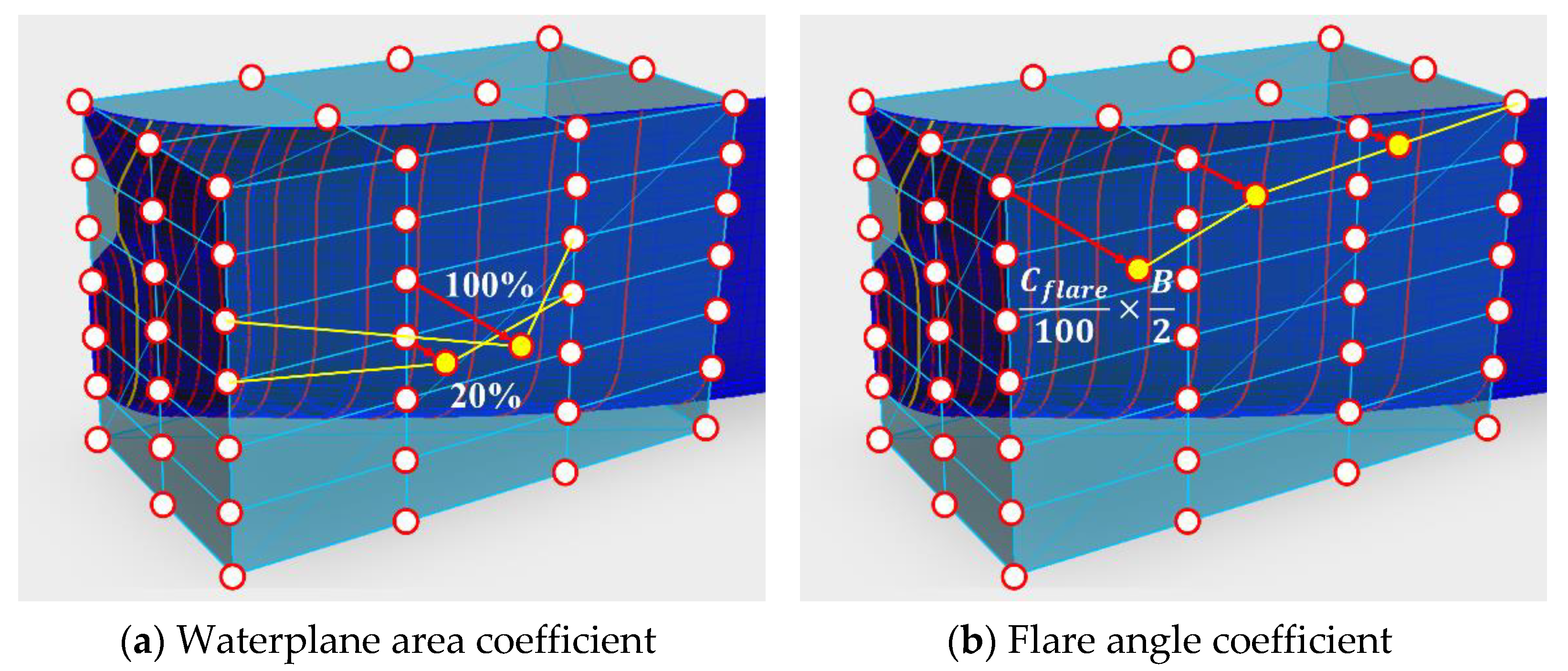
Deformations of the C_WP and C_flare were conducted using the free-form deformation (FFD) method [30]. This method constructs a grid surrounding a three-dimensional object that is to be deformed, distributes control points at the vertices of the grid, and moves them to allow a smooth deformation of the shape. In this study, the cuboid box produced for the deformation of the L_WL was also used in the FFD method, as shown in Figure 8. Thus, for C_WP, the deformation was performed by moving control points around the draft level in the breadth direction. For C_flare, the uppermost control points were moved in the breadth direction, and the percentage value of the shifting distance of the outermost control points to the half-breadth was defined as the C_flare. The control points located in front were moved further so that the front part where the incident waves were diffracted would be more deformed.

3. Results and Discussion

3.1. Target Ship

The target ship to be optimized to reduce both total resistance and speed loss is an S-VLCC tanker designed by Samsung Heavy Industries, whose principal dimensions, and other specifications for the estimation of the weather factor, are listed in

Table 2. Specifications of S-VLCC tanker.

Particulars	Values
Length between perpendicular	323.0 m
Waterline length	329.7 m
Breadth	60.0 m
Draft	21.0 m
Block coefficient	0.8106
KG	17.316 m
LCG (from A.P.)	170.803 m
Ixx/B, Iyy/LPP, Izz/LPP	0.258, 0.239, 0.242
Rudder area	273.3 m2
Propeller diameter	10.0 m
Expanded area ratio of propeller	0.4431
Transverse projected area above waterline	920.0 m2

.

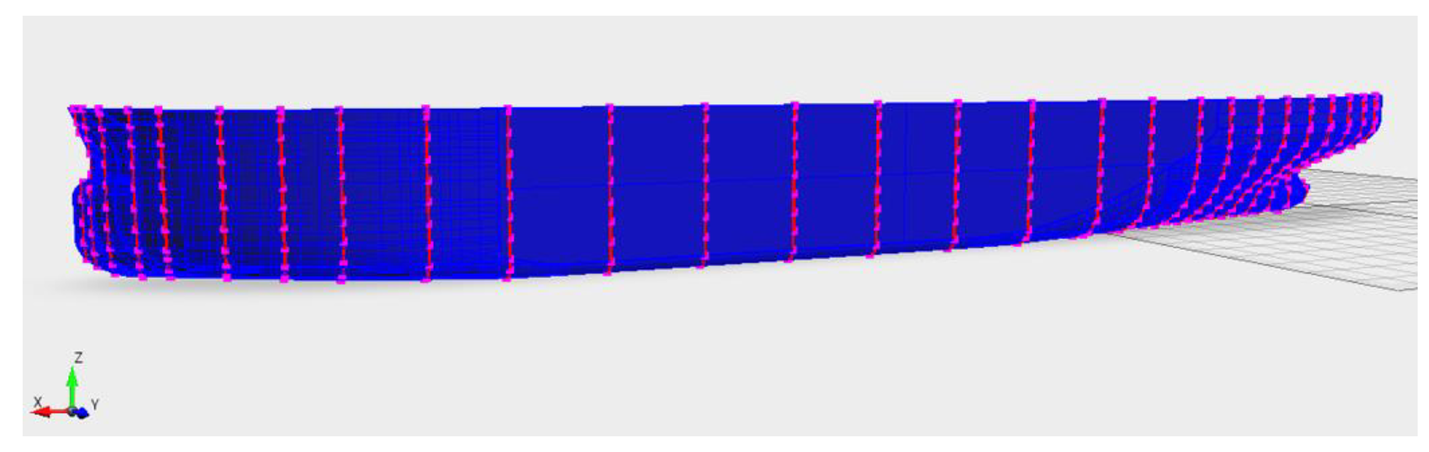
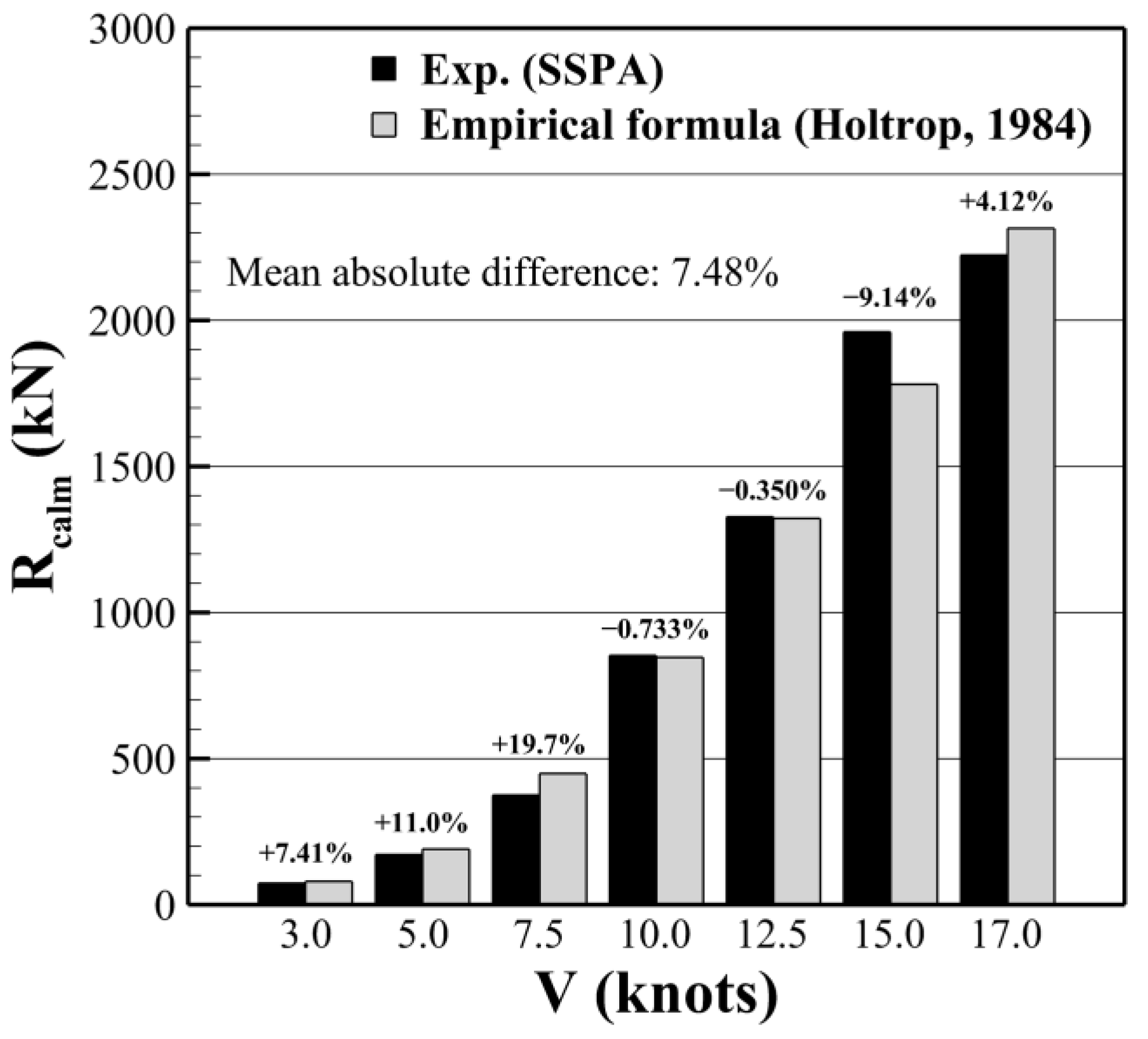
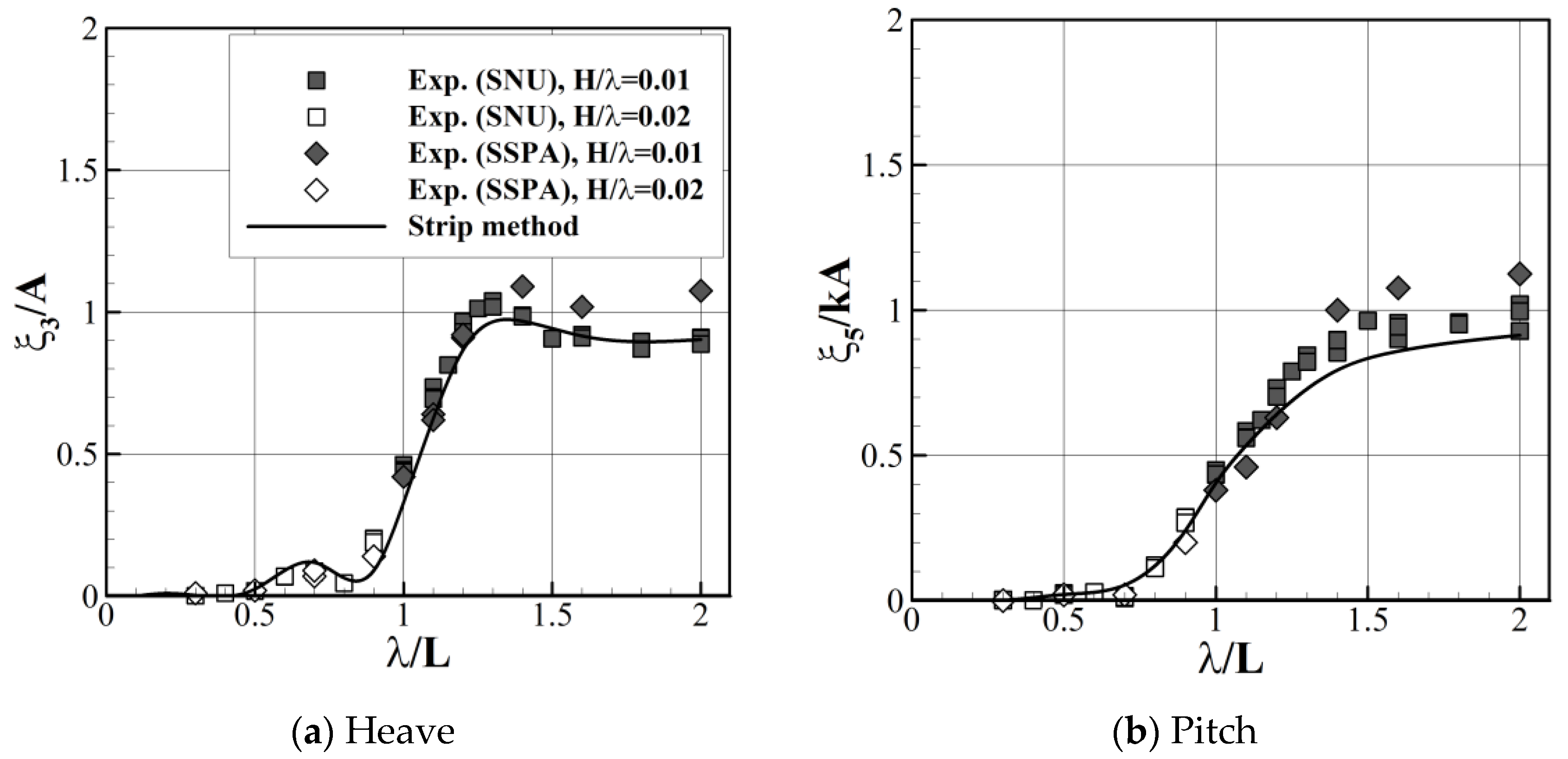
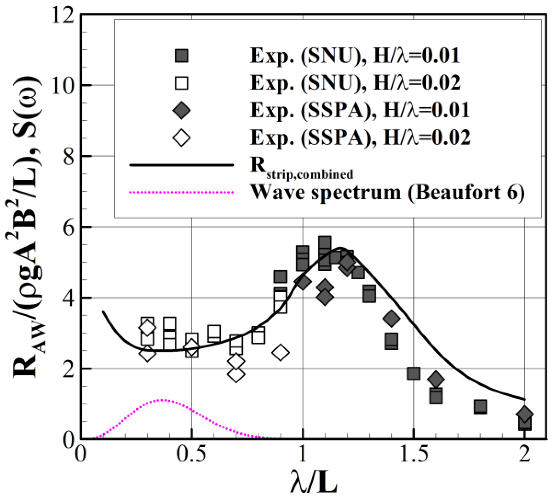
To verify the accuracy of the analysis methods applied in this study, the calculated results were compared with the results of self-propulsion experiments conducted with a 1/68 scale model in a seakeeping basin from SSPA Sweden AB [31]. The hull form model used for the numerical calculation can be found in Figure 2, with 32 sections and up to 70 offset points for each section. The front and rear parts of the hull were denser in sectional density because the shape varies greatly along the longitudinal direction. It was confirmed that the converged calculation results had been obtained with the sufficient panel density of the target model. First, the comparison of the calm water resistance results are shown in Figure 9. The experiment measured the resistance at seven ship speeds. The extensions to the full-scale values were performed by the three-dimensional extrapolation method recommended by the International Tank Towing Conference. Figure 9 shows that the empirical formula [24] applied in this study produced results consistent with the experimental values at all speeds, and the average deviation from the experiment was low at 7.48%. The motion responses in the head sea condition at the design forward speed (Fn = 0.137) are shown in Figure 10. Additionally, experimental results conducted with a 1/100 scale model in an SNU towing tank [31] are also displayed. As Figure 10 shows, the motion responses predicted by the strip method were consistent with the experimental values. Figure 11 also shows that the estimated results of the added resistance due to waves (see Equation (20)) were consistent with the experimental values. In particular, the wave spectrum of Beaufort 6 is concentrated in the short-wave region owing to the large length of the target ship. This is the wavelength region dependent on the short-wave correction formula (SNU formula). Thus, for the calculation of added resistance in representative sea conditions (R_wave), and for the evaluation of the two objective functions, it is important to accurately reflect the deformation of the hull form.

3.2. Sensitivity Analysis of Added Resistance Due to Waves

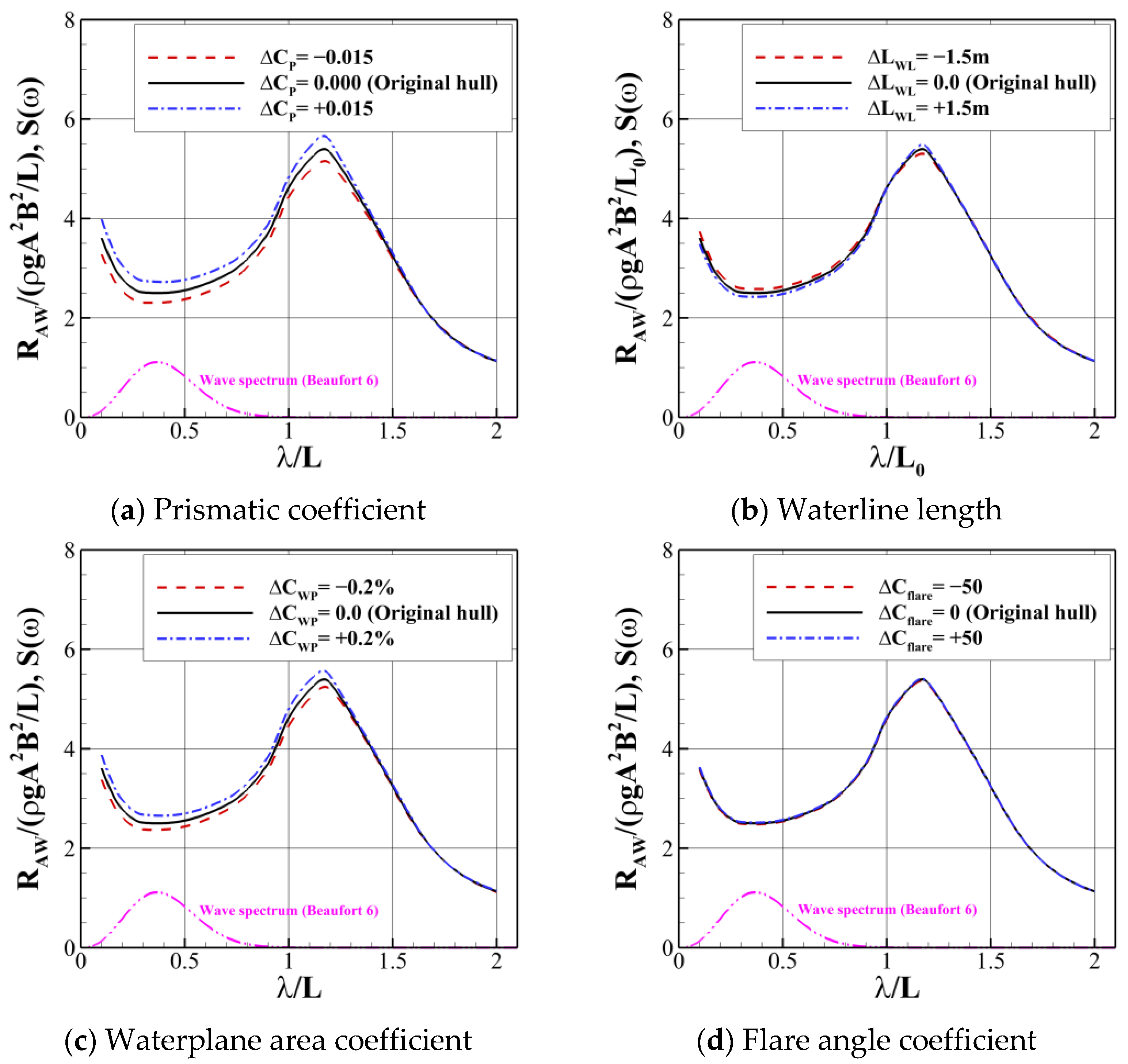
A sensitivity analysis was conducted to determine how the added resistance due to waves in the applied prediction method changed as each design variable varied. The range of the cuboid box for the deformation of the front part was designated from the foremost to the 18th station. In addition, five control points in the longitudinal direction, seven points in the depth direction, and three points in the breadth direction were distributed on the surface and inside the box for the FFD method. Figure 12 shows the difference in the transfer function of the added resistance due to waves with variations of each design variable (negative or positive) compared to the original ship. For the prismatic coefficient, the added resistance in the short-wave region where the Beaufort 6 wave spectrum was concentrated decreased as the value of C_P was reduced. To determine the reasons, several factors dependent on the SNU formula were analyzed. With respect to the deformation of C_P, the sectional area coefficient in Equation (12), α_A, did not change because the shapes of the sections remained fixed. While the entrance angle of the front part in Equation (17), α_E, might change the steady wave elevation, eventually the ratio of the bluntness coefficient in Equation (14), α_B, would be slightly changed because the hull of the target ship is nearly wall-sided at the height around the draft level. On the other hand, as the waterline profile at the draft level became thinner, θ decreased in all positions (see Figure 3), so the velocity of steady flow parallel to the wall in Equation (11), V_steady, was also changed. Above all, k₁ and k₂ in Equation (10), corresponding to the wavenumber of incident waves and outgoing diffracted waves, respectively, were also modified at each position. This indicates that when the hull shape became thinner as the value of C_P was reduced, the decrease in the momentum of the disturbed waves was the most likely factor that reduced the added resistance in short waves. Meanwhile, appropriate ranges and constraints on this variable need to be imposed to prevent excessive hull deformation, which will be discussed later.

The upper limit of the deformation of L_WL was limited to 1.5 m owing to the short length of the bulbous bow of the target ship. The results were nondimensionalized by L_BP of the original ship, L₀, to compare with the results for the original ship. As with the deformation of C_P, the variation in α_A and α_B was negligible because this deformation also maintained the sectional geometry. In addition, the bluntness of the hull decreased as L_WL increased, so the added resistance in short waves decreased for the same reason that C_P decreased. However, the length of the bulbous bow was changed, unlike the deformation of C_P, so the effect on the calm water resistance should also be carefully considered in the deformation of L_WL. Although it is outside the valid region of the wave spectrum, it is interesting that the tendency of the added resistance to change was reversed, so the added resistance increased as L_WL increased if the wavelength ratio was above 1.0. In this region, increasing L_WL improved the restoring performance, similar to the increase in C_P, which changed the motion responses to the same trend. Eventually, both increased the radiation component of added resistance. Therefore, the different tendencies of radiation components in the moderate- and long-wavelength regions for L_WL deformation need to be considered when optimizing for rougher sea conditions.

C_WP was set to change by up to 0.2% based on the value for the original ship. Unlike the deformation of C_P and L_WL, this method focused on deforming the cross-sectional shape around the draft level and the waterline profile at the front part, which affects most of the factors in the SNU formula. The added resistance in short waves also decreased as the hull shape became thinner. Because this deformation corresponds to the local deformation limited to the forward shoulder around the draft level, it implies that the added resistance can be adjusted more efficiently with little change in the hydrostatic properties of the hull by this deformation.

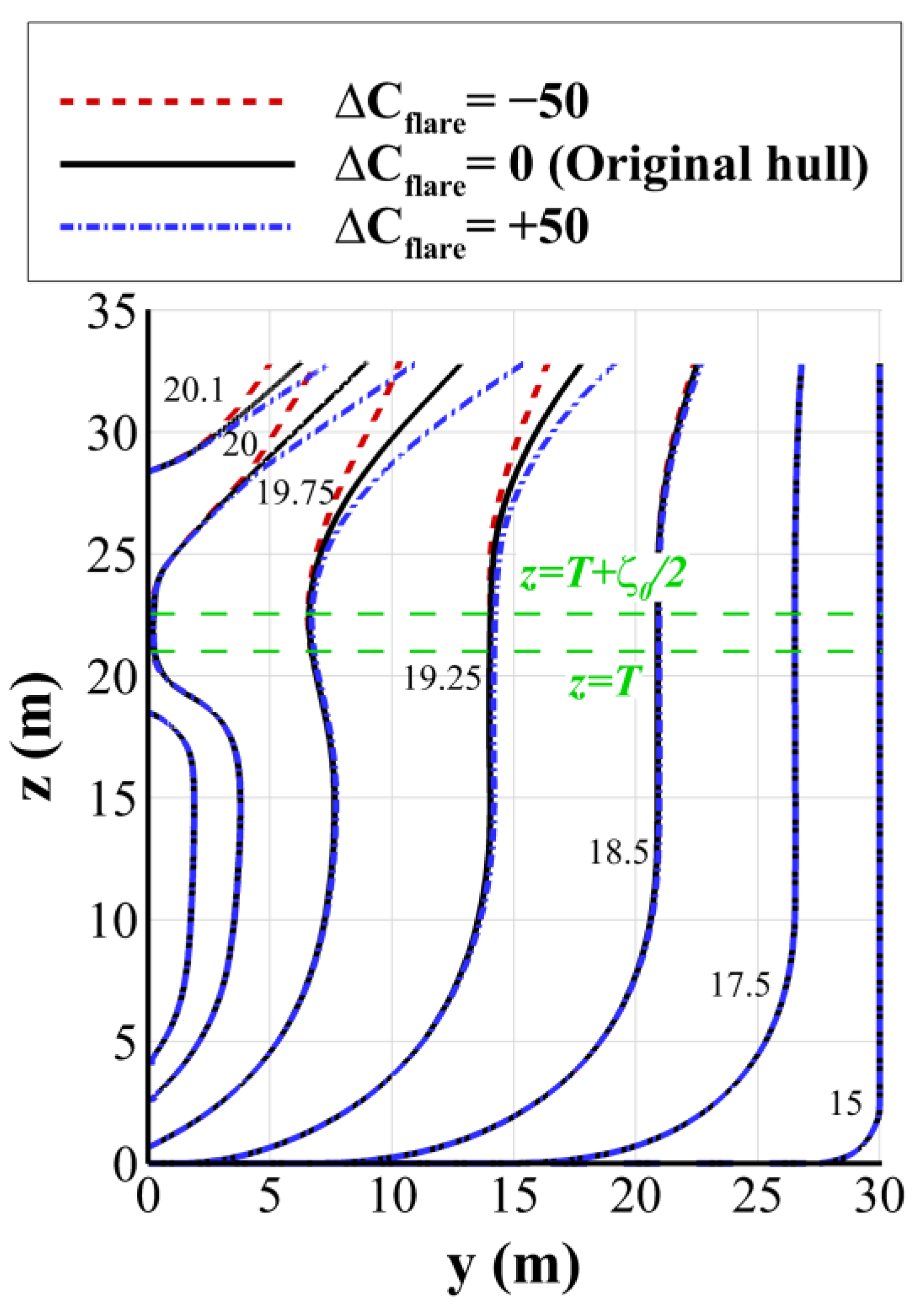
C_flare was set to 50 for both the upper and lower limit, and the deformed body plans of each limit are shown in Figure 13. In the SNU formula, the deformation above the waterline can be reflected when considering the rise in the steady wave elevation in Equation (16), ζ₀, and the ratio of the bluntness coefficient at the two heights, α_B. However, because the front part of the S-VLCC hull is close to the vertical wall at the draft level and even at the elevated level (z = T + ζ₀/2), the added resistance in short waves was very slightly reduced when C_flare was reduced. Changes in hydrodynamic performance due to the deformation of the flare angle would be apparent when the hull is more laid at the draft level, such as for container ships, or when the design speed is relatively high, so the value of the steady wave elevation is large. The overall results of the sensitivity analysis are summarized in

Table 3. Summary of the sensitivity analysis of added resistance in waves.

Design Variable	Involved Factors	Changing Direction to Decrease Added Resistance in Short Waves
Prismatic coefficient (CP)	θ, Vsteady, k1, k2	Decreasing
Waterline length (LWL)	θ, Vsteady, k1, k2	Increasing
Waterplane area coefficient (CWP)	αA, αB, θ, Vsteady, k1, k2	Decreasing
Flare angle coefficient (Cflare)	ζ0, αB	Decreasing

.

3.3. Optimization of the Hull Form

Table 4. Established problem for the hull form optimization of an S-VLCC tanker.

Elements	Items
Design variables and ranges	Prismatic coefficient: $x_1=\Delta C_P\in \left[-0.015, 0.015\right]$
	Waterline length: $x_2=\Delta L_{WL}\in \left[-1.5 \mathrm{m}, 1.5 \mathrm{m}\right]$
	Waterplane area coefficient: $x_3=\Delta C_{WP}\in \left[-0.2\%, 0.2\%\right]$
	Flare angle coefficient: $x_4=\Delta C_{flare}\in \left[-50, 50\right]$
Objective functions	Total resistance: $F_1\left(x\right)=R_{total}\left(x\right)$
	Speed loss: $F_2\left(x\right)=1-f_w\left(x\right)$
Constraints	LCB from A.P. (m): $\pm 1\%$
	Displacement (m3): $\pm 0.5\%$
	LOA (m): fixed

summarizes the established problem to perform hull form optimization of an S-VLCC tanker considering operational efficiency. The design variables were the four geometric parameters defined earlier, and the same variation ranges of each design variable in the sensitivity analysis were applied to the optimization. The two objective functions to be reduced simultaneously were the aforementioned total resistance and speed loss. Finally, to prevent excessive deformation of the hull, the constraints were established so that the distance from A.P. to LCB would vary within 1%, the displacement would vary within 0.5%, and the overall length would be fixed. It is important to note that because the design variables must be dependent on each other, each range value specifies only an independent range of deformation and does not limit the actual value of the corresponding variable during the optimization process as the constraints do.

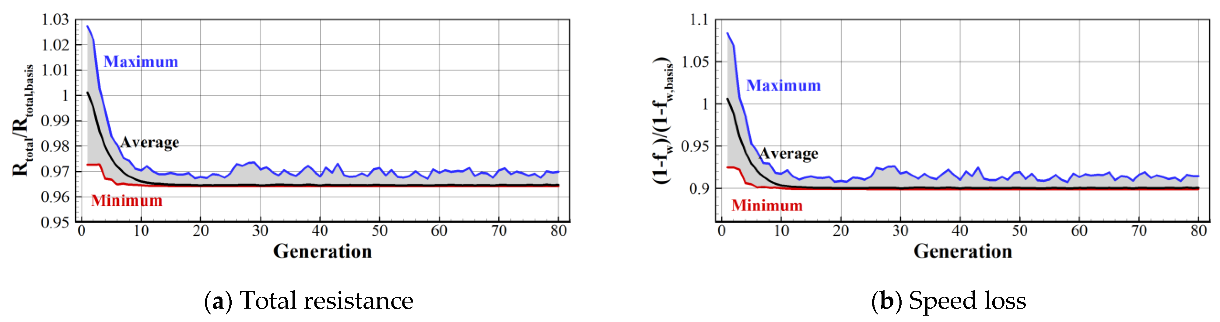
The calculation for the genetic algorithm was performed for up to 80 generations with populations of 100. This optimization result is shown in the objective space in Figure 14. The values of two objective functions for each individual were normalized with respect to the values for the original hull, so the original hull is located at (1, 1). In the first generation, it was confirmed that the individuals were evenly distributed based on the original hull. In the last generation, every individual was congregated in the lower left, which indicates that the values of both objective functions are reduced, so the individual closest to the origin was designated as the optimum solution.

The change in the normalized values of the two objective functions as the generation progressed is shown in Figure 15. In the first generation, the average value was close to 1, and as the generations progressed, the minimum and average values converged to a specific value. Because the optimization results were judged to converge from the 20th generation, the number of generations applied to the present calculation could be considered sufficient to obtain convergent optimization results.

The optimization results of the selected optimum hull are summarized in

Table 5. Optimization results of S-VLCC tanker.

Items		Original Hull	Optimum Hull	Difference
Design variables	x1 = ΔCP	0	−0.015	−0.015
	x2 = ΔLWL (m)	0	+1.5	+1.5
	x3 = ΔCWP (%)	0	−0.2	−0.2
	x4 = ΔCflare	0	−50	−50
Constraints	LCB (m)	170.97	170.01	−0.562%
	Displacement (m3)	328,583	327,707	−0.267%
	LOA (m)	332.7	332.7	-
Objective functions	F1 = Rtotal (kN)	2325.0	2241.8	−3.58%
	F2 = 1 − fw	0.1232	0.1107	−10.2%
Associated values	Rcalm (kN)	1793.2	1772.6	−1.15%
	Rwave (kN)	358.97	296.37	−17.4%
	PB (MW)	29.330	27.979	−4.61%

by comparing it with the original hull. First, it was determined that the hull form was optimum when the values of C_P, C_WP, and C_flare are the values of the lower bound and L_WL is the value of the upper bound. This is the same as the conclusion of the sensitivity analysis performed independently for each design variable (see Table 3). This indicated that even if the four design variables were simultaneously varied, it could be inferred that the trend of deformation had not changed due to the interference of the design variables. The modified hull forms corresponding to these design variables are compared to the original hull in Figure 16. As can be seen, the front of the hull became thinner and the length of the bulbous bow became much shorter (from 3.2 to 1.7 m) because of the lengthened waterline with the fixed condition of the overall length. The obtained optimum hull form can be considered similar to the LEADGE-bow shape, which has a vertical sharp edge starting from the front of the bulbous bow. In a previous study [32], towing tank experiments were conducted by comparing the added resistance due to waves of the original shape and LEADGE-bow shape of a KVLCC2 tanker. There was a significant decrease in the added resistance in short waves lying outside the uncertainty boundary. The lowered reflected bow waves were visually confirmed for the LEADGE-bow shape. This was regarded as the reason for the reduction in the diffraction component of the added resistance and it is consistent with the previous explanation about the cause of the decrease in added resistance in short waves, as the hull became thinner in the sensitivity analysis of this study. In addition, this tendency of deformation is similar to the hull form that optimizes the total resistance of the KVLCC2 tanker [18] and the hull form that optimized both the calm water resistance and the added resistance in short waves of a Supramax class bulk carrier [19]. The estimated added resistance due to waves of the original hull and the optimum hull is shown in Figure 17, and it was confirmed that a significant reduction was achieved in the short-wavelength region. It was also confirmed that all the constraint conditions were satisfied, which indicates that the obtained hull form that both optimizes the total resistance and the speed loss can be regarded as a valid form.

For the objective functions, the total resistance was reduced by 3.58% and the speed loss was reduced by 10.2%. A further comparison of the total resistance by component resulted in a significant reduction of 17.4% in the added resistance in the Beaufort 6 wave spectrum, although the calm water resistance was slightly reduced. This indicates that hull form optimization that had previously been performed, which only reduced the calm water resistance, might result in a different conclusion from the hull form optimization of ships operating in real seaways. Moreover, when it is necessary to improve the speed loss of ships in line with the EEDI regulation, the obtained results suggest that the added resistance due to waves should be reduced. However, it should be noted that the applied empirical method for the estimation of the calm water resistance and the strip method for estimating the added resistance may be somewhat incomplete to thoroughly reflect the hull form deformation. To apply a more sophisticated numerical method, it was difficult to implement automation that discretized every hull model for the valid input, and above all, it may take much more time to evaluate every objective function for a large number of individuals. Therefore, future work should be conducted by applying a numerical method that can improve accuracy while taking a computation time similar to the methods applied in this study. Finally, it was estimated that the brake power required for ships operating in the representative sea condition had decreased by approximately 4.61%.

4. Conclusions

In this study, hull form optimization that simultaneously reduced the total resistance and speed loss of an S-VLCC tanker operating under the representative sea condition defined by the IMO was conducted. To this end, design variables related to operational efficiency were selected and a sensitivity analysis was conducted to investigate the changes in added resistance in short waves due to the variation of these design variables. Furthermore, the NSGA-II algorithm was applied to perform multi-objective optimization, and it was confirmed that the derived optimum hull form showed significant improvements in results relative to the original hull. Thus, the following conclusions can be drawn:

• The prismatic coefficient (C_P), waterline length (L_WL), waterplane area coefficient (C_WP), and flare angle coefficient (C_flare), which are the shape factors associated with the operational efficiency of ships in waves, were derived. Practical methods to determine the deformation of the hull form for each design variable were presented;
• It was confirmed that results from the applied numerical methods were very consistent with the experimental results, while the computational speed was fast enough to be used for the optimization algorithm. Furthermore, the sensitivity analysis of the added resistance due to short waves estimated by these methods found that when C_P, C_WP, and C_flare decreased while L_WL increased, the added resistance in short waves decreased;
• The optimum hull form obtained within the range of variation and constraints became thinner and longer, and the length of the bulbous bow became shorter, which is similar to the LEADGE-bow shape. This is a similar conclusion to previous studies on the reduction in added resistance due to waves. In addition, an analysis of the effects of the SNU formula’s variables suggested that the distribution of k₁ and k₂, corresponding to the wavenumber of incident waves and outgoing diffracted waves, respectively, at each position, was changed, resulting in a decrease in the momentum of the diffracted waves;
• The applied optimization algorithm satisfied some elements of the genetic algorithm, such as random distributions of individuals within the range, improvements of solutions over generations, and convergence of the solution within the chosen number of generations. Both the total resistance and speed loss were significantly reduced, and in particular, it was confirmed that the tendency of the hull form optimization in terms of operating efficiency could be changed by the fact that the added resistance due to waves was significantly reduced compared to the calm water resistance.

References

- Papanikolaou, A. Holistic ship design optimization. Comput. Aided. Des. 2010, 42, 1028–1044. [Google Scholar] [CrossRef]
- Weinblum, G.P. Applications of wave resistance theory to problems of ship design. Trans. Inst. Eng. Shipbuild. Scotl. 1959, 102, 119–163. [Google Scholar]
- Dawson, C.W. A practical computer method for solving ship-wave problems. In Proceedings of the 2nd International Conference on Numerical Ship Hydrodynamics, Berkeley, CA, USA, 19–21 September 1977; The National Academies Press: Washington, DC, USA, 1977; pp. 30–38. [Google Scholar]
- Jensen, G.; Söding, H.; Mi, Z.X. Rankine source methods for numerical solutions of the steady wave resistance problem. In Proceedings of the 16th Symposium Naval Hydrodynamics, Berkeley, CA, USA, 13–18 July 1986; National Research Council: Washington, DC, USA, 1986; pp. 575–582. [Google Scholar]
- Larsson, L.; Kim, K.J.; Esping, B.; Holm, D. Hydrodynamic optimization using SHIPFLOW. In Proceedings of the 5th International Symposium on the Practical Design of Ships and Mobile Units, Newcastle, UK, 17–22 May 1992; Elsevier Applied Science: London, UK; New York, NY, USA, 1992. [Google Scholar]
- Papanikolaou, A.; Kaklis, P.; Koskinas, C.; Spanos, D.A. Hydrodynamic optimization of fast displacement catamarans. In Proceedings of the 21st International Symposium on Naval Hydrodynamics, Trondheim, Norway, 24–28 June 1996; The National Academies Press: Washington, DC, USA, 1996. [Google Scholar]
- International Maritime Organization (IMO). Amendments to the Annex of the Protocol of 1997 to Amend the International Convention for the Prevention of Pollution from Ships, 1973, as Modified by the Protocol of 1978 Relating Thereto; MEPC.203; IMO: London, UK, 2011. [Google Scholar]
- Faltinsen, O.M.; Minsaas, K.J.; Liapis, N.; Skjørdal, S.O. Prediction of resistance and propulsion of a ship in a seaway. In Proceedings of the 13th Symposium on Naval Hydrodynamics, Tokyo, Japan, 6–10 October 1980; Shipbuilding Research Association of Japan: Tokyo, Japan, 1980; pp. 505–529. [Google Scholar]
- Bunnik, T. Seakeeping Calculations for Ships, Taking into Account the Non-Linear Steady Waves. Ph.D. Thesis, Delft University of Technology, Delft, The Netherlands, 1999. [Google Scholar]
- Joncquez, S.A.G. Second-Order Forces and Moments Acting on Ships in Waves. Ph.D. Thesis, Technical University of Denmark, Copenhagen, Denmark, 2009. [Google Scholar]
- Kim, K.H.; Kim, Y. Numerical study on added resistance of ships by using a time-domain Rankine panel method. Ocean Eng. 2011, 38, 1357–1367. [Google Scholar] [CrossRef]
- Maruo, H. Wave resistance of a ship in regular head seas. Bull Fac. Eng. Yokohama Natl. Univ. 1960, 9, 73–91. [Google Scholar]
- Salvesen, N. Added resistance of ships in waves. J. Hydronaut. 1978, 12, 24–34. [Google Scholar] [CrossRef]
- Kashiwagi, M. Added resistance, wave-induced steady sway force and yaw moment on an advancing ship. Ship. Technol. Res. (Schiffstechnik) 1992, 39, 3–16. [Google Scholar]
- Seo, M.G.; Yang, K.K.; Park, D.M.; Kim, Y. Comparative study on computation of ship added resistance in waves. Ocean Eng. 2013, 73, 1–15. [Google Scholar] [CrossRef]
- Yang, K.K.; Kim, Y.; Jung, Y.W. Enhancement of asymptotic formula for added resistance of ships in short waves. Ocean Eng. 2018, 148, 211–222. [Google Scholar] [CrossRef]
- Yang, K.K.; Kim, B.S.; Kim, Y. Estimation of added resistance of ships in short oblique waves. In Proceedings of the 13th Pacific-Asia Offshore Mechanics Symposium, Jeju, Korea, 14–17 October 2018; ISOPE-PACOMS: Mountain View, CA, USA, 2018; pp. 33–40. [Google Scholar]
- Bolbot, V.; Papanikolaou, A. Parametric, multi-objective optimization of ship’s bow for the added resistance in waves. Ship. Technol. Res. (Schiffstechnik) 2016, 63, 171–180. [Google Scholar] [CrossRef]
- Yu, J.W.; Lee, C.M.; Lee, I.; Choi, J.E. Bow hull-form optimization in waves of 66,000 DWT bulk carrier. Int. J. Nav. Archit. Ocean Eng. 2017, 9, 499–508. [Google Scholar] [CrossRef]
- Jung, Y.W.; Kim, Y. Hull form optimization in the conceptual design stage considering operational efficiency in waves. Proc. Inst. Mech. Eng. M. J. Eng. Marit. Environ. 2019, 233, 745–759. [Google Scholar] [CrossRef] [Green Version]
- Kim, B.S.; Oh, M.J.; Lee, J.H.; Kim, Y.; Roh, M.I. Study on hull-form optimization considering ship operational performance in waves. In Proceedings of the 30th International Ocean and Polar Engineering Conference, Shanghai, China, 14–19 June 2020; ISOPE: Mountain View, CA, USA, 2020; pp. 3890–3896. [Google Scholar]
- Deb, K.; Pratap, A.; Agarwal, S.; Meyarivan, T. A Fast and Elitist Multiobjective Genetic Algorithm: NSGA-II. IEEE Trans. Evol. Comput. 2002, 6, 182–197. [Google Scholar] [CrossRef] [Green Version]
- International Maritime Organization (IMO). Interim Guidelines for the Calculation of the Coefficient fw for Decrease in Ship Speed in a Representative Sea Condition for Trial Use; MEPC.1/Circ.796, 12 October 2012; IMO: London, UK, 2012. [Google Scholar]
- Holtrop, J. A statistical re-analysis of resistance and propulsion data. Int. Shipbuild. Prog. 1984, 31, 272–276. [Google Scholar]
- Fujiwara, T.; Ueno, M.; Ikeda, Y. Cruising performance of a large passenger ship in heavy sea. In Proceedings of the 16th International Offshore and Polar Engineering Conference, San Francisco, CA, USA, 28 May–2 June 2006; ISOPE: Mountain View, CA, USA, 2006; pp. 304–311. [Google Scholar]
- Salvesen, N.; Tuck, E.O.; Faltinsen, O.M. Ship motions and sea loads. Trans. Soc. Nav. Archit. Mar. Eng. 1970, 78, 250–279. [Google Scholar]
- Kashiwagi, M. Calculation formulas for the wave-induced steady horizontal force and yaw moment on a ship with forward speed. Res. Inst. Appl. Mechs. Kyushu. Univ. Rpts. 1991, 37, 1–18. [Google Scholar]
- International Organization for Standardization (ISO). Ships and Marine Technology—Guidelines for the Assessment of Speed and Power Performance by Analysis of Speed Trial Data; ISO 15016; ISO: Geneva, Switzerland, 2015. [Google Scholar]
- Lackenby, H. On the systematic geometrical variation of ship forms. Trans. Royal. Inst. Naval. Arch. 1950, 92, 289–316. [Google Scholar]
- Sederberg, T.W.; Parry, S.R. Free-form deformation of solid geometric models. In Proceedings of the 13th Annual Conference on Computer Graphics and Interactive Techniques, Dallas, TX, USA, 18–22 August 1986; Association for Computing Machinery: New York, NK, USA, 1986; pp. 151–160. [Google Scholar]
- Park, D.M.; Lee, J.H.; Jung, Y.W.; Lee, J.; Kim, Y.; Gerhardt, F. Experimental and numerical studies on added resistance of ship in oblique sea conditions. Ocean Eng. 2019, 186, 106070. [Google Scholar] [CrossRef]
- Lee, J.; Park, D.M.; Kim, Y. Experimental investigation on the added resistance of modified KVLCC2 hull forms with different bow shapes. Proc. Inst. Mech. Eng. M. J. Eng. Marit. Environ. 2017, 231, 395–410. [Google Scholar] [CrossRef]
Figure 1.
Flowchart of applied optimizing process (NSGA-II).
Figure 2.
Definition of the seakeeping problem applied to the strip method and panel model of an S-VLCC tanker.
Figure 3.
Coordinate system for the short-wave correction formula (SNU formula).
Figure 4.
Procedure for the estimation of the required brake power.
Figure 5.
Example of a hull form.
Figure 6.
Example of a CP curve for the 1-CP variation method.
Figure 7.
Example of the WL section and a cuboid box for the variation of waterline length.
Figure 8.
Example of the FFD method for each deformation.
Figure 9.
Comparison of calm water resistance of an S-VLCC tanker.
Figure 10.
Magnitude of heave and pitch motion of an S-VLCC tanker in head waves, Fn = 0.137.
Figure 11.
Added resistance of an S-VLCC tanker in head waves, Fn = 0.137.
Figure 12.
Sensitivity analysis of added resistance of an S-VLCC tanker in head waves, Fn = 0.137.
Figure 13.
Comparison of body plans of the front part due to the deformation of flare angle.
Figure 14.
Generational development of individuals in the objective space.
Figure 15.
Generational change of the objective functions.
Figure 16.
Comparison of the deformation of the front part of an S-VLCC hull form.
Figure 17.
Comparison of estimated results of added resistance in waves of an S-VLCC tanker.