Offset-Free Economic MPC Based on Modifier Adaptation: Investigation of Several Gradient-Estimation Techniques

Abstract

Various offset-free economic model predictive control schemes that include a disturbance model and the modifier-adaptation principle have been proposed in recent years. These schemes are able to reach plant optimality asymptotically even in the presence of plant–model mismatch. All schemes are affected by a major issue that is common to all modifier-adaptation formulations, namely, plant optimality (note that convergence per se does not require perfect plant gradients) requires perfect knowledge of static plant gradients, which is a piece of information not known in most practical applications. To address this issue, we present two gradient-estimation techniques, one based on Broyden’s update and the other one on linear regression. We apply these techniques for the estimation of either the plant gradients or the modifiers directly. The resulting economic MPC schemes are tested in a simulation and compared on two benchmark examples of different complexity with respect to both convergence speed and robustness to measurement noise.

1. Introduction

Economic model predictive control (eMPC) [1] has been proposed to overcome the traditional separation between control and optimization layers in industrial process operations [2,3]. eMPC merges standard MPC with the economic optimization layer that is characteristic of real-time optimization (RTO) [2]. In particular, this combination is obtained by substituting the MPC tracking objective with economic performance [4]. There are many similarities between MPC and eMPC, with one of the main challenges being optimality under plant–model mismatch [3]. Note that the tracking-MPC (tMPC) and RTO communities have dealt with this challenge for many years, and two main solutions have been established. The first one concerns tMPC schemes and consists of augmenting the nominal model with a disturbance model so as to generate a steady-state offset correction to set-point changes [5,6]. A comprehensive review about offset-free tMPC can be found in [7]. On the other hand, RTO formulations have incorporated the so-called modifier-adaptation (MA) idea [8,9]. The essence of the MA strategy is to force the KKT optimality conditions of the modified model to match those of the plant upon convergence by using zeroth- and first-order correction terms [10].

To handle plant–model mismatch in eMPC schemes, a methodology that combines the augmented model used in tMPC [7] and the MA approach used in RTO [8] was first proposed in [11] and labeled “offset-free eMPC” (OF-eMPC). Alternative OF-eMPC formulations have been proposed in recent years [11,12,13]. These formulations can overcome plant–model mismatch and let the controlled plant reach plant optimality upon convergence. This is done with the help of zeroth- and first-order modifier terms that exploit an alternative version of MA, labeled “output MA” (MAy). Instead of modifying the cost function and the constraints as in traditional MA [8], MAy sets the modifier terms on the outputs. A recent comprehensive analysis of MAy and its convergence properties can be found in [14].

Despite its ability to converge to plant optimality in the presence of plant–model mismatch, OF-eMPC suffers from a major caveat to proper MA schemes. Indeed, these schemes require accurate knowledge of static plant gradients with respect to inputs. This represents a major challenge, especially when dealing with noisy measurements. Even the most recent MA investigations, which strive for feasibility improvement [15], faster convergence [16], applicability to periodic systems [17], or large-scale systems [18], are still based on the assumption that the plant gradients are perfectly known. Nevertheless, several approaches for estimating plant gradients have been proposed, as detailed next.

The gradient estimation techniques found in literature can be divided into two classes [10]. The first class, and by far the largest, includes steady-state perturbation methods that rely on steady-state data (e.g., [19,20,21]). These methods are the ones that better replicate the concept of steadiness of RTO iterations. On the other hand, it might be advantageous with slow processes to use transient data and estimate steady-state gradients on the go [22,23,24]. In this case, we speak of dynamic perturbation methods, which exhibit a compromise between convergence speed and accuracy. Concretely, gradient approximations are computed using either a finite-difference approach (see [10] for an overview of available approaches) or some type of system identification [21,24,25]. Exploiting the so-called directional modifier-adaptation concept [20], recent works have shown how privileged directions can ease gradient estimation—thereby making the approach more reactive to plant–model mismatch [26,27]—and how these directions can be computed efficiently [28]. Jeong et al. [29] recently compared the performance of different gradient estimation methods with MA schemes. These methods include multivariate linear regression, partial least-squares regression, and principal component analysis. It is shown that the use of latent-variable space can result in fast convergence and stability near plant optimality.

It is worth noting that researchers have also tried to avoid working with plant gradient estimation. Navia et al. [30] formulated a nested optimization problem, in which the modifiers are computed via gradient-free optimization in the outer loop. Although the nested implementation was proved to be robust in the presence of noisy measurements and capable of reaching plant optimality, it was rather slow. Another modifier-estimation technique based on optimization has been proposed recently in [31]. In this case, the limiting factor becomes the choice of weighting factors in the optimization problem and the speed at which plant optimality can be reached.

This paper aims at investigating alternative solutions to the gradient estimation problem. In particular, we propose two main techniques to estimate static plant gradients, namely, a Broyden’s update and linear regression. Note that these techniques have already been used to estimate plant gradients and modifiers in the RTO context, but not in the control context, that is, using fast sampling time and dynamic optimization. Another important advantage over our previous work [21,25] is not requiring repeated local perturbations of the process. Moreover, taking inspiration from the aforementioned “plant gradient-free” methodologies [30,31], we also use the same two techniques to estimate the modifiers directly.

This work represents an extension to [32], but it also goes further by comparing several gradient-estimation techniques. This is important to steer future research on how MA can best be combined with eMPC.

The paper is organized as follows. The problem definition and the constituents of OF-eMPC are detailed in Section 2. Several gradient-estimation techniques based on either plant gradient estimation or modifier estimation are discussed in Section 3, while Section 4 presents two OF-eMPC algorithms. The resulting OF-eMPC schemes are then compared via a numerical example and a standard benchmark case study in Section 5. Finally, conclusions are presented in Section 6.

2. Preliminaries

The OF-eMPC algorithm described in this paper deals with a general nonlinear plant and cost. Let us detail the main concepts and techniques.

2.1. Plant and Cost Specifications

The plant to be optimized is expressed by the following discrete-time nonlinear dynamic system:

$$\begin{array}{c}{x}_p^{+}=f_p(x_p,u)\\ y_p=h_p\left(x_p\right),\end{array}$$

(1)

where $x_p\in {\mathbb{R}}^{n_{x_p}}$, $u\in {\mathbb{R}}^{n_u}$ and $y_p\in {\mathbb{R}}^{n_y}$ are the plant states, inputs, and outputs, respectively; $x_p^{+}$ are the successor states. The unknown functions $f_p:{\mathbb{R}}^{n_{x_p}}\times {\mathbb{R}}^{n_u}\to {\mathbb{R}}^{n_{x_p}}$ and $h_p:{\mathbb{R}}^{n_{x_p}}\to {\mathbb{R}}^{n_y}$ are assumed to be differentiable. The measured plant outputs $y_p$ at time $k\in \mathbb{Z}$ are noted $y_{p,k}$. Furthermore, the inputs and outputs are bounded,

$$u_{min}\le u\le u_{max},y_{min}\le y\le y_{max},$$

(2)

with $u_{min},u_{max},y_{min}$, and $y_{max}$ being the corresponding lower and higher bounds.

Plant (1) is said to be optimized when the known and differentiable function ${\ell }_e:{\mathbb{R}}^{n_y}\times {\mathbb{R}}^{n_u}\to \mathbb{R}$ is minimized. Hence, the triple $({\overline{x}}_p^{*},{\overline{u}}^{*},{\overline{y}}_p^{*})$ that defines the economic optimum equilibrium of Plant (1) can be computed as:

$$\begin{array}{c}({\overline{x}}_p^{*},{\overline{u}}^{*},{\overline{y}}_p^{*})=arg\underset{x,u,y}{min}{\ell }_e(y,u)\end{array}$$

(3)

subject to

$$\begin{array}{c}x=f_p(x,u)\end{array}$$

(4)

$$\begin{array}{c}y=h_p\left(x\right)\end{array}$$

(5)

$$\begin{array}{c}{u}_{min}\le u\le u_{max}\end{array}$$

(6)

$$\begin{array}{c}{y}_{min}\le y\le y_{max}.\end{array}$$

(7)

We introduce the following assumption about Problem (3)–(7):

Assumption 1

(Plant optimality).

• Problem (3)–(7) is feasible;
• The triple $({\overline{x}}_p^{*},{\overline{u}}^{*},{\overline{y}}_p^{*})$ is the unique solution to Problem (3)–(7).

Remark 1

(Unknown plant optimum). Given that the functions $f_p$ and $h_p$ in Equation (1) are typically unknown, the solution triple of Problem (3)–(7) is also unknown.

2.2. Nominal and Augmented Models

We consider the following nominal process model:

$$\begin{array}{c}{x}^{+}=f(x,u)\\ y=h\left(x\right),\end{array}$$

(8)

in which x and $x^{+}\in {\mathbb{R}}^{n_x}$ denote the current and successor states, respectively. It is assumed that the functions $f:{\mathbb{R}}^{n_x}\times {\mathbb{R}}^{n_u}\to {\mathbb{R}}^{n_x}$ and $h:{\mathbb{R}}^{n_x}\to {\mathbb{R}}^{n_y}$ are known and differentiable.

Remark 2

(Plant–model mismatch). The functions f and h in Equation (8) differ from the plant functions $f_p$ and $h_p$ in Equation (1) due to plant–model mismatch.

Augmenting Model (8) linearly with the integral states $d\in {\mathbb{R}}^{n_d}$, called disturbances, has proven to be very effective for improving the performance of tMPC under plant–model mismatch [5,6,33,34,35]. In the general formulation, the effects of the disturbances on the states and outputs are modeled using the matrices $B_d\in {\mathbb{R}}^{n_x\times n_d}$ and $C_d\in {\mathbb{R}}^{n_y\times n_d}$:

$$\begin{array}{cc}{x}^{+}\hfill & =F(x,u,d)=f(x,u)+B_{d}d\hfill \\ d^{+}\hfill & =d\hfill \\ y\hfill & =H(x,d)=h\left(x\right)+C_{d}d.\hfill \end{array}$$

(9)

The resulting augmented functions $F:{\mathbb{R}}^{n_x}\times {\mathbb{R}}^{n_u}\times {\mathbb{R}}^{n_d}\to {\mathbb{R}}^{n_x}$ and $H:{\mathbb{R}}^{n_x}\times {\mathbb{R}}^{n_d}\to {\mathbb{R}}^{n_y}$ are assumed to be continuous and consistent with f and h, that is, $F(x,u,0)\to f(x,u)$, $H(x,0)\to h\left(x\right)$. To guarantee that the augmented model can represent the plant without steady-state offset, we introduce the following assumption (see [35] (Remark 8)):

Assumption 2

(Observability). The augmented system (9) is observable.

2.3. State and Disturbance Estimation

At each time step, the estimation procedure includes two steps, namely, prediction and filtering. First, using the augmented model (9), one computes the predicted values ${\widehat{x}}_k,{\widehat{d}}_k$, and ${\widehat{y}}_k$ as

$$\begin{array}{c}\hfill {\widehat{x}}_k=F({\widehat{x}}_{k-1}^{*},u_{k-1},{\widehat{d}}_{k-1}^{*})\\ {\widehat{d}}_k={\widehat{d}}_{k-1}^{*}\hfill \\ {\widehat{y}}_k=H({\widehat{x}}_k,{\widehat{d}}_k),\hfill \end{array}$$

(10)

where ${\widehat{x}}_{k-1}^{*}$ and ${\widehat{d}}_{k-1}^{*}$ are the estimates of $x_{k-1}$ and $d_{k-1}$ at time $k-1$. Then, using output measurements, these predicted values are filtered appropriately to give the estimates ${\widehat{x}}_k^{*},{\widehat{d}}_k^{*}$, and ${\widehat{y}}_k^{*}$.

There are different types of estimators. For example, the so-called moving-horizon estimator (MHE) processes past output measurements in an optimization framework [36]. In contrast, a Luenberger observer or Kalman filter uses only the current measurements $y_{p,k}$ to estimate the augmented states from their predicted values. This is the type of estimator used in this study and is detailed next.

The prediction errors at time k are expressed as

$${ϵ}_k=y_{p,k}-{\widehat{y}}_k$$

(11)

and used to estimate the augmented states as follows:

$$\begin{array}{c}\hfill {\widehat{x}}_k^{*}={\widehat{x}}_k+K_x{ϵ}_k\\ \hfill {\widehat{d}}_k^{*}={\widehat{d}}_k+K_d{ϵ}_k.\end{array}$$

(12)

Note that the matrices $K_x\in {\mathbb{R}}^{n_x\times n_y}$ and $K_d\in {\mathbb{R}}^{n_d\times n_y}$ must be chosen to form an asymptotically stable observer, which implies $n_y=n_d$ and $K_d$ to be invertible [5,35].

2.4. Output Modifiers

The output-correction scheme adopted in this study follows the MAy formulation that was originally developed in the RTO literature [14] and firstly applied in the eMPC framework by [11]. The correction is based on zeroth- and first-order terms that represent the steady-state deviations between plant and model outputs. In our implementation, we use the disturbance estimates ${\widehat{d}}^{*}$ as zeroth-order corrections. The first-order modifier matrix at time k is noted ${\Lambda }_k\in {\mathbb{R}}^{n_y\times n_u}$, with ${\Lambda }_0=0$. Its evolution over time is described by the following filtering equation:

$${\Lambda }_k=(1-\sigma ){\Lambda }_{k-1}+\sigma \left({\mathrm{D}}_u{g}_p\left({\overline{u}}_{k-1}\right)-{\mathrm{D}}_{u}g\left({\overline{u}}_{k-1}\right)\right),$$

(13)

where $\sigma$ is a scalar filter constant $\in (0,1]$, the operators ${\mathrm{D}}_u(·)$ are the derivatives of the considered output functions (either $g_p$ or g) with respect to the inputs u, and ${\overline{u}}_{k-1}$ are the input steady-state targets computed at the previous iteration by the target calculation described in the next subsection.

The plant steady-state input-to-output maps $g_p:{\mathbb{R}}^{n_u}\to {\mathbb{R}}^{n_y}$ are unknown, and ${\mathrm{D}}_u{g}_p\left({\overline{u}}_{k-1}\right)$ must be estimated experimentally from input and output measurements. The model steady-state input-to-output maps $g:{\mathbb{R}}^{n_u}\to {\mathbb{R}}^{n_y}$ are calculated from Model (8) upon imposing the target inputs ${\overline{u}}_{k-1}$ as follows:

$$\begin{array}{c}\left\{\begin{array}{c}{\overline{x}}_{k-1}=f({\overline{x}}_{k-1},{\overline{u}}_{k-1})\hfill \\ {\overline{y}}_{k-1}=h\left({\overline{x}}_{k-1}\right)\hfill \end{array}\right.\Rightarrow {\overline{y}}_{k-1}=g\left({\overline{u}}_{k-1}\right).\end{array}$$

(14)

Remark 3

(Model gradients). Since a linear disturbance model is used, the derivatives of Models (8) and (9) with respect to u are identical.

2.5. Target Calculation with Modifiers

The equilibrium triple $\left({\overline{x}}_k,{\overline{u}}_k,{\overline{y}}_k\right)$ at time k is calculated via steady-state optimization. The modifiers described in Section 2.4 correct the outputs so as to eliminate any first-order plant–model mismatch. The following steady-state target problem is solved at each iteration:

$$\begin{array}{c}\left({\overline{x}}_k,{\overline{u}}_k,{\overline{y}}_k\right)=\underset{(x,u,y)}{argmin}{\ell }_e(y,u)\end{array}$$

(15)

subject to

$$\begin{array}{c}x=F(x,u,{\widehat{d}}_k^{*})\end{array}$$

(16)

$$\begin{array}{c}y=H(x,{\widehat{d}}_k^{*})+{\Lambda }_k\left(u-{\overline{u}}_{k-1}\right)\end{array}$$

(17)

$$\begin{array}{c}{u}_{min}\le u\le u_{max}\end{array}$$

(18)

$$\begin{array}{c}{y}_{min}\le y\le y_{max}.\end{array}$$

(19)

The modifier terms ${\Lambda }_k\left(u-{\overline{u}}_{k-1}\right)$ in Equation (17) ensure KKT matching between Problems (3)–(7) and (15)–(19) [11,14].

2.6. Economic MPC with Modifiers

The finite-horizon optimal control problem (FHOCP) typical of eMPC is modified similarly to the method in Equation (17). Defining the generic state and input sequences $\mathit{x}:\{{\chi }_0,{\chi }_1,\dots ,{\chi }_N\}$ and $\mathit{u}:\{{\nu }_0,{\nu }_1,\dots ,{\nu }_{N-1}\}$, the optimal problem solved over N steps at each decision time k reads

$$\begin{array}{c}({\mathit{x}}_k^{\star },{\mathit{u}}_k^{\star })=arg\underset{\mathit{x},\mathit{u}}{min}\sum _{i=0}^{N-1}{\ell }_e({\gamma }_i,{\nu }_i)\end{array}$$

(20)

subject to

$$\begin{array}{c}{\chi }_0={\widehat{x}}_k^{*}\end{array}$$

(21)

$$\begin{array}{c}{\chi }_{i+1}=F({\chi }_i,{\nu }_i,{\widehat{d}}_k^{*})\end{array}$$

(22)

$$\begin{array}{c}{\gamma }_i=H({\chi }_i,{\widehat{d}}_k^{*})+{\Lambda }_k({\nu }_i-{\overline{u}}_{k-1})\end{array}$$

(23)

$$\begin{array}{c}{u}_{min}\le {\nu }_i\le u_{max}\end{array}$$

(24)

$$\begin{array}{c}{y}_{min}\le {\gamma }_i\le y_{max}\end{array}$$

(25)

$$\begin{array}{c}{\chi }_N={\overline{x}}_k.\end{array}$$

(26)

Assumption 3

(FHOCP).

• Problem (20)–(26) is feasible
• The ordered pair $({\mathit{x}}_k^{\star },{\mathit{u}}_k^{\star })$ is the unique solution to Problem (20)–(26)

The inputs implemented in the plant are the first ones of the optimal sequence ${\mathit{u}}_k^{\star }$, that is,

$$u_k={\mathit{u}}_k^{\star }\left[1\right].$$

(27)

We remark that, since the modifier terms in Equations (17) and (23) serve the same goal, for consistency purposes, the steady-state input targets used in Problem (20)–(26) are ${\overline{u}}_{k-1}$ and not ${\overline{u}}_k$. Moreover, for ensuring closed-loop stability of eMPC at nominal conditions, the following assumption is introduced:

Assumption 4.

Steady-state operation is assumed to be more profitable than oscillating behavior, that is, the system is dissipative with respect to the stage cost ${\ell }_e(·)$ [37].

Furthermore, to be able to deal with plant–model mismatch, we also need the following assumption:

Assumption 5.

The closed-loop control sequence generated by the FHOCP (20)–(26) converges.

Note that Assumption 5 is consistent with the convergence requirements of tracking offset-free MPC [7], modifier-adaptation schemes [9,14], and offset-free economic MPC [12].

3. Gradient or Modifier Estimation

The issue limiting the practical applicability of MA methods (and thus, also of MAy), is the need to gather appropriate information about the plant–model mismatch. In particular, it is necessary to accurately estimate the steady-state plant gradients ${\mathrm{D}}_u{g}_p(·)$ for the OF-eMPC algorithm in Section 2 to work properly. As a matter of fact, convergence to plant optimality is only ensured with perfect gradient estimation [38].

3.1. Basic Idea

This section compares two methodologies based on steady-state perturbation methods. We also compare the performance when one uses only measurements taken at the current iteration versus data collected at several (previous) iterations.

In Section 2.4, the first-order modifiers ${\Lambda }_k$ are updated at every sampling time. This works fine if the plant measurements correspond to steady-state conditions; however, when dealing with transient measurements, the system must reach some sort of “steadiness” before updating ${\Lambda }_k$. For this reason, with all the methods investigated next, the modifiers are updated every M sampling times, where $M\sim \frac{{\tau }_{st}}{\tau }$ is a tuning parameter, with ${\tau }_{st}$ being the time to reach steady state and $\tau$ being the sampling time. This way, we let the system reach quasi-stationary conditions between two successive modifier updates, thereby satisfying the necessity of operating with (near) steady-state measurements. This implies a time-scale separation between the control and gradient-estimation tasks. Since ${\Lambda }_k$ is updated recursively, it helps to start the recursion with a fair estimate of $\Lambda$. In this initialization phase, we apply $n_u$ appropriate input perturbations and collect quasi-stationary output measurements, with which we can construct an initial nonzero ${\Lambda }_0$. The next two subsections will address plant gradient estimation and modifier adaptation, respectively.

3.2. Plant Gradient Estimation

We propose two techniques for the estimation of plant output gradients.

3.2.1. Broyden’s Update for Plant Gradient Estimation

Broyden’s update offers a recursive way of updating the estimated gradients using current and past measurements [10,39,40]. The advantage of Broyden’s update is that it does not require additional perturbations; however, being a numerical method, sufficient variation between two consecutive inputs is needed for the scheme not to fail. The technique is a standard secant method in nonlinear programming for updating estimates of first-order derivatives, such as Jacobian matrices [41].

At the $k^{th}$ iteration, ${\mathrm{D}}_u{g}_{p,k}$, which are estimates of ${\mathrm{D}}_u{g}_p\left({\overline{u}}_{k-1}\right)$, are updated by defining

$$\begin{array}{cc}\hfill \Delta Y_k& y_{p,k}-y_{p,k-M}\hfill \end{array}$$

(28)

$$\begin{array}{cc}\hfill \Delta U_k& u_{k-1}-u_{k-M-1}\hfill \end{array}$$

(29)

and using Broyden’s formula as follows:

$${\mathrm{D}}_u{g}_{p,k}={\mathrm{D}}_u{g}_{p,k-M}+{\displaystyle \frac{\Delta Y_k-{\mathrm{D}}_u{g}_{p,k-M}\Delta U_k}{\Delta U_k^T\Delta U_k}}\Delta U_k^T.$$

(30)

The gradients of the model output functions $g(·)$ can be computed from their definition (14) using the implicit function theorem:

$${\mathrm{D}}_{u}g(·)={\mathrm{D}}_{x}h\left(x\right)\left[{\left(I-{\mathrm{D}}_{x}f(x,u)\right)}^{-1}{\mathrm{D}}_{u}f(x,u)\right].$$

(31)

Then, the gradient differences are calculated as follows:

$$\Delta g_k={\mathrm{D}}_u{g}_{p,k}-{\mathrm{D}}_u{g}_k.$$

(32)

When applying Equation (30), care must be taken to avoid ill-conditioning when $\Delta U_k\to 0$. Hence, the step given by Equation (30) is performed only if $\parallel \Delta U_k\parallel \ge {\rho }_u$, where ${\rho }_u$ is a chosen threshold.

3.2.2. Linear Regression for Plant Gradient Estimation

This method relies on output measurements at $n_s+1$ steady-state operating points corresponding to the inputs $u_k,u_{k-M},\cdots ,u_{k-n_{s}M}$, with $n_s\ge n_u$. Using such a data set, the plant output gradients are computed as linear interpolation if $n_u=n_s$ or linear regression if $n_s>n_u$. These gradients are often called simplex gradients [42]. A similar approach is used in [43]. In the present work, we use $n_s$ past points, with $n_s>n_u$, to estimate the $n_u$-dimensional gradients since the resulting redundancy helps deal with measurement noise [20].

Hence, at the $k^{th}$ iteration, we set $n_{s_k}=min\left\{n_s,\frac{k}{M}-1\right\}$ to construct the following matrices:

$$\begin{array}{c}{\mathcal{U}}_k=\left[u_k-u_{k-M}\cdots u_k-u_{k-n_{s_k}M}\right]\in {\mathbb{R}}^{n_u\times n_{s_k}}\end{array}$$

(33)

$$\begin{array}{c}{\mathcal{Y}}_{p,k}=\left[y_{p,k}-y_{p,k-M}\cdots y_{p,k}-y_{p,k-n_{s_k}M}\right]\in {\mathbb{R}}^{n_y\times n_{s_k}}.\end{array}$$

(34)

The length of the sets ${\mathcal{U}}_k$ and ${\mathcal{Y}}_{p,k}$ increases at each iteration from $n_u$, when only $n_u+1$ operation points are available, to $n_s$. Defining

$${\mathcal{Y}}_{p,k}={\mathrm{D}}_u{g}_{p,k}{\mathcal{U}}_k,$$

(35)

the simplex gradients are computed as the least-squares solution to Equation (35):

$${\mathrm{D}}_u{g}_{p,k}={\mathcal{Y}}_{p,k}{\mathcal{U}}_k^{†}={\mathcal{Y}}_{p,k}{\mathcal{U}}_k^T{\left({\mathcal{U}}_k{\mathcal{U}}_k^T\right)}^{-1}.$$

(36)

The matrix ${\mathcal{U}}_k^{†}$ in Equation (36) can be poorly conditioned if the successive points do not extend in all directions of the input space [42]. This ill-conditioning can lead to erroneous gradient estimates; hence, as with Broyden’s update, Step (36) is performed only if ${∥{\mathcal{U}}_k∥}_1\ge {\rho }_u$. Then, the gradient differences are calculated as in (32).

3.3. Modifier Estimation

In this section, we propose to use the two techniques developed in Section 3.2 to estimate the differences between the plant and model gradients directly, that is, $\Delta g_k$. In fact, direct estimation of modifiers is often preferred over the estimation of the individual gradients since the plant and the model are approximated using the same numerical scheme. A graphical explanation can be derived similarly to the one made for linear interpolation in [10] Figure 3, but this is beyond the scope of the present paper.

3.3.1. Broyden’s Update for Modifier Estimation

Analogously to Section 3.2.1, we define the following quantities:

$$\begin{array}{cc}\hfill \delta y_k& :=y_{p,k}-h\left({\widehat{x}}_k\right)\hfill \end{array}$$

(37)

$$\begin{array}{cc}\hfill \Delta E_k& :=\delta y_k-\delta y_{k-M},\hfill \end{array}$$

(38)

which leads to Broyden’s update:

$$\Delta g_k=\Delta g_{k-M}+{\displaystyle \frac{\Delta E_k-\Delta g_{k-M}\Delta U_k}{\Delta U_k^T\Delta U_k}}\Delta U_k^T.$$

(39)

It should be noted that when applying Equation (39), the same issue mentioned for Equation (30) of avoiding ill-conditioning must be considered.

3.3.2. Linear Regression for Modifier Estimation

Analogously to Equation (34), at the $k^{th}$ iteration, we construct the following matrix:

$$\begin{array}{c}\Delta {\mathcal{E}}_k=\left[{\delta y}_k-{\delta y}_{k-M}\cdots {\delta y}_k-{\delta y}_{k-n_{s_k}M}\right]\in {\mathbb{R}}^{n_y\times n_{s_k}},\end{array}$$

(40)

with ${\delta y}_k$ defined in Equation (37). The matrix of differences between plant and model gradients is computed as the least-squares solution to the following regression problem:

$$\begin{array}{c}\Delta {\mathcal{E}}_k={\mathrm{D}}_u{g}_{p,k}{\mathcal{U}}_k-{\mathrm{D}}_u{g}_k{\mathcal{U}}_k=\Delta g_k{\mathcal{U}}_k,\end{array}$$

(41)

for which the solution is

$$\Delta g_k=\Delta {\mathcal{E}}_k{\mathcal{U}}_k^{†}=\Delta {\mathcal{E}}_k{\mathcal{U}}_k^T{\left({\mathcal{U}}_k{\mathcal{U}}_k^T\right)}^{-1}.$$

(42)

As above, we need to consider the ill-conditioning problem occurring when ${\mathcal{U}}_k\to 0$.

3.4. Role of Disturbance Model

The role played by the disturbance model is not the same for plant gradient estimation and modifier estimation. This issue is discussed next.

3.4.1. Plant Gradient Estimation

In the case of plant gradient estimation, the computation of ${\mathrm{D}}_u{g}_{p,k}$ in Equation (30) or Equation (36) depends on the disturbance model that has been selected:

• Using a linear disturbance model, as in (9), implies an equivalence between the nominal and augmented models for computing ${\mathrm{D}}_{u}g(·)$, as in (31), since the disturbances d would not appear in any of the derivatives involved, that is, ${\mathrm{D}}_{x}F(·),{\mathrm{D}}_{x}H(·)$, and ${\mathrm{D}}_{u}F(·)$. Hence, the disturbance variables are not involved in the gradient calculation.
• In contrast, using a nonlinear disturbance model, it would not be possible to discard the disturbance variables when calculating gradients. Moreover, a nonlinear disturbance model may be more challenging to implement; however, if implemented correctly, the first-order modifier terms might become superfluous (see [11] for an example).

Hence, in the case of plant gradient estimation, the most straightforward option is to work with a linear disturbance model and use first-order modifiers.

3.4.2. Modifier Estimation

The driving terms $\Delta E_k$ in Broyden’s update (39) and $\Delta {\mathcal{E}}_k$ in the linear regression update (42) use the output errors $\delta y_k$ (the differences between the plant and nominal model outputs) in place of the prediction errors ${ϵ}_k$ (the differences between the plant and augmented model outputs). As a matter of fact, using

$$\Delta E_k={ϵ}_k-{ϵ}_{k-M}=\left(y_{p,k}-H({\widehat{x}}_k,{\widehat{d}}_k)\right)-\left(y_{p,k-M}-H({\widehat{x}}_{k-M},{\widehat{d}}_{k-M})\right)$$

(43)

or

$$\Delta {\mathcal{E}}_k=\left[{ϵ}_k-{ϵ}_{k-M}\cdots {ϵ}_k-{ϵ}_{k-n_{s_k}M}\right]\in {\mathbb{R}}^{n_y\times n_{s_k}}$$

(44)

to compute $\Delta g_k$ in Equation (39) or Equation (42) would not work. The implicit secant equation behind the Broyden update, namely, ${ϵ}_k-{ϵ}_{k-M}=\Delta g_k\Delta U_k$, does not hold true because ${\widehat{d}}_k\ne {\widehat{d}}_{k-M}$. The same problem appears when dealing with the linear regression update and Equation (41). Hence, the nominal model (8) is used for estimation, while the augmented model (9) is used for optimization to ensure convergence.

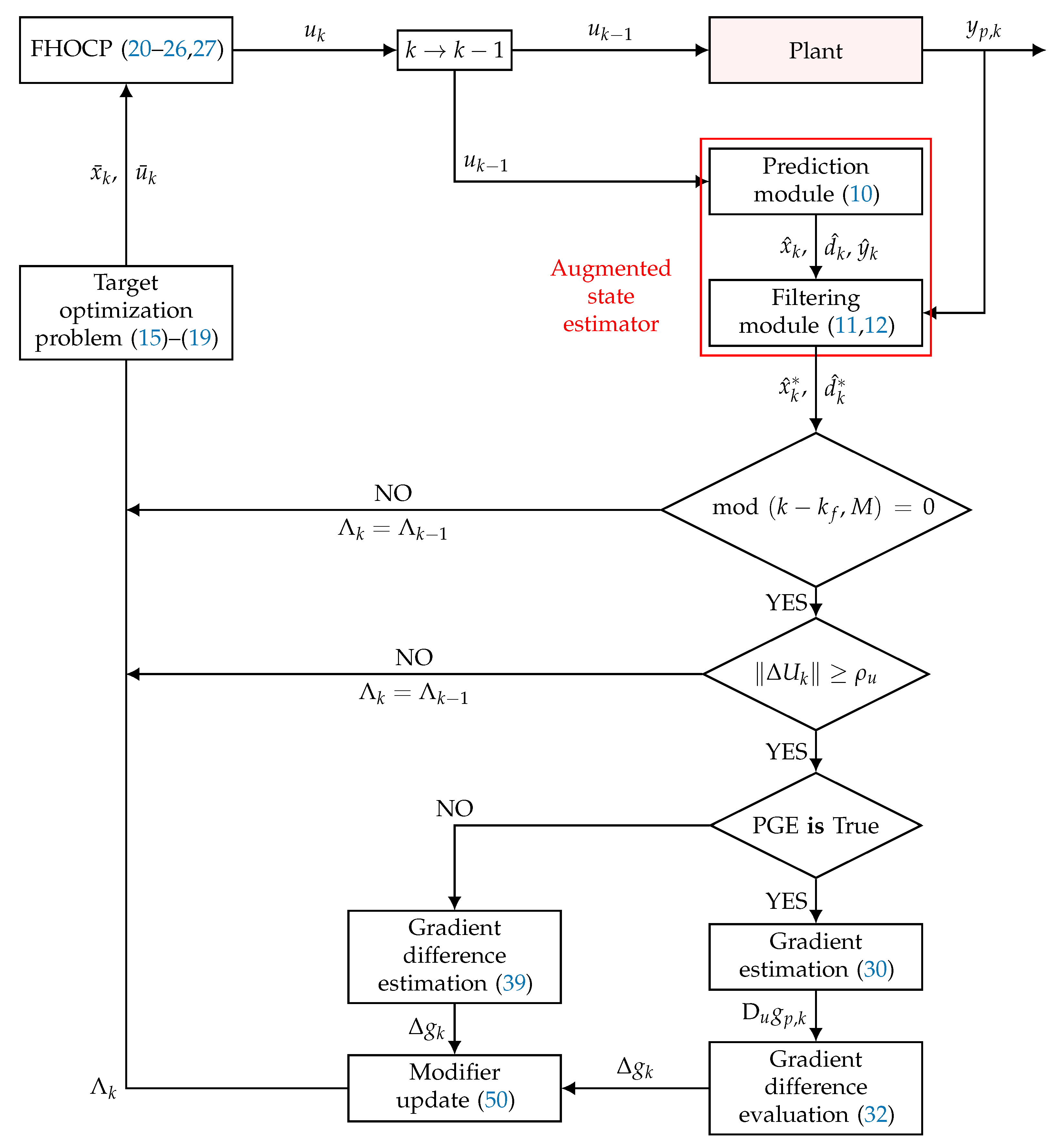
4. Offset-Free Economic MPC Algorithms

This sections formulates algorithmically the two OF-eMPC schemes based on Broyden’s update and linear regression. The way the algorithms are initialized is presented first.

4.1. Algorithm Initialization

To improve convergence speed, the OF-eMPC schemes require a good initial estimate for $\Delta g$, which translates into an appropriate ${\Lambda }_0$. This can be achieved by perturbing each input individually around the current operating point and calculating the corresponding gradient elements, which requires $n_u$ input perturbations. Following each perturbation, one must wait M sampling times for the system to approach a steady state.

Next, we detail this initialization phase. Let $k_0$ denote the iteration at which the plant first reaches steady state, with the inputs $u_{k_0}$. The following control law is then used during the initialization phase, for $j=1,\dots ,n_u$:

$$u_k=u_{k_0}+s_j{e}_j\mathrm{for}(j-1)M\le k-k_0<jM,$$

(45)

where $s_j$ is the amplitude of a step of duration M in the direction $e_j$, with $e_j$ being a unit vector in input space. One sees that the $j^{th}$ component of u is perturbed individually by the amount of $s_j{e}_j$ during M iterations. The initialization phase ends at iteration $k_f:=k_0+n_{u}M$.

The $j^{th}$ column of the plant gradient to be used in Equation (30) is estimated as

$${\mathrm{D}}_u{g}_{p,k_f,j}={\displaystyle \frac{y_{p,k_0+jM}-y_{p,k_0}}{s_j}},$$

(46)

while the $j^{th}$ column of the gradient differences to be used in Equation (39) is

$$\Delta g_{k_f,j}={\displaystyle \frac{(y_{p,k_0+jM}-y_{p,k_0})-\left(h\left({\widehat{x}}_{k_0+jM}\right)-h\left({\widehat{x}}_{k_0}\right)\right)}{s_j}}.$$

(47)

Note that, unlike Broyden’s update, the linear regression method in Equation (36) or in Equation (42) does not require Jacobian initialization, albeit the initialization phase is still used.

These estimated plant gradients or gradient differences are used to compute ${\Lambda }_k$ as follows:

$${\Lambda }_k=\{\begin{array}{cccc}0\hfill & \text{for} k_0<k<k_f\hfill & \text{(initialization phase)}\hfill & \text{(48)}\hfill \\ {\Lambda }_{k-1}\hfill & \text{if mod}\left(k-k_f,M\right)\ne 0\hfill & k>k_f\hfill & \text{(49)}\hfill \\ \left(1-\sigma \right){\Lambda }_{k-1}+\sigma \text{Δ}{g}_k\hfill & \text{if mod}\left(k-k_f,M\right)=0\hfill & k\ge k_f\hfill & \text{(50)}\hfill \end{array}$$

4.2. OF-eMPC Algorithm Using Broyden’s Update

The block diagram and algorithm describing the OF-eMPC scheme with Broyden’s update are given in Figure 1 and Algorithm 1. For the sake of brevity, the initialization phase is not shown, and only the behavior for $k>k_f$ is displayed.

As can be seen in Figure 1, gradient estimates are computed after $k_0+n_{u}M$ iterations. The modifier matrix is updated every M time steps, but only when the difference between two successive inputs is not too close to zero. This is needed to avoid calculating gradient differences based on little informative data, that is, to avoid ill-conditioning of the updating Equation (30) or Equation (39). Hence, the parameter ${\rho }_u$ can be seen as a tuning parameter for the performance of the gradient estimation method.

Algorithm 1 Offset-free eMPC algorithm using Broyden’s update.

1: Set $k=k_f$ and initialize $u_k$ using current plant values, ${\widehat{x}}_k^{*}$, ${\widehat{d}}_k^{*}$ from (12) and ${\Lambda }_k$ from (50), with ${\Lambda }_{k-1}=0$. 2: Inject inputs $u_k$ into plant and wait for next sampling instant. 3: Update time index $k:=k+1$. 4: Read $y_{p,k}$ from plant. 5: Predict successor quantities using (10). 6: Evaluate prediction errors using (11). 7: Estimate states and disturbances using (12). 8: if$mod(k-k_f,M)=0$then 9:     if Plant Gradient Estimation is True then 10:         Define $\Delta U_k$ and $\Delta Y_k$ as in (29) and (28). 11:     else 12:         Define $\Delta U_k$ and $\Delta E_k$ as in (29) and (38). 13:     end if 14:     if $∥\Delta U_k∥\ge {\rho }_u$ then 15:         if Plant Gradient Estimation is True then 16:            Evaluate plant gradients using (30). 17:            Evaluate gradient differences using (32). 18:         else 19:            Evaluate gradient differences using (39). 20:         end if 21:         Update modifier matrix using (50). 22:     else 23:         Do not update modifier matrix. 24:     end if 25: else 26:     Do not update modifier matrix. 27: end if 28: Solve (15)–(19) to obtain targets $\left({\overline{x}}_k,{\overline{u}}_k,{\overline{y}}_k\right)$. 29: Solve FHOCP (20)–(26), set inputs $u_k$ as per (27). 30: Output:$u_k$, ${\widehat{x}}_k^{*}$, ${\widehat{d}}_k^{*}$, and ${\Lambda }_k$. 31: Goto 2.

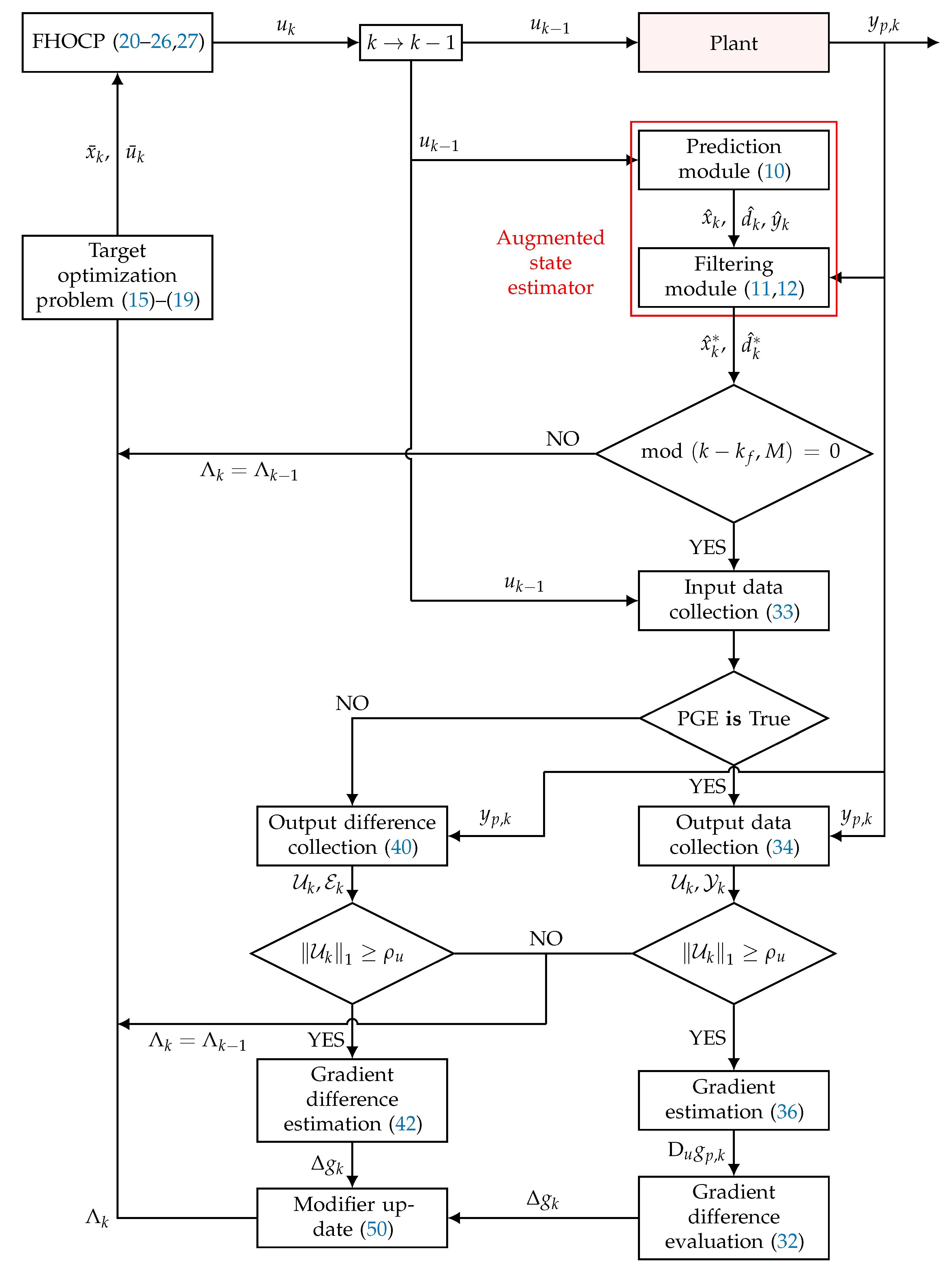
4.3. OF-eMPC Algorithm Using Linear Regression

The block diagram and algorithm describing the OF-eMPC scheme that uses linear regression are given in Figure 2 and Algorithm 2. Here, the initialization phase is not shown, and only the behavior for $k>k_f$ is displayed.

Algorithm 2 Offset-free eMPC algorithm using linear regression

1: Set $k=k_f$ and initialize $u_k$ using current plant values, ${\widehat{x}}_k^{*}$, ${\widehat{d}}_k^{*}$ from (12) and ${\Lambda }_k$ from (50), with ${\Lambda }_{k-1}=0$. 2: Inject inputs $u_k$ into plant and wait for next sampling instant. 3: Update time index $k:=k+1$. 4: Read $y_{p,k}$ from plant. 5: Predict successor quantities using (10). 6: Evaluate prediction errors using (11). 7: Estimate states and disturbances using (12). 8: if$mod(k-k_f,M)=0$ then 9:      Update input matrix ${\mathcal{U}}_k$ as in (33). 10:     if Plant gradient estimation is True then 11:         Update output matrix ${\mathcal{Y}}_k$ as in (34). 12:     else 13:         Update output difference matrix ${\mathcal{E}}_k$ as in (40). 14:     end if 15:         if ${∥{\mathcal{U}}_k∥}_1\ge {\rho }_u$ then 16:            if Plant gradient estimation is True then 17:                Evaluate plant gradients using (36) 18:                Evaluate gradient differences using (32). 19:            else 20:                Evaluate gradient differences using (42). 21:            end if 22:            Update modifier matrix using (50). 23:         else 24:            Do not update modifier matrix. 25:         end if 26:     else 27:         Do not update modifier matrix. 28:     end if 29:     Solve (15)–(19) to obtain targets $\left({\overline{x}}_k,{\overline{u}}_k,{\overline{y}}_k\right)$. 30:     Solve FHOCP (20)–(26), set inputs $u_k$ as in (27). 31:     Output: $u_k$, ${\widehat{x}}_k^{*}$, ${\widehat{d}}_k^{*}$, and ${\Lambda }_k$. 32:     Goto 2.

4.4. Ill-Conditioning

Ill-conditioning of $\Delta g_k$ in Equations (30), (36), (39), or (36) results from too small a value of $\Delta U_k$ or ${\mathcal{U}}_k$. When $\Delta U_k$ or ${\mathcal{U}}_k$ tends to zero, the aforementioned $\Delta g_k$ can no longer be calculated. This happens when two measurements corresponding to (almost) the same steady state are used in $\Delta U_k$ or ${\mathcal{U}}_k$, that is, with $u_{k-1}\approxeq u_{k-M-1}$. Hence, before calculating $\Delta g_k$, we compare the value of $\Delta U_k$ or ${\mathcal{U}}_k$ with the threshold value ${\rho }_u$, which depends on the input–output sensitivity and the size of measurement noise. This is an engineering choice that the designer has to make based on the process at hand.

We underline that, if modifier update does not take place due to ill-conditioning, and thus the previous values of the gradients or modifiers are used, Problems (15) and (20) are still solved as part of OF-eMPC. On the other hand, if the inputs u get “stuck” far away from plant optimality, the system requires additional excitation for accurate estimation of plant gradients or modifiers.

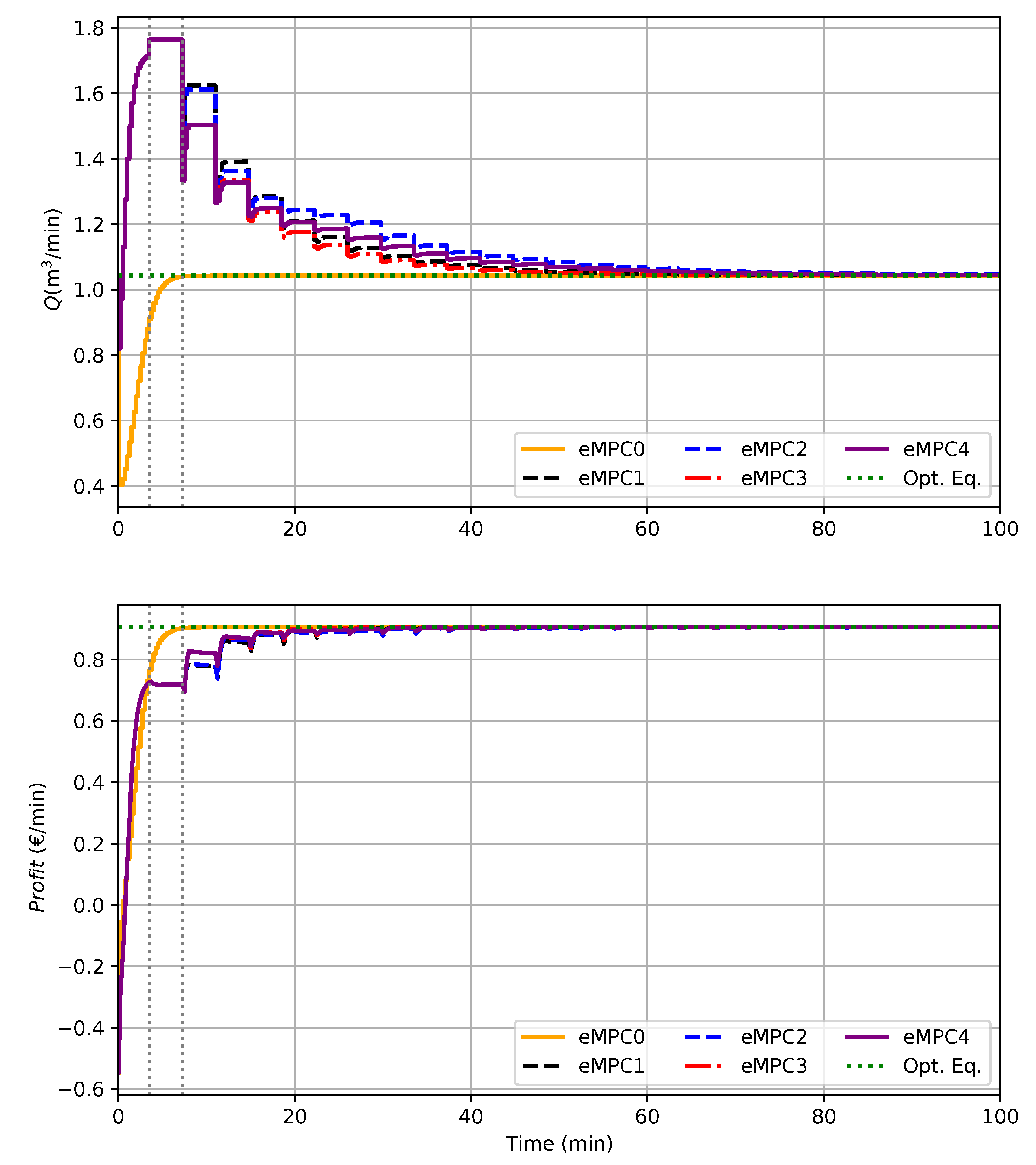
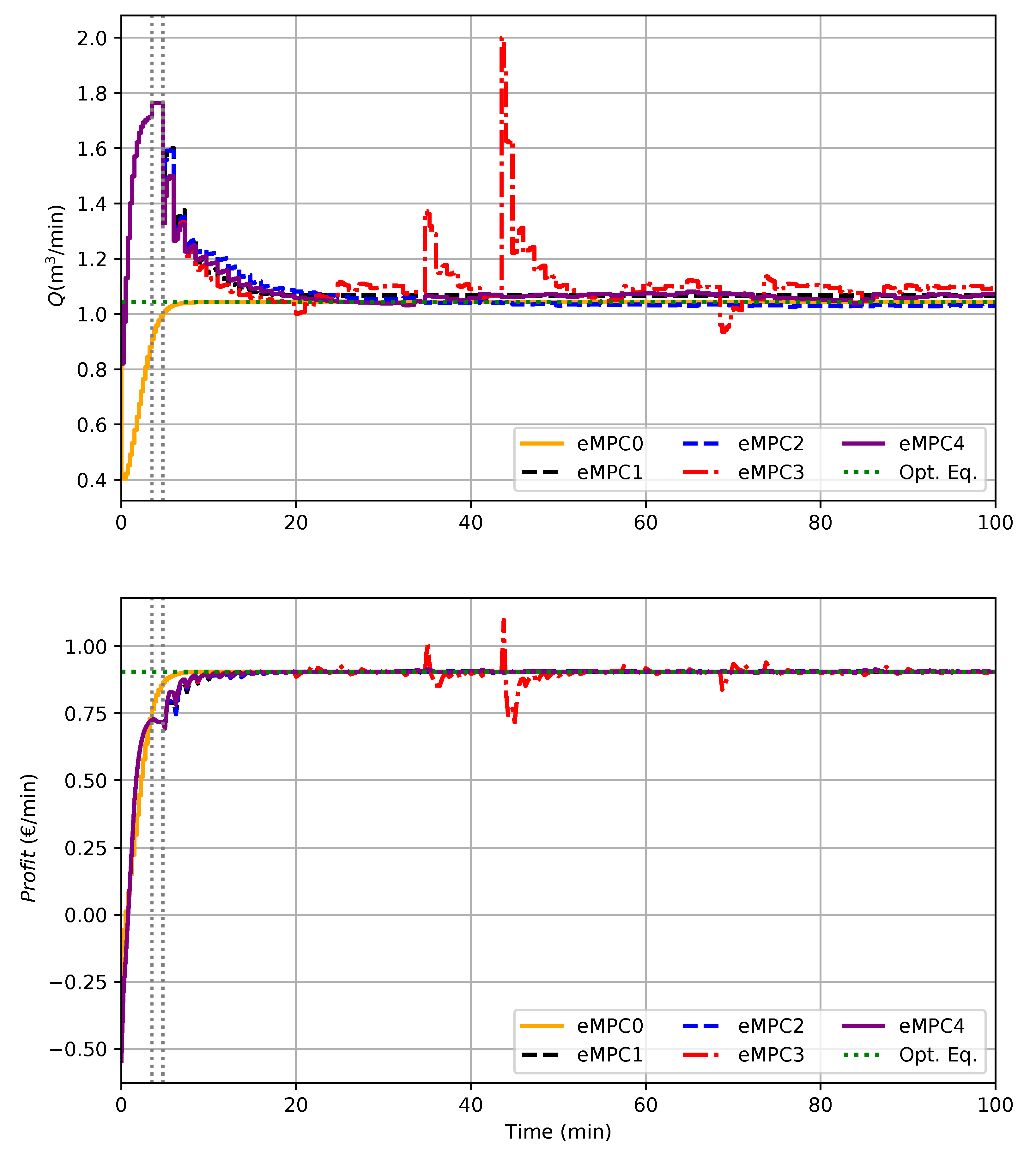
5. Simulation Results

Two examples taken from the literature are used to compare the performance of five eMPC schemes, all using the same nominal model, cost function, and sampling time. There is significant plant–model mismatch, and the augmented model (9) reads

$$\begin{array}{cc}{x}^{+}\hfill & =f(x,u)\hfill \\ d^{+}\hfill & =d\hfill \\ y\hfill & =h\left(x\right)+d.\hfill \end{array}$$

(51)

The estimator of Section 2.3 is the deadbeat Kalman filter with the parameters $K_x=\mathbf{0}$ and $K_d=\mathrm{I}$. In addition, all eMPC controllers use the target calculation (15) and the FHOCP (20). The five controllers are the following:

• eMPC0 assumes the plant gradients to be perfectly known, i.e., ${\mathrm{D}}_u{g}_{p,k}={\mathrm{D}}_u{g}_p\left({\overline{u}}_{k-1}\right)$. This controller is not practically implementable but is used as reference.
• eMPC1 uses the Broyden’s gradient update described in Section 3.2.1.
• eMPC2 estimates the plant gradient using linear regression as per Section 3.2.2. The number of data points in the regression is $n_s=4$.
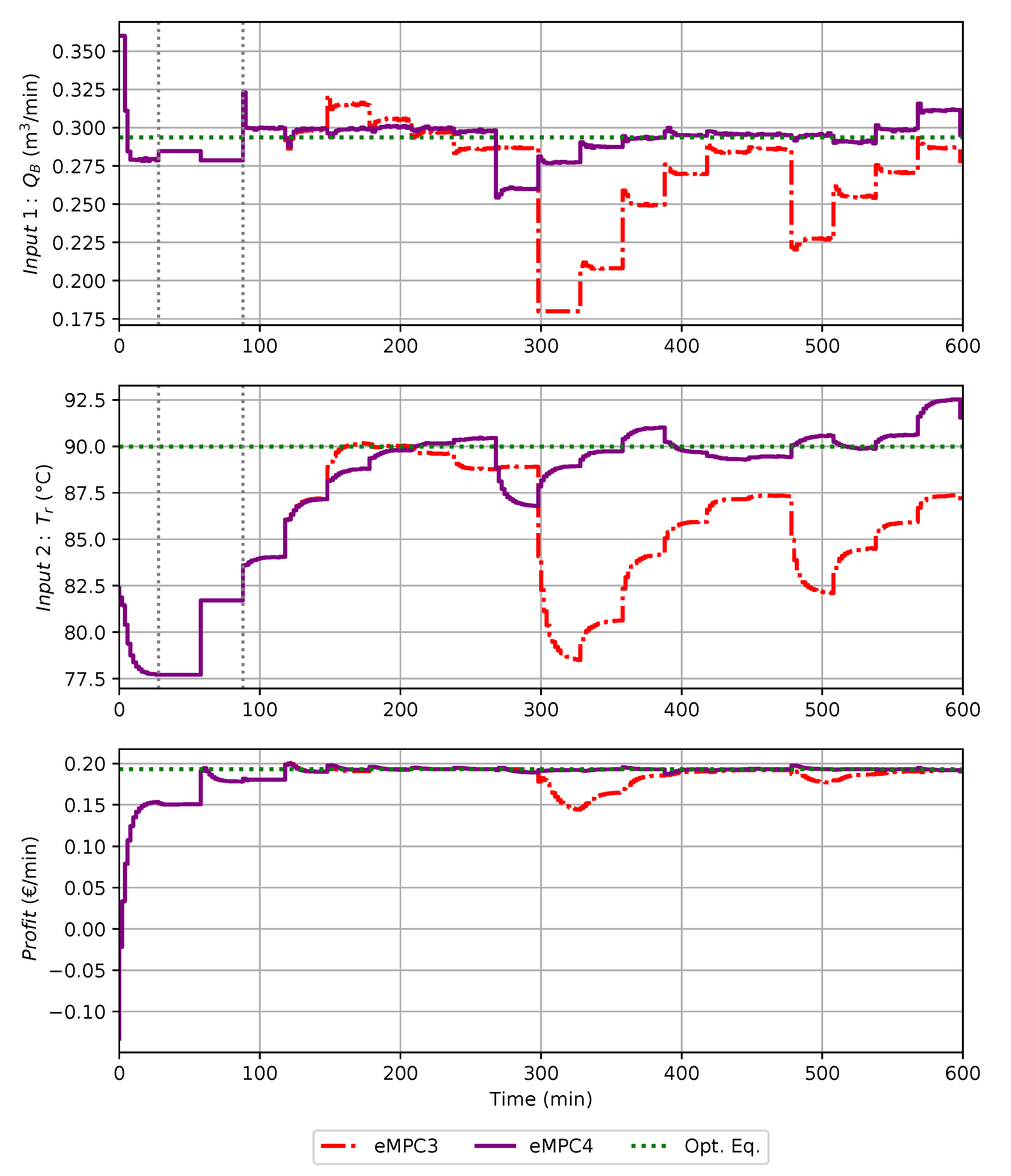
• eMPC3 uses the Broyden’s modifier update described in Section 3.3.1.
• eMPC4 estimates the modifiers using linear regression as per Section 3.3.2. The number of data points in the regression is also $n_s=4$.

Note that, in the presence of plant–model mismatch, the use of the disturbance model (51) by itself is not sufficient to eliminate offset, as reaching plant optimality requires perfect knowledge of plant gradients [25,32]. When not otherwise specified, $M=15$ is chosen for all controllers. Moreover, the filter constant for updating the modifiers in Equation (13) is $\sigma =0.5$, and the tolerance threshold for avoiding numerical ill-conditioning is ${\rho }_u=5·{10}^{-4}$.

5.1. CSTR with Competitive Reactions

The first example is a continuous stirred-tank reactor (CSTR), in which two consecutive reactions take place:

$$\begin{array}{c}\hfill A\stackrel{k_1}{\to }B\stackrel{k_2}{\to }C.\end{array}$$

(52)

The objective is to maximize the profit expressed as the difference between the revenues generated by the desired product B and the cost of the raw material A. The following system of ordinary differential equations describes the reactor dynamics:

$$\begin{array}{cc}{\dot{x}}_1\hfill & =\frac{u}{V}(c_{A0}-x_1)-k_1{x}_1\hfill \\ {\dot{x}}_2\hfill & =\frac{u}{V}(c_{B0}-x_2)+k_1{x}_1-k_2{x}_2,\hfill \end{array}$$

(53)

where $x_1$ and $x_2$ represent the molar concentrations of A and B in the reactor, the corresponding feed concentrations are $c_{A0}$ and $c_{B0}$, and the input u is the feed flow rate regulated through a valve. For the sake of simplicity, the reactor is assumed to have a constant volume V and to be isothermal. Both states are assumed to be measured. The reactor parameters are taken from [25]. Optimal steady-state performance is computed by solving the following optimization problem:

$$\begin{array}{c}\underset{u,x}{max}p(u,x)\end{array}$$

(54)

subject to

$$\begin{array}{c}\hfill \frac{u}{V}(c_{A0}-x_1)-k_1{x}_1=0\end{array}$$

(55)

$$\begin{array}{c}\hfill \frac{u}{V}(c_{B0}-x_2)+k_1{x}_1-k_2{x}_2=0\end{array}$$

(56)

$$\begin{array}{c}\hfill 0\le x_1\le c_{A0}\end{array}$$

(57)

$$\begin{array}{c}\hfill 0\le x_2\le c_{A0},\end{array}$$

(58)

with the running profit

$$p(u,x)={\beta }_{B}u{x}_2-{\beta }_{A}u{c}_{A0}.$$

(59)

Optimal operation corresponds to $u_s^{*}=1.043{\mathrm{m}}^3/\min$, $x_{1,s}^{*}=0.511\mathrm{kmol}/{\mathrm{m}}^3$, and $x_{2,s}^{*}=0.467\mathrm{kmol}/{\mathrm{m}}^3$ with the maximal profit $p(u^{*},x^{*})=0.906/\min$.

5.1.1. Model

We assume plant–model mismatch and design the controller with erroneous values of the two kinetic parameters: the model values known by the controller are ${\tilde{k}}_1=0.5{\min }^{-1}$ and ${\tilde{k}}_2=0.4{\min }^{-1}$, meaning that, compared to the true values $k_1=1.0{\min }^{-1}$ and $k_2=0.05{\min }^{-1}$, the first reaction rate is underestimated, while the second one is overestimated. The economic cost function to be minimized in Problem (20) is

$$\begin{array}{c}\hfill {\ell }_e(y\left(t_i\right),u\left(t_i\right))=-{\int }_{t_i}^{t_i+\tau }p\left(u\left(t\right),y_2\left(t\right)\right)dt={\int }_{t_i}^{t_i+\tau }\left[{\beta }_{A}u\left(t\right)c_{A0}-{\beta }_{B}u\left(t\right)y_2\left(t\right)\right]dt,\end{array}$$

(60)

with the sampling time $\tau =0.25\min$. Furthermore, the dynamics (53) is discretized using an implicit Euler method and the initial conditions are $x_{1,0}=x_{2,0}=0.1\mathrm{kmol}/{\mathrm{m}}^3$. Note that, with ${\tau }_{st}\simeq 4min$, the choice $M=15$ is quite appropriate.

5.1.2. Reactor Performance

The input and the cost function of the reactor with the five aforementioned controllers are depicted in Figure 3. We can immediately see that all schemes reach plant optimality even under the presence of plant–model mismatch. Before reaching the initialization phase at $t=3.75min$, the behavior is the same for the practical controllers eMPC1–eMPC4 as they all use the disturbance model (51) and no first-order correction. eMPC0 is, of course, significantly better as it uses perfect knowledge of plant gradients. ${\Lambda }_k$ is updated for the first time at time step $k_f=k_0+n_{u}M=30$, which corresponds to $t=7.5min$. After initialization, we see a slight difference between the schemes that use Broyden’s update (eMPC1 and eMPC3) and those that rely on linear regression (eMPC2 and eMPC4). All of them start to move towards plant optimality, with the methodologies using Broyden’s update reaching steady state faster. We observe a steplike profile, since the corrections are updated every M time samples. The average convergence time for the proposed methods is about 40$min$.

To speed up convergence, one can reduce the value of M, thereby looking for a compromise between convergence speed and steadiness of the collected samples. Figure 4 shows the reactor performance with the five controllers when M has been reduced from 15 to 5. For the sake of comparison, the same initial steady state was used, that is, we have $k_0=15$ and $k_f=20$, with $t=5min$ being the first time that ${\Lambda }_k$ is updated. All schemes reach plant optimality in about half the time of the previous case. Note also that, with all schemes, the profit (bottom panel of Figure 4) quickly reaches plant optimality. Only eMPC3 presents some erratic behavior that could result from poor numerical conditioning when Broyden’s update is used on the gradient difference. However, adjusting the filtering parameter $\alpha$ can improve the situation.

5.2. Williams–Otto Reactor

5.2.1. Process

As a well-known RTO example [10,44], the Williams–Otto reactor is a nonisothermal CSTR, in which three reactions take place:

$$\begin{array}{ccc}\mathrm{A}+\mathrm{B}& \stackrel{k_1}{\to }\mathrm{C}& r_1=k_1\left(T_r\right)c_{\mathrm{A}}{c}_{\mathrm{B}}\\ \mathrm{B}+\mathrm{C}& \stackrel{k_2}{\to }\mathrm{P}+\mathrm{E}& r_2=k_2\left(T_r\right)c_{\mathrm{B}}{c}_{\mathrm{C}}\\ \mathrm{C}+\mathrm{P}& \stackrel{k_3}{\to }\mathrm{G}& r_3=k_3\left(T_r\right)c_C{c}_{\mathrm{P}}.\end{array}$$

(61)

The reactor feed consists of two components: Species A fed at the constant flow rate $Q_{\mathrm{A}}$ with molar concentration $c_{\mathrm{A}0}$, and Species $\mathrm{B}$ added at the variable flow rate $Q_{\mathrm{B}}$ with molar concentration $c_{\mathrm{B}0}$. The desired products are $\mathrm{P}$ and $\mathrm{E}$, while $\mathrm{C}$ and $\mathrm{G}$ are intermediate and undesired products, respectively. The reactor outlet flow rate $Q_r$ is set equal to the sum of the two inlet flow rates, that is, $Q_r=Q_{\mathrm{A}}+Q_{\mathrm{B}}$, with the reactor volume V being constant. Mimicking realistic process conditions, only the molar concentrations of the two desired products are assumed to be measured, that is, $y_p={\left[\begin{array}{cc}{c}_{\mathrm{P}}& c_{\mathrm{E}}\end{array}\right]}^T$. The reactor temperature $T_r$ is manipulated, assuming ideal cooling. The kinetic parameters depend on the reactor temperature via an Arrhenius-type law:

$$k_i\left(T_r\right)=k_{i0}exp\left({\displaystyle \frac{-E_i}{T_r+273.15}}\right)\mathrm{for}i=1,2,3.$$

(62)

For the sake of brevity, the system dynamics are not reported here but can be found in [12]. The reactor has two inputs, namely, the temperature $T_r$ and the flow rate $Q_{\mathrm{B}}$. The profit to be maximized is

$$p(·)=Q_r{c}_{\mathrm{P}}{p}_{\mathrm{P}}+Q_r{c}_{\mathrm{E}}{p}_{\mathrm{E}}-Q_{\mathrm{A}}{c}_{\mathrm{A}0}{p}_{\mathrm{A}}-Q_{\mathrm{B}}{c}_{\mathrm{B}0}{p}_{\mathrm{B}},$$

(63)

where $p_{\mathrm{P}},p_{\mathrm{E}},p_{\mathrm{A}},$ and $p_{\mathrm{B}}$ are the molar prices of products and reactants. The plant parameters can be found in [32] and in

Table 1. William–Otto reactor: Plant parameters.

Parameter	Value	Unit
$k_{10}$	$9.9594\times {10}^6$	${\mathrm{m}}^3/(\mathrm{kmol}·\min )$
$k_{20}$	$8.66124\times {10}^9$	${\mathrm{m}}^3/(\mathrm{kmol}·\min )$
$k_{30}$	$9.9594\times {10}^6$	${\mathrm{m}}^3/(\mathrm{kmol}·\min )$
$E_1$	$6666.7$	$\mathrm{K}$
$E_2$	$8333.3$	$\mathrm{K}$
$E_3$	11,111	$\mathrm{K}$
$c_{\mathrm{A}0}$	10	$\mathrm{kmol}/{\mathrm{m}}^3$
$c_{\mathrm{B}0}$	10	$\mathrm{kmol}/{\mathrm{m}}^3$
V	$2.105$	${\mathrm{m}}^3$
$Q_{\mathrm{A}}$	$112.35$	${\mathrm{m}}^3/\min$
$p_{\mathrm{A}}$	$7.623$	$\$/\mathrm{kmol}$
$p_{\mathrm{B}}$	$11.434$	$\$/\mathrm{kmol}$
$p_{\mathrm{P}}$	$114.338$	$\$/\mathrm{kmol}$
$p_{\mathrm{E}}$	$5.184$	$\$/\mathrm{kmol}$

.

5.2.2. Model

The model used for control design comprises only two reactions:

$$\begin{array}{ccc}\mathrm{A}+2\mathrm{B}& \stackrel{{\tilde{k}}_1}{\to }\mathrm{P}+\mathrm{E}& {\tilde{r}}_1={\tilde{k}}_1\left(T_r\right)c_{\mathrm{A}}{c}_{\mathrm{B}}^2\\ \mathrm{A}+\mathrm{B}+\mathrm{P}& \stackrel{{\tilde{k}}_2}{\to }\mathrm{G}& {\tilde{r}}_2={\tilde{k}}_2\left(T_r\right)c_{\mathrm{A}}{c}_{\mathrm{B}}{c}_{\mathrm{P},}\end{array}$$

(64)

for which the kinetic parameters are reported in

Table 2. Williams–Otto reactor: Model parameters.

Parameter	Value	Unit
${\tilde{k}}_{10}$	$1.3134\times {10}^8$	${\mathrm{m}}^6/\left({\mathrm{kmol}}^2·\min \right)$
${\tilde{k}}_{20}$	$2.586\times {10}^{13}$	${\mathrm{m}}^6/\left({\mathrm{kmol}}^2·\min \right)$
${\tilde{E}}_1$	$8077.6$	$\mathrm{K}$
${\tilde{E}}_2$	12,438.5	$\mathrm{K}$

.

We can infer from Equation (64) that they are 5 model states,

$$x={\left[\begin{array}{ccccc}{c}_{\mathrm{A}}& c_{\mathrm{B}}& c_{\mathrm{P}}& c_{\mathrm{E}}& c_G\end{array}\right]}^T,$$

while the plant has 6 states,

$$x_p={\left[\begin{array}{cccccc}{c}_{\mathrm{A}}& c_{\mathrm{B}}& c_{\mathrm{C}}& c_{\mathrm{P}}& c_{\mathrm{E}}& c_{\mathrm{G}}\end{array}\right]}^T.$$

In addition, the inputs are bounded as follows:

$$\begin{array}{cc}\hfill {0.18\mathrm{m}}^3/\min & \le Q_{\mathrm{B}}\le {0.36\mathrm{m}}^3/\min \hfill \end{array}$$

(65)

$$\begin{array}{cc}\hfill 75°\mathrm{C}& \le T_{\mathrm{r}}\le 100°\mathrm{C}.\hfill \end{array}$$

(66)

5.2.3. Reactor Optimization

The sampling time in this example is $\tau =2$ min, which calls for $M\tau =30$ min between two successive modifier updates. In this case, with ${\tau }_{st}=35min$, the choice $M=15$ is also quite appropriate. The performance of the five controllers is depicted in Figure 5, together with the optimal operating point that is unknown to the controllers. $\Lambda$-initialization is performed in the time interval of 30–90 min. The starting point for the model state vector is

$$x_0={\left[\begin{array}{ccccc}2& 2& 1.1& 1& 0.6\end{array}\right]}^T,$$

and the first measurement from the plant reads $y_{p,0}={\left[\begin{array}{cc}1.1& 0.6\end{array}\right]}^T$.

A behavior similar to that shown in Figure 3 can be observed, namely, (i) all schemes reach plant optimality; (ii) before the initialization phase, the practical schemes eMPC1-4 behave alike since the modifier matrix is still zero. Then, from $k_0\tau =30$ to $k_f\tau =90$ min, the two inputs are excited individually and sequentially as described in Section 4.1. Once a nonzero modifier matrix has been computed, we see a difference between the schemes that use plant-gradient estimation (eMPC1 and eMPC2) and those that estimate the gradient differences directly (eMPC3 and eMPC4). In this example, the schemes that rely on plant-gradient estimation do not work well: eMPC1 and eMPC2 fail to reach plant optimality; in addition, eMPC2 converges slowly, while the second input with eMPC1 gets stuck to its upper bound. In contrast, eMPC3 and eMPC4 are able to reach plant optimality. These results indicate that the two schemes based on estimating the gradient differences give the best performance.

In order to check the robustness of these last two schemes, we propose to corrupt the measurements with white noise, i.e., Plant (1) is modified as follows:

$$\begin{array}{cc}\hfill x_p^{+}& =f_p(x_p,u)\\ \hfill y_p& =h_p\left(x_p\right)+R_{v}v,\end{array}$$

(67)

where $v\in {\mathbb{R}}^{n_y}$ is a white noise signal with covariance $R_v={10}^{-3}{\mathrm{I}}_{n_y}$. Figure 6 shows the effect of noise on the convergence performance of eMPC3 and eMPC4. It is seen that linear regression handles measurement noise better than Broyden’s update since the former uses measurements stemming from several measurement points and therefore possesses a stronger filtering effect. Note that eMPC3 and eMPC4 perform very similarly right after the initialization phase when the number of measurements points is the same. As shown in the top panels of Figure 6, as time advances and more measurements become available to eMPC4, the inputs are able to move much quicker than with eMPC3. Another illustration of the improved resilience of eMPC4 with respect to measurement noise is shown by the profit profile in the bottom panel of Figure 6.

5.3. Final Considerations

An interesting result is the improvement in estimation quality when the modifiers are estimated directly rather than computed from the estimated plant gradients and the predicted model gradients. This is related to the nature of the estimation error. The gradient estimation error encompasses two terms resulting from truncation error and measurement noise, respectively (see [9] for a more comprehensive discussion). These two error types are quite different in nature, with the former being systematic and the latter being random. On this basis, one can consider two different ways of estimating the modifiers:

• Estimate the plant gradients from measurements, compute the model gradients “analytically” from the model, and evaluate the modifiers as their differences, as per Section 3.2. This approach is very sensitive to truncation errors, as these errors affect the estimation of plant gradients but not of model gradients.
• Estimate the plant gradients from measurements, estimate the model gradients from the model using the same numerical scheme, and evaluate the modifiers as their differences. This is equivalent to estimating the modifiers directly from measurements (see Section 3.3). In this case, the truncation errors tend to cancel out upon computing the differences between plant and model gradients.

6. Conclusions

Different offset-free economic model predictive control schemes that combine an augmented model structure and first-order modifiers on the outputs have been proposed in recent years. These schemes proved to converge asymptotically to plant optimality, even under plant–model mismatch. The main caveat of this formulation is the requirement of perfect knowledge of static plant gradients.

This paper has investigated two different techniques to estimate plant gradients using steady-state measurements, namely, Broyden’s update and linear regression. These techniques have been adapted and applied to estimate either the plant gradient or the modifiers directly. Consequently, four different approaches have been tested via two examples: in the first (single-input) example, all methods give satisfactory results, and also when the time between modifier updates is reduced to boost convergence speed. In the second (multi-input) example, only the approach that estimates the modifiers directly succeeded in reaching plant optimality. The approach was tested using both Broyden’s update and linear regression. It was found that the approach that uses linear regression is clearly superior in handling measurement noise. In general, although the most effective estimation method should be chosen according to the specific case, it appears from these results that estimating the modifiers directly is more effective than estimating the plant gradient alone. Furthermore, in the presence of measurement noise, modifier estimation is best implemented via linear regression.

Note that these findings are not the end of the story, as this investigation was limited to plant gradient estimation using as many steady-state measurements as possible ($M=15$ in this study). As mentioned in the introduction, one would like to be able to estimate static plant gradients using transient data, so as to speed up convergence even more (ideally, $M=1$). Hence, a similar type of study to analyze the performance of eMPC in the presence of plant–model mismatch and the availability of transient measurements is very welcome. Finally, in the present paper, closed-loop stability has been assumed as per Assumption 5. However, the stability of eMPC under plant–model mismatch is still an open issue, which may motivate future research.

References

1. Rawlings, J.B.; Angeli, D.; Bates, C.N. Fundamentals of economic model predictive control. In Proceedings of the 51st IEEE Conference on Decision and Control, Maui, HI, USA, 10–13 December 2012; pp. 3851–3861. [Google Scholar]
2. Morari, M.; Arkun, Y.; Stephanopoulos, G. Studies in the synthesis of control structures for chemical processes: Part I: Formulation of the problem. Process decomposition and the classification of the control tasks. Analysis of the optimizing control structures. AIChE J. 1980, 26, 220–232. [Google Scholar] [CrossRef]
3. Engell, S. Feedback control for optimal process operation. J. Process Control 2007, 17, 203–219. [Google Scholar] [CrossRef]
4. Ellis, M.; Christofides, P.D. On finite-time and infinite-time cost improvement of economic model predictive control for nonlinear systems. Automatica 2014, 50, 2561–2569. [Google Scholar] [CrossRef]
5. Pannocchia, G.; Rawlings, J.B. Disturbance models for offset-free model-predictive control. AIChE J. 2003, 49, 426–437. [Google Scholar] [CrossRef]
6. Muske, K.R.; Badgwell, T.A. Disturbance modeling for offset-free linear model predictive control. J. Process Control 2002, 12, 617–632. [Google Scholar] [CrossRef]
7. Pannocchia, G. Offset-free tracking MPC: A tutorial review and comparison of different formulations. In Proceedings of the European Control Conference, Linz, Austria, 15–17 July 2015; pp. 527–532. [Google Scholar]
8. Marchetti, A.G.; Chachuat, B.; Bonvin, D. Modifier-adaptation methodology for real-time optimization. Ind. Eng. Chem. Res. 2009, 48, 6022–6033. [Google Scholar] [CrossRef] [Green Version]
9. Marchetti, A.G.; Chachuat, B.; Bonvin, D. A dual modifier-adaptation approach for real-time optimization. J. Process Control 2010, 20, 1027–1037. [Google Scholar] [CrossRef] [Green Version]
10. Marchetti, A.; François, G.; Faulwasser, T.; Bonvin, D. Modifier adaptation for real-time optimization—Methods and applications. Processes 2016, 4, 55. [Google Scholar] [CrossRef] [Green Version]
11. Vaccari, M.; Pannocchia, G. A Modifier-Adaptation Strategy towards Offset-Free Economic MPC. Processes 2016, 5, 2. [Google Scholar] [CrossRef] [Green Version]
12. Faulwasser, T.; Pannocchia, G. Towards a unifying framework blending RTO and economic MPC. Ind. Eng. Chem. Res. 2019, 58, 13583–13598. [Google Scholar] [CrossRef]
13. Vergara-Diertrich, J.; Ferramosca, A.; Mirasierra, V.; Normey-Rico, J.E.; Limon, D. A Modifier-Adaptation Approach to the One-Layer Economic MPC. IFAC-PapersOnLine 2020, 53, 6957–6962. [Google Scholar] [CrossRef]
14. Papasavvas, A.; de Avila Ferreira, T.; Marchetti, A.G.; Bonvin, D. Analysis of output modifier adaptation for real-time optimization. Comput. Chem. Eng. 2019, 121, 285–293. [Google Scholar] [CrossRef]
15. Marchetti, A.G.; Faulwasser, T.; Bonvin, D. A feasible-side globally convergent modifier-adaptation scheme. J. Process Control 2017, 54, 38–46. [Google Scholar] [CrossRef]
16. Schneider, R.; Milosavljevic, P.; Bonvin, D. Accelerated and adaptive modifier-adaptation schemes for the real-time optimization of uncertain systems. J. Process Control 2019, 83, 129–135. [Google Scholar] [CrossRef]
17. Mirasierra, V.; Vergara-Diertrich, J.; Limon, D. Real-Time Optimization of Periodic Systems: A Modifier-Adaptation Approach. IFAC-PapersOnLine 2020, 53, 1690–1695. [Google Scholar] [CrossRef]
18. Papasavvas, A.; Francois, G. Internal Modifier Adaptation for the Optimization of Large-Scale Plants with Inaccurate Models. Ind. Eng. Chem. Res. 2019, 58, 13568–13582. [Google Scholar] [CrossRef]
19. Gao, W.; Wenzel, S.; Engell, S. Modifier adaptation with quadratic approximation in iterative optimizing control. In Proceedings of the European Control Conference, Linz, Austria, 15–17 July 2015; pp. 2527–2532. [Google Scholar]
20. Costello, S.; François, G.; Bonvin, D. A Directional Modifier-Adaptation Algorithm for Real-Time Optimization. J. Process Control 2016, 39, 64–76. [Google Scholar] [CrossRef] [Green Version]
21. Pannocchia, G. An economic MPC formulation with offset-free asymptotic performance. IFAC-PapersOnLine 2018, 51, 393–398. [Google Scholar] [CrossRef]
22. François, G.; Bonvin, D. Use of transient measurements for the optimization of steady-state performance via modifier adaptation. Ind. Eng. Chem. Res. 2013, 53, 5148–5159. [Google Scholar] [CrossRef] [Green Version]
23. de Avila Ferreira, T.; François, G.; Marchetti, A.G.; Bonvin, D. Use of transient measurements for static real-time optimization. IFAC-PapersOnLine 2017, 50, 5737–5742. [Google Scholar] [CrossRef]
24. Hernández, R.; Engell, S. Economics Optimizing Control with Model Mismatch Based on Modifier Adaptation. IFAC-PapersOnLine 2019, 52, 46–51. [Google Scholar] [CrossRef]
25. Vaccari, M.; Pannocchia, G. Implementation of an economic MPC with robustly optimal steady-state behavior. IFAC-PapersOnLine 2018, 51, 92–97. [Google Scholar] [CrossRef]
26. Singhal, M.; Marchetti, A.G.; Faulwasser, T.; Bonvin, D. Active directional modifier adaptation for real-time optimization. Comput. Chem. Eng. 2018, 115, 246–261. [Google Scholar] [CrossRef]
27. Marchetti, A.; de Avila Ferreira, T.; Costello, S.; Bonvin, D. Modifier adaptation as a feedback control scheme. Ind. Eng. Chem. Res. 2020, 59, 2261–2274. [Google Scholar] [CrossRef]
28. Singhal, M.; Marchetti, A.G.; Faulwasser, T.; Bonvin, D. A note on efficient computation of privileged directions in modifier adaptation. Comput. Chem. Eng. 2020, 132, 106524. [Google Scholar] [CrossRef]
29. Jeong, D.H.; Lee, C.J.; Lee, J.M. Experimental gradient estimation of multivariable systems with correlation by various regression methods and its application to modifier adaptation. J. Process Control 2018, 70, 65–79. [Google Scholar] [CrossRef]
30. Navia, D.; Briceño, L.; Gutiérrez, G.; De Prada, C. Modifier-Adaptation Methodology for Real-Time Optimization Reformulated as a Nested Optimization Problem. Ind. Eng. Chem. Res. 2015, 54, 12054–12071. [Google Scholar] [CrossRef]
31. Oliveira-Silva, E.; de Prada, C.; Navia, D. Dynamic optimization integrating modifier adaptation using transient measurements. Comput. Chem. Eng. 2021, 149, 107282. [Google Scholar] [CrossRef]
32. Vaccari, M.; Pelagagge, F.; Dominique, B.; Pannocchia, G. Estimation technique for offset-free economic MPC based on modifier adaptation. IFAC-PapersOnLine 2020, 53, 11251–11256. [Google Scholar] [CrossRef]
33. Maeder, U.; Borrelli, F.; Morari, M. Linear offset-free model predictive control. Automatica 2009, 45, 2214–2222. [Google Scholar] [CrossRef]
34. Morari, M.; Maeder, U. Nonlinear offset-free model predictive control. Automatica 2012, 48, 2059–2067. [Google Scholar] [CrossRef]
35. Pannocchia, G.; Gabiccini, M.; Artoni, A. Offset-free MPC explained: Novelties, subtleties, and applications. IFAC-PapersOnLine 2015, 48, 342–351. [Google Scholar] [CrossRef]
36. Rawlings, J.B.; Allan, D.A. Moving horizon estimation. Encycl. Syst. Control 2020, 1–7. [Google Scholar] [CrossRef]
37. Angeli, D.; Amrit, R.; Rawlings, J.B. On average performance and stability of economic model predictive control. IEEE Trans. Autom. Control 2012, 57, 1615–1626. [Google Scholar] [CrossRef] [Green Version]
38. Vaccari, M.; Pannocchia, G. A performance monitoring algorithm for sustained optimal operation with economic MPC. In Proceedings of the 2019 18th European Control Conference (ECC), Naples, Italy, 25–28 June 2019; pp. 3353–3358. [Google Scholar]
39. Roberts, P.D. Broyden derivative approximation in ISOPE optimising and optimal control algorithms. In Proceedings of the 11th IFAC Workshop on Control Applications of Optimisation, Saint Petersburg, Russia, 3–6 July 2000; pp. 283–288. [Google Scholar]
40. Rodger, E.A.; Chachuat, B. Design methodology of modifier adaptation for on-line optimization of uncertain processes. In Proceedings of the IFAC World Congress, Milan, Italy, 28 August–2 September 2011; pp. 4113–4118. [Google Scholar]
41. Dennis, J.E., Jr.; Schnabel, R.B. Numerical Methods for Unconstrained Optimization and Nonlinear Equations; SIAM: Philadelphia, PA, USA, 1996; Volume 16. [Google Scholar]
42. Kelley, C.T. Iterative Methods for Optimization; SIAM: Philadelphia, PA, USA, 1999. [Google Scholar]
43. Marchetti, A.G. A new dual modifier-adaptation approach for iterative process optimization with inaccurate models. Comput. Chem. Eng. 2013, 59, 89–100. [Google Scholar] [CrossRef]
44. Williams, T.J.; Otto, R.E. A generalized chemical processing model for the investigation of computer control. Trans. Am. Inst. Electr. Eng. Part I Commun. Electron. 1960, 79, 458–473. [Google Scholar] [CrossRef]
Figure 1. Block diagram for the eMPC algorithm described in Section 2, Section 3.2.1, and Section 3.3.1 using Broyden’s update formula, for k > k f . The acronym PGE stands for Plant Gradient Estimation.
Processes 09 00901 g001
Figure 2. Block diagram for the eMPC algorithm described in Section 2, Section 3.2.2, and Section 3.3.2 using the linear regression solution, for k > k f . The acronym PGE stands for Plant Gradient Estimation.
Processes 09 00901 g002
Figure 3. Reactor performance with five controllers and M = 15 : input (top) and profit (bottom). The dotted vertical lines depict the time interval [3.75–7.5] min used for Λ -initialization.
Processes 09 00901 g003
Figure 4. Reactor performance with five controllers and M = 5 : input (top) and profit (bottom). The dotted vertical lines depict the time interval [3.75–5] min used for Λ -initialization.
Processes 09 00901 g004
Figure 5. Performance of the Williams–Otto reactor with five controllers and no measurement noise: inputs (top and middle) and profit (bottom). The dotted vertical lines depict the time interval of 30–90 min used for Λ -initialization.
Processes 09 00901 g005
Figure 6. Performance of the Williams–Otto reactor with eMPC3 and eMPC4 in the presence of measurement noise: inputs (top and middle) and profit (bottom). The dotted vertical lines depict the time interval of 30–90 min used for Λ -initialization.
Processes 09 00901 g006