1. Introduction
Batch processes are widespread in the industrial manufacturing of high value-added products, such as specialty chemicals, pharmaceuticals, agricultural goods and biochemicals. Compared to their continuous counterparts, batch processes are relatively easier to set up, more flexible through their ability to handle variations in feedstock and product specifications, and can be used for the manufacturing of multiple products in a single multipurpose plant. However, the plant layout can be more complex, often requiring unusual series-parallel arrangement of the processing units as well as holding vessels to compensate for lack of capacity [
1].
Most batch processes are run according to fixed recipes consisting of a predefined sequence of operations (e.g., feed, mix, heat up, react, cool down, hold, separate, transfer) of assigned length. Even when the manufacturing recipe is fully automated (which is not always the case in an industrial setting), variability in the raw materials, operating conditions of each unit, and initial status of the equipment can make it difficult to consistently meet the strict quality specifications the final product is subject to [
2,
3]. The chance of incurring underspecifications calls for more frequent product sampling, as well as extended processing time; and when an underspecification is actually encountered, additions/corrections to the recipe, and possibly even a reworking of the entire batch, are required. The net result is that the productivity decreases and the manufacturing costs increase.
The potential sources of quality variability in a batch process are many and intersect with each other spreading around several pieces of equipment at different times, as determined by the manufacturing recipe. Additionally, the process chemistry may not even be known in full, which further complicates process understanding. If the root cause of inconsistency in quality is not identified and actions are taken to remove it, the problem can impact several production campaigns, with a related strong economic penalty. Identifying the root cause of product quality inconsistency is a task of process monitoring known as troubleshooting [
4]. Loosely stated, monitoring a batch process amounts to comparing the time evolution of the process variables across different batches, in such a way as to highlight whether the faulty batches display different patterns of change of the process variables with respect to the regular batches. If that is found to be the case, control charts and engineering judgment can then assist the troubleshooting task. Effective data analytics techniques are needed to handle the massive amount of data that plant historians make available within Industry 4.0 manufacturing environments [
5,
6,
7,
8]. Multivariate statistical methods, such as principal component analysis (PCA) [
9], projection to latent structures (PLS) [
10] and their multiway companions [
11,
12], are extensively used to this purpose. These methods allow reducing the dimensionality of the available data by capturing the correlation structure between the process variables over their time evolution, and projecting the data onto a subspace of reduced dimension that consists of new variables (called latent variables) that summarize the original data and allow for an effective visual comparison of the data evolution patterns across different batches.
The use of PCA and PLS for process monitoring is well established, especially for continuous processes [
13,
14,
15,
16]. When it comes to the monitoring and troubleshooting of batch processes, methodologies and applications typically refer to individual units rather than to plant-wide systems [
17,
18,
19,
20,
21,
22,
23,
24,
25]. That is not surprising, as the task of isolating the root cause of an observed product quality inconsistency may be relatively easy if the unit causing the inconsistency is known in advance, so that the task boils down to identifying what is going wrong with that particular unit. However, the troubleshooting becomes much more challenging if the unit from which the fault originates is not known. This is quite frequent in plant-wide batch processes, because after originating from a unit, the fault propagates downstream the process according to the manufacturing recipe and the topology of the process flow diagram (i.e., in a non-sequential way), and becomes visible from the plant end unit only at the end of the production cycle, when the final product is sampled. Reconstructing the travel of the fault across the units and the recipe is therefore complex.
In this study, we propose a structured methodology to assist the troubleshooting of plant-wide batch processes in data-rich environments that can exploit multivariate statistical techniques. Namely, we first analyze the last unit wherein the fault manifests itself, and we step then back across the units through the process flow diagram (according to the manufacturing recipe) until the fault cannot be detected by the available field sensors anymore. That enables us to isolate the unit in which the fault originates. Finally, interrogation of multivariate statistical models for that unit coupled to engineering judgement allow identifying the most likely root cause of the fault. We apply the proposed methodology to troubleshoot a complex industrial batch process that manufactures a specialty chemical, where productivity was originally limited by unexplained variability of the final product quality, an issue that called for repeated corrections of the manufacturing recipe.
The paper is organized as follows.
Section 2 describes the process and the manufacturing recipe. The available data and their arrangement are discussed in
Section 3.
Section 4 is a short recap on the modeling techniques used in the study. The proposed backstepping methodology and its application to the reference process are discussed in
Section 5. Finally, a Conclusions section summarizes the study.
2. Process Description
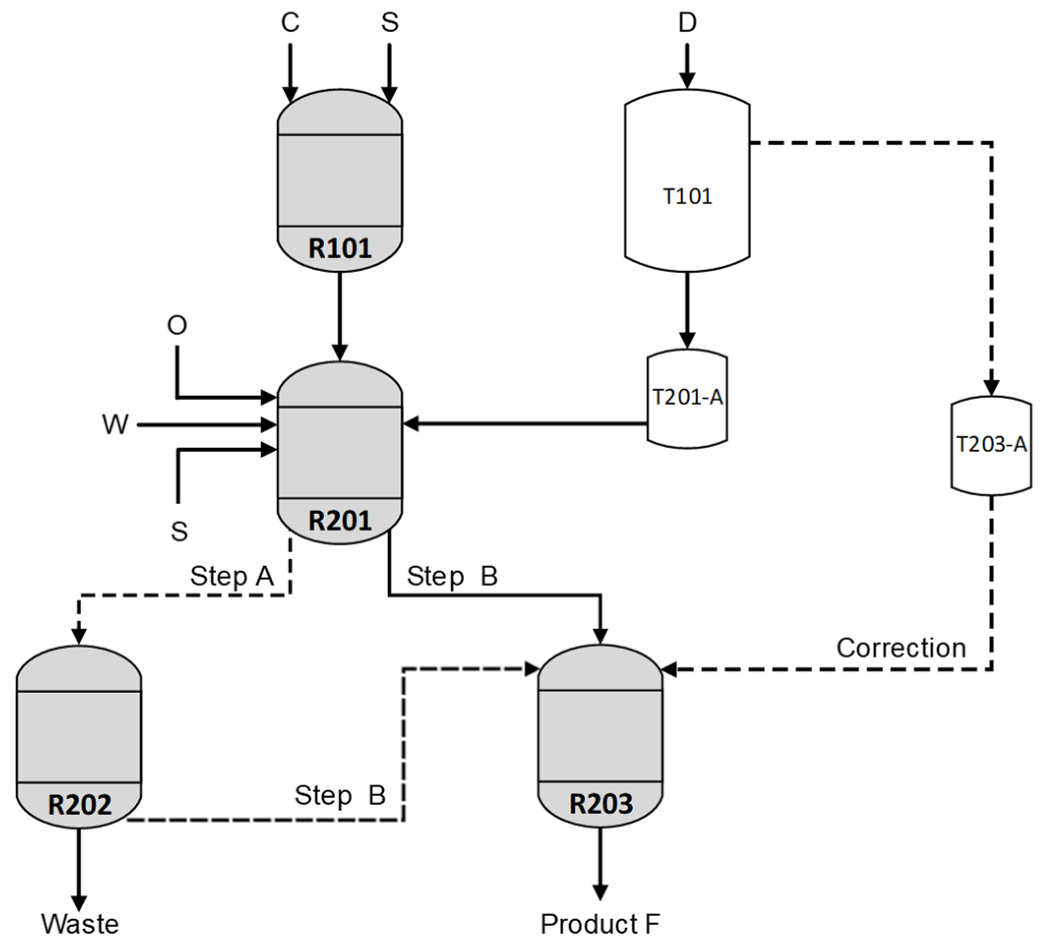
We consider an industrial batch process for the manufacturing of a polymer stability enhancer. The plant layout involves a series-parallel configuration of the processing units, as shown in
Figure 1.
Table 1 summarizes the main characteristics of the units.
The reaction stoichiometry involves two main liquid-phase exothermic reactions:
where C and D are the reactants, E is an intermediate, F is the desired product, and N is a by-product. Some secondary reactions also occur; however, they can be disregarded for the purpose of this study. The product can further react with one of the reactants, according to:
where G and H are subproducts. Some other species are involved in the process: O (which is an additive), S (a solvent), and W (water).
Due to limitations in the size of reactor R201, each batch is carried out through two sequential manufacturing steps. In the first step (step A), a suspension of raw material C in solvent S is obtained in R101; then, the suspension is sent to R201, where reactant D, together with O, S and W, are added, and the synthesis of the desired product F takes place. After an assigned time, the mixture is transferred to R202, whose main task is separating the aqueous solution from the organic phase. However, a minor fraction of the synthesis may also occur in the tank.
In the second manufacturing step (step B), a second charge of reactants with the same amount and composition as in step A is fed to R201 (after suspending it in S using R101), and the reaction is left to occur for the same time as in Step A. Afterwards, the reacted material coming from both steps is transferred to R203, where the synthesis is completed for a given period. At the end of the assigned reaction time, a product sample is collected from R203 and sent to the laboratory for quality assessment.
If the product is found to be out of specification, the batch is denoted as abnormal (or faulty): an additional amount of reactant D (called a “correction”) is fed to R203 according to a semi-empirical rule, and the reaction is left to proceed for an additional assigned time in the attempt to achieve the desired quality. If the amount of required correction is smaller than a given threshold, the batch terminates when the additional time is expired, and no further quality assessment is required. However, if the correction amount is greater than the threshold, at the end of the additional reaction time one more product sample is collected and analyzed: if the product is still found to be out of specification, a further correction is applied and additional reaction time is allowed.
Table 2 reports the fraction of batches that underwent corrections over the three years of operation preceding this study. Over 60% of the batches required at least one correction, meaning that the frequency of corrections was very high. We stress that each correction implies a laboratory analysis, an additional load of reactant, and additional reaction time: all of these actions negatively impact the manufacturing costs and productivity. Additionally, when two corrections are required, R203 becomes the bottleneck for the downstream production line, thus further limiting the plant productivity. Considering that more than 400 batches were typically processed per year, corrections represent a significant issue for the process economics, and therefore there is a very strong incentive to reduce them.
Troubleshooting this process means finding which unit the product quality inconsistency originates from, and the root cause of the abnormality in that unit. The task is not simple because each batch is carried out through two sequential manufacturing steps; each step uses the same reactants and equipment, but the equipment is operated at different times; an additional piece of equipment (R202, conceptually working as a holding tank to decouple the two steps) is used only in one step; finally, no product quality assessment is available until the time at which the batch is expected to terminate.
3. Available Data
A total of
batches spanning a period of 6 consecutive months of operation were extracted from the plant historian. The data were divided into two categories: process data (corresponding to real-time sensor measurements) and quality data (i.e., lab analyses). For each unit, the process data were organized as a three-dimensional array
, where
is the number of measurement sensors available for the unit, and
is the total number of observations per batch. Note that the number of observations changes from batch to batch, not only because a given batch may (or may not) require a correction, but also because the processed material may need to be held in the unit for an extended period because a downstream unit is temporarily not available. Nevertheless, we use a notation where
is the same for all batches; this is a consequence of batch cropping and alignment, a set of pre-processing techniques that will be discussed in
Section 4.
The final product quality is a multivariate property characterized by the concentrations of 5 species (namely D, E, F, G, and other impurities), as obtained from lab measurements. The quality measurements were organized as a matrix including only the concentrations related to the first product sample, because a second sample is not available for all batches.
Overall, the available dataset originally included over 3.5 million data entries. A list of the process variables eventually considered for each unit is reported in the
Appendix A.
4. Mathematical Background
We provide a very short overview of the multivariate statistical techniques used in this study, namely principal component analysis (PCA) and projection on to latent structures (PLS). Details on the techniques and their use for process monitoring can be found elsewhere [
9,
10,
11,
12,
25].
PCA summarizes the information embedded in a dataset ] of samples and variables by projecting the data onto a new coordinate system of orthogonal principal components, which capture the correlation between the variables and identify the direction of maximum variability of the original data.
When correlated variables are present in
, a small number
of principal components is sufficient to describe
, because correlated variables are represented in common variability directions. Hence, by retaining the first
principal components only, the representation of
is:
where
is the scores matrix,
is the loadings matrix,
is the matrix of the residuals.
PLS is a regression technique that relates a set of input variables
to a set of response variables
. It aims at finding a linear transformation of the
data that maximizes the covariance of
and
. Assuming that
latent variables are used, the
and
dataset are decomposed as:
with:
where
and
are the scores matrices, and
and
are the loadings matrices for
and
, respectively;
and
are the residuals matrices for
and
, respectively, which are minimized in a least-squares sense; and
is the
weights matrix that identifies the direction of maximum covariance/correlation among inputs and responses.
For both PCA and PLS, the relevant scores, loadings and weights can be interpreted to analyze the similarity between samples and the correlation among variables within and between datasets. To avoid the scaling effect of different measurement units in the data, both and are pretreated before any transformation is applied. In this study, the columns of and are autoscaled, i.e., the data are mean-centered and scaled to unit variance.
Data coming from systems (e.g., batch processes), whose variables evolve both continuously in time and discontinuously across different runs, can be arranged in a three-way array. The first dimension of the array represents the runs, the second dimension the variables, and the third dimension the time. Multiway multivariate techniques can be exploited to handle this type of data [
12,
26].
5. Proposed Methodology and Results
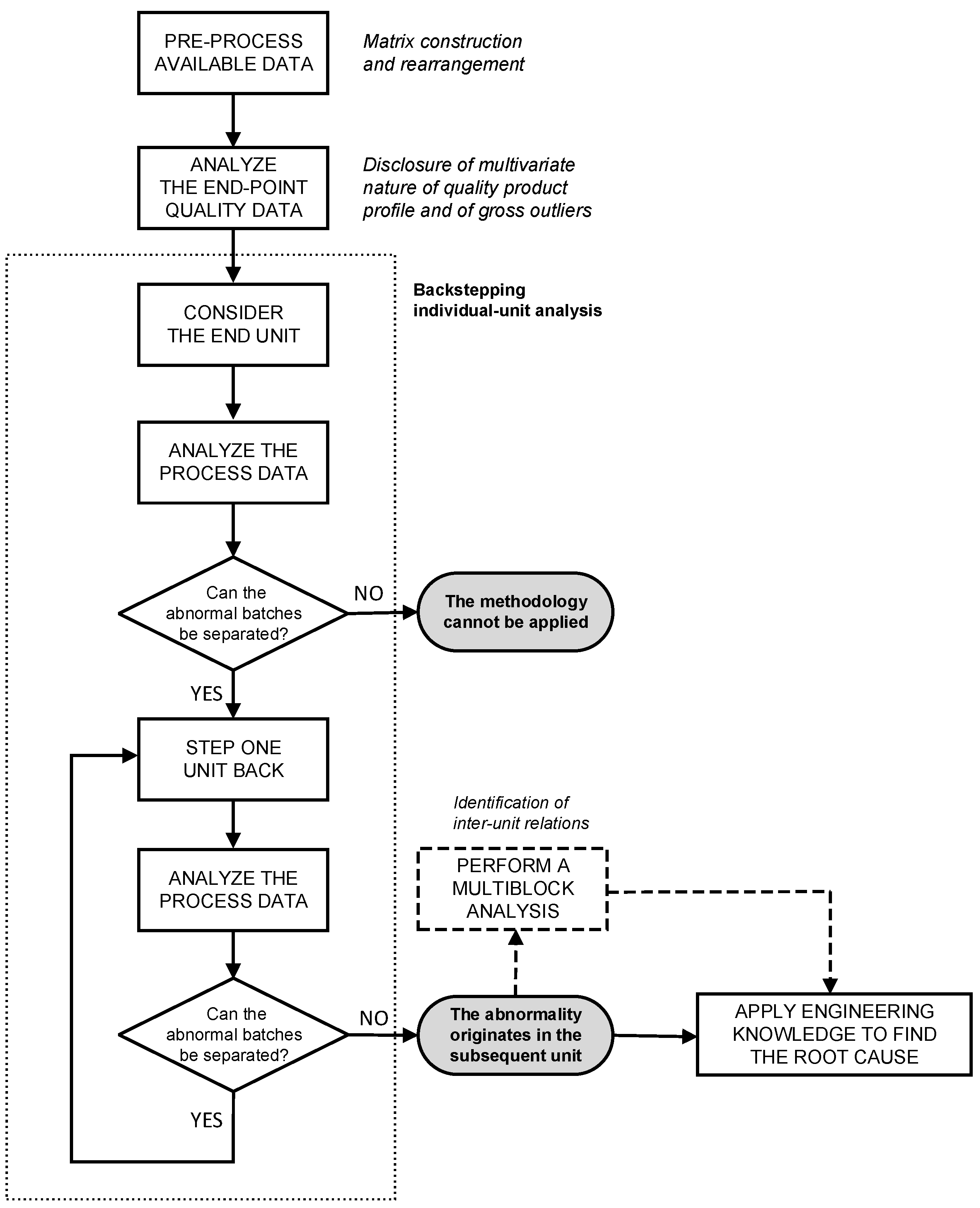
The proposed systematic procedure to assist the troubleshooting of plant-wide batch processes is sketched in
Figure 2 and comprises the following main tasks:
The relations between processing units can be investigated in a separate (optional) multiblock analysis. These tasks are discussed in detail in the following.
5.1. Data Pre-Processing
Pre-processing the available data is required both to arrange them in a form that is appropriate for treatment by PCA and PLS (e.g., mean centering, scaling, imputation of missing data, alignment), and to extract process features whose calculation can help the subsequent analysis.
For the process under investigation, the
dataset did not display any missing data. The fraction of missing data in each of the
matrices was very small. Given that the sampling interval for the plant sensors was much smaller than the characteristic time of the process, the missing data at a given time sample were replaced by simply averaging the data at the previous and subsequent time instants. More sophisticated techniques are available and can work better in other scenarios [
27,
28].
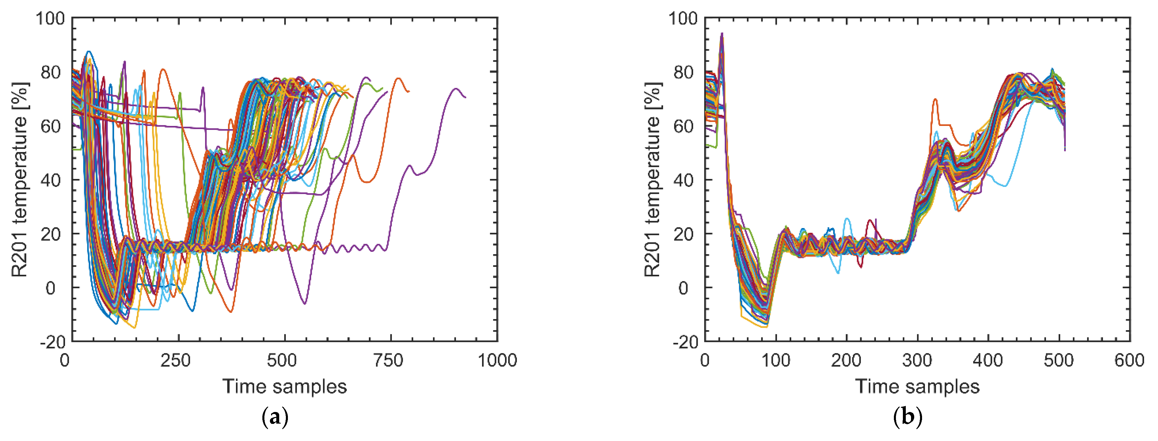
Alignment of the process variable time profiles is required because the batches have different lengths [
29,
30]. Dynamic time warping [
31] proved very effective to this purpose, and allowed batch-wise unfolding [
25] three-way arrays
into two-way matrices
. The trajectory portions corresponding to holding/idle times were removed. Additionally, the trajectories in R203 were cropped to remove the portions extending beyond the first product sample. The effect of a typical alignment task is shown in
Figure 3 for R201 temperature trajectories across several batches.
Feature extraction [
12,
32] uses engineering knowledge to combine the available data in a non-linear fashion, in such a way as to derive new variables that can complement those coming from the plant sensors in order to disclose operation-relevant information that can aid the troubleshooting task. In a way, adding the extracted features to the available dataset represents a way to hybridize the data-driven model with first-principles information, an operation that is known to help fault detection and diagnosis [
33,
34]. One example that proved useful for the process under investigation was including information about the reaction stoichiometry. This was obtained by scaling the reactant loads according to the reaction stoichiometry, and adding the scaled loads to
. Moreover, each reactor was characterized using two additional features: time and heat exchanged. The warped time was added to include information deriving from the trajectory alignment task. In fact, whereas in the original batch trajectories time has a linear evolution across a batch, after alignment it is stretched or compressed. Therefore, the warped time can potentially disclose information about how a batch is evolving with respect to the others [
23]. Information on the rate of heat exchanged in a unit was obtained by either multiplying the utility flow in that unit by the relevant change in temperature, or (in the absence of appropriate sensors) as the cumulative change of the unit temperature.
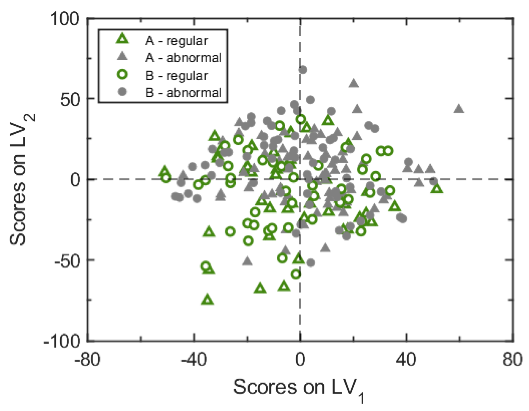
5.2. Analysis of End-Point Quality Data
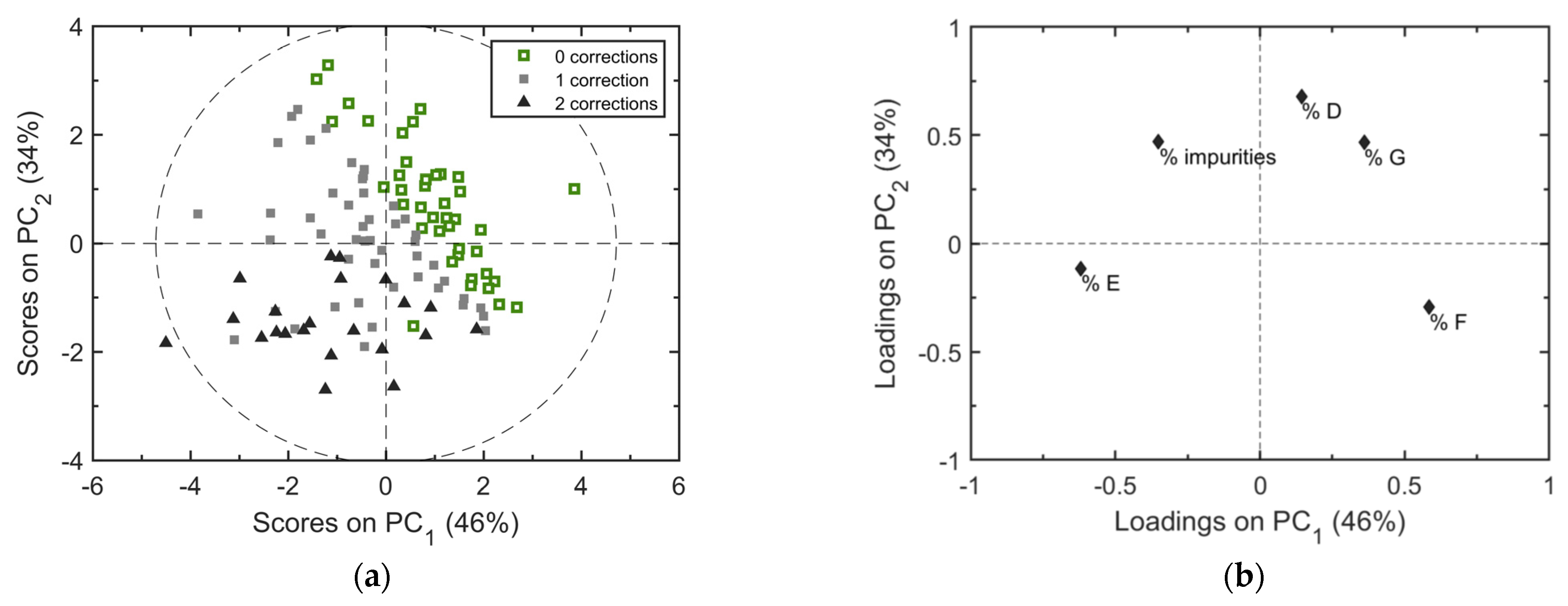
Analysis of the end-point quality data is aimed at revealing graphically the multivariate nature of the product quality profile, and the clustering of regular and faulty batches. PCA can be used to this purpose.
Figure 4 shows the results from a PCA model capturing 80% of the variability of the product quality data through the first two principal components. The scores plot of
Figure 4a reveals that the regular batches can be discriminated from the abnormal ones quite sharply using the product quality data; the quality profile that fingerprints an abnormal batch is visible through the loadings plot of
Figure 4b. The scores plot reveals that the quality data are not sufficient to provide a discrimination between faulty batches undergoing one single correction from those undergoing two corrections. That is an indication that the number of corrections required for a faulty batch is related also to factors that are different from the product quality. One additional piece of information provided by the scores plot of
Figure 4a is that no significant outlier exists in the available dataset (at least from the product quality point of view).
5.3. Backstepping Individual-Unit Analysis of Process Data
The proposed methodology to assist the troubleshooting task is founded on two pillars: (i) an abnormality in a batch leaves a fingerprint not only on the quality data, but also on the process data; (ii) the fingerprint is conserved as the processed material moves across the processing units. If both conditions are met, the propagation of the abnormality through the units can be tracked by carrying out a multivariate analysis of the process data starting from the last unit wherein the abnormality manifests itself, and then moving backwards (according to the process flow diagram and manufacturing recipe) through the preceding units. Stepping back through the units will end-up in a unit U from which no fingerprints of the abnormality can be detected: the unit originating the abnormality will therefore be the one following U. Engineering judgment will finally guide the root-cause analysis.
In the following subsections, this methodology is applied to the reference industrial process. The fingerprint of abnormality in a unit is disclosed by building a PLS discriminant analysis (PLS-DA) model [
35,
36] between the
matrix of that unit and the binary vector
denoting the final batch designation (0 = normal batch; 1 = abnormal batch). No attempt is made to discriminate between batches undergoing one or two corrections.
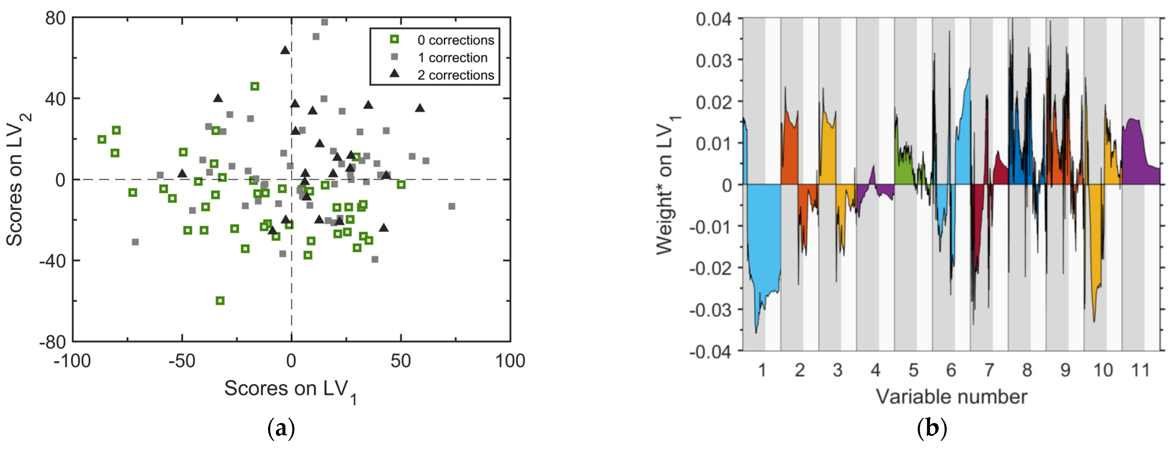
5.3.1. Analysis of R203
A two-component PLS-DA model results in the scores and weights plots of
Figure 5. The scores plots (
Figure 5a) reveals that the separation between regular batches and abnormal ones is not sharp, suggesting that the variability of the final batch designation (normal vs. abnormal) cannot be entirely captured by the process variable trajectories in R203. Stated differently, there are factors that concur in determining the batch designation, but do not leave a fingerprint in the measured process variables. The first quadrant of the scores plane includes a large number of abnormal batches and almost no regular batches, suggesting that (i) there is a relatively large fraction of the abnormal batches that are characterized by a similar pattern of change of the process variable time profiles in R203, and (ii) this pattern is different from that characterizing the regular batches. The subsequent analysis for R203 will focus on these abnormal batches.
The separation of the abnormal batches occurs mainly in the direction of the bisector of the first and third quadrant, which is, therefore, characterized by the weights of the first latent variable. By combined analysis of the scores plot (
Figure 5a) and weights plot for the first latent variable (
Figure 5b), one concludes that the first-quadrant cluster of abnormal batches is characterized by:
greater temperature (variables no. 2 and 3) in the first part of the operation (charge of Step A material;), and smaller temperature in the second part (charge of step B material and reaction). This behavior is highlighted also by the output of the temperature controller (no. 10), and by the integral of the reactor temperature (no. 11);
shorter cycle time (variable no. 1);
greater pressure (variables no. 8 and 9).
The temperature profile patterns deserve attention because the main reactions are exothermic. A higher temperature in the first part of the operation indicates that, for most of the faulty batches, R203 is charged with material (from step A of the process) that is at a temperature greater than the average; for the same batches, the lower temperature during the reaction phase is possibly an indication of lower heat generation from the reaction.
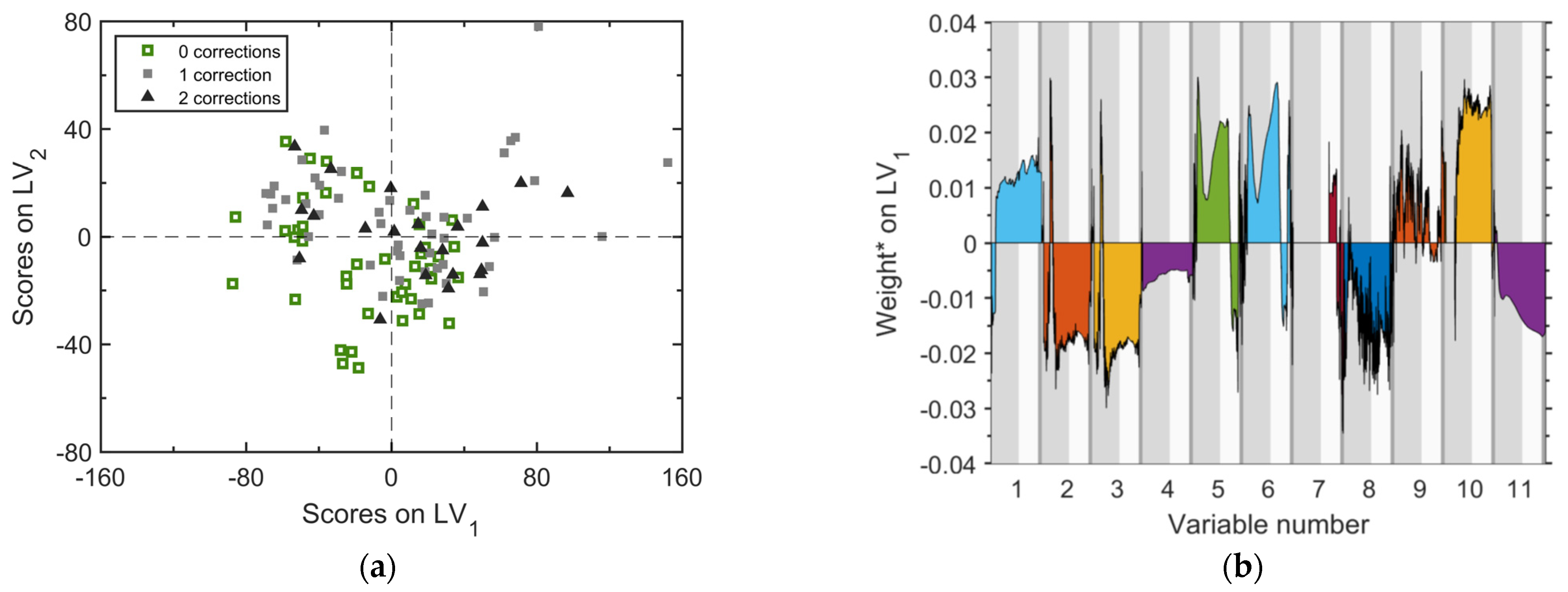
5.3.2. Analysis of R202
According to the proposed methodology, the analysis is carried out for the unit located immediately upstream of R203, namely R202. Recall that this unit is a decanter, which is used also to decouple the two manufacturing steps through which the process is carried out (the material from Step A remains on hold in R202 until the processing of step B material in R201 is completed). The objective of the analysis is understanding whether abnormality fingerprints are embedded also in the trajectories of the process variables of this unit: if that occurs, we conclude that abnormality in a batch arises upstream the end unit.
The results of a PLS-DA model with two principal components are illustrated in
Figure 6; note that the
vector is the same as in the analysis of R203, i.e., it represents the batches that are designated as regular or faulty according to the first product sample that will be collected at a later time from the end unit. The scores plot (
Figure 6a) shows that the separation between regular and abnormal batches is far less sharp than for R203: several regular and faulty batches are clustered around the origin of the scores plane, indicating that (on average) their time evolution is not very different, at least in terms of the measured process variables. Nonetheless, there still exists a fraction of abnormal batches that are separated into the first quadrant with almost no regular batches therein, suggesting that also for this unit the abnormality fingerprints result in patterns of change of the process variables that are distinctive of the abnormal batches only.
From the analysis of the weights reported in
Figure 6b, we can state that the first-quadrant cluster of abnormal batches is characterized by:
longer duration (variable no. 1);
smaller temperature (variables no. 2 and 3), as also confirmed by a greater temperature controller output (variable no. 10);
greater charge, as results from the fact that the weights for the level measurements (variables no. 5 and 6) are greater during the charging stage;
smaller pressure (variable no. 8).
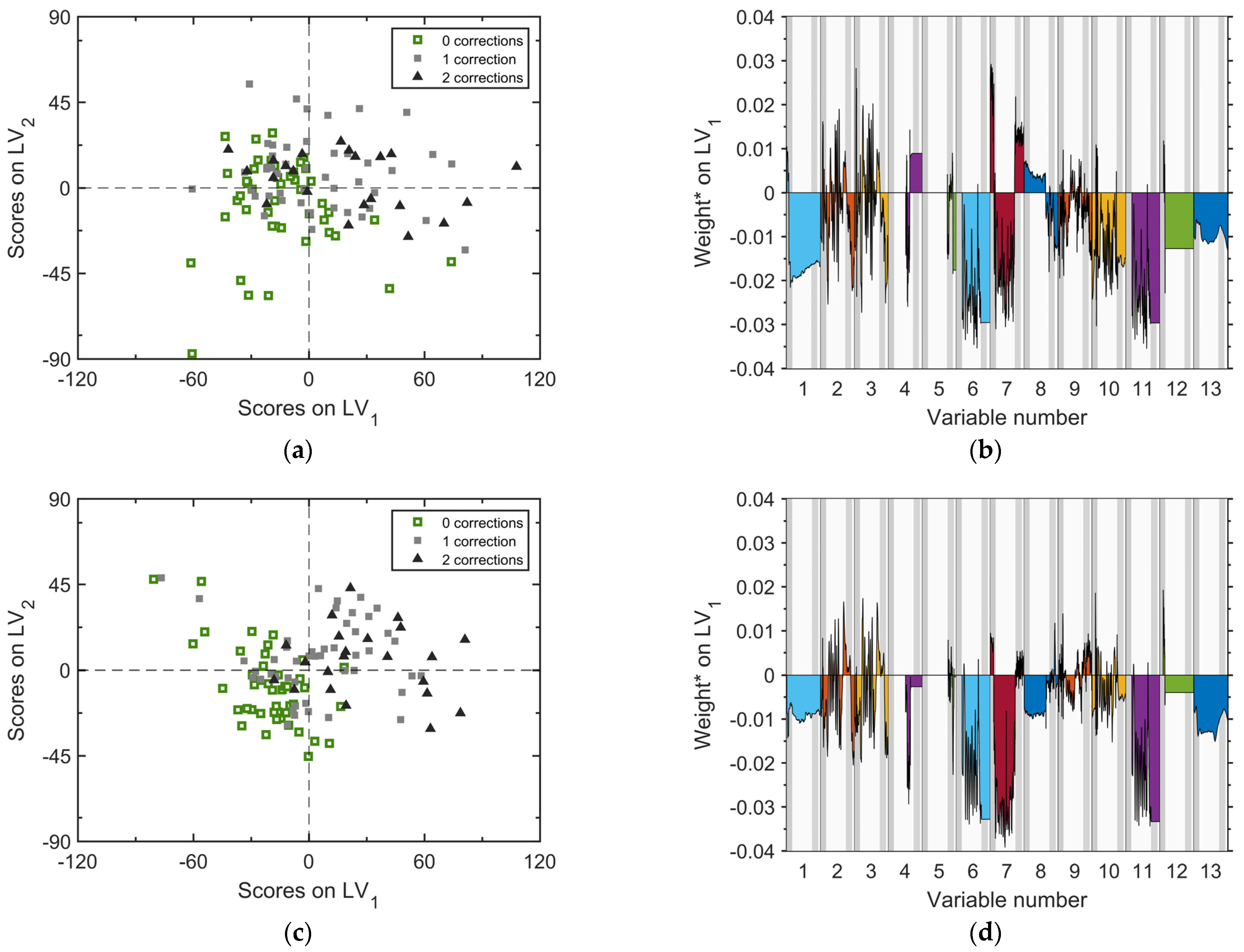
5.3.3. Analysis of R201
As discussed in
Section 2, R201 is a reactor characterized by a much smaller volume than R203. This requires carrying out the same reaction twice in two distinct manufacturing steps (Step A and Step B). In principle, the two steps should be identical. However, to keep track of any possible changes between Step A and Step B (e.g., a change of the equipment’s initial status during Step B due to the reaction carried out in Step A), we analyze the data records belonging to each step separately. The results from the relevant two-component PLS-DA models are illustrated in
Figure 7.
Analysis of the scores plot for Step A (
Figure 7a) and Step B (
Figure 7c) allows us to state that, with respect to abnormality discrimination, R201 does not behave in a strongly different way from R203. In fact, not all the batches, which will be designated as abnormal later in R203, can be early identified as such from the process variables profiles in R201. However, a significant fraction of the abnormal batches (namely, those projecting onto the first quadrant) are characterized by a peculiar pattern of change over time of the process variables while they are being processed in R201, and this pattern is different from that characterizing the regular batches. This means that, for these abnormal batches, the abnormality detected from R203 at the end of the manufacturing process leaves its fingerprint as early as in R201, which in turn makes us conclude the root cause of the abnormality does not lie in either R203 or R202. That is useful information for process troubleshooting, because it restricts the domain of units that need to be investigated to find the root cause of the fault. Interestingly,
Figure 7c shows that the model built on the data related to Step B has a slightly greater discrimination ability than the model built on Step A data.
The weights plots of
Figure 7b (Step A) and
Figure 7d (Step B) suggest the following considerations with respect to the abnormal batches clustered in the first quadrant for each step:
they are shorter (variable no. 1);
they are run at slightly smaller temperature: even if the weights of the reactor temperature profiles (variables no. 2 and 3) are particularly noisy and, therefore, hard to analyze, the integral of temperature (no. 13) provides a clear view of the overall effect of temperature;
they are characterized by smaller loads of reactant D, as highlighted by the totalized profiles of three flowrate sensors (variables no. 6, 11, 12), and by the level sensor (no. 7).
With reference to the latter point, note that the weights on variables no. 6, 7 and 11 are much stronger that the other weights, suggesting that the effect of the charge of reactant D in the cluster formation is dominant.
5.3.4. Analysis of R101
The analysis proceeds by stepping one more unit back. Since no reaction takes places in R101, the charges related to Step A and Step B are analyzed jointly in a single PLS-DA model, whose scores plot for the first two components are shown in
Figure 8.
We notice that the charges later requiring one or two corrections in R203 cannot be distinguished from those that will be labeled as regular. We conclude that the fingerprints of abnormality are not visible in R101, i.e., that unit U is R101. Therefore, the unit originating the observed product quality inconsistency is the next one in the process flow diagram (namely, R201).
5.4. Multiblock Analysis
Having identified the unit wherefrom the fault originates, an overall global multiblock analysis [
37,
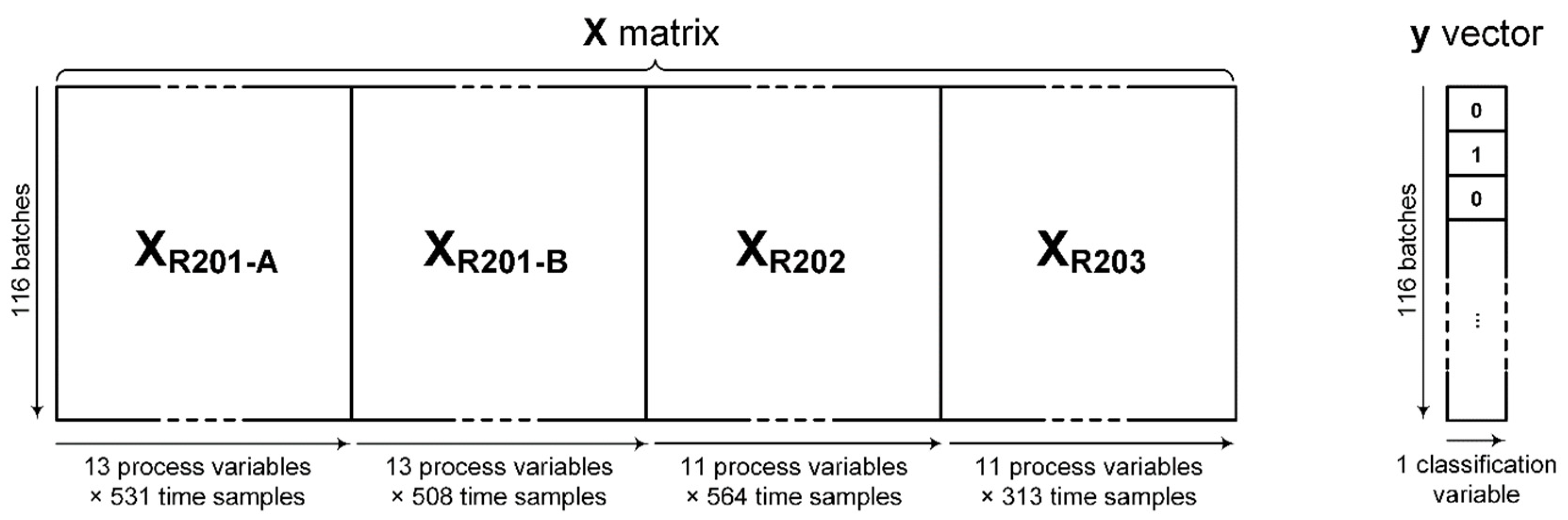
38] may be carried out across all units where the fault leaves its fingerprint. This can disclose relations between the units that are not visible when the units are analyzed one at a time, and highlight the relative importance across the units of the process variables that most contribute to differentiate regular batches from faulty ones. The
matrix for the PLS-DA multiblock model is built by placing the
matrices of the individual units side by side, as illustrated in
Figure 9; the classification vector
is the same as in the individual-unit analysis.
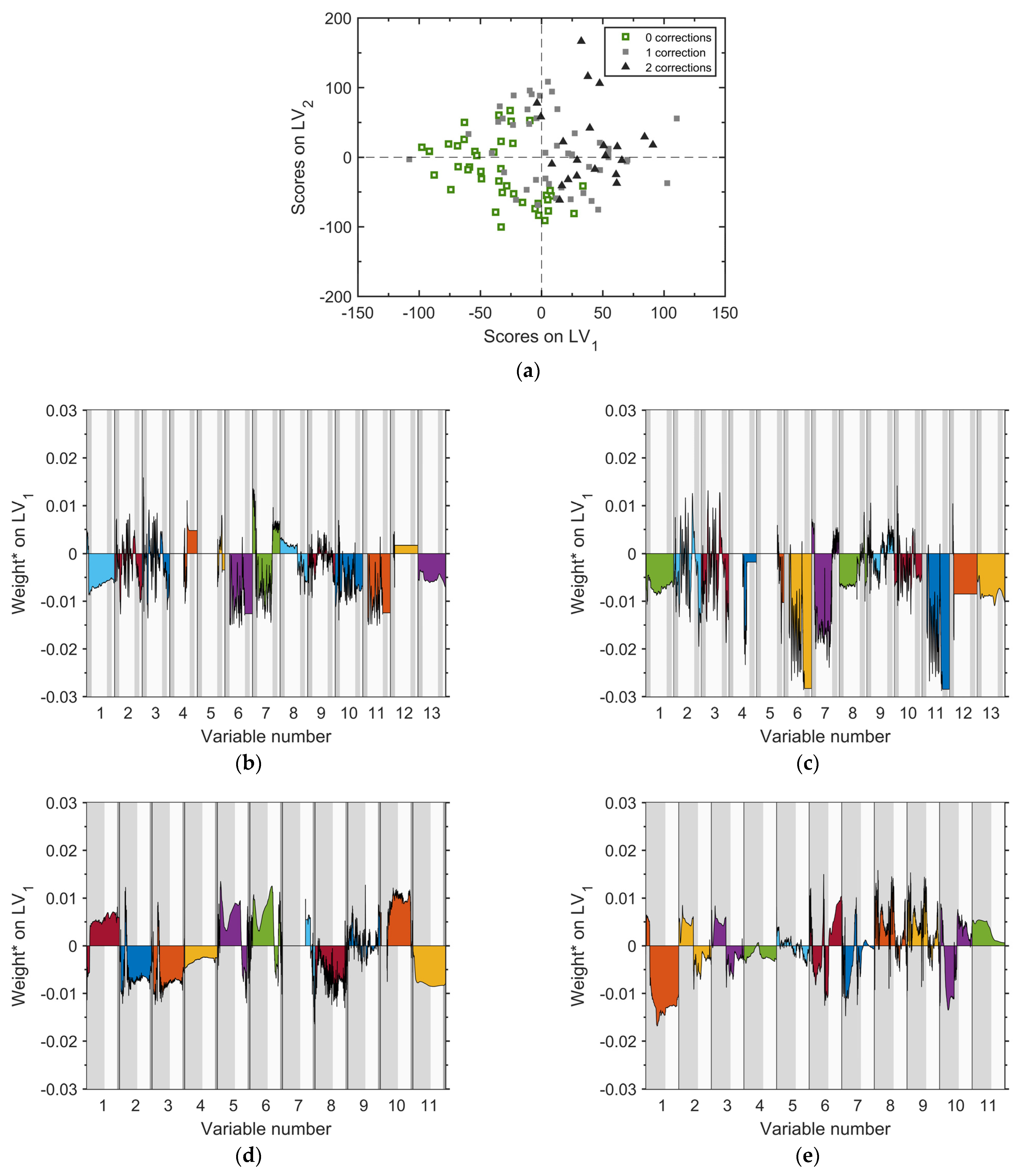
The scores plot for the first two components (
Figure 10a) is similar to those obtained for the individual units; the separation between regular and abnormal batches is actually even sharper, with most of the abnormal batches located in the first quadrant. The weights plots of
Figure 10b–e provide insights about the variables that most contribute to the separation. The dominant effect is provided by variables no. 6, 7 and 11 of
Figure 10c, namely by the insufficient load of reactant D to R201-Step B. This result confirms the previous findings, and suggests a need to complete the troubleshooting task by using engineering judgment to find the root cause that determines an abnormal load of reactant D in R201.
5.5. Root-Cause Analysis
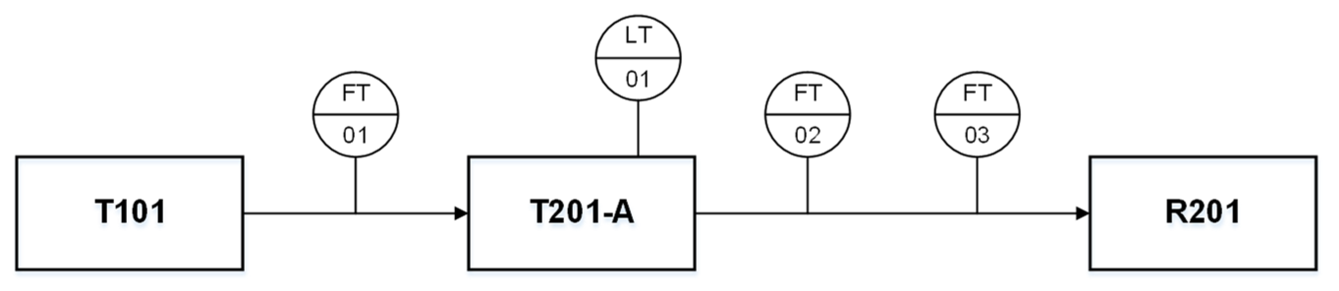
Figure 11 is a sketch of the process of reactant D feeding into reactor R201. First, an amount
of D (equal to the one required by the reaction stoichiometry) is loaded into a buffer tank (T201-A). Then, when R201 is ready to receive the reactant, T201-A is fully discharged into R201. A level sensor is available in T201-A, and three mass flow meters are available in the feed lines; each flow meter also works as a mass totalizer. A distributed control system handles the feeding sequence: FT-01 is responsible for charging reactant D into T-201-A; LT-01 takes care of the discharge of D into R201; FT-02 and FT-03 are (respectively) a safety sensor and a sensor ensuring that a minimum amount of reactant is always fed to R201. Insufficient load of reactant D into R201 may result from malfunctioning of FT-01 and/or LT-04 (the other equipment involved in the reactant transfer, e.g., pumps and valves, are known to work appropriately). We challenge the assumption that FT-01 does not work properly.
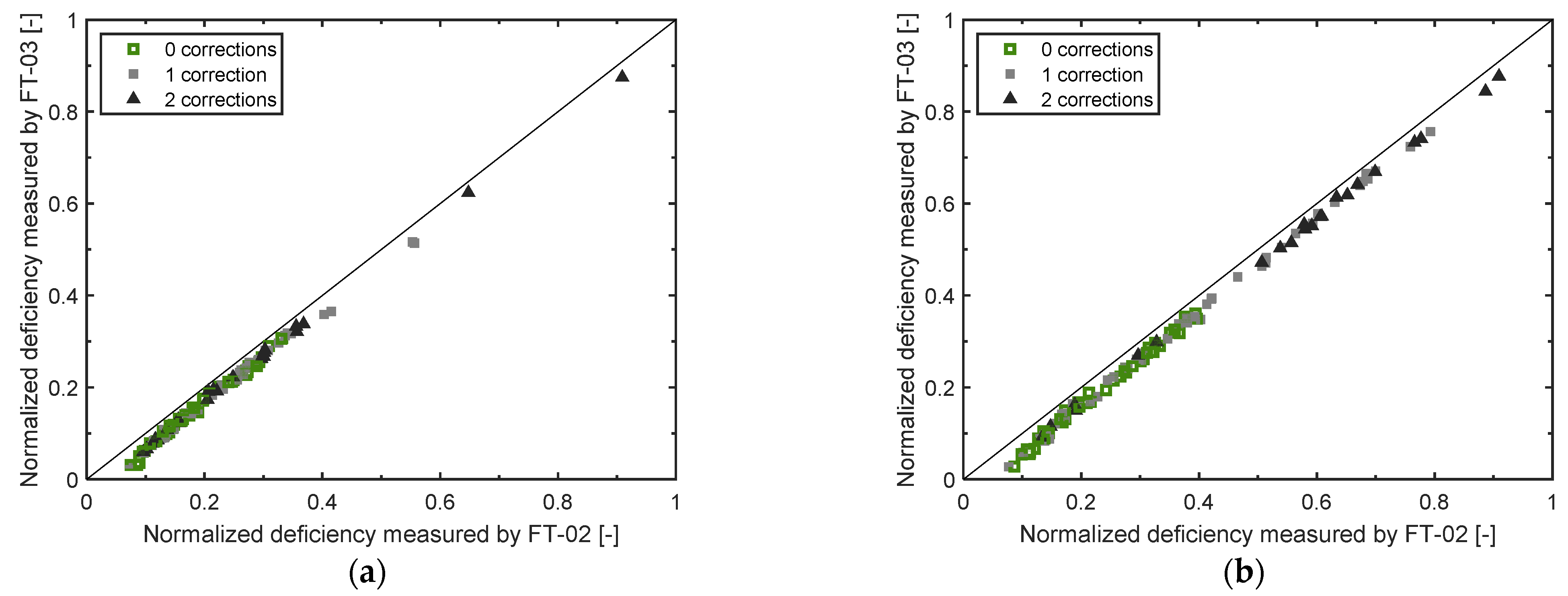
For each manufacturing step, we build a parity plot where the deficiencies of reactant D as measured by the two flow sensors downstream T201-A are contrasted (
Figure 12). Namely, the variables in each parity plot are the difference between
and the totalized mass transferred to R201 as read by FT-02 (
x-axis) and by FT-03 (
y-axis).
Since the measured deficiencies in reactant D align well along the diagonal both for Step A (
Figure 12a) and for Step B (
Figure 12b), we conclude that either FT-02 and FT-03 are both faulty and affected by the same fault (a very unlikely situation), or the faulty sensor is FT-01. Furthermore, analysis of
Figure 12b suggests that a very large fraction of the batches later requiring corrections in R203 are characterized by a deficiency in the amount of D loaded into R201 during Step B.
A further investigation revealed that the totalized mass signals from FT-02 and FT-03 are strongly correlated not only to each other, but also to the level signal from LT-01. On the other hand, the totalized mass read from FT-01 is neither correlated to the T-201A level signal, nor to any of the other two totalized mass signals.
This evidence makes the troubleshooting task come to an end: sensor FT-01 is faulty, and the fault manifests itself mainly during Step B of the manufacturing process. When it does, less reactant D than needed is loaded into R201, and this ends up in a batch needing at least one correction after the processing in R203. Nonetheless, there still remain other causes, which determine abnormality in a batch, that cannot be captured by the available field sensors. This occurs for the abnormal batches (less than one third of the total number of abnormal batches) with a deficiency of reactant D smaller than 0.4 in
Figure 12b.
5.6. Field Testing
Following the indications obtained by application of the proposed methodology, the faulty sensor was substituted. The impact of the troubleshooting was assessed after one year of plant operation with the new sensor. The results are summarized in
Table 3.
A comparison with
Table 1 reveals that the fraction of batches requiring corrections was halved, with almost no batches requiring two corrections. This ended up in a significant reduction of the overall cycle time, and a related 6% increase of productivity.
6. Conclusions
We have presented a systematic methodology to troubleshoot plant-wide batch processes characterized by abnormal variability in the end-product quality. It couples the use of multivariate statistical methods with engineering judgment to extract operation-relevant information from a topologically ordered set of processing units that operate along different time windows and with different charges of material. Its main value is that it is based on a structured approach enabling the user to first identify the unit originating the fault, and then look for the root causes of the fault within that unit.
The methodology is characterized by a backstepping multivariate analysis of the processing units. The end unit (i.e., the one where the product is eventually collected from) is the first to be analyzed, using the signals from the field sensors in order to discriminate the abnormal batches from the regular ones. Then, the analysis is repeated by stepping one unit back according to the process flow diagram and the manufacturing recipe. The backstepping ends when a unit is found where the field sensors cannot capture clear fingerprints of batch abnormality any more. Once the unit from which the fault likely originates has been found, engineering judgment can guide the fault isolation step.
We have proved the effectiveness of the proposed methodology by troubleshooting a plant-wide batch process that manufactures a polymer stability enhancer. The complexity of the process lies in the fact that some of the units are used at different times with different charges of material within the same production cycle, and no product quality measurements are available until the end of the cycle. The product quality inconsistency was shown to originate from a faulty sensor located at the very beginning of the process flow diagram. Correction of the fault allowed for a significant increase of the productivity.
Author Contributions
Conceptualization, P.F., F.B. and M.B.; methodology, P.F., F.B. and M.B.; software, F.Z.; validation, F.Z., M.C., P.F., F.B. and M.B.; formal analysis, P.F., F.B. and M.B.; investigation, F.Z., M.C., P.F., F.B. and M.B.; data curation, F.Z.; writing—original draft preparation, F.Z.; writing—review and editing, M.B.; visualization, F.Z.; supervision M.B.; funding acquisition, M.B. All authors have read and agreed to the published version of the manuscript.
Funding
This research was funded by the University of Padova under project BIRD194889-SID 2019 “Augmenting data-driven models with knowledge-driven information to enhance process monitoring in the Industry 4.0 era (AUGH)”.
Institutional Review Board Statement
Not applicable.
Informed Consent Statement
Not applicable.
Data Availability Statement
Not applicable.
Conflicts of Interest
The authors declare no conflict of interest. F.Z. and M.C. are employees of BASF Italia.
Appendix A
List of the process variables eventually analyzed for each unit.
Table A1.
List of the process variables analyzed for unit R101.
Table A1.
List of the process variables analyzed for unit R101.
| ID | Description |
|---|
| 1 | Warped time |
| 2 | Measured weight [kg] |
| 3 | Internal temperature (sensor 1) [°C] |
| 4 | Internal temperature (sensor 2) [°C] |
| 5 | Totalized flowrate of C [kg] |
| 6 | Totalized flowrate of S (inlet) [kg] |
| 7 | Totalized flowrate of S (tank) [kg] |
| 8 | Measured level [L] |
| 9 | Calculated level [L] |
| 10 | Inlet density of C [kg/L] |
| 11 | Inlet pressure of C [bar] |
| 12 | Exchanged heat [W] |
| 13 | Integral of the internal temperature [°Cs] |
Table A2.
List of the process variables analyzed for unit R201.
Table A2.
List of the process variables analyzed for unit R201.
| ID | Description |
|---|
| 1 | Warped time |
| 2 | Internal temperature (sensor 1) [°C] |
| 3 | Internal temperature (sensor 2) [°C] |
| 4 | Mass flowrate of W [kg/h] |
| 5 | Totalized flowrate of O [kg] |
| 6 | Totalized flowrate of D (sensor 1) [kg] |
| 7 | Measured level (R201) [L] |
| 8 | Measured level (additive O tank) [L] |
| 9 | Internal pressure (R201) [mbar] |
| 10 | Internal pressure (T201-A) [mbar] |
| 11 | Totalized mass of D (sensor 2) [kg] |
| 12 | Totalized mass of D (sensor 3) [kg] |
| 13 | Integral of the internal temperature [°Cs] |
Table A3.
List of the process variables analyzed for unit R202.
Table A3.
List of the process variables analyzed for unit R202.
| ID | Description |
|---|
| 1 | Warped time |
| 2 | Internal temperature (sensor 1) [°C] |
| 3 | Internal temperature (sensor 2) [°C] |
| 4 | Condensate temperature [°C] |
| 5 | Measured level [L] |
| 6 | Calculated level [L] |
| 7 | Outlet density [kg/L] |
| 8 | Internal pressure [bar] |
| 9 | Cooling fluid pressure [bar] |
| 10 | Controller output (internal temperature) [%] |
| 11 | Integral of the internal temperature [°Cs] |
Table A4.
List of the process variables analyzed for unit R203.
Table A4.
List of the process variables analyzed for unit R203.
| ID | Description |
|---|
| 1 | Warped time |
| 2 | Internal temperature (sensor 1) [°C] |
| 3 | Internal temperature (sensor 2) [°C] |
| 4 | Condensate temperature [°C] |
| 5 | Mass flowrate of W (heat exchanger) [kg/h] |
| 6 | Measured level [L] |
| 7 | Calculated level [L] |
| 8 | Internal pressure (sensor 1) [mbarg] |
| 9 | Internal pressure (sensor 2) [mbar] |
| 10 | Controller output (internal temperature) [%] |
| 11 | Integral of the internal temperature [°Cs] |
References
- Korovessi, E.; Linninger, A.A. (Eds.) Batch Processes; Taylor & Francis: Boca Raton, FL, USA, 2005. [Google Scholar]
- Diwekar, U. Batch Processes—Modeling and Design; CRC Press: Boca Raton, FL, USA, 2014. [Google Scholar]
- Sharratt, P.N. (Ed.) Handbook of Batch Process Design; Chapman & Hall: London, UK, 1997. [Google Scholar]
- Woods, D.R. Successful Trouble Shooting for Process Engineers—A Complete Course in Case Studies; Wiley-VCH Verlag GmbH & Co.: Weinheim, Germany, 2006. [Google Scholar]
- Udugama, I.A.; Gargalo, C.L.; Yamashita, Y.; Taube, M.A.; Palazoglu, A.; Young, B.R.; Gernaey, K.V.; Kulahci, M.; Bayer, C. The role of big data in industrial (bio)chemical process operations. Ind. Eng. Chem. Res. 2020, 59, 15283–15297. [Google Scholar] [CrossRef]
- Qin, S.J.; Chiang, L.H. Advances and opportunities in machine learning for process data analytics. Comput. Chem. Eng. 2019, 126, 465–473. [Google Scholar] [CrossRef]
- Piccione, P.M. Realistic interplays between data science and chemical engineering in the first quarter of the 21stcentury: Facts and a vision. Chem. Eng. Res. Des. 2019, 147, 668–675. [Google Scholar] [CrossRef]
- Reis, M.S.; Gins, G. Industrial Process Monitoring in the Big Data/Industry 4.0 Era: From Detection, to Diagnosis, to Prognosis. Processes 2017, 5, 35. [Google Scholar] [CrossRef] [Green Version]
- Geladi, P.; Kowalski, B.R. Partial Least-Squares Regression: A Tutorial. Anal. Chim. Acta 1986, 185, 1–17. [Google Scholar] [CrossRef]
- Wold, S.M.; Martens, H.; Wold, H. The multivariate calibration problem in chemistry solved by the PLS method. Lect. Notes Math. 1983, 973, 286–293. [Google Scholar]
- Kourti, T.; MacGregor, J.F. Process analysis, monitoring and diagnosis, using multivariate projection methods. Chemom. Intell. Lab. Syst. 1995, 28, 3–21. [Google Scholar] [CrossRef]
- Nomikos, P.; MacGregor, J.F. Monitoring batch processes using multiway principal component analysis. AIChE J. 1994, 40, 1361–1375. [Google Scholar] [CrossRef]
- Kumar, A.; Bhattacharya, A.; Flores-Cerrillo, J. Data-driven process monitoring and fault analysis of reformer units in hydrogen plants: Industrial application and perspectives. Comput. Chem. Eng. 2020, 136, 106756. [Google Scholar] [CrossRef]
- Jiang, Q.; Li, J.; Yan, X. Performance-driven optimal design of distributed monitoring for large-scale nonlinear processes. Chemom. Intell. Lab. Syst. 2016, 155, 151–159. [Google Scholar] [CrossRef]
- Kano, M.; Nakagawa, Y. Data-based process monitoring, process control, and quality improvement: Recent developments and applications in steel industry. Comput. Chem. Eng. 2008, 32, 12–24. [Google Scholar] [CrossRef] [Green Version]
- MacGregor, J.F.; Jaeckle, C.; Kiparissides, C.; Koutoudi, M. Process monitoring and diagnosis by multiblock PLS methods. AIChE J. 1994, 40, 826–838. [Google Scholar] [CrossRef]
- Liu, J.; Chen, J.; Wang, D. Wavelet functional principal component analysis for batch process monitoring. Chemom. Intell. Lab. Syst. 2020, 196, 103897. [Google Scholar] [CrossRef]
- Wu, O.; Bouaswaig, A.; Imsland, L.; Schneider, S.M.; Roth, M.; Leira, F.M. Campaign-based modeling for degradation evolution in batch processes using a multiway partial least squares approach. Comput. Chem. Eng. 2019, 128, 117–127. [Google Scholar] [CrossRef]
- Onel, M.; Kieslich, C.A.; Guzman, Y.A.; Floudas, C.A.; Pistikopoulos, E.N. Big data approach to batch process monitoring. Simultaneous fault detection and diagnosis using nonlinear support vector machine-based feature selection. Comput. Chem. Eng. 2018, 115, 46–63. [Google Scholar] [CrossRef] [PubMed]
- Zhao, L.; Zhao, C.; Gao, F. Inner-phase analysis based statistical modeling and online monitoring for uneven multiphase batch Processes. Ind. Eng. Chem. Res. 2013, 52, 4586–4596. [Google Scholar] [CrossRef]
- Wong, C.W.L.; Escott, R.; Martin, E.; Morris, J. The integration of spectroscopic and process data for enhanced process performance monitoring. Canad. J. Chem. Eng. 2008, 86, 905–923. [Google Scholar] [CrossRef]
- Camacho, J.; Picó, J. Online monitoring of batch processes using multi-phase principal component analysis. J. Process Control 2006, 16, 1021–1035. [Google Scholar] [CrossRef]
- García-Muñoz, S.; Kourti, T.; MacGregor, J.F.; Mateos, A.G.; Murphy, G. Troubleshooting of an Industrial Batch Process Using Multivariate Methods. Ind. Eng. Chem. Res. 2003, 42, 3592–3601. [Google Scholar] [CrossRef]
- Kourti, T. Multivariate dynamic data modeling for analysis and statistical process control of batch processes, start-ups and grade transitions. J. Chemom. 2003, 17, 93–109. [Google Scholar] [CrossRef]
- Wise, B.M.; Gallagher, N.B. The process chemometrics approach to process monitoring and fault detection. J. Process Control 1996, 6, 329–348. [Google Scholar] [CrossRef]
- Camacho, J.; Picó, J.; Ferrer, A. Bilinear modelling of batch processes. Part I: Theoretical discussion. J. Chemom. 2008, 22, 299–308. [Google Scholar]
- Folch-Fortuny, A.; Arteaga, F.; Ferrer, A. PCA model building with missing data: New proposals and a comparative study. Chemom. Intell. Lab. Syst. 2015, 146, 77–88. [Google Scholar] [CrossRef]
- Imtiaz, S.A.; Shah, S.L. Treatment of missing values in process data analysis. Canad. J. Chem. Eng. 2008, 86, 838–858. [Google Scholar] [CrossRef]
- Westerhuis, J.A.; Kourti, T.; MacGregor, J.F. Comparing alternative approaches for multivariate statistical analysis of batch process data. J. Chemom. 1999, 13, 397–413. [Google Scholar] [CrossRef]
- Kourti, T.; Lee, J.; MacGregor, J.F. Experiences with industrial applications of projection methods for multivariate statistical process control. Computers Chem. Eng. 1996, 20, 745–750. [Google Scholar] [CrossRef]
- Kassidas, A.; MacGregor, J.F.; Taylor, P.A. Synchronization of batch trajectories using dynamic time warping. AIChE J. 1998, 44, 864–875. [Google Scholar] [CrossRef]
- Yoon, S.; MacGregor, J.F. Incorporation of external information into multivariate PCA/PLS models. IFAC Proc. Vol. 2001, 34, 105–110. [Google Scholar] [CrossRef]
- Destro, F.; Facco, P.; García-Muñoz, S.; Bezzo, F.; Barolo, M. A hybrid framework for process monitoring: Enhancing data-driven methodologies with state and parameter estimation. J. Process Control 2020, 92, 333–351. [Google Scholar] [CrossRef]
- Tomba, E.; Facco, P.; Bezzo, F.; García-Muñoz, S.; Barolo, M. Combining fundamental knowledge and latent variable techniques to transfer process monitoring models between plants. Chemom. Intell. Lab. Syst. 2012, 116, 67–77. [Google Scholar] [CrossRef]
- Brereton, R.G.; Loyd, G.R. Partial least squares discriminant analysis: Taking the magic away. J. Chemom. 2014, 28, 213–225. [Google Scholar] [CrossRef]
- Barker, M.; Rayens, W. Partial least squares for discrimination. J. Chemom. 2003, 17, 166–173. [Google Scholar] [CrossRef]
- Perk, S.; Çinar, A. Batch process monitoring using multiblock multiway principal component analysis. IFAC Proc. Vol. 2009, 39, 209–214. [Google Scholar] [CrossRef] [Green Version]
- Westerhuis, J.A.; Kourti, T.; MacGregor, J.F. Analysis of multiblock and hierarchical PCA and PLS models. J. Chemom. 1998, 12, 301–321. [Google Scholar] [CrossRef]
| Publisher’s Note: MDPI stays neutral with regard to jurisdictional claims in published maps and institutional affiliations. |
© 2021 by the authors. Licensee MDPI, Basel, Switzerland. This article is an open access article distributed under the terms and conditions of the Creative Commons Attribution (CC BY) license (https://creativecommons.org/licenses/by/4.0/).


 and
and 


