Prediction of Sugar Content in Port Wine Vintage Grapes Using Machine Learning and Hyperspectral Imaging

Abstract

The high quality of Port wine is the result of a sequence of winemaking operations, such as harvesting, maceration, fermentation, extraction and aging. These stages require proper monitoring and control, in order to consistently achieve the desired wine properties. The present work focuses on the harvesting stage, where the sugar content of grapes plays a key role as one of the critical maturity parameters. Our approach makes use of hyperspectral imaging technology to rapidly extract information from wine grape berries; the collected spectra are fed to machine learning algorithms that produce estimates of the sugar level. A consistent predictive capability is important for establishing the harvest date, as well as to select the best grapes to produce specific high-quality wines. We compared four different machine learning methods (including deep learning), assessing their generalization capacity for different vintages and varieties not included in the training process. Ridge regression, partial least squares, neural networks and convolutional neural networks were the methods considered to conduct this comparison. The results show that the estimated models can successfully predict the sugar content from hyperspectral data, with the convolutional neural network outperforming the other methods.

1. Introduction

Produced from grapes of excellent quality that grow in the Douro region, Port wine is known for its renowned quality, being one of the most famous Portuguese fortified wines worldwide. In this work, we consider one well-known representative of Port wines, the Dow’s Port wine (from Symington Family Estates, the industrial partner collaborating with the present research project). This wine is mainly produced from grape varieties harvested in the vineyard of Quinta do Bomfim, often consisting of Tawny Ports, twenty, thirty and forty-year-old wine, aged in oak cask. It is important to keep in mind, however, that the high quality of these wines starts at the vineyards, where it is crucial to monitor the components and properties of the grapes that will be used as raw material for the winemaking process. Such careful control is instrumental to determine the harvesting date and to select the grapes at the optimal maturity stage according to the desired traits. This work is devoted to the development and test of a rapid and informative approach that supports wine makers in this decisive phase of the process. However, all the remaining stages, namely maceration, fermentation, extraction and aging, also need to be properly controlled to accomplish the desired wine properties. Given the importance of the harvesting stage, considerable efforts have been traditionally made by producers and researchers for controlling and monitoring the quality of the grapes, through the evaluation of relevant enological parameters over time with the aid of conventional physical and chemical methods performed off-line. Nevertheless, these standard evaluation protocols present the following disadvantages: they are time-consuming, expensive, invasive, generate chemical waste and are limited to a few samples [1].

With the advancement of technology and the need for rapid, less expensive and non-destructive assessment of wine grape ripeness, optical sensing technologies, including visible and near infrared spectroscopy [2,3], fluorescence-based sensors [4,5], hyperspectral imaging [1,6], have been demonstrated to be useful in assessing grape maturity. Among them, hyperspectral imaging has emerged as an attractive and viable technology [7,8,9,10] to estimate relevant enological parameters in grape berries, showing high potential to support critical decision-making during harvesting, since it combines spectroscopy with digital imaging techniques [11] that allows the collection of process information from across the electromagnetic spectrum in few seconds. In reflectance mode, hyperspectral imaging collects information about how grapes reflect and absorb light as a function of their wavelength [12,13], allowing the analysis of large number of samples and opens the possibility to analyze the grape maturation locally in the vineyards, a highly regarded feature for the wine industry. Besides the reflectance mode, transmittance has also been used in spectroscopy to determine the enological parameters in grapes, although less frequently [14,15,16]. These two spectroscopic modes (reflectance and transmittance) mainly differ in the position of the sample with respect to the light source and detector. In the reflectance mode, the light source and the detector (hyperspectral camera) are placed above the sample while in the transmittance mode, the light source and the detector are positioned on opposite sides of the sample and the light must pass through the sample. The transmittance mode has the disadvantage of requiring a closer proximity to the sample because the intensity of the light is significantly attenuated when passing though the samples. For this reason, the reflectance mode is usually preferred [1,17].

Given the large amount of complex data produced by hyperspectral cameras, data analysis tools are required to properly convert the spectral data into the desired enological information. In this context, the use of advanced machine learning methods, in combination with hyperspectral technology in reflectance mode, has been proven to be a valid line of research to properly deal with the complexity of data, and to extract the relevant information for the prediction of enological parameters in grapes berries [1,2,3,18,19,20,21,22,23,24,25,26,27,28,29]. One of the main advantages of using machine learning methods relies on their ability to generalize, i.e., to estimate the enological parameters for future samples, once a proper calibration of the system is done, using training samples and the corresponding enological parameters. Nevertheless, monitoring the level of maturation is a complex problem due to the large variability of grape composition, grape variety and terroirs over time. Thus, assessing the generalization ability of a model for different vintages and varieties is an important task, in order to assess the robustness of the final methodology. Despite the existence of numerous works published in the literature for grape ripeness assessment, most of them address the case of samples from no more than one or two harvested years. In fact, the generalization assessment of machine learning models is almost absent from the technical literature, with the exception of a few works where models were trained with grapes from one vintage/variety and tested with grapes from another vintage/variety [2,18,22,27,29].

The present work reports the development of four different machine learning (ML) methods, including a deep learning approach, towards the assessment of grape ripeness and in particular the sugar content. The sugar content is an essential maturity index in the wine industry, and is directly related with the alcoholic strength of the wine. The ML methods considered are ridge regression (RR); partial least squares regression (PLSR); artificial neural networks (NN); and one-dimensional convolutional neural networks (1D CNN). These methods are developed and compared using an extensive dataset composed of several vintages of one variety for training, and different vintages and varieties used for testing and not employed during training. This rich dataset also incorporates the effects of natural variability such as that originated from differences between grape varieties, climate factors, sun exposition, varying water availability, heterogeneous soil quality and different altitudes, etc., which is a fundamental aspect for assessing the performance in real world conditions. Indeed, it is relevant to carry out this comparison among such different machine learning methods since the assumptions of each proposed method is different, and it is impossible to know in advance which method is most suitable for the proposed problem. The choice of using partial least squares [3,18,19,21,23,25,26,27,28] and neural networks [1,18,29,30] methods in the current work was based on the fact that these are the most commonly applied approaches in the scientific literature for predicting enological parameters of grape berries from spectroscopic data. On the other hand, ridge regression was selected due to the excellent performance demonstrated in a previous work conducted by the authors [31], concerning berry component predictions using one vintage and variety. Finally, convolutional neural networks, one of the most popular architectures of deep learning, have been emerging in the computer science domain with excellent results in extracting complex patterns of data for a wide field of applications. Thus, this method was selected to assess whether a one-dimensional convolutional neural network architecture can bring added value to this prediction context. Details of the scientific literature for the prediction of sugar content in wine grape berries using spectroscopic data in reflectance mode are summarized in

Table 1. Works measuring sugar content in grape berries using spectroscopic techniques in reflectance mode combined with machine learning methods.

Reference	ML Method	RMSE a (°Brix)	Features
[1]	NN	0.95	Model with one vintage and small number of berries per sample.
[3]	LS-SVM 1	0.96	Model with one vintage plus three blending varieties and small number of berries per samples.
	PLS	0.93
[18]	PLS	0.94 and 1.34	Model with one vintage and small number of berries per sample. Also tested with a different vintage.
	NN	0.96 and 1.36
[19]	MPLS 2	1.00	Model with three vintages and large number of berries per sample.
[21]	MPLS 2	1.37	Model with one vintage and large number of berries per sample.
[22]	SVR 3	1.41 and2.44/3.44	Model with four vintages and small number of berries per sample. Also tested for two different varieties.
[23]	PLS	1.27 and 1.89	Model with one vintage for one and two varieties and small number of berries per sample.
[26]	PLS	1.15	Model with one vintage and small number of berries per sample.
[27]	PLS	0.65 and 1.09	Model with one vintage plus three blending varieties and large number of berries per samples. Also tested with a different vintage.

^a Root mean square error.¹ Least squares support vector machines.² Modified partial least squares.³ Support vector regression.

.

The major novelty of this work is the use of a large database collected over an extended period of time, composed by different varieties and vintages, to perform a comparison between distinct classes of machine learning methods, including the most recent deep learning class. To the best of our knowledge, this is one of the first works where conventional machine learning methods are compared with a deep learning algorithm to predict sugar content of grapes through spectroscopic measurements.

2. Material and Methods

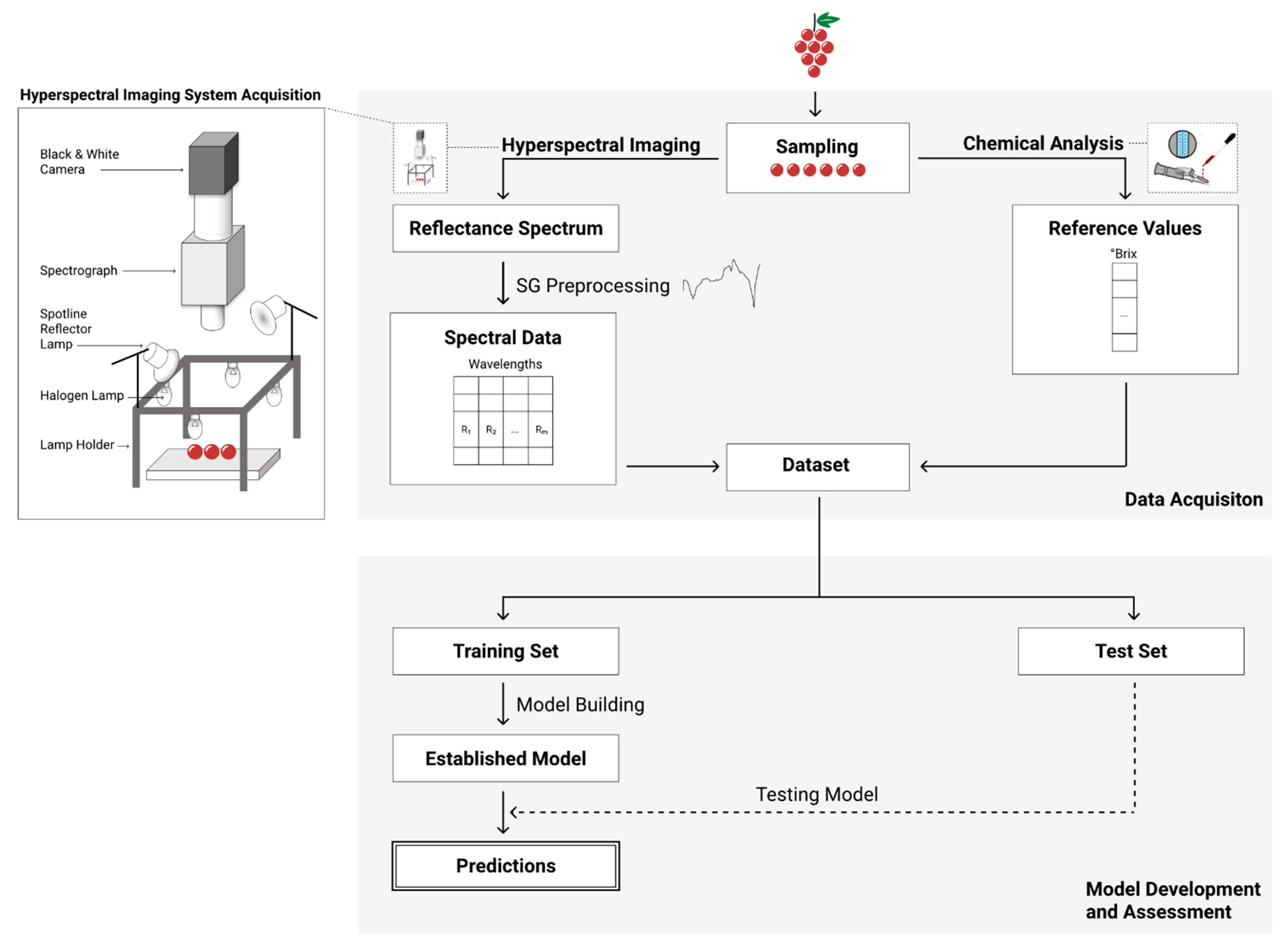
Figure 1 portrays the overall workflow followed in this study. The main steps are briefly described in the following subsections.

2.1. Samples Description

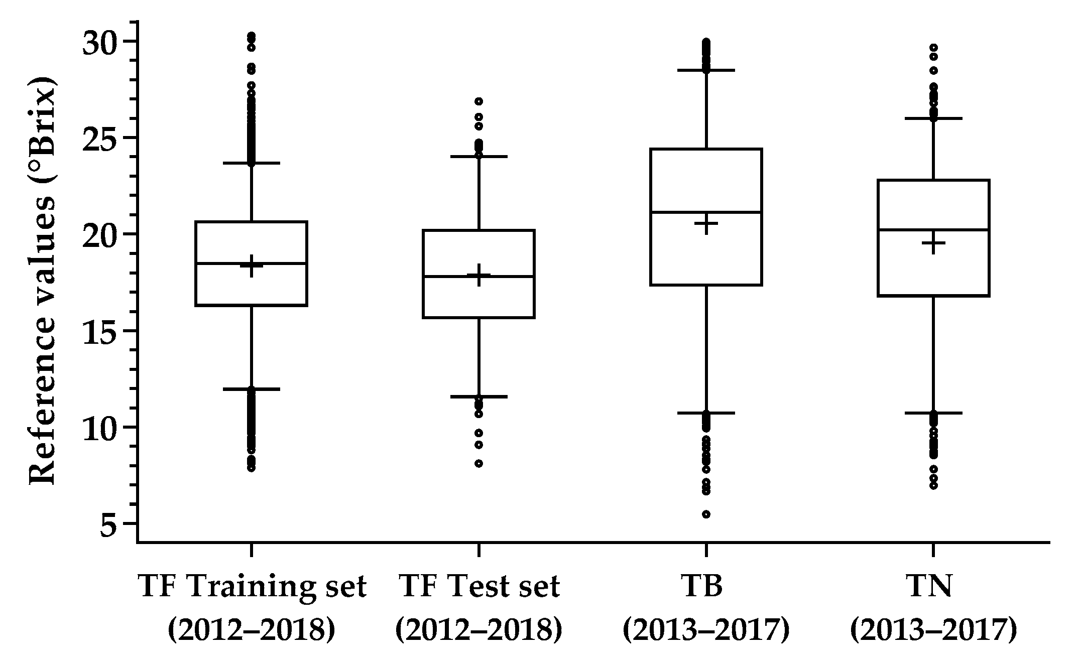
Three varieties widely used to produce Port wine in one of the oldest appellation regions of the world, the Portuguese Douro region, were selected to conduct this study: Touriga Franca (TF), Touriga Nacional (TN) and Tinta Barroca (TB). These grape varieties were selected due to their importance to the Porto wine industry, and were harvested from vineyards of Quinta do Bomfim, Pinhão (Portugal), in three different locations within the vineyard (from vines with small, medium and large vigor) and with two different sun expositions (sunny and shaded sides). Grape samples of TF were collected in 2012, 2013, 2014, 2016, 2017 and 2018 vintages, while TN and TB varieties were harvested in 2013, 2014, 2016 and 2017 vintages. All vintages and varieties were collected between the beginning of veraison and maturity, composing a total of 1748 samples for TF, 454 samples for TN and 463 samples for TB. TF samples were used to develop and test the predictive models while TN and TB were only used to test the generalization capacity of models created with TF for different varieties.

Each sample for each variety was composed of six (from 2012 to 2014 vintages) or twelve (from 2016 to 2018 vintages) grape berries randomly collected from a single bunch with their pedicel attached. This small number of grape berries per sample was used due to the practice of some wineries to select the best berries from each bunch for the production of high-quality wines [1,29]. The increase from six to twelve grape berries per sample was due to the fact that sometimes, depending on the variety, six grape berries may not be enough to obtain a representative sample for carrying out the conventional analysis. A line-scan hyperspectral image acquisition (described in Section 2.2) was performed using fresh grape samples and after imaging, and before conventional analysis, all samples were frozen at −18 °C.

2.2. Data Acquisition

Hyperspectral measurements were collected using the following hyperspectral imaging system acquisition (Figure 1): a hyperspectral camera, composed of a JAI Pulnix (JAI, Yokohama, Japan) black and white camera and a Specim Imspector V10E spectrograph (Specim, Oulu, Filand); lighting, using a lamp holder with 300 × 300 × 175 mm³ (length × width × height) that held four 20 W, 12 V halogen lamps and two 40 W, 220 V blue reflector lamps (Spotline, Philips, Eindhoven, The Netherlands). The halogen lamps were powered by continuous current power supplies to avoid light flickering and the reflector lamps were powered at only 110 V to reduce lighting and prevent camera saturation. The acquired images have a spatial resolution of 1040 × 1392 pixels, where 1040 pixels correspond to the wavelength channels, ranging between 380 and 1028 nm, with approximately 0.6 nm width for each channel. The 1392 pixels stand for the spatial dimension (one line over the samples) with approximately 110 mm of width. The distance between the camera and the sample base was set to 420 mm, and the camera was controlled with the Coyote software from JAI. All the hyperspectral measurements were done inside a semi-darkened room and at room temperature (20 °C). After image collection, the grape berries were identified and extracted using a threshold-based segmentation method.

Regarding the established lighting conditions (Figure 1), measurements were done in reflectance mode. To do so, it was necessary to determine the reflectance values, aiming to correct signal variations caused by the illumination and the hyperspectral camera. Reflectance is defined as the ratio between the total intensity of light reflected by a sample and the total intensity of light incident on the sample. To compute the intensity of light that illuminates the grape berries, a white reference target called Spectralon (Specim, Oulu, Filand) was used. Spectralon reflects almost 100% of the light that reaches its surface in the ultraviolet, visible and infra-red wavelengths. Thus, for a given wavelength, λ, and, due to the use of hyperspectral imaging, also for a certain position, x, the reflectance, R, is computed as:

$$R(x,\lambda )=\frac{GI(x,\lambda )-DI(x,\lambda )}{SI(x,\lambda )-DI(x,\lambda )}$$

(1)

where GI is the intensity of light reflected by the grape berries, SI the intensity of light coming from the white reference target and DI the dark current signal (electronic noise) associated to hyperspectral camera output acquired by keeping the camera shutter closed. The dark current signal depends on the camera electronics and must be subtracted from the grape berries and Spectralon intensities to avoid tampering in the determination of the reflectance values.

In the present work, the hyperspectral measurements for each sample were carried out along the berry “equator”, considering the pedicel as the pole, and for three different berry positions corresponding to berry rotations of approximately 120° between positions, allowing that the whole equator was imaged. In order to minimize the measurement noise, an accumulation of 32 hyperspectral images were acquired for SI(x, λ), DI(x, λ) and for each set of positions in GI(x, λ). The final hyperspectral images were obtained by averaging the 32 images and, after the identification of grape berries, the reflectance values were calculated through Equation (1). To create a unique reflectance spectrum for each sample, the reflectance spectra measured for all berries’ points were averaged over the spatial dimension and positions. Furthermore, to properly develop the predictive models, it was also necessary to determine the reference values for the sugar content, through conventional chemical analysis. In this work, for each analytical sample, the grapes were defrosted, crushed and the °Brix was then determined by refractometry [32].

After data acquisition, each acquired spectrum was paired with the reference measurements for the sugar contents to create the final datasets. Moreover, in order to handle undesirable physical phenomena in the spectra and to develop more parsimonious and stable predictive models, the spectral data was preprocessed using Savitzky–Golay first derivative. More information about the data acquisition process and measurement protocols are available in [1,18,22,29].

2.3. Predictive Methods

Four different approaches were considered in this work (RR, PLSR, NN and 1D CNN) for the predictive model. A brief description of these four approaches is provided below as more detailed descriptions are provided in the literature [1,18,29,33,34,35].

Ridge regression (RR) is a popular machine learning method that belongs to the class of penalized regression methods. It imposes a squared penalty (L²-norm) on the magnitude of the regression coefficients, constraining their magnitude to be low. The penalty term stabilizes the estimation of the coefficients, mitigating the effects of collinearity, overfitting, and improving model robustness. In this regard, the regression coefficients, $\left({\widehat{b}}_{\mathrm{RR}}\right)$, are obtained by solving the following optimization problem (2):

$${\widehat{b}}_{\mathrm{RR}}=\underset{b={[b_0\dots b_p]}^T}{\arg \min }\left\{{\displaystyle \sum _{i=1}^n{\left(y\left(i\right)-\widehat{y}\left(i\right)\right)}^2}+\gamma {\displaystyle \sum _{j=1}^p{b}_j^2}\right\}$$

(2)

where ${\displaystyle \sum _{j=1}^p{b}_j^2}$ is the squared L²-norm penalization, $y(i)$ is the ith observed response value, $\widehat{y}(i)$ is the corresponding model prediction and γ controls the bias-variance tradeoff, weighting the contribution of the classical least-squares term with the penalization term for the regression coefficient size. Suitable values of γ were selected through k-fold cross-validation in order to control the bias-variance tradeoff and impose an adequate penalization for maximum prediction accuracy [33].

Partial least squares regression (PLSR) is a method widely used in chemometrics and related areas, fitting into the class of latent variables. The basic assumptions of PLSR rely on the inference of new variables called latent variables (LV), corresponding to the projections of the input (X) and output (Y) sets of variables into new subspaces, where the covariance between X and Y is maximized [36]. The number of latent variables was chosen by minimizing the root mean squared error obtained through k-fold cross-validation. The maximum number of latent variables considered was set to eighty.

Artificial neural networks (NN) form another class of machine learning methods, consisting of parallel assemblies of non-linear mathematical units disposed in layers mimicking the function of neurons in the brain [37]. This method has the ability of learning from patterns that constitute the training set [38]. In this work we used a feedforward multilayer perceptron, composed of several layers of neurons interconnected by weights that store the knowledge acquired during the learning process [1]. During the training process, the weights are computed iteratively in order to minimize the deviations between the estimates and the reference sugar contents. Each iteration for weights adjustment is called an epoch. Furthermore, the neural networks were trained using the Levenberg–Marquardt algorithm [37], a backpropagation approach with a variable learning rate that is more efficient than the conventional algorithm approach. The training step was repeated for 100 different randomly generated initial weights and was stopped when the number of epochs with the lowest mean squared error for validation was achieved (known as early stopping). The hyperbolic tangent (non-linear function) and the identity (linear function) were the activation functions used to compute the hidden and output neurons, respectively. As the input data dimensionality of a neural network should be kept as low as possible to provide model parsimony and lower the risk of overfitting, principal component analysis (PCA) was applied to reduce the high dimensionality of the spectra. To find the optimal number of principal components, a range between one and eighty was tested. The procedure of k-fold cross-validation was also adopted for the development of the neural network model.

Convolutional neural networks (CNN), abbreviated as ConvNets herein, belong to the deep learning class of machine learning methods and have been applied in different research fields, notably for image classification. CNN models usually contain layers of 2D convolutional kernels [34]. However, in our approach, the sets of spectral data resulting from hyperspectral imaging procedure are one-dimensional (1D), which implies using a 1D kernel in the CNN instead of the commonly employed 2D or 3D kernels. The customized 1D CNN (see Figure 2) was built in Python using keras v.2.2.4 package, fed with a one-dimensional input (1040 × 1) and followed by two one-dimensional convolutional layers. Twenty 1D filters were used in each convolutional layer with sixteen and eight 1D kernel sizes, respectively, using a rectified linear unit (ReLU) as non-linear activation function. This way we aim to capture first the coarse spectral connections and then refine them. Pooling layers are usually employed after the convolutional layers to reduce the dimensionality of feature maps. However, they are not always used in problems dealing with one-dimensional spectral data [39,40], being simply replaced in these circumstances by a convolutional layer with increased stride and usually without significant loss in accuracy [39,41]. This modification also simplifies the network structure. In this work, we adopt the strategy of not using pooling layers, building a simpler 1D CNN (i.e., with fewer layers) to derive the model. Thus, the ‘same’ padding was used and the stride value of the first convolutional layer was set to one and the second to eight. The outputs arising from the final convolutional layer were flattened and a dropout layer was added to avoid overfitting before connecting to a fully connected dense layer with a ReLU activation function. The output layer was a single dense neuron with a linear activation function. The training process was done using the Adadelta optimizer [42] and the convolutional weights were initiated using ‘Glorot uniform’ initialization [43] and computed, iteratively, for 300 epochs. Batch size was set to 64. To obtain the model, an early stopping was included and the mean squared error was defined as loss function.

RR, PLSR and NNs computations were conducted in the MATLAB R2019b environment (MathWorks, Inc., Natick, Massachusetts, United States).

2.4. Model Development and Assessment

In order to develop, assess and compare the predictive ability of the different estimated models, the data (spectral and the respective reference measurements) were split into training and independent test sets, using a stratified scheme based on the response percentiles. To perform this step, the data for each Touriga Franca vintage (from 2012 to 2018) was grouped into 5 intervals according to the following sugar content percentiles: 20th, 40th, 60th and 80th. In each group of percentile intervals, 10% of samples were reserved for the independent test set and the remaining were used for model training. The final datasets (training and independent test sets) were formed by collecting the respective TF samples partitioned for each vintage. This independent test set was used in the test phase to assess the prediction performance of each method in order to ensure an unbiased measurement of the model’s robustness.

Regarding the ridge regression, partial least square and neural networks methods, a stratified k-fold cross-validation approach was used during model training in order to select the suitable hyperparameter(s) mentioned in Section 2.3 for each predictive method. This was done using 9-fold cross-validation wherein the data was partitioned in nine folds, eight used for training and one for validation. Training was repeated nine times using a different validation fold each time. The cross-validation results presented in this work consist of the average of the results obtained in the nine folds when they were used for validation. The final models were trained using the nine folds and the respective best hyperparameter(s) obtained by k-fold cross-validation approach. For the development of the proposed one-dimensional convolutional neural network architecture, unlike the other three methods, the training set was divided into calibration and validation sets using the same stratified scheme based on percentiles explained above, with 10% of TF samples reserved for validation set. The calibration set was used to estimate the model and the validation set was applied to tune the internal parameters (weights and biases).

The performance of each machine learning method (RR, PLS, NN and 1D CNN) was assessed and compared using the independent test set formed with all samples of TF vintages not employed during the training stage, and the model’s generalization ability was evaluated through all samples of TN and TB varieties (different years and varieties) as independent test sets.

Table 2. Outline of the scenarios performed in the sections below (TF—Touriga Franca; TN—Touriga Nacional; TB—Tinta Barroca).

Training Set	Independent Test Sets	Section
TF 2012 to 2018	TF 2012 to 2018	Section 3.2
	TN 2013 to 2017	Section 3.3
	TB 2013 to 2017

provides detailed information about the training and independent test sets created to conduct the comparison.

The root mean squared error (RMSE) was used as an evaluation criterion of the model and to compare the proposed approaches.

3. Results and Discussion

3.1. Results for the Sugar Chemical Analysis

A summary of the descriptive statistics obtained by conventional techniques for sugar content in each vintage and for all varieties is presented in

Table 3. Summary of the descriptive statistics for the reference measurements of sugar contents by variety and vintage.

Variety and Vintage	N a	Mean	SD b	95% CI	Min c	Max d	Range (Max–Min)	Q1 e	Median	Q3 f	Percentiles
											5th	95th
TF 2012	240	16.93	3.34	(16.50; 17.35)	9.06	24.72	15.66	14.92	17.06	19.07	11.10	22.58
TF 2013	81	19.40	3.58	(18.60; 20.18)	8.10	25.00	16.9	17.85	20.00	21.74	13.40	23.94
TF 2014	120	13.55	3.66	(12.89; 14.21)	7.87	25.66	17.79	10.77	13.00	15.57	9.04	21.11
TF 2016	407	17.83	2.61	(17.57; 18.08)	10.07	26.03	15.96	16.07	17.54	19.47	14.07	22.42
TF 2017	540	19.86	3.36	(19.57; 20.14)	10.94	30.08	19.14	17.82	20.34	22.18	13.14	24.77
TF 2018	360	19.01	2.68	(18.72; 19.28)	11.92	30.26	18.34	17.37	18.65	20.38	15.27	23.76
TN 2013	60	23.25	2.44	(22.62; 23.88)	17.20	27.20	10.00	21.56	23.84	24.90	17.80	26.26
TN 2014	118	15.67	4.35	(14.88; 16.46)	6.95	24.86	17.91	12.67	15.87	19.06	8.67	22.86
TN 2016	132	19.37	2.90	(18.87; 19.87)	12.94	24.70	11.76	16.98	19.49	21.61	14.40	24.02
TN 2017	144	21.28	3.87	(20.64; 21.92)	11.61	29.66	18.05	18.86	21.44	23.86	14.41	27.20
TB 2013	82	22.30	4.39	(21.33; 23.26)	11.40	29.45	18.05	19.47	23.37	25.40	14.00	28.11
TB 2014	120	15.70	4.79	(14.83; 16.57)	6.67	28.55	21.88	11.93	15.14	19.43	8.44	23.38
TB 2016	143	21.21	3.98	(20.55; 21.87)	5.48	29.70	24.22	18.29	21.10	24.30	15.29	27.70
TB 2017	118	23.51	4.27	(22.73; 24.29)	10.41	29.95	19.54	20.94	23.62	27.15	15.73	29.46

^a Number of samples. ^b Standard deviation. ^{c, d} Minimum and maximum values. ^{e, f} 1st and 3rd Quartile or 25th and 75th percentiles, respectively.

. These enological values were used as reference values to create and test the proposed models. From Table 3, it is possible to observe differences between varieties for the same vintage, and differences between vintages for the same variety, which may create difficulties in the prediction of new samples not employed in the training stages. The ranges between the maximum and minimum are due to the ripening of berries that were collected from the beginning of the veraison until the date of harvest. Furthermore, the differences in terroir combined with the constant climatic variations over the years show a substantial impact in the grape ripening stage within a vintage and between vintages. The mean standard deviation and percentiles vary widely between vintages and varieties but, in general, TB variety presents the larger variability. Overall, within varieties and for each vintage, TF values range from 7.87 up to 30.26 °Brix, while in TN and TB have minimums of 6.95 and 5.48 °Brix and the maximums of 29.66 and 29.95 °Brix, respectively. For more information about the descriptive statistics of the datasets used in the following subsections, see the boxplot presented in Appendix A (Figure A1).

3.2. Comparison of Predictive Models in the TF Samples Testing Scenario

In this stage, we aimed to evaluate and compare the prediction performance of RR, PLS, NN and 1D CNN models using the independent test set created with different vintages of TF (the same variety as in the training stage).

Table 4. Results obtained by the four classes of machine learning methods for validation and test sets, using the Touriga Franca variety.

Model	Validation Set		Independent Test Set
	R2	RMSECV a/RMSEV b (°Brix)	R2	RMSEP c (°Brix)
RR	0.84 1	1.40 1	0.83	1.44
PLS	0.84 1	1.41 1	0.83	1.47
NN	0.91 1	1.10 1	0.89	1.14
1D CNN	0.94	0.93	0.92	0.97

^a Root mean square error of cross-validation. ^b Root mean square error of validation. ^c Root mean square error of prediction. ¹ Results obtained by 9-fold cross-validation.

summarizes the results obtained with validation set (9-fold cross-validation and validation as described in Section 2.4) and independent test set, regarding the four ML classes considered. The best neural network structure obtained by k-fold cross-validation had one hidden layer with four neurons and 54 PCs for inputs while the best performance for PLS was obtained with 35 latent variables. Concerning RR, the best performance was found with a γ value of 0.1. From the analysis of Table 4, it is possible to identify the one-dimensional convolutional neural network as the best predictive method to predict sugar content in the current scenario, obtaining the lowest RMSE values. The validation results obtained with each machine learning method presented a root mean square error of 1.40, 1.41, 1.10 and 0.93 °Brix for RR, PLS, NN and 1D CNN, respectively; for the independent test set the RMSE values were 1.45, 1.47, 1.14 and 0.97 °Brix, respectively.

Figure 3 depicts the histograms of absolute errors (AE) for each predictive method, regarding the independent test set. The percentage of samples with AE smaller than 0.5 °Brix is 29.14% for RR, 30.86% for PLS, 35.43% for NN and 47.43% for 1D CNN. With AE smaller than 1.0 °Brix is 54.43%, 54.29%, 73.72% and 74.29%, respectively. Regarding AE smaller than 1.5 °Brix and also lesser than 2.0 °Brix, the percentage of samples is 79.43% and 85.15% for RR; 71.43% and 82.86% for PLS; 85.15% and 90.86% for NN; and 88.58% and 96.01% for 1D CNN, respectively.

In order to evaluate if there are statistical differences between the absolute errors of predictions across each pair of methods, a paired t-test with a significance level of 0.05 was computed (see

Table 5. Paired t-test to evaluate differences between the absolute errors of predictions for each pair of methods applied (α = 0.05) in the 175 samples of the independent test set.

Methods	Mean Difference	p-Value
RR-PLS	−0.07	0.11
RR-NN	0.20	<0.01
RR-1D CNN	0.35	<0.001
PLS-NN	0.27	<0.001
PLS-1D CNN	0.42	<0.001
NN-1D CNN	0.15	<0.001

). Through the analysis of this table, it is possible to observe that the means of absolute error for NN and 1D CNN are significantly different from the other two methods and differ significantly between them. Thus, although NN has a similar percentage of samples for absolute errors between 0.5 and 1.5 °Brix, 1D CNN present the best overall performance.

The scientific literature about the training and testing of models with more than one vintage is practically nonexistent, and can only be found in a few references [19,22]. In [22], samples from three different vintages and same location were used to train and test a support vector regression (SVR) algorithm, revealing a RMSEP value of 1.41 °Brix; in [19], a modified partial least squares (MPLS) regression algorithm was implemented to data gathered between 2006 and 2008, obtaining a RMSECV value of 1.0 °Brix. However, [19] used a large number of berries per sample (whole bunches), which reduces the variability in both the reflectance spectra and the reference values measured for sugar content, making the prediction problem easier. The predictions obtained with 1D CNN are more accurate than those reported in these references, while for the remaining methods the results are in accordance with [22].

3.3. Assessing the Generalization Ability: Testing with Different Varieties

The study of the model’s generalization ability was performed for the four models developed in Section 3.2. Thus, two new independent test sets (with different varieties and vintages, TN and TB) not employed during training, as described in Section 2.4, were used to assess the generalization capacity of each model established in Section 3.2. The results obtained with the new independent test sets and for each machine learning method are summarized in

Table 6. RMSEP values for sugar content when independent test sets with different varieties/vintages are applied in the previously established models to evaluate and compare their generalization ability.

Independent Test Sets	N a	RMSEP (°Brix)
		RR	PLS	NN	1D CNN
TN 2013 to 2017	454	2.59	2.22	1.45	1.15
TB 2013 to 2017	463	3.12	3.09	1.75	1.31

^a Number of samples in the independent test set.

.

Regarding each model’s generalization ability, it is possible to observe a decrease in the performance of the models, with higher RMSE values in the independent test sets for TN and TB varieties compared to the results obtained for the TF test set (Table 4). Nevertheless, convolutional neural networks present the best predictions for these two scenarios, obtaining the lowest RMSEP. Also, from the analysis of Table 6, it can be denoted that the models generalized better for samples of TN variety and worse for samples of TB variety. This might be related to the different distribution presented in Table 3 and Figure A1 (Appendix A), in which, within vintages, TB samples present a larger standard deviation when compared with the other varieties from the same vintage. Following the same procedure of Section 3.2, a paired t-test, with a significance level of 0.05, was carried out to investigate statistical differences between the absolute errors of predictions in the new independent test sets (see

Table 7. Paired t-test to evaluate differences between the absolute errors of predictions for each pair of methods, regarding the model’s generalization ability (α = 0.05).

Varieties/Vintages	Methods	Mean Difference	p-Value
TN 2013 to 2017	RR-PLS	0.27	<0.001
	RR-NN	0.90	<0.001
	RR-1D CNN	1.12	<0.001
	PLS-NN	0.62	<0.001
	PLS-1D CNN	0.85	<0.001
	NN-1D CNN	0.23	<0.001
TB 2013 to 2017	RR-PLS	0.04	0.09
	RR-NN	1.21	<0.001
	RR-1D CNN	1.56	<0.001
	PLS-NN	1.17	<0.001
	PLS-1D CNN	1.52	<0.001
	NN-1D CNN	0.35	<0.001

). This table clearly discloses the one-dimensional convolutional neural network as the most suitable approach for generalization tests using different vintages and varieties, being the method that most differs significantly from the others, showing the smallest RMSEP values.

Furthermore, since NN demonstrated to be the second method with the best performance, a comparison between both NN and 1D CNN was carried out, as illustrated in Figure 4, taking into account the predictions obtained for the independent test set composed by all samples of TN and TB plus the 10% of all samples of TF used as independent test set in Section 3.2. Through the interpretation of the results, we can see that 1D CNN shows a better performance than NN. Besides, the p-value obtained by the paired t-test showed that the means for each independent test set differ significantly (p-value < 0.001).

One of the strengths of deep learning and consequently the proposed 1D CNN, is the ability to automatically perform feature extraction, which is a fundamental procedure in machine learning to improve the model accuracy. As mentioned before, PCA was used to reduce the input dimensionality of the neural network; however, for the development of the 1D CNN model, all 1040 wavelengths were considered as feature input. Besides, despite the enormous amount of data generally needed to train deep learning methods, the results presented here provide good insights into the characteristics of the relationship between this methodology (hyperspectral imaging + 1D CNN) and the sugar content as the enological parameter. Nevertheless, the overall performance achieved with neural networks was indeed very satisfactory and with the prediction errors in an acceptable range, indicating that this can be a good choice to predict sugar content in the current scenario, and for the future addition of new features.

Concerning the scientific literature for the prediction of sugar content, there is only one work [22] that tackles the model’s generalization ability, taking into consideration different varieties not employed in the training. In [22] the generalization capacity of a SVR model was assessed using samples of TN and TB varieties from 2013 vintage, which revealed RMSE values of 2.44 and 3.44 °Brix, respectively. Thus, the RMSE values obtained in the present work (Table 6) are lower than [22] those for 1D CNN and NN, but similar for RR and PLS methods.

4. Conclusions

In the present work, we propose an approach that lays the groundwork for the development of an on-the-fly non-invasive sensing methodology for predicting and monitoring the key enological parameters of Port wine grape berries that are essential for their ripeness assessment.

Four different machine learning methods (ridge regression, partial least squares, neural networks and convolutional neural networks) were developed and compared for predicting the sugar content in grapes, one of the parameters most related to grape maturity. This comparison focused on the generalization ability for different vintages and varieties not employed in the training model. The prediction errors obtained by each method were within acceptable ranges, and as a result, the general performance achieved was indeed highly satisfactory in terms of robustness. Furthermore, these results reveal that the proposed 1D CNN architecture can be successfully applied to estimate sugar content of wine grape berries, achieving a better performance rate when compared with the other three methods of ridge regression, partial least squares and neural networks.

Additionally, this study shows that the differences in terroir and grape varieties have a considerable impact in the grape ripening stage within and between vintages and, consequently, on the robustness of the predictive models. Nevertheless, the combination of hyperspectral imaging technology with appropriate machine learning approaches proved to be a competitive candidate for the development of a powerful tool for fast, non-destructive and non-invasive evaluation of grape quality, and consequently, a potential tool to achieve desired wine properties and quality standards. In particular, the results obtained in the present work are promising to accurately measure the sugar content of wine grapes during ripening, providing important information to adapt the procedure defined at the laboratory level (laboratory-acquired data) to an on-the-fly non-invasive sensing approach. Furthermore, these results suggest that the increase of the number of training samples will further improve the robustness of the prediction models, making its use irrespective of the specific vintage year. The addition of pooling layers to the 1D CNN architecture should also be subjected to future research in order to compare its performance with the current architecture and verify whether or not the use of pooling layers can bring more predictive power to the problem. Finally, it is important in future research to perform field hyperspectral data acquisition to upscale these models at real conditions.

References

1. Fernandes, A.M.; Franco, C.; Mendes-Ferreira, A.; Mendes-Faia, A.; da Costa, P.L.; Melo-Pinto, P. Brix, pH and anthocyanin content determination in whole Port wine grape berries by hyperspectral imaging and neural networks. Comput. Electron. Agric. 2015, 115, 88–96. [Google Scholar] [CrossRef]
2. Janik, L.J.; Cozzolino, D.; Dambergs, R.; Cynkar, W.; Gishen, M. The prediction of total anthocyanin concentration in red-grape homogenates using visible-near-infrared spectroscopy and artificial neural networks. Anal. Chim. Acta 2007, 594, 107–118. [Google Scholar] [CrossRef]
3. Cao, F.; Wu, D.; He, Y. Soluble solids content and pH prediction and varieties discrimination of grapes based on visible–near infrared spectroscopy. Comput. Electron. Agric. 2010, 71, S15–S18. [Google Scholar] [CrossRef]
4. Agati, G.; D’Onofrio, C.; Ducci, E.; Cuzzola, A.; Remorini, D.; Tuccio, L.; Lazzini, F.; Mattii, G. Potential of a multiparametric optical sensor for determining in situ the maturity components of red and white vitis vinifera wine grapes. J. Agric. Food Chem. 2013, 61, 12211–12218. [Google Scholar] [CrossRef] [PubMed]
5. Ghozlen, N.B.; Cerovic, Z.G.; Germain, C.; Toutain, S.; Latouche, G. Non-destructive optical monitoring of grape maturation by proximal sensing. Sensors 2010, 10, 10040–10068. [Google Scholar] [CrossRef]
6. Baiano, A.; Terracone, C.; Peri, G.; Romaniello, R. Application of hyperspectral imaging for prediction of physico-chemical and sensory characteristics of table grapes. Comput. Electron. Agric. 2012, 87, 142–151. [Google Scholar] [CrossRef]
7. Maldonado, A.I.L.; Rodriguez-Fuentes, H.; Contreras, J.A.V. Hyperspectral Imaging in Agriculture, Food and Environment; IntechOpen: London, UK, 2018; ISBN 9781789232905. [Google Scholar]
8. Rady, A.M.; Guyer, D.E.; Kirk, W.; Donis-González, I.R. The potential use of visible/near infrared spectroscopy and hyperspectral imaging to predict processing-related constituents of potatoes. J. Food Eng. 2014, 135, 11–25. [Google Scholar] [CrossRef]
9. Chen, Q.; Zhang, C.; Zhao, J.; Ouyang, Q. Recent advances in emerging imaging techniques for non-destructive detection of food quality and safety. TrAC-Trends Anal. Chem. 2013, 52, 261–274. [Google Scholar] [CrossRef]
10. Sun, D.W. Hyperspectral Imaging for Food Quality Analysis and Control; Elsevier: Amsterdam, The Netherlands, 2010; ISBN 9780123747532. [Google Scholar]
11. Prats-Montalbán, J.M.; de Juan, A.; Ferrer, A. Multivariate image analysis: A review with applications. Chemom. Intell. Lab. Syst. 2011, 107, 1–23. [Google Scholar] [CrossRef]
12. Gowen, A.A.; O’Donnell, C.P.; Cullen, P.J.; Downey, G.; Frias, J.M. Hyperspectral imaging—An emerging process analytical tool for food quality and safety control. Trends Food Sci. Technol. 2007, 18, 590–598. [Google Scholar] [CrossRef]
13. Hall, A.; Lamb, D.W.; Holzapfel, B.; Louis, J. Optical remote sensing applications in viticulture—A review. Aust. J. Grape Wine Res. 2002, 8, 36–47. [Google Scholar] [CrossRef]
14. Geraudie, V.; Roger, J.M.; Ojeda, H. Développement d’un appareil permettant de prédire la maturité du raisin par spectroscopie proche infrarouge (PIR). Rev. Fr. D’oenol. 2010, 240, 2–8. [Google Scholar]
15. Herrera, J.; Guesalaga, A.; Agosin, E. Shortwave–near infrared spectroscopy for non-destructive determination of maturity of wine grapes. Meas. Sci. Technol. 2003, 14, 689. [Google Scholar] [CrossRef]
16. Larrain, M.; Guesalaga, A.R.; Agosin, E. A Multipurpose Portable Instrument for Determining Ripeness in Wine Grapes Using NIR Spectroscopy. Instrum. Meas. IEEE Trans. 2008, 57, 294–302. [Google Scholar] [CrossRef]
17. Fernandes, A.; Gomes, V.; Melo-Pinto, P. A Review of the Application to Emergent Subfields in Viticulture of Local Reflectance and Interactance Spectroscopy Combined with Soft Computing and Multivariate Analysis BT—Soft Computing for Sustainability Science; Cruz Corona, C., Ed.; Springer International Publishing: Cham, Switzerland, 2018; pp. 87–115. ISBN 978-3-319-62359-7. [Google Scholar]
18. Gomes, V.M.; Fernandes, A.M.; Faia, A.; Melo-Pinto, P. Comparison of different approaches for the prediction of sugar content in new vintages of whole Port wine grape berries using hyperspectral imaging. Comput. Electron. Agric. 2017, 140, 244–254. [Google Scholar] [CrossRef]
19. González-Caballero, V.; Pérez-Marín, D.; López, M.-I.; Sánchez, M.-T. Optimization of NIR Spectral Data Management for Quality Control of Grape Bunches during On-Vine Ripening. Sensors 2011, 11, 6109–6124. [Google Scholar] [CrossRef] [Green Version]
20. Hernández-Hierro, J.M.; Nogales-Bueno, J.; Rodríguez-Pulido, F.J.; Heredia, F.J. Feasibility Study on the Use of Near-Infrared Hyperspectral Imaging for the Screening of Anthocyanins in Intact Grapes during Ripening. J. Agric. Food Chem. 2013, 61, 9804–9809. [Google Scholar] [CrossRef]
21. Nogales-Bueno, J.; Hernández-Hierro, J.M.; Rodríguez-Pulido, F.J.; Heredia, F.J. Determination of technological maturity of grapes and total phenolic compounds of grape skins in red and white cultivars during ripening by near infrared hyperspectral image: A preliminary approach. Food Chem. 2014, 152, 586–591. [Google Scholar] [CrossRef] [PubMed]
22. Silva, R.; Gomes, V.; Mendes-Faia, A.; Melo-Pinto, P. Using support vector regression and hyperspectral imaging for the prediction of oenological parameters on different vintages and varieties ofwine grape berries. Remote Sens. 2018, 10, 312. [Google Scholar] [CrossRef] [Green Version]
23. Arana, I.; Jarén, C.; Arazuri, S. Maturity, variety and origin determination in white grapes (Vitis Vinifera L.) using near infrared reflectance technology. J. Near Infrared Spectrosc. 2005, 13, 349–357. [Google Scholar] [CrossRef]
24. Chen, S.; Zhang, F.; Ning, J.; Liu, X.; Zhang, Z.; Yang, S. Predicting the anthocyanin content of wine grapes by NIR hyperspectral imaging. Food Chem. 2015, 172, 788–793. [Google Scholar] [CrossRef]
25. Cozzolino, D.; Cynkar, W.; Janik, L.; Dambergs, R.; Francis, L.; Gishen, M. Measurement of colour, total soluble solids and pH in whole red grapes using visible and near infrared spectroscopy: [poster summary]. In Proceedings of the 12th Australian Wine Industry Technical Conference, Melbourne, Australia, 24–29 July 2004; pp. 334–335. [Google Scholar]
26. dos Santos Costa, D.; Oliveros Mesa, N.F.; Santos Freire, M.; Pereira Ramos, R.; Teruel Mederos, B.J. Development of predictive models for quality and maturation stage attributes of wine grapes using vis-nir reflectance spectroscopy. Postharvest Biol. Technol. 2019, 150, 166–178. [Google Scholar] [CrossRef]
27. Fadock, M.; Brown, R.B.; Reynolds, A.G. Visible-Near Infrared Reflectance Spectroscopy for Nondestructive Analysis of Red Wine Grapes. Am. J. Enol. Vitic. 2016, 67, 38–46. [Google Scholar] [CrossRef]
28. Ferrer-Gallego, R.; Hernández-Hierro, J.M.; Rivas-Gonzalo, J.C.; Escribano-Bailón, M.T. Determination of phenolic compounds of grape skins during ripening by NIR spectroscopy. LWT-Food Sci. Technol. 2011, 44, 847–853. [Google Scholar] [CrossRef] [Green Version]
29. Gomes, V.; Fernandes, A.; Martins-Lopes, P.; Pereira, L.; Mendes Faia, A.; Melo-Pinto, P. Characterization of neural network generalization in the determination of pH and anthocyanin content of wine grape in new vintages and varieties. Food Chem. 2017, 218, 40–46. [Google Scholar] [CrossRef] [PubMed]
30. Gomes, V.; Fernandes, A.; Faia, A.; Pinto, P.M. A Comparison of Neural Networks and Partial Least Squares for Estimation of Sugar Content in Wine Grape Berries Using Hyperspectral Imaging. In Proceedings of the International Conference on Computer Science and Environmental Engineering (Csee 2015), Beijing, China, 17–18 May 2015. [Google Scholar]
31. Gomes, V.; Rendall, R.; Mendes-Ferreira, A.; Reis, M.; Melo-Pinto, P. Wine grape quality assessment using hyperspectral imaging—A predictive analytics comparison framework. In Proceedings of the International Congress on Grapevine and Wine Sciences, Logroño, Spain, 7–9 November 2018; p. 46. [Google Scholar]
32. Organisation International de la Vigne e du Vin Recueil des Méthodes Internationales D’analyse des vins et des Mouts; OIV: Paris, France, 2006.
33. Rendall, R.; Reis, M.S. Which regression method to use? Making informed decisions in “data-rich/knowledge poor” scenarios—The Predictive Analytics Comparison framework (PAC). Chemom. Intell. Lab. Syst. 2018, 181, 52–63. [Google Scholar] [CrossRef]
34. Albawi, S.; Mohammed, T.A.; Al-Zawi, S. Understanding of a convolutional neural network. In Proceedings of the 2017 International Conference on Engineering and Technology, ICET 2017, Antalya, Turkey, 21–23 August 2017. [Google Scholar]
35. Srinivasamurthy, R.S. Understanding 1D Convolutional Neural Networks Using Multiclass Time-Varying Signals. Ph.D. Thesis, Clemson University, Clemson, SC, USA, 2018. [Google Scholar]
36. Wold, S.; Sjöström, M.; Eriksson, L. PLS-regression: A basic tool of chemometrics. Chemom. Intell. Lab. Syst. 2001, 58, 109–130. [Google Scholar] [CrossRef]
37. Bishop, C.M. Neural Networks for Pattern Recognition; Clarendon Press, Oxford University Press: Oxford, UK, 1995; ISBN 9780198538646. [Google Scholar]
38. Marini, F.; Bucci, R.; Magrì, A.L.; Magrì, A.D. Artificial neural networks in chemometrics: History, examples and perspectives. Microchem. J. 2008, 88, 178–185. [Google Scholar] [CrossRef]
39. Acquarelli, J.; van Laarhoven, T.; Gerretzen, J.; Tran, T.N.; Buydens, L.M.C.; Marchiori, E. Convolutional neural networks for vibrational spectroscopic data analysis. Anal. Chim. Acta 2017. [Google Scholar] [CrossRef] [PubMed] [Green Version]
40. Yan, X.; Fu, H.; Zhang, S.; Qu, H. Combining convolutional neural networks and in-line near-infrared spectroscopy for real-time monitoring of the chromatographic elution process in commercial production of notoginseng total saponins. J. Sep. Sci. 2020, 43, 663–670. [Google Scholar] [CrossRef] [PubMed]
41. Springenberg, J.T.; Dosovitskiy, A.; Brox, T.; Riedmiller, M. Striving for simplicity: The all convolutional net. In Proceedings of the 3rd International Conference on Learning Representations, ICLR 2015—Workshop Track Proceedings, San Diego, CA, USA, 7–9 May 2015. [Google Scholar]
42. Zeiler, M.D. ADADELTA: An Adaptive Learning Rate Method. arXiv 2012, arXiv:1212.5701. [Google Scholar]
43. Glorot, X.; Bengio, Y. Understanding the difficulty of training deep feedforward neural networks. In Proceedings of the Thirteenth International Conference on Artificial Intelligence and Statistics, Sardinia, Italy, 13–15 May 2010; Volume 9, pp. 249–256. [Google Scholar]
Figure 1. Graphical representation of the experimental procedure adopted in the current work.
Processes 09 01241 g001
Figure 2. One−dimensional convolutional neural network architecture.
Processes 09 01241 g002
Figure 3. Histograms of absolute error for the TF independent test set: (a) ridge regression; (b) partial least squares; (c) neural network; (d) one-dimensional convolutional neural network.
Processes 09 01241 g003
Figure 4. Prediction results of the independent test set with samples of the varieties TF (blue points), TN (green points) and TB (orange points) when applied into the created models with TF samples, regarding: (a) neural network; (b) one-dimensional convolutional neural network.
Processes 09 01241 g004