Bayesian Analysis for Cardiovascular Risk Factors in Ischemic Heart Disease

Abstract

Ischemic heart disease (or Coronary Artery Disease) is the most common cause of death in various countries, characterized by reduced blood supply to the heart. Statistical models make an impact in evaluating the risk factors that are responsible for mortality and morbidity during IHD (Ischemic heart disease). In general, geometric or Poisson distributions can underestimate the zero-count probability and hence make it difficult to identify significant effects of covariates for improving conditions of heart disease due to regional wall motion abnormalities. In this work, a flexible class of zero inflated models is introduced. A Bayesian estimation method is developed as an alternative to traditionally used maximum likelihood-based methods to analyze such data. Simulation studies show that the proposed method has a better small sample performance than the classical method, with tighter interval estimates and better coverage probabilities. Although the prevention of CAD has long been a focus of public health policy, clinical medicine, and biomedical scientific investigation, the prevalence of CAD remains high despite current strategies for prevention and treatment. Various comprehensive searches have been performed in the MEDLINE, HealthSTAR, and Global Health databases for providing insights into the effects of traditional and emerging risk factors of CAD. A real-life data set is illustrated for the proposed method using WinBUGS.

1. Introduction

Throughout the world, heart disease is the biggest cause of death in both men and women [1]. One can die from heart disease about every minute in the United States alone, and one in every four deaths is associated with heart disease [2]. Cardiovascular Diseases (CVDs) lead the causes of morbidity and mortality worldwide, about 422.7 million prevalent cases and 17.92 million deaths (one-third of all deaths) estimated recently for the global burden of CVDs [3]. CAD is one of the most important causes of cardiovascular morbidity and mortality, with a global estimation of 110.55 million prevalent cases and 8.92 deaths, which makes coronary artery disease the leading cause of death in the world [3]. It is a common problem in public health and increases health costs. Invasive coronary arteriography (ICA), the gold standard procedure for diagnosing CAD, has been used in cases of clinical practice. The ICA procedure is an excessive medical treatment that is able to reduce misdiagnoses of CAD in patients. In a current report, only 41% of patients without known diseases who underwent ICA had obstructive CAD. Pre-test probability (PTP) estimates for obstructive CAD limit the risk of unsuitable examination, which is of utmost importance for health care systems. Recently, the DFM (Diamond Forrester model) and DCM (Duke Clinical Score) models [4,5] showed these facts. Additionally, NICE (National Institute for Health and Care Excellence, in UK) has also favoured the identification of chest pain (anginal) or abnormal resting electrocardiograms (ECGs) in a simple way, which is responsible for CAD testing by CCTA, i.e., coronary computed tomography angiography [6]. CCTA is a noninvasive method that can help to determine if plaque buildup has narrowed the coronary arteries. The European Society of Cardiology (ESC) updated guideline determines PTP from the stratified prevalence of CAD in a contemporary cohort instead of recurring in a prediction model as in the past. However, better strategies are required because half of the people who go through this expensive procedure do not need it [7]. The European and American guidelines have recently placed great importance on the initial risk stratification of suspected CAD to avoid unwarranted examinations. It is a pathological process that is characterized by atherosclerotic plaque accumulation in the epicardial arteries, either obstructive or non-obstructive. This process modification can be made by lifestyle adjustments, pharmacological therapies, and invasive interventions designed to achieve disease stabilization or regression. Moreover, CAD has long, stable periods. However, this disease can also become unstable at any time, typically due to an acute atherothrombotic event that is caused by plaque rupture or erosion. It is most often progressive and chronic. Therefore, this disease is very serious even in clinically apparently silent periods. The dynamic nature of the CAD process provides the results in different clinical presentations, which are categorized as follows [8]: (i) acute coronary syndromes (ACS) or (ii) chronic coronary syndromes (CCS).

Heart disease is a general term that means that the heart is not working normally. A person can have heart disease but not feel any illness. However, some people with heart disease have symptoms (pain in chest, trouble for breathing, palpitations, swelling of feet or legs, cyanosis, or feeling weak due to the body and brain not getting enough blood to supply them with oxygen). Nowadays, Coronary Artery Disease (CAD) is the most common heart disease in the World. CAD is also known as ischemic heart disease (IHD). It normally happens when cholesterol accumulates on the arterial walls and creates plaques. This is known as atherosclerosis. The arteries become narrow and reduce blood flow to the heart. Sometimes, a clot can obstruct the delivery of blood to the heart muscle. If blood vessels connected to the heart become very narrow or somehow blood vessels are blocked partially or completely, then blood cannot flow through them normally. As a result, muscles cannot work in a normal capacity to supply requisite amounts of blood to the heart muscle. The heart muscle becomes sick and weak; in fact, it can even die if blood flow stops. There are four primary coronary arteries detected on the heart’s surface: (i) right main coronary artery, (ii) left main coronary artery, (iii) left circumflex artery, and (iv) left anterior descending artery. These arteries are responsible for bringing oxygen and nutrient-rich blood to the heart. A healthy heart can move approximately 3000 gallons of blood daily throughout a human body according to the Cleveland Clinic. Generally, in the case of CAD patients with hypertension, the target of blood pressure is less than 140/90 mm Hg, which is reasonable for the secondary prevention of cardiovascular events. A lower target of $130/80$ mm Hg may be acceptable in some of these patients with stroke, transient ischemic attack (TIA), previous myocardial infarction (MI), or CAD risk equivalents [9].

It happens that stable CAD is commonly caused by a narrowing of the atherosclerotic coronary artery. It is characterized by a series of reversible myocardial demands or supply mismatch, related to ischaemia or hypoxia, which are usually inducible by emotions or any kind of stress and physical exercise. Sometimes, it is commonly associated with transient chest discomfort. It is known as stable angina pectoris. Stable CAD diagnosis is established through non-invasive functional anatomical testing [10,11] and invasive coronary angiography [10]. Several symptoms, in the case of CAD, occur when the heart does not obtain sufficient arterial blood. Angina (a type of chest pain due to insufficient blood flow to the heart) is the most common symptom of CAD. Some people describe such a discomfort in another way such as chest pain, tightness, burning, heaviness, squeezing etc. Apart from this, minor problems may also occur due to CAD: breathing problems, pain in the shoulders or arm, dizziness, etc. Despite facing these types of problems, women are disturbed by many symptoms (such as nausea, vomiting, back and jaw pain, and shortness of breath without feeling chest pain) of CAD. If blood flow decreases to less than the normal level within the human body, the heart may also become very weak and then abnormal heart rhythms (arrhythmia) or rates occur due to insufficient blood. Regional wall motion abnormality (RWMA) is a terminology used in echocardiography. This is commonly applicable for abnormalities of motion of the left ventricular (lower muscular chamber of the heart) walls. If all segments of the left ventricle contract normally, then RWMA is absent. Therefore, left ventricular regional wall motion abnormality (RWMA) predicts the existence of significant coronary artery disease with $94\%$ accuracy [12]. Some risk factors are considered in this work and are the most important predictors for CAD such as high blood pressure (HBP), pulse rate (PR), tobacco smoking (presently or formerly, denoted by PTS and ETS respectively), diabetes mellitus (DM), obesity, body mass index (BMI), hyper tension (HT), etc. [13,14]. For diagnosing CAD, a review of the medical history, a physical examination, and other medical testing are required. Therefore, some results during medical testing are also included such as chronic renal failure (CRF), dyslipidemia, weak peripheral pulse (WPP), lung rales (LR), typical chest pain (TCP), dyspnea, Q-wave, left ventricular hypertrophy (LVH), fasting blood sugar (FBS), creatine, triglyceride, and lipo-protein density (low and high denoted by LLPD and HLPD, respectively). Generally, the risk for CAD also increases with age: men have a greater risk for the disease beginning at age 45 and women have a greater risk beginning at age 55 [13]. Among the many tests, the electrocardiogram is most important and can help to determine whether a human had a heart attack. Therefore, it is necessary to reduce or control the risk factors and to seek treatment to lower the chances of a heart attack or vulnerability to stroke if diagnosed with CAD. Treatment also depends on the patient’s current health condition, risk factors, and overall well being. Lifestyle should be changed in such a manner that it decreases the risk of heart disease and stroke. For example, quit smoking tobacco, reduce or stop the consumption of alcohol, exercise regularly, lose weight to a healthy level, and eat a healthy diet (prescribed by a doctor). Beside these, a doctor may prescribe a suitable procedure for increasing blood flow to the heart. The overuse of noninvasive and invasive anatomical testing can affect the strategic healthcare of CAD patients. Initially, PTP models can help to manage CAD in patients. The health research centres (i) Global Health databases, (ii) MEDLINE, (iii) HealthSTAR provide the effects and risk factors related to CAD. These centers also contribute a list of underlying comorbidities and biomarkers related to coronary artery disease.

The Negative Binomial (NB) and Poisson models are two basic generalized linear model (GLM) that are widely applied to analyze count data [15,16]. The Poisson regression is identified by equal mean and variance and fits admirably for equidispersed data whereas the NB is utilized in cases if over-dispersion is present in the response. However, these standard models fail when most of the observed counts are zeros. Then zero inflated models are utilized to address such cases by modelling zero counts separately [17].

The Bayesian approach is more interesting whenever the procedures are performed with small samples, specially for estimating the zero counts probability, which is discussed in this work. It can estimate the performance very well with respect to the width of the interval and coverage probability. The Bayesian method performs very well in cases of small samples, so this work evolves the point and interval estimation related to Bayesian in the case of zero inflated regressions. The parameters are taken as random in Bayesian analysis. In a Bayesian analysis, the joint posterior distribution of the parameters of the proposed models cannot be controlled analytically. Therefore, we have to use a Markov Chain Monte Carlo (MCMC) simulation-based method to obtain the point and interval estimates of the parameters. The software named WinBUGS is used in the case of all required computations [18]. Section 2 presents the model derivation and parametric formulations in the case of zero-inflated models. Section 3 presents a data description and a Bayesian analysis for the ZIP regression model integrated into the Markov Chain Monte Carlo method for generating samples from the posterior distribution of parameters of interest. This section also demonstrates a real-life example, and the results provided by the computations are also discussed, comparing the interval estimation from the chi-square approximation in the case of a large sample and Bayesian approaches. Lastly, Section 4 addresses the conclusion of this work and provides a general discussion.

2. Model Derivation and Preliminaries

2.1. Methodology for Estimating Model Parameters

If outcomes are counts, then, in general, the univariate Poisson model conventionally comes in mind. However, some well-known models such as (a) Poisson and (b) Negative Binomial may not be good fits for the zero counts data since these models underestimate the zero counts probability [19]. Therefore, zero inflated regression models are contemplated because the data have an excess of zero counts and a presence of over-dispersion. Since both can arise simultaneously, zero inflated negative binomial (ZINB) and zero-inflated Poisson (ZIP) are obviously considerable models in such cases.

The simplest distribution for count data (i.e., data that take only a non-negative integer value) is the Poisson distribution. Let Y denote a count, and let $\psi$ = $E\left(Y\right)$. The Poisson probability mass function (pmf) for Y is

$$f(y;\theta )=\frac{e^{-\theta }{\theta }^y}{y!},\mathrm{where}y=0,1,2,\dots$$

(1)

and where $\theta (>0)$ is both the mean and variance of the distribution, so it is described as equidispersed. The Poisson model is not sufficient in the case of excess zeroes in the sample due to aviolation of the equidispersion assumption. In contrast, sometimes, many data are over-dispersed, whenever the variance exceeds their mean, so this reduces the usefulness of the Poisson distribution. In terms of the ensuing discussion, it is essential to recognize that the Poisson model and standard variants that permit over-dispersion, cannot describe multi-modal data. The zero inflated Poisson (ZIP) regression model is a modification of the familiar Poisson regression model that allows for an over-abundance of zero counts in the data [20,21].

First, we define the ZIGP (zero inflated generalised poisson) regression as follows [22,23]:

$$P(Y_i=y_i|x_i,z_i)=\left\{\begin{array}{c}{p}_i\left(z_i\right)+(1-p_i\left(z_i\right))\mathrm{f}({\theta }_i,x_i;0),\mathrm{if}{y}_i=0\hfill \\ \\ (1-p_i\left(z_i\right))\mathrm{f}({\theta }_i;y_i,x_i),\mathrm{if}{y}_i>0\hfill \end{array}\right.$$

(2)

where $f({\theta }_i,x_i;y_i)$, $y_i$ = 0, 1, 2,… is GPR (i.e., generalised poisson regression) model and $0<p_i<1$.

In this work, we have considered the ZIP model [22,23] in which the objective is very straightforward, i.e., it assumes that outcomes emanate from two following processes [21]: (i) ZIP model with zero inflation by including a proportion $(1-p_i)$ of extra zeroes and a proportion $p_i exp(-{\theta }_i)$ of zeroes coming from the Poisson distribution and (ii) ZIP model with nonzero counts by using the zero-truncated Poisson model. The ZIP model is as follows:

$$P(Y_i=y_i|x_i,z_i)=\left\{\begin{array}{c}{p}_i\left(z_i\right)+(1-p_i\left(z_i\right))\mathrm{Pois}({\theta }_i;0|x_i),\mathrm{if}{y}_i=0\hfill \\ \\ (1-p_i\left(z_i\right))\mathrm{Pois}({\theta }_i;y_i|x_i),\mathrm{if}{y}_i>0\hfill \end{array}\right.$$

(3)

with $z_i$ being a vector of covariates defining the probability ${\theta }_i$, Pois(${\theta }_i;0\left|x_i\right)=exp(-{\theta }_i)$, and Pois(${\theta }_i;y_i\left|x_i\right)=\frac{e^{-\theta }{\theta }^{y_i}}{y_i!}$. The mean and the variance of ZIP are

$$E\left(y_i\right|x_i,z_i)=(1-p_i){\theta }_i$$

(4)

and

$$\mathrm{Var}\left(y_i\right|x_i,z_i)=(1-p_i)({\theta }_i+p_i{\theta }_i^2)$$

(5)

It is very clear that the ZIP model changes into the classical Poisson model whenever $p_i=0$. Otherwise, ZIP is over-dispersed since the variance exceeds the mean. This over-dispersion is not due to the heterogeneity of the data that is easily handled by the negative binomial model. Instead, it appears from the splitting of the data set into the two statistical processes because of excess zeroes. The link function for the independent responses sample of ZIP($p_i$, ${\theta }_i$) model is as follows:

$$log\left(\theta \right)=z\beta$$

(6)

We can model $p_i\left(z_i\right)$ using a Logit model [21] given by

$$p_i\left(z_i\right)=\frac{exp\left(z_i^{\prime }\alpha \right)}{1+exp\left(z_i^{\prime }\alpha \right)}$$

(7)

where $z_i$ is a vector of covariates defining the probability $p_i$ and $\alpha$ is a vector of its corresponding parameters.

2.2. Analysis for Bayesian Inference (Bayesian Analysis)

In the case of Bayesian inference, prior information about the distribution of parameters is considered along with the likelihood of the observed data to establish a posterior distribution of relevant quantities for inference about unknown parameters as well as other predictors of interest including data with combinations of parameters [24]. A Bayesian analysis is performed basically in the situations where multiple parameters are included (such as the ZIP model). In this context, it is mentioned that ZIP ($p,\theta$) consists of two steps: (i) a Bernoulli zero inflated model with p parameter and (ii) a Poisson count model with $\theta$ parameter. The pmf (probability mass function) of ZIP can also be written in the following form:

$$P(Y=0)=p+(1-p)\frac{b\left(0\right)}{c\left(\theta \right)}$$

(8)

If $Y=\kappa$, where $\kappa =1,2,\dots$, then pmf is as follows:

$$P(Y=\kappa )=(1-p)\frac{b\left(\kappa \right){\theta }^{\kappa }}{c\left(\theta \right)}$$

(9)

where $c\left(\theta \right)={\sum }_{\kappa =0}^{\infty }b\left(\kappa \right){\theta }^{\kappa }$, $0\le p<1$ and $\theta >0$. For a random sample $\mathbf{Y}=(Y_1,Y_2,\dots ,Y_n)$ from the ZIP model, the form of likelihood function is as follows:

$$L(p,\theta |\mathbf{Y})\propto {[pc\left(\theta \right)+(1-p)b\left(0\right)]}^{G_0}{(1-p_0)}^{n-G_0}\frac{{\theta }^G}{c^n\left(\theta \right)}$$

(10)

where $G_0=G_0\left(\mathbf{Y}\right)$ is the number of $\{i:Y_i=0\}$ & $G=G\left(\mathbf{Y}\right)={\sum }_{i=1}^n{Y}_i$. The assumption is that the parameters $\theta$ and p in the case of prior distributions are independent. We have to use the conjugate priors such as $p\sim$ Beta($b_1,b_2$) & $\theta \sim \pi \left(\theta \right),$ where $\pi \left(\theta \right)\sim {\theta }^{a_1}/c{\left[\left(\theta \right)\right]}^{a_2}$. It is not necessary to imply the prior and posterior independence. It is also assume that the hyper parameters $a_1$, $a_2$, $b_1$, and $b_2$ are known. If both of the value of hyper parameters $b_1$ and $b_2$ equal 1, then it provides a uniform prior over (0,1) for the p parameter. Sometimes, the computation of a joint posterior is very difficult using a standard density. To overcome such a difficulty, simulations help create a skillful strategy. The Monte Carlo method is used to sample from the posterior distribution to get rid of such limitations. Apart from this, the Gibbs sampling method particularly is utilized to prevail a large number of random variables from the posterior distribution [25].

3. Data Description and Simulation

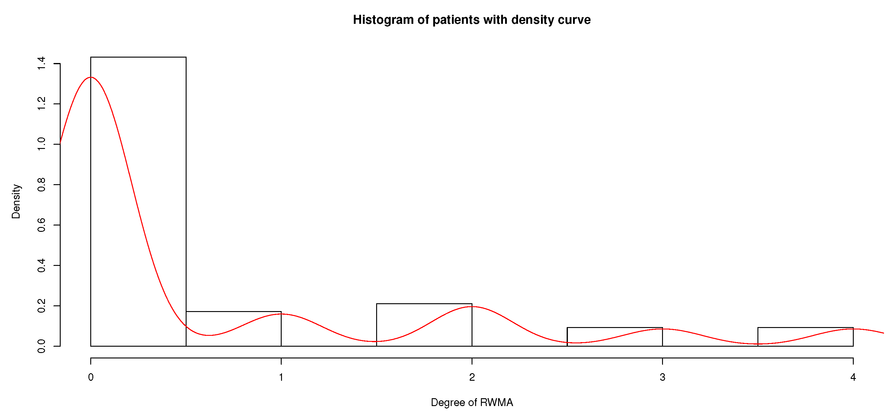
The data of heart disease were provided by UCI Machine Learning Repository [26]. There are 303 patients present in the underlying data set (Cleveland, Hungary, Switzerland, and the VA Long Beach, on 1 July, 1988). The summary statistics on the number of people affected by RWMA such as mean (0.62) and variance (1.28) are different, and the degree of abnormalities of regional wall motion (i.e., normal, mild, moderate, severe, and extreme) are also considered in this work. This provides an evidence of over-dispersion in the counts.

The histogram in Figure 1 depicts a skew distribution with over 72% of zero counts. The two phenomena over-dispersion and zero inflation exhibited by the data need to be accounted for by our model. The over-dispersion is present and has an excess of zero counts in the underlying data set, so we have to consider zero inflated regression models. Simultaneously, since both are present here, we demonstrate (i) the zero inflated Poisson (ZIP) and (ii) zero inflated negative binomial (ZINB) statistical models obviously in this work.

The control of risk factors of cardiovascular disease (CVD) is very difficult in reducing the risk of CVD in persons who already have diabetes. Recently, some clinical trials have demonstrated that the use of more aggressive targets for cholesterol and blood pressure control among individuals with diabetes results in reduced incidences of CVD events [27,28,29]. The individuals with diabetes had greater reductions in total and LDL cholesterol compared to those without diabetes and similarly declined in cases with high blood pressure levels. Improvements in the case of such risk factor levels is paralleled by increasing the number of different treatments with drugs. Diabetes mellitus is highly related to an overall two- to three-fold increased risk of mortality due to CVD [30,31,32]. Generally, the maximum likelihood estimation (MLE) method is used to obtain the parameters estimation in such models.

3.1. Model Fitting with Bayesian Approach (For No Covariates)

First, we utilized the data set in the absence of explanatory variables. Moreover, regular Negative Binomial and Poisson distributions were fitted to the underlying data set for a comparison with the zero-inflated models. We used the software WinBUGS to generate samples from the posterior distribution of the parameters. After generating samples from the posterior distribution, the parameters $p,\theta$; zero defect probability ⇔ P(Y = 0); and the deviance were observed to evaluate the convergence of the Markov Chain Monte Carlo (MCMC) method. Deviance is a measurement of goodness-of-fit for a statistical model and is basically used in hypothesis testing. e.g., in the case with no covariate, deviance is defined such as deviance ≡ $-2log\left[L\right\{(p,\theta )\left|Y\right\}].$ Since in this situation deviance is only a function of the parameters, the posterior distribution of deviance is simply derived from the MCMC iterations using WinBUGS software. In this work, Bayesian zero inflated regression models without and with covariates are also involved. For each Bayesian estimation run, we applied Gibbs sampling with 10,000 MCMC iterations and three chains to the zero inflated models by using the WinBUGS based on the diagnostic results. For the no covariate case, we started with the assumption of a uniform prior over $(0,1)$ with the p parameter and a gamma prior over $(0.5,0.5)$ with the $\theta$ parameter.

For negative binomial models, the posterior means of the deviance are about $241.87$, and for Poisson models, it is about $244.92$. Therefore, it indicates that negative binomial models have roughly better performance than Poisson models. However, $P(Y=0)$ from the zero inflated Poisson regression model, estimated by posterior mean and median, are very closer to the empirical estimates of zero counts (0.72 in our data), which suggests a better fit to the ZIP model when compared with negative binomial or Poisson distributions and Bayesian estimations to obtain such information.

3.2. Simulation Studies for Comparison

Now, to show a validation of the Bayesian method, we evaluate the ZIP model (with appropriate statistics) without covariates for a better understanding of this model. Here, three simulation studies based on the ZIP model are presented. In the simulation for study-1, $p=0.1$, $\theta =1$, and $P(Y=0)=0.43$; in the simulation for study-2, $p=0.5$, $\theta =1$, and $P(Y=0)=0.68$; and similarly in the simulation for study-3, $p=0.9$, $\theta =1$, and $P(Y=0)=0.94$ are used. For each case, sample size is considered 100 and is repeated 10,000 times. The results are based on c.p.(coverage probabilities with $95\%$ interval estimates) in

Table 1. Simulation for c.p. based on $95\%$ C.I. and RMSE.

Study	Parameter/Quantity	Classical Method					Bayesian Method					% Average Reduction in ALCI
		Std. dev	CI	CP	ALCI	RMSE	Std. dev	CI	CP	ALCI	RMSE
Study I	$p=0.1$	0.023	(0.233, 0.789)	0.928	0.56	0.803	0.0733	(0.302, 0.874)	0.944	0.57	0.801	86%
	$\theta =1$	0.0302	(0.010, 0.887)	0.942	0.88	0.052	0.201	(0.019, 0.879)	0.958	0.86	0.051
	$P\left(Y=0\right)=0.43$	0.0643	(0.019, 0.984)	0.902	0.98	0.006	0.001	(0.201, 0.741)	0.52	0.55	0.005
Study II	$p=0.5$	0.2827	(0.301, 0.792)	0.962	0.49	0.403	0.0535	(0.286, 0.839)	0.952	0.55	0.406	24%
	$\theta =1$	0.107	(0.112, 0.805)	0.931	0.69	0.071	0.023	(0.080, 0.901)	0.943	0.82	0.072
	$P\left(Y=0\right)=0.68$	0.033	(0.011, 0.787)	0.97	0.78	0.019	0.0042	(0.049, 0.682)	0.91	0.63	0.016
Study III	$p=0.9$	0.2062	(0.333, 0.822)	0.954	0.49	0.015	0.0553	(0.341, 0.789)	0.938	0.45	0.016	35%
	$\theta =1$	0.643	(0.182, 0.769)	0.924	0.59	0.154	0.204	(0.201, 0.755)	0.946	0.55	0.155
	$P\left(Y=0\right)=0.94$	0.032	(0.008, 0.984)	0.982	0.98	0.043	0.035	(0.101, 0.837)	0.986	0.74	0.031

. The classical $95\%$ confidence intervals are derived by turning around the LRT (likelihood ratio tests) based on chi-square distribution with a large sample. The frequency and Bayesian estimates of each of the parameters $\theta$ and p are very close (but in Study-3, the estimation of $\theta$ is different), and these suggests that the performance of the Bayesian approach is better to estimate $P(Y=0)$ (see Table 1). For example, the average length reduction in the intervals are $86\%$ and $35\%$ in the cases of study-1 and study-3, respectively. It is concluded (from Table 1) that the intervals in the case of the Bayesian method are very competitive for c.p. (coverage probabilities). It also provides that the width of the Bayesian intervals are significantly shorter than MLE when $P(Y=0)$ is very close to one. For each case (study-1, -2, and -3), the sample size is considered 50, and proceeding in the similar manner, we get the results (based on c.p.) for study-1: 0.724, 0.853, and 0.822, respectively (for classical), and 0.969, 0.943, and 0.901, respectively (for Bayesian); for study-2: 0.892, 0,919, and 0.890, respectively (for classical), and 0.923, 0.911, and 0.853, respectively (for Bayesian); and similarly, for study-3: 0.874, 0.853, and 0.822, respectively (for classical) and 0.917, 0.889, and 0.867 (for Bayesian), respectively. Therefore, as per the simulations, the Bayesian method (specially for study-1 and study-3) obtains a higher probability of convergence than the classical method. Next, for comparison, the root mean square error (RMSE) was also evaluated in terms of classical and Bayesian estimations.

In study-1, the RMSE and standard deviation (std.dev.) of the estimates based on MLE are $0.803$ (std.dev. = $0.023$), $0.052$ (std.dev. = $0.0302$), and $0.006$ (std.dev. = $0.0643$) for $p,\theta$, and P (Y = 0), respectively, whereas the corresponding RMSE and standard deviation in the case of Bayesian estimation are $0.801$ (std.dev. = $0.0733$), $0.051$ (std.dev. = $0.201$), and $0.005$ (std.dev. = $0.001$) for $p,\theta$, and P(Y = 0), respectively. From study-2, the RMSE and standard deviation of the MLE are $0.403$ (std.dev. = $0.2827$), $0.071$ (std.dev. = $0.107$), and $0.019$ (std.dev. = 0.033) and the RMSE and standard deviation of the Bayesian estimates were 0.406 (std.dev. = 0.0535), 0.072 (std.dev. = 0.023), and 0.016 (std.dev. = 0.0042) for the parameters $p,\theta$, and $P(Y=0)$, respectively. Lastly, in study-3, the RMSE and standard deviation of the MLE estimates are 0.015 (std.dev. = 0.2062), 0.154 (std.dev. = 0.643), and 0.043 (std.dev. = 0.032) and the corresponding Bayesian estimates are 0.016 (std.dev. = 0.0553), 0.155 (std.dev. = 0.204), and 0.031 (std.dev. = 0.035) for the parameters $p,\theta$, and $P(Y=0)$ respectively.

In a similar manner, we can obtain the results for study-1: 0.801, 0.168, and 0.159, respectively (for classical), and 0.772, 0.141, and 0.143, respectively (for Bayesian); for study-2: 0.356, 0.321, and 0.280, respectively (for classical), and 0.369, 0.301, and 0.299, respectively (for Bayesian); and similarly, for study-3: 0.240, 0.501, and 0.272, respectively (for classical), and 0.147, 0.442, and 0.258 (for Bayesian), respectively, for the small sample (i.e., n = 50). When the sample size is large, the RMSE from are also quite similar for the two methods. However, it is shown by the simulations that the Bayes estimator also has a smaller RMSE value than MLE in the case of a small sample (in this work, we used $n=50$ and $p=0.1$ or $p=0.9$). The results from the simulation results provide that the Bayesian approach gives a better performance than the MLE for smaller RMSE and larger c.p. when samples sizes are small along with either very low or very high cases of zero inflated counts.

Our simulation studies indicate that the Bayesian approach provides better performance because it yields smaller bias and larger coverage probabilities than the classical maximum likelihood method, particularly when the sample sizes are small with very low or very high cases of zero inflated counts. When n is sufficiently large, MLE and Bayesian both perform well and the difference between the two approaches are almost identical (for this reason, we get almost the same RMSE in both cases). Therefore, the MLEs and the Bayesian estimates act very indistinguishable and both have an identical asymptotic normal distribution (when n is very large).

3.3. Simulation Studies in Presence of Covariates (Using Bayesian Approach)

For regression cases, the normal distribution is assumed prior for the regression parameters $\alpha$ and $\beta$. In particular, for the assumption of normal distribution, we considered the mean to be 0 with a very large variance, 1000. A reasonable choice of initial values for $\alpha$ and $\beta$ in the MCMC method can be prevailed by fitting the underlying models using statistical software [24]. In

Table 2. Posterior summary of parameters (with covariates): ZIP model.

Model	Parameter	Predictors	Mean	Sd	Percentile			ALCI
					25%	50%	97.5%
ZIP$\left(p,\theta )\right)$	p	Intercept	11.456	2.34	3.053	11.289	19.496
		Age	0.192	0.008	0.017	0.184	12.194	12.2
		Obesity	0.234	0.184	−1.002	0.198	22.279	23.3
		Weight	0.112	0.029	−0.142	0.117	15.122	15.2
		BMI	0.027	0.083	−2.132	0.017	19.024	21.5
		Sex	−0.7	0.532	3.456	−0.865	10.701	14.1
		HBP	−0.005	0.01	−5.019	−0.098	11.13	16.1
		PR	−0.024	0.017	−1.724	−0.127	8.924	10.6
		PTS	1.22	1.07	0.001	0.034	21.28	21.2
		ETS	−0.407	0.45	−4.432	−0.977	17.412	21.8
		DM	−0.768	0.521	−6.768	−1.597	9.768	15.5
		HT	−0.119	0.428	−3.113	−0.154	8.169	11.2
		CRF	1.209	1.32	0.034	1.201	18.209	18.2
		Dylipidemia	0.392	0.351	−0.092	0.192	21.392	22.4
		WPP	0.707	1.399	−0.049	0.678	17.997	18.0
		LR	−0.855	1.031	−3.899	−0.987	13.855	17.7
		TCP	−0.761	0.355	−3.989	−0.861	21.761	24.6
		Dyspnea	0.392	0.351	−2.398	0.378	22.392	24.6
		Q−wave	−1.27	0.826	−4.297	−1.23	9.279	13.5
		LVH	1.212	0.75	0.002	1.103	19.212	19.2
		FBS	0.004	0.004	−2.004	0.001	8.654	10.6
		Creatine	0.224	0.664	−3.334	0.225	18.984	21.4
		Trygyceride	−0.005	0.003	−4.875	−0.012	8.005	12.9
		LLPD	0.007	0.005	−3.543	0.005	12.345	15.8
		HLPD	0.005	0.017	−2.329	0.005	11.987	13.3
	$\theta$	Intercept	−2.393	0.098	−4.987	−2.389	−0.879
		Age	2.57	0.002	0.985	2.55	1.939	0.95
		Obesity	0.556	0.104	0.234	0.508	2.279	1.9
		Weight	1.179	0.012	0.166	1.173	5.767	5.6
		BMI	1.132	0.033	0.182	1.132	3.398	3.2
		Sex	0.076	0.421	−0.019	0.065	2.991	0.07
		HBP	−0.002	0.009	−0.419	−0.002	3.751	4.1
		PR	1.693	0.012	0.677	−0.112	6.924	6.2
		PTS	0.192	0.938	−0.042	0.032	7.28	7.3
		ETS	−0.449	0.333	−2.121	−0.897	5.401	7.5
		DM	0.188	0.334	−1.178	−1.566	3.768	4.9
		HT	0.076	0.428	−2.006	−0.154	8.169	6.1
		CRF	0.062	1.292	−3.061	1.234	7.75	10.8
		Dylipidemia	0.607	0.281	−2.637	0.159	5.598	8.2
		WPP	−1.355	1.01	−3.336	0.787	4.998	7.3
		LR	−2.461	1.017	−5.437	−0.987	4.574	1.0
		TCP	0.892	0.223	−2.972	−0.909	4.912	6.8
		Dyspnea	−1.266	0.351	−3.284	0.895	8.354	11.6
		Q−wave	2.931	0.546	0.274	−1.242	8.75	8.5
		LVH	0.104	0.497	−1.892	0.103	8.643	9.5
		FBS	0.233	0.004	2.277	0.23	7.25	4.9
		Creatine	−1.005	0.562	−4.937	0.195	5.565	9.5
		Trygyceride	0.005	0.003	−2.744	0.005	7.586	10.1
		LLPD	0.031	0.002	−1.771	0.029	3.999	5.6
		HLPD	0.762	0.009	−2.712	0.654	3.909	6.7
	Sample Mean $P\left(Y=0\right)$		0.728	0.078	0.093	0.73	0.899	0.8
	Deviance		216.93	15.701	201.54	216.87	220.91	18.7

, a posterior summary for the zero inflated model is presented. For the parameters, $2.5\%$ and $97.5\%$ contribute an equal tail in the case of $95\%$ posterior interval estimation. Additionally, we demonstrated data on covariates that might clarify the variation in the zero counts. The regression models that are used in the case of discrete distributions (i.e., Poisson and Negative Binomial) may not have a good fit on the underlying data set, and it underestimate the zero counts probability [19], which is of utmost importance in the case of heart disease. The covariates are linked with model parameters p and $\theta$ in a ZIP regression [21]. A model having a little more refined algorithm such as data augmentation is needed when covariates are present.

In applied research, regression models are very useful for scrutinizing significant roles due to the effects of covariates and possess relationships between the responses and major predictors. In general, for the independently distributed responses, $Y_i$ sampled from ZIP ($p_i,{\theta }_i$) is used to link functions: (i) The covariates are related to p through a logit model, and (ii) the covariates are related to $\theta$ through a log-linear model.

The zero inflated models were fitted to the count data of the mentioned covariates. In the previous section, WinBUGS was used for fitting both regressions and similar convergence diagnostics are used here, which were already described in a previous section. Next, a summary (mean, std.dev., $2.5\%$, median, and $97.5\%$) of the parameters from zero inflated models are presented in Table 2. A positive intercept in Table 2 of $11.456$ with a $95\%$ posterior interval [0.386, 40.643] points out that the possibility of being in the zero state is very high; moreover, the sample mean of the zero defect probability is 0.728 (which is very close to the empirical percentage of zero counts) with the $95\%$ posterior interval [0.683, 0.752], but in the case of the ZINB model, it does not happen (since the sample mean of the zero count probability is 0.746). Apart from this, for the ZINB model, our simulation studies indicate that the deviance changes slightly to 234.87 from the deviance mentioned in

Table 3. Posterior summary (without covariates): zero inflated models.

Model	Parameter/Quantity	Mean	Sd	Percentile			Average Length of CI
				25%	50%	97.5%
ZIP$\left(p,\theta )\right)$	$\theta$	0.432	0.064	0.231	0.433	0.675	0.44
	p	0.786	0.354	0.322	0.792	0.893	0.57
	$\mu =(1-p)\theta$	0.558	0.267	0.145	0.556	0.764	0.62
	$P\left(Y=0\right)$	0.722	0.087	0.083	0.721	0.873	0.79
	Deviance	244.97	15.7	216.38	216.87	220.91	4.51
ZINB$\left(p,\theta ,r)\right)$	$1-\theta$	0.862	0.08	0.674	0.884	0.937	0.26
	r	4.12	2.43	3.389	3.87	8.989	5.6
	p	0.782	0.42	0.252	0.84	0.764	0.51
	$\mu =r(1-p)\frac{\theta }{1-\theta }$	0.562	0.344	0.342	0.561	0.734	0.39
	$P\left(Y=0\right)$	0.739	0.77	0.643	0.731	0.872	0.23
	Deviance	241.87	19.7	213.33	215.78	217.7	4.40

, but it is shown in Table 2 that the deviance is dropped by a lot to 216.93 from the deviance in Table 3 for the case of the ZIP model. In the underlying model (ZIP), there may be a number of groups with a different number of parameters related to heart disease. The numerical results of the parameter estimation of the model clearly demonstrate the efficacy of the proposed approach. With the reference being males, we observe a negative coefficient $-0.679$ with p-value $0.02$ for females (shown in Table 2). The decrement is represented by a percentage of $49.29\%$, so the results provide that the probability of heart disease counts is reduced for females compared with males. Here, it is also mentioned that there is a myth that coronary artery disease (CAD) is less common and less severe in women. However, in our work, although men are more affected than women, heart disease due to CAD is not negligible in the case of women. A 50-year-old woman’s risk of dying from CAD is 10 times more than her mortality risk from hip fracture and breast cancer combined. Although mortality from ischemic heart disease (IHD) has declined, as per our observations, it is of a lesser magnitude in women compared with men of a similar age [33]. It is also obtained from Table 2 that the estimated coefficient of $0.5158$ (for obesity) is highly significant ($p<0.01$); we deduce that the increasing effect of obesity on the expected number of CAD affected persons is about $67.50\%$ as there is a positive association between obesity and cholesterol level [34]. Diabetes mellitus (DM) is one of the highest risk factors for heart disease. In our work, it is observed that persons with diabetes mellitus are affected more by heart disease (CAD). Among adults (with DM), there is a prevalence of 70–80% for elevated low density lipoprotein (LDL), of 60–70% for obesity, and of 75–85% for hypertension [35]. Diabetes mellitus (DM) is associated with increased mortality risk of heart disease. More than $70\%$ of people older than 65 years with diabetes mellitus die from heart disease or stroke [36]. Similarly, it is observed that current smokers are at more than $20\%$ more risk of CAD than ex-smokers. Typical chest pain is of an important risk factor in our studies. The increment in typical chest pain of a person is affected more in regional wall motion abnormalities. Moreover, some secondary factors (i.e., creatine, dyslipidemia, congestive heart failure, Q-wave, etc.) have strong influences on heart disease.

4. Concluding Remarks

In this work, we have analyzed the effects of the most significant predictors that could explain the risk of having CAD or dying from myocardial infarction, for instance. We have obtained the significance of modelling for excess zero in count data structure in the context of the Bayesian method. The Bayesian method has a better small sample performance than the classical method with tighter interval estimates and better coverage probabilities. It can also be concluded that the Bayesian approach provides better performance than the classical maximum likelihood estimation in the sense of yielding larger coverage probabilities and smaller root mean square error. Moreover, in this work, we have analyzed the effect of risk factors that could explain the number of victims of heart disease and obtained fruitful conclusions from the interpretations of the results related to heart disease. This analysis evidently endorses the perception of people concerning heart disease. The major risk factors for coronary heart disease are obesity, diabetes mellitus, cholesterol, smoking, etc. Apart from these, some secondary risk factors are also influenced by heart failure. Being female also reduces the risk of fatality compared with being male but the risk in females due to CAD is not imperceptible. In a previous, work it was only demonstrated by assessing the importance of cardiovascular risk factors with various approaches [37]. However, in this work, we not only analyze the effect of risk factors but also perform the Bayesian approach. Moreover, it is shown that the Bayesian method has a better small sample performance than the classical method, which was not performed in an earlier work [24]. It was shown earlier that, if negative binomial is better than Poisson (for the excess zero count data set), then ZINB is better than ZIP [38]. However, in our work, we have shown that the ZIP model is best among all, although Poisson is the worst among all.

Zero inflated models have been utilized to manage such count data, and are estimated conventionally using maximum likelihood estimator. Apart from this, Bayesian methods have been utilized for estimating ZIP model because these methods provide various advantages in comparisons with the maximum likelihood estimation for this model. In this context, it is mentioned that Bayesian intervals (also known as credible intervals) give a strong impetus for adopting the perspective of the Bayesian analysis. It is very influential (basically in the case of the ZIP model) that the Bayesian approach can provide full joint distribution of the parameters (in which we are interested). It can account for different sources of uncertainty in the case of the zero inflated model with count data that is not easy to achieve in traditional maximum likelihood methods [39]. The zero inflated model has the following advantages: (i) it is very useful for modeling the outcomes of regional wall motion abnormalities due to CAD and various situations where count data have excess zeros, and (ii) it is also very useful for process optimization in the presence of covariates. In this work, the Bayesian analysis was used to model such types of count data (with excess zeros) by using sampling-based techniques. It can be also concluded from simulations that the proposed method is very effective for inferences when the sizes of samples are small. We also performed simulations based on small sample (such as $n=25,50$ etc.) which depicts that the proposed approach provides a better performance in the case of a small sample than the classical method [39] with interval width and better coverage probabilities (from Table 2 and Table 3). The collinearity problem has emerged due to the strong impact between some covariates such as obesity, weight, and BMI (body mass index). However, in the present work, we avoid such effects [40,41].

Since the data have lots of zero, between Poisson and negative binomial models, sometimes Poisson gives better results than negative binomial and sometimes negative binomial gives better results after the data are fitted to the model. If negative binomial gives better results than Poisson, then generally, it was shown that zero inflated negative binomial is the best model among Poisson, negative binomial, zero inflated Poisson, and zero inflated negative binomial for excess zeros data [38]. On the other hand, if Poisson gives better than negative binomial, then the zero inflated Poisson model is the best model among all (i.e., Poisson, negative binomial, zero inflated Poisson, and zero inflated negative binomial) for excess zero data [24,42]. However, in this work, the Poisson model is the worst among all despite the zero-inflated Poisson model (ZIP) being the best fitted among the models (considered here), which has been verified with various procedures.

The usefulness of zero inflated models (ZIP, ZINB, etc.) are displayed in the current work, where count data with excess zeros are encountered. Although the ZIP model is used with the Bayesian approach and utilizes the significant role of the covariates, sometimes, the models give biased parameters due to over-dispersion. Apart from this, the interactions between available covariates is not contemplated in much research.

References

- World Health Organization. 2019. Available online: https://www.who.int/news-room/fact-sheets/detail/the-top-10-causes-of-death (accessed on 9 December 2020).
- Centers for Disease Control and Prevention. 2009. Available online: HeartDiseaseFactscdc.gov (accessed on 15 July 2009).
- Roth, G.A.; Johnson, C.; Abajobi, A. Global, Regional, and National Burden of Cardiovascular Diseases for 10 Causes, 1990 to 2015. J. Am. Coll. Cardiol. 2017, 70, 1–25. [Google Scholar] [CrossRef] [PubMed]
- Diamond, G.A.; Forrester, J.S. Analysis of probability as an aid in the clinical diagnosis of coronary-artery disease. N. Engl. J. Med. 1979, 300, 1350–1358. [Google Scholar] [CrossRef] [PubMed]
- Pryor, D.B.; Harrell, F.E., Jr.; Lee, K.L.; Califf, R.M.; Rosati, R.A. Estimating the likelihood of significant coronary artery disease. Am. J. Med. 1983, 75, 771–780. [Google Scholar] [CrossRef]
- National Institute for Health and Clinical Excellence (NICE). Chest Pain of Recent Onset: Assessment and Diagnosis; CG95: London, UK, 2018; Available online: https://www.nice.org.uk/guidance/cg95 (accessed on 5 April 2018).
- He, T.; Liu, X.; Xu, N.; Li, Y.; Wu, Q.; Liu, M.; Yuan, H. Diagnostic Models of the Pre-Test Probability of Stable Coronary Artery Disease: A Systematic Review, Clinics. 2016. Available online: https://pdfs.semanticscholar.org/9092/72539b4b6ce37c4821abd3f1eef5ad4ae091.pdf (accessed on 16 December 2016).
- 2019 European Society of Cardiology. 2020. Available online: https://www.escardio.org/Guidelines/Clinical-Practice-Guidelines/Chronic-Coronary-Syndromes (accessed on 14 January 2020).
- American Family Physician. AHA/ACC/ASH Release Guideline on the Treatment of Hypertension and CAD. 2015, 92, pp. 1023–1030. Available online: https://www.aafp.org/afp/2015/1201/p1023.html (accessed on 1 December 2015).
- Montalescot, G.; Sechtem, U.; Achenbach, S. ESC guidelines on the management of stable coronary artery disease: The Task Force on the management of stable coronary artery disease of the European Society of Cardiology. Eur. Hear. J. 2013, 34, 2949–3003. [Google Scholar]
- Fihn, S.D.; Gardin, J.M.; Abrams, J. ACCF/AHA/ACP/AATS/PCNA/SCAI/STS Guideline for the Diagnosis and Management of Patients With Stable Ischemic Heart Disease: Executive Summary: A Report of the American College of Cardiology Foundation/American Heart Association Task Force on Practice. J. Am. Coll. Cardiol. 2012, 60, 2564–2603. [Google Scholar] [CrossRef] [Green Version]
- Safford, R.E.; Bove, A.A. Prediction of coronary artery disease by left ventricular regional wall motion abnormalities in patients with stenosis ofthe aortic valve. Br. Heart J. 1987, 57, 237–241. [Google Scholar] [CrossRef] [Green Version]
- Alizadehsania, R.; Habibi, J.; Hosseini, M.J.; Mashayekhi, H.; Boghrati, R.; Ghandeharioun, A.; Bahadorian, B.; Sani, Z.A. A data mining approach for diagnosis of coronary artery disease. Comput. Methods Programs Biomed. 2013, 111, 52–61. [Google Scholar] [CrossRef]
- Karaolis, M.A.; Moutiris, J.A.; Hadjipanayi, D. Assessment of the Risk Factors of Coronary Heart Events Based on Data Mining with Decision Trees. IEEE Trans. Inf. Technol. Biomed. 2010, 14, 559–566. [Google Scholar] [CrossRef]
- Agresti, A. An Introduction to Categorical Data Analysis; John Wiley and Sons: New York, NY, USA, 2002. [Google Scholar]
- Ghosh, S.; Samanta, G.P. Statistical modelling for cancer mortality, Letters in Biomathematics. 2019, Volume 6. No. 2. Available online: http://0-dx-doi-org.brum.beds.ac.uk/10.1080/23737867.2019.1581104 (accessed on 2 March 2019).
- Shankar, V.; Milton, J.; Mannering, F. Modelling Accident Frequencies as Zero-Altered Probability Processes: An Empirical Inquiry. Accid. Anal. Prev. 1997, 29, 829–837. [Google Scholar] [CrossRef]
- Spiegelhalter, D.; Lunn, J.; Thomas, A.; Best, N. WinBUGS—A Bayesian modelling framework: Concepts, structure, and extensibility. Stat. Comput. 2000, 10, 325–337. [Google Scholar]
- Miaou, P. The relationship between truck accidents and geometric design of road sections: Poisson versus negative binomial regressions. Accid. Anal. Prev. 1994, 26, 471–482. [Google Scholar] [CrossRef] [Green Version]
- Mullahy, J. Specification and testing of some modified count data models. J. Econom. 1986, 33, 341–365. [Google Scholar] [CrossRef]
- Lambert, D. Zero-Inflated Poisson Regression, with an Application to Defects in Manufacturing. Technometrics 1992, 34, 1–14. [Google Scholar] [CrossRef]
- Czado, C.; Erhardt, V.; Min, A.; Wagner, S. Zero-inflated generalized Poisson models with regression effects on the mean, dispersion and zero-inflation level applied to patent outsourcing rates. Stat. Model. 2007, 7, 125–153. [Google Scholar] [CrossRef] [Green Version]
- Wang, Z.; Shuangge, M.; Wang, C.Y. Variable selection for zero-inflated and overdispersed data with application to health care demand in Germany. Biom. J. 2015, 57, 867–884. [Google Scholar] [CrossRef] [PubMed] [Green Version]
- Ghosh, S.K.; Mukhopadhyay, P.; Lu, J.C. Bayesian analysis of zero-inflated regression models. J. Stat. Plan. Inference 2006, 136, 1360–1375. [Google Scholar] [CrossRef]
- Gelfand, A.E.; Smith, F.M. Sampling-Based Approaches to Calculating Marginal Densities. J. Am. Stat. Assoc. 1990, 85, 398–409. [Google Scholar] [CrossRef]
- UCI Machine Learning. 1988. Available online: https://archive.ics.uci.edu/ (accessed on 1 July 1988).
- Shepherd, J.; Barter, P.; Carmena, R.; Deedwania, P.; Fruchart, J.C.; Haffner, S.; Hsia, J.; Breazna, A.; LaRosa, J.; Grundy, S.; et al. Effect of lowering LDL cholesterol substantially below currently recommended levels in patients with coronary heart disease and diabetes: The Treating to New Targets (TNT) study. Diabetes Care 2006, 29, 1220–1226. [Google Scholar] [CrossRef] [Green Version]
- Hansson, L.; Zanchetti, A.; Carruthers, S.G.; Dahlof, B.; Elmfeldt, D.; Julius, S.; Menard, J.; Rahn, K.H.; Wedel, H.; Westerling, S. Effects of intensive blood-pressure lowering and low-dose aspirin in patients with hypertension: Principal results of the Hypertension Optimal Treatment (HOT) randomised trial. HOT Study Group. Lancet 1998, 351, 1755–1762. [Google Scholar] [CrossRef]
- Collins, R.; Armitage, J.; Parish, S.; Sleigh, P.; Peto, R. MRC/BHF Heart Protection Study of cholesterol-lowering with simvastatin in 5963 people with diabetes: A randomised placebo-controlled trial. Lancet 2003, 361, 2005–2016. [Google Scholar]
- Fox, C.S.; Coady, S.; Sorlie, P.D.; Levy, D.; Meigs, J.B.; D’Agostino, R.B.; Wilson, P.W.; Savage, P.J. Trends in cardiovascular complications of diabetes. JAMA 2004, 292, 2495–2499. [Google Scholar] [CrossRef] [Green Version]
- Gregg, E.W.; Gu, Q.; Cheng, Y.J.; Narayan, K.M.; Cowie, C.C. Mortality trends in men and women with diabetes, 1971 to 2000. Ann. Intern. Med. 2007, 147, 149–155. [Google Scholar] [CrossRef]
- Gu, K.; Cowie, C.C.; Harris, M.I. Diabetes and decline in heart disease mortality in US adults. JAMA 1999, 281, 1291–1297. [Google Scholar] [CrossRef] [PubMed]
- Heron, M.; Hoyert, D.L.; Murphy, S.L.; Xu, J.; Kochanek, K.D.; Tejada-Vera, B. Deaths: Preliminary data for 2006. Natl. Vital Stat. Rep. 2008, 56, 1–52. [Google Scholar]
- Veghari, G.; Sedaghat, M.; Joshghani, H.; Banihashem, S.; Moharloei, P.; Angizeh, A.; Tazik, E.; Moghaddami, A. Obesity and risk of hypercholesterolemia in Iranian northern adults. ARYA Atheroscler 2013, 9, 2–6. [Google Scholar]
- Preis, S.R.; Pencina, M.J.; Hwang, S.J.; D’Agostino, R.B., Sr.; Savage, P.J.; Levy, D.; Fox, C.S. Trends in cardiovascular disease risk factors in individuals with and without diabetes mellitus in the Framingham Heart Study. Circulation 2009, 12, 212–220. [Google Scholar] [CrossRef] [Green Version]
- Berry, C.; Tardif, J.C.; Bourassa, M.G. Coronary heart disease in patients with diabetes: Part II: Recent advances in coronary revascularization. J. Am. Coll. Cardiol. 2007, 49, 643–656. [Google Scholar] [CrossRef] [Green Version]
- Pencina, M.J.; Navar, A.M.; Wojdyla, D.; Sanchez, R.J.; Elassal, I.K.J.; D’Agostino, R.B.; Peterson, E.D.; Sniderman, A.D. Quantifying Importance of Major Risk Factors for Coronary Heart Disease. Circulation 2019, 139, 1603–1611. [Google Scholar] [CrossRef]
- Wiafe, E.S.; Kumi, A.A.; Nortey, E.N.N.; Idd, S. Modelling vehicular crash mortalities in Ghana. Model Assist. Stat. Appl. 2018, 13, 287–295. [Google Scholar] [CrossRef]
- Gelman, A.; Carlin, J.B.; Stern, H.S.; Rubin, D.B. Bayesian Data Analysis, 2nd ed.; Chapman and Hall/CRC: Boca Raton, FL, USA, 2004. [Google Scholar]
- Allison, P. When Can you Safely Ignore Multicollinearity? Stat. Horiz. Blog, 10 September 2012. Available online: http://statisticalhorizons.com/multicollinearity(accessed on 1 July 1988).
- O’Brien, R. Dropping highly collinear variables from a model: Why is it typically not a good idea? Soc. Sci. Q. 2016. [Google Scholar] [CrossRef]
- Neelon, B. Bayesian Zero-Inflated Negative Binomial Regression Based on Pólya-Gamma Mixtures. Bayesian Anal. 2018, 14, 829–855. [Google Scholar] [CrossRef]
Figure 1.
Frequencies of the degree of RWMA (from none to extreme).