
Dynamic Mixed Model Lotsizing and Scheduling for Flexible Machining Lines Using a Constructive Heuristic


1
School of Mechanical and Electrical Engineering, Guangzhou University, Guangzhou 510006, China
2
School of Mechanical Science and Engineering, Huazhong University of Science and Technology, Wuhan 430074, China
3
College of Mechanical and Electronic Engineering, Wenzhou University, Wenzhou 325035, China
4
Mechanical Engineering Department, The University of Lahore, Islamabad 45750, Pakistan
5
Department of Industrial Engineering, University of Engineering and Technology, Taxila 47080, Pakistan
*
Author to whom correspondence should be addressed.
Processes 2021, 9(7), 1255; https://0-doi-org.brum.beds.ac.uk/10.3390/pr9071255
Submission received: 18 June 2021
/
Revised: 12 July 2021
/
Accepted: 14 July 2021
/
Published: 20 July 2021
Abstract
:Dynamic lotsizing and scheduling on multiple lines to meet the customer due dates is significant in multi-line production environments. Therefore, this study investigates dynamic lotsizing and scheduling problems in multiple flexible machining lines considering mixed products. In addition, uncertainty in demand and machine failure is considered. A mathematical model is proposed for the considered problem with an aim to maximize the probability of completion of product models from different customer orders. A constructive heuristic method (CHLP) is proposed to solve the current problem. The proposed heuristic involves the steps to distribute different customer order demands among multiple lines and schedule them considering balancing of makespan between the lines. The performance of CHLP is measured with famous heuristics from the literature, based on the test problem instances. Results indicate that CHLP gives better results in terms of quality of results as compared to other famous literature heuristics.
1. Introduction
Manufacturers are striving to establish an effective and efficient production system, while facing changes in demand, fierce competition environments and uncontrollable production conditions. Based on the variety and volume of products, manufacturing industries use different kinds of production lines. In today’s manufacturing industry, flexible machining lines with automatic logistics equipment are the most preferred manufacturing system as they can produce a large number of customized products. Moreover, it is essential to regard manufacturing systems as cyber-physical systems (CPS) due to the development of networks and intelligent factories. CPS-based intelligent factories represent a form of future industrial network, while Industry 4.0 represents the concept of smart and intelligent manufacturing networks, that is, networks where machines, orders and products can interact without human control. The dynamic characteristics of a manufacturing system, such as product changes, demand fluctuation and the uncertainty of machine failure, pose challenges to the structure of manufacturing systems. This requires a dynamic manufacturing structure and scheduling scheme which can quickly respond to environmental changes, and this provides a good opportunity for the current research.
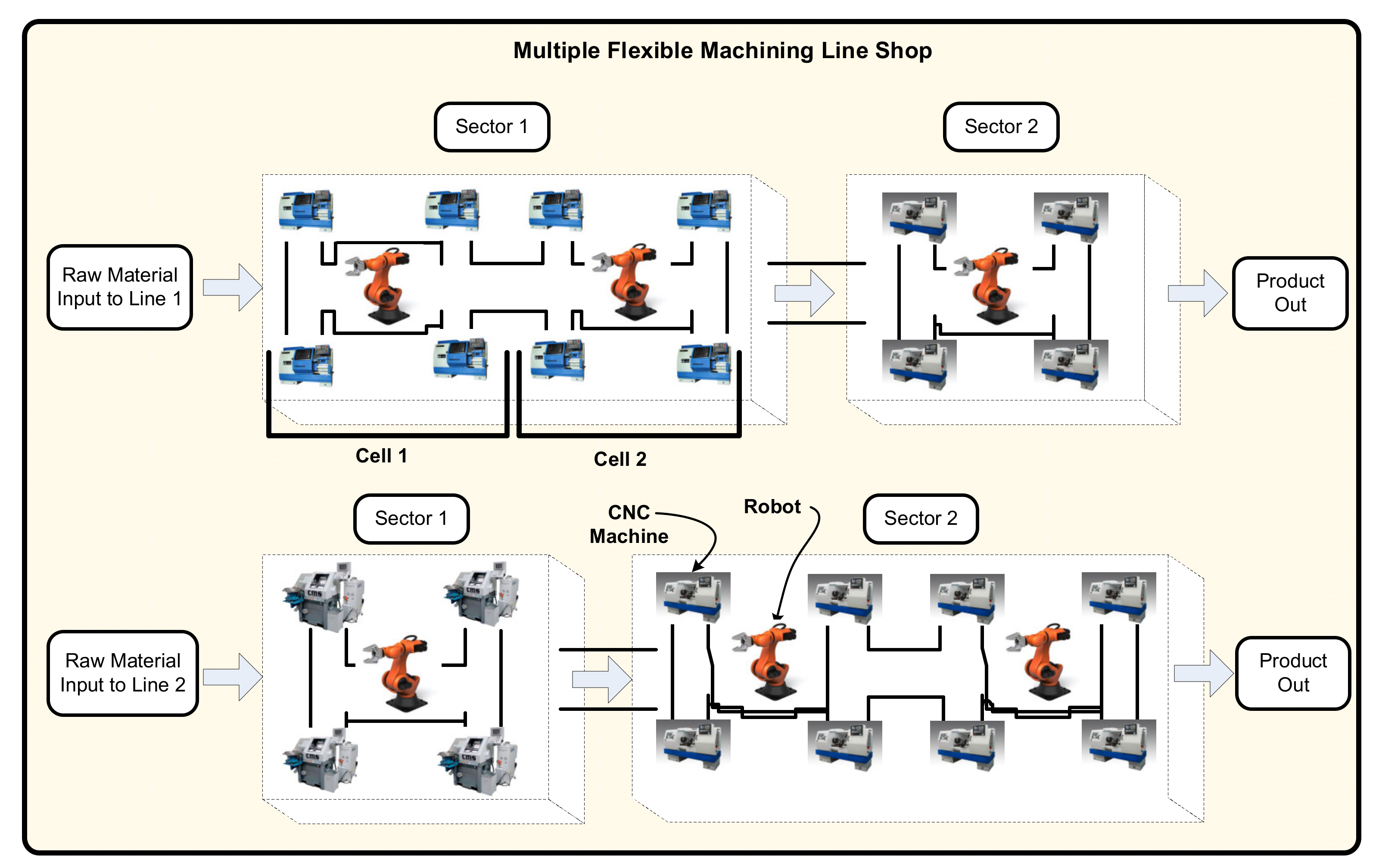
A Computer, Communication, Consumer (3C) flexible manufacturing system composed of multiple parallel flexible machining lines based on a real intelligent manufacturing project is considered here. Each flexible machining line has multiple machining sectors connected in series. Each sector is composed of multiple computerized numerical control (CNC) machines and various robots are used to transfer material to these machines in cells. In each cell, the machine can perform the same set of operations concurrently, which can raise the reliability of the system since the production line can still work during machine failures in most cases. There is an automatic conveyor in each line for transferring the parts between machining cells at a constant speed, which helps reduce the work-in-process. Each line has a different number of machines divided into sectors and therefore has different production capacities. The considered multiple flexible machining line shop is illustrated in Figure 1.
An optimal schedule of mixed models on these lines is critical to identify efficient production methods. Production in lots of mixed model products can reduce the setup time of equipment, improve productivity, and meet the in time needs of different customers. Therefore, in the actual industrial production scheduling level, it is practical to optimize the lotsizing and scheduling in different planning horizons. In the literature, lot sizing and scheduling in mixed model production systems has been addressed by several researchers. However, they mostly considered standard production system shop floor structures which are quite different and simple as compared to the flexible machining lines which are considered in the current research. In addition to the differences between production systems, there are additional complexities which are considered in the cur-rent research and make the current research novel. Lot sizing and mixed model scheduling in multiple parallel flexible machining lines were considered for the first time in theliterature by [1,2,3]. Further, due to practical importance in the industrial systems, this study considers lot sizing and scheduling in multiple lines in a dynamic environment by considering the demand of products as dynamically arriving with uncertain quantity. We consider uncertainty in machines and robot failure in the flexible machining lines for the first time in the literature. Reliability of the machines and robots is also taken into consideration while determining lot sizing and scheduling of lots on multiple lines. In addition, lot sizes of mixed models are created on multiple flexible machining lines by taking the load balance among multiple flexible machining lines into consideration.
The rest of the paper is organized as follows: Section 2 presents the related works in the literature. Section 3 presents the problem description. Section 4 illustrates the research methodology that includes the explanation of the proposed constructive heuristic for the lotsizing problem. Section 5 describes the computational experiments and results. Section 6 presents the conclusions and future directions of the research.
2. Literature Review
This section is divided into four different parts, each of which describes a related research review and the novelty of the current research accordingly. The current study addresses the problem of lot sizing and mixed model scheduling in flexible machining lines, therefore, the first part of this section presents a brief review of the literature related to production systems including transfer lines, machining lines, flexible machining lines and multiple flexible machining lines. The second part of research review is dedicated to the dynamic lot sizing and scheduling problem and this section explains the novelty of current research problem with respect to the dynamic lot sizing in multiple flexible matching lines. The third part of this section explains the literature related to the uncertain failure, reliability of machine and robots and its application in multiple flexible machining lines. The fourth part of the literature review explains the studies related to the optimization algorithms developed for lot sizing and mixed model sequencing. Further, it explains the novelty of current research with respect to the optimization method proposed in the current research.
2.1. Transfer Lines and Flexible Machining Line Problem
Dedicated machines in transfer lines can limit the flexibility of the machining processes and therefore, in recent advanced companies, transfer lines use CNC machines instead of dedicated machines to increase the flexibility in their processing operations. These lines are named flexible machining lines [4] and the balancing problem is called flexible machining line balancing problem (FMLBP) which is a major concern of modern manufacturing industries [4]. Liu [4] presented the line configuration and balancing problem for flexible machining lines to assign operations to the work stations, and determined the sequence of execution of operations which determined the number of machines required in each machining workstation to minimize the cycle time and number of machines in the line. Recently, the flexible machining lines balancing problem has been investigated by [1,2,3]. The machining lines considered in that work have a different design unlike transfer lines. These flexible machining lines are considered in the current research for the first time to improve the production.
The FMLBPs of flexible machining lines are based on a manufacturing company in China, where the flexible machining line is composed of number of CNC machines which are adjacent to each other and some of these machines along the line are allocated to the to perform the same process on the product along the line. CNC machines are grouped with one robot to form a cell, where the robot is used to serve the machines assigned to its corresponding cell. The CNC machines and one robot form a cell in their research [2,3]. Moreover, one or more than one cells which are adjacent to each other combine to make up a sector. In [2,3] research problems, each sector performs one operation and flexible machining line in contains serially connected sectors to perform operations on products moving from one sector to the next. Having more than one machine in cells and more than one cell in each sector increases the product production rate. The automation in parts movement in the cell can reduce the waiting time and loading-unloading time. However, the flexible machining lines considered in the [2,3] articles are considered to produce a single type of product. Due to increased demand for and variety of products, mixed model flexible machining lines with a certain balanced configuration of machines on the lines is significant to make mixed model products. Mixed model production on flexible machining lines can make the basic flexible configuration and balancing problem complex. In recent competitive production environments, due to mass customization, there may be different demand for product models from several customers, each with their specific due dates. In this situation, it is hard to schedule the customer orders and their demand on flexible machining lines. Therefore, the current research is focused on the type of flexible machining lines which have been studied by He [2,3] and considered as mixed model production for the first time in the literature. The current research is focused on the scheduling of mixed model products on the considered flexible machining lines. In addition, due to the large requirement of production capacity, it is necessary that more than one flexible machining lines be working in parallel to meet the demand of customers in time which has not been investigated in the literature and therefore, is considered here for the first time.
2.2. Dynamic Lotsizing and Scheduling on Multiple Lines
In order to satisfy customer demands, mixed model production is mostly used to produce a variety of products in lots. In the production of lots it is a challenging task for manufacturing companies to achieve a better tradeoff between an acceptable production rate with setup time reduction and on-time delivery to customers. Therefore, lotsizing and mixed model sequencing problema have significant application in manufacturing industries. Lotsizing and scheduling problems have been well studied in the literature [5,6,7,8]. The literature, divides lotsizing problems into two categories, including single level systems and multi-level systems [9,10]. In single-level systems, the final product is produced from a single stage directly from a raw material, for example, products produced by forging, etc. [11], while in multi-level systems, the final products are produced in more than one stage. For example, raw material is processed in the first stage, later different components of the final product are made and assembled to form the final product in the next stages. In most manufacturing industries, products are made in multiple stages and therefore, the lotsizing and mixed model sequencing problem in a multi-stage production environment is the focus of the current study. In the literature, multi-level lotsizing problem have been studied by several researchers for different production environment [5,8,10,12,13,14,15]. Karimi [10] studied the multi-level lotsizing and scheduling problem in a job shop environment. Seeanner [14] studied lotsizing and scheduling in multi-level flow line production systems. Yue [8] studied the lotsizing and sequencing integrated optimization problem in mixed-model production systems. Masmoudi [13] studied lotsizing and scheduling problem models with energy consideration. Parveen and Akthar Hasin [11] and Sifaleras and Konstantaras [15] investigated mixed model lotsizing and scheduling problems for dynamic production systems.
In general, the literature has mostly focused on lotsizing problems for medium term planning horizons. However, in most real manufacturing companies, in order to satisfy the due dates given by the medium level plan, lotsizing and scheduling with optimal decisions must be made in short term planning periods. This short term planning period can be a day and depends on the cycle time of the products, but lotsizing and mixed model scheduling in multiple flexible machining lines has not been investigated to date and is therefore presented in the current research.
In addition, in most manufacturing companies, customer orders arrive dynamically with uncertain demand. Each customer order is composed of multiple products with different uncertain demands and due date. Due to the uncertainty of the newly coming orders, the companies usually need to urgently change the running schedule for the rush orders in each planning horizon. Moreover, the insertion of new demands of models may cause some lots to be completed later than their due dates. This dynamically changing pattern of lot sizes and schedule of the models from different orders on multiple flexible machining lines in each planning horizon is very practical. However, the lotsizing and scheduling problem in multiple flexible machining lines with uncertain demand for each short time horizon, has not been investigated in the literature and it is a novel aspect in the current research.
In addition, large volumes of product are produced in multiple production lines and limited literature has focused on the multiple line lotsizing and scheduling problem [16,17,18]. However, the production system considered in these studies are different from the flexible machining line considered in the current research. The current research is novel in considering the dynamic lotsizing and scheduling of mixed model product lots arriving dynamically from different customers with uncertain change in demands and due dates. Furthermore, lotsizing, the allocation of different lots to multiple flexible machining lines and scheduling of lots considering sequence-dependent setup times in different time horizons with continuous arrival of orders has not been studied in the literature, making the current research the first which considers dynamic lotsizing of models in multiple flexible machining lines.
2.3. Uncertainty in Machine and Robots Failure
In the literature, the balancing objective mostly considered is how to minimize the number of stations in the production line [19,20]. The design of lines haw been presented on the basis of the number of machines in the line which is concerned with the initial cost of the system. The least possible number of CNC machines involved can reduce the initial cost of the setup, however, in the design of automated flexible machining lines, the reliability of the system is more important as compared to the small increase of cost against the more reliable system because an uncertain failure of machines in the production line can cause more losses to companies. In most real manufacturing systems, smooth production is a very important concern. A failure in the system can stop the production and it is not advisable to repair the machines online while keeping the system idle. In the considered that in automated flexible machining lines, the CNC machines and robots may not always be reliable and there is always a possibility that they may fail for some time. Preventive maintenance for all the machines and robots is performed from time to time to avoid any uncertain failure due to unreliability of the equipment in the lines. This failure can increase the production time due to the repair time of the machines in the cells. The repair time will be different depending on the factor(s) which caused the failure in the machine or robot. The delay in production in a sector of flexible machining lines can cause a blockage. Limited research in the literature has considered the topic of uncertainty in flexible machining lines [1]. He [1] proposed scenario-based robustness criteria for multi-objective optimization in flexible machining lines. However, the lotsizing and scheduling problem in flexible machining lines considering uncertainty in the production system is considered for the first time here. Therefore, the current research is novel in considering the uncertain failure of CNC machines and robots in multiple flexible machining lines.
2.4. Solution Methodology
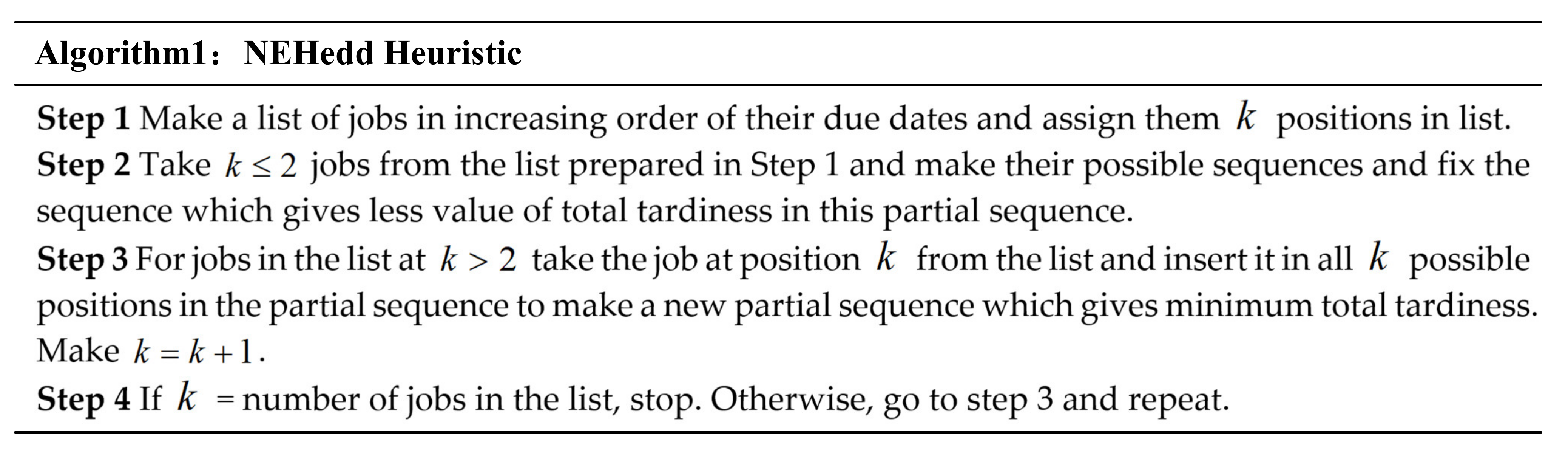
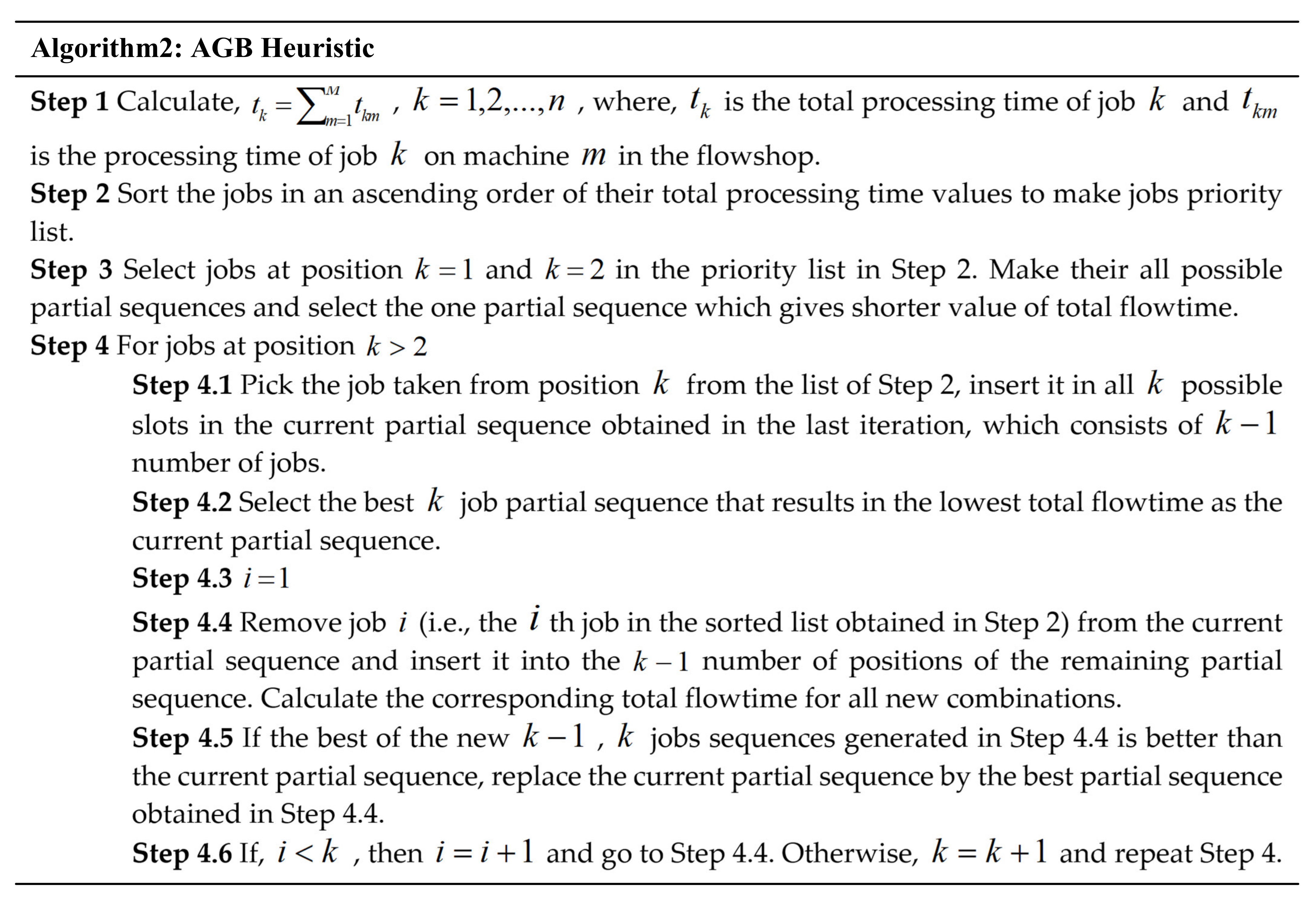
The scheduling problem of product lots in a machining line consisting of more than one machine is similar to the scheduling problem of jobs in flowshop [12,13,21,22,23]. The current problem of flexible machining lines containing different sectors is similar to a permutation flowshop. In the permutation flowshop problem, the most famous heuristic, proposed by Nawaz [24], is called the NEH (the abbreviation of Nawaz, Enscore and Ham) solution method. The NEH heuristic is an efficient constructive heuristic to minimize makespan [25] and it has been used by many researchers. The efficiency of NEH is due to its constructive steps in the partial sequence for setting jobs. The NEH heuristic has been improved by many researchers for their considered problems. For example, [26,27,28] extended the NEH heuristic to improve the performance of NEH for the objectives of makespan, idle time and total flow time. The partial sequencing of the NEH can limit its searching efficiency because after each job insertion, q partial sequence is made by insertion of only one job at different positions of the partial sequence. This idea can restrict the search for possible better local search solutions once a partial sequence is made. Framinan [24] used the same idea and performed pairwise exchanges of job sequences in the partial sequence after each iteration. Laha and Sarin [28] extended this idea and presented an extension of the NEH heuristic that performed job position exchanges in a partial sequence by checking all other possible slots in the partial sequence with an objective to minimize the total flow time. In [26,27,29] heuristics, the jobs are arranged in ascending order of the total processing time of jobs which is different from the NEH heuristic. This ascending order of jobs is used to make the partial sequences in these heuristics form a sequence which gives a smaller value of the total flowtime. Recently, Abedinnia [30] proposed a new constructive heuristic algorithm which is based on NEH and the algorithms proposed by [26] and [28] to minimize the total flow time in flowshop. In the flowshop problem, different criteria have been used to estimate the performance of the schedule. For example another extension of the NEH heuristic based on the due date of jobs has been developed in the literature by [28] who proposed a mechanism to develop the NEHedd method. The jobs are arranged according to earliest due date (EDD) rule to form a list and the jobs are taken from this list to make partial sequences to minimize the total tardiness of jobs. The current problem of lot scheduling on production lines is similar to the jobs scheduling problem in flowshop if each lot is considered as one job. A constructive heuristic is proposed in the current research for scheduling different lots on machining lines and modifying the allocation of different lots on different flexible machining lines. The proposed heuristic is inspired by the NEHedd heuristic and the heuristic proposed by [30]. The proposed heuristic method for the current problem is novel and introduced for the first time in the literature.
3. Problem Description
There are several customer orders each with demand of mixed model products with different due dates agreed by the company and customers. The customer orders are dynamically arriving and in each arrival, the demand of models and due date are uncertainly changing from the other demands in previous arrivals. There are different planning horizons and each horizon has a fixed number of days in it. The considered problem is focused on determining the production lot size of each model from each order in the planning horizon. Moreover, it is aimed to allocate these lots to different flexible machining lines and identify the mixed model sequence of the lots on each line in a planning horizon. These orders have possibility that some of the customer order demand may not be completed within the planning horizon and this demand is considered to be transferred and added in the next planning horizon. Furthermore, in each planning horizon, the newly arrived customer orders and uncompleted demand of previous planning horizon are collectively planned in the planning horizon. At first, in this section, the considered problem of lotsizing and scheduling on multiple lines is presented without taking into consideration the demand uncertainty and without machine and robot failure. Later, the model is presented with demand uncertainty and taking into consideration the machine failure or sector(s) failure.
3.1. Lotsizing and Scheduling with Known Demand
The demand of product models is considered as known in this section. The demand of product models is assigned to different production lines based on the cycle times of the lines. Each production line is considered to have different cycle time for different product models, if it is processed without processing other models on the line. Each line has an equal number of sectors but each sector has a different production rate in different lines. Therefore, for mixed model production in these multiple lines, we need to consider the cycle time of each line corresponding to each product model. The mixed model product lots are divided among the lines based on the cycle time. indicates the value of the sum of inverse of cycle time of all the lines for product models which is used to distribute the demand of product models among lines. The allowable demand of product models is indicated in Equation (1). Equation (2) indicates the allowable demand of product model from certain customer order. The number of product models for each product model which are assigned to the production line is illustrated in Equation (3). The initial lot size assigned to the production lines for each product model is indicated in Equation (4). The number of lots of each product model which are required to schedule in planning horizon is shown in Equation (5):
3.1.1. Completion Time of Models on First Sector
The processing time of the model which have not completed in the previous day and need to be completed in the current day and the sequence dependent setup time, if the uncompleted models of the previous day and the models which are to be processed in the current day are different.
Completion time of a model which is assigned at any position of a lot allocated at any position in lot sequence in first sector for day day in the planning horizon is given in Equation (6). The sequence dependent time indicated in Equation (7) shows the time, if there is a different model to process in the lot sequencing:
3.1.2. Completion Time of Models on Any Sector
Completion time of a model which is assigned at any position of a lot allocated at any position in lot sequence in any sector for day day is given in Equation (8). Completion time of a model which is assigned at first position of a lot allocated at any position in lot sequence in any sector for day day is given in Equation (9). Incomplete number of models from a lot of model m of order o on the line l in planning horizon is indicated in Equation (10). Available time left on production lines for a day in the planning horizon is shown in Equation (11). If , the model m will process on the day day in planning horizon .
3.2. Unreliable Machines in the Flexible Machining Lines
In the literature, the balancing objective that is mostly considered is how to minimize the number of stations in the production line [19,20]. The design of line has been presented on the basis of the number of machines in the line which is concerned with the initial cost of the system. A lesser number of stations or CNC machines can reduce the initial cost of the setup. However, in the design of automated flexible machining lines, the reliability of the system can be of more concern as compared to a small increase in the cost against the option of having a more reliable system because the delay in production due to uncertain failure of machines can cause more losses to the companies. Moreover, in real factories, there are many factors which can cause failures in machines or in the robots. These failures can increase the production time due to the repair time of the machines in the cells. The delay in production in a sector of flexible machining lines can cause a blockage or it can shift the bottleneck station and may lead to a change in the cycle time of the line. Therefore, the current research takes the failure of sectors into consideration during lotsizing and scheduling on parallel flexible machining lines.
3.2.1. Uncertain Failure of Machines and Robots
The reliability of machines and robots are very important for real manufacturing companies to ensure smooth production. Any blockage can increase the work in process inventory and make some sectors a bottleneck. The systems modeling without considering machine reliability is not very significant for companies. Therefore, in the current work, the reliability of machines and robots in the cells, sectors and the overall production line are considered. The reliability and availability of the CNC machines in the cells of different sectors depends on the repair rate and the failure rate of the machines. For an exponential distribution of machines failure and repair, the machine availability can be represented as given in Equation (12) [31] whereas the reliability of robots is given in Equation (13):
The proposed flexible machining line has more than one sector and each sector has one or more than one cells and each cell is composed of one robot and a certain number of machines. Therefore, the reliability equations for the cells, sectors and the overall line are presented here.
3.2.2. Reliability of a Cell
Each cell in the considered flexible machining line is composed of one robot and four CNC machines. These machines perform the same operation in a sector and work like parallel machines. If any machine has an expected failure, the other machines are not affected by this machine because they are in parallel to each other. The robot is connected to these machines in series and can affect the reliability of these machines if the robot is unavailable. Moreover, the cell cannot perform work if the robot is not available, or all the machines are not available. Therefore, the reliability of the cell can be presented as given in Equation (14):
3.2.3. Reliability of a Sector
In the considered flexible machining line, there are one or more than one cells which are connected in parallel to each other. Therefore, the reliability of the sector is can be computed from Equation (15):
3.3. Uncertainty in the Demand of models in Each Planning Horizon
In a real production environment, the demand of product models changes uncertainly due to several factors. For example, unexpected event occurs in market, uncertain change in season, an uncertain fall in the prices of competitors or uncertain change in the taxes or other pricing and demand-related factors can cause uncertain variations in the demand for products. Product demand uncertainty occurs due to several factors and each factor has its own probability to occur. The probability of occurrence of each factor and the change in the demand due to the corresponding factor are used to determine the uncertain proportion of the demand, as described in Equation (16). Each factor has its own probability of occurrence and each factor has its own influence on the demand of a product. Suppose that the change in demand due to each factor has a certain value from a uniform distribution of that factor i.e., , and each factor has a different range and there is a normal probability of each factor to occur, i.e., has normal trend to occur to change the demand . Then the demand can be normally distributed with uncertain mean value and variance , i.e., . Suppose the average demand of a product dependent on F number of independent factors, . is a binary variable. The mean value of the demand and variance value of demand are indicated in Equation (16) and Equation (19), respectively:
The average value of the demand which is required to schedule in the planning horizon is indicated in Equation (20). The demand of product models is considered as normally distributed and the demand of product models among the lines is distributed based on the cycle time of lines.
The average value of the allowable demand of product models which are assigned to the lines is indicated in Equation (21). The average value of product model from certain customer order which is allowed to process in a production line is indicated in Equation (22). The average value of the number of lots of product models from different orders which are assigned to a line in a planning horizon in indicated in Equation (23). The average value of the lot size of product model for a certain order on a production line in planning horizon in presented in Equation (24). The average value of the number of lots of product model from different order which are to schedule on the line in planning horizon is indicated in Equation (25):
The objective considered for the current problem is to minimize the models which cannot be produced before their respective due dates. In the current research, the orders are arriving dynamically and the demand of models is varying uncertainly. Therefore, the due date of the models may not have a constant value. It is assumed that the due date of the models in orders is normally distributed. Therefore, in different schedules on the lines, there is possibility that the models from different orders may get completed after their respective due date. Therefore, the objective to maximize the possibility to ensure that the models from different orders can get completed before their due date, is considered as an objective in the current research. The objective considering probability to ensure that the model from a certain order can be completed before its due date is given in Equation (26):
where, , and function . However, an exact solution for is difficult to obtain and therefore, Hayter, (1996) illustrated an approximation method to calculate which is shown in Equation (27). The objective can be computed from the simultaneous solution of the relations shown in Equations (27)–(29):
4. Research Methodology
The current scheduling problem of different product lots on the machining lines is similar to the job scheduling problem in a flowshop. Therefore, the heuristic algorithms proposed in the literature for flowshop problem that are used as inspiration for the proposed constructive heuristic for the lotsizing problem (CHLP) are illustrated in this section. These algorithms include the NEHedd heuristic [29] and the AGB (the abbreviation of Abedinnia, Glock and Brill) heuristic by Abedinnia [20]. NEHedd is mainly focused on the due date of jobs to give them priority while making the partial sequences and is used to reduce the total tardiness of jobs in a flowshop. It is similar with the NEH algorithm containing different priority-assigning criteria for jobs and different optimization objectives for flowshop scheduling, wheras AGB sorts jobs similar like NEH algorithm but it has additional steps of insertion of jobs in the partial sequences to improve the local search for job sequences. In addition AGB is significant to reduce the flowtime. Jobs scheduling or lot scheduling on a single line can utilize these algorithms effectively.
However, if these algorithms are used for lots scheduling on multiple lines, it may not be significant because each line may have different numbers of lots of products with different sizes of lots. Different lot sizes and different number of lots assigned to each line may create possibility that some production lines can complete the assigned lots earlier than the other production lines and the lines may not achieve a balanced workload. Therefore, it is desired to consider the balancing of workload during scheduling on multiple lines. In addition, the current problem involves uncertainty in demand and due date of customer orders. Therefore, it is needed to include the considered objective to maximize for the scheduling of lots on lines. The proposed heuristic for lotsizing on multiple production lines is inspired by the NEHedd and AGB algorithms and includes the additional steps which are desired to schedule lots of products from different customers with uncertain demand and due dates on multiple lines with an objective to make sure the possibility to complete lots before their respective due dates. Moreover, it includes some steps to balance the makespan of all lines and transfer lots between lines to reduce the makespan deviation of the lines from the average value of makespan of all lines.
5. Computational Experiments and Results
The performance and effectiveness of the proposed heuristic for the current lotsizing problem is presented in this section. The performance of the proposed constructive heuristic for lotsizing problems (CHLP) is compared with the famous AGB and NEHedd heuristics. The performance is measured in terms of quality of the solutions and in terms of the computational time taken by the algorithms to solve the problem. The considered problem of lotsizing involves different parameters which can influence the problem data. Therefore, for fair comparison between CHLP with other heuristics in literature, the problem data is created with considering different problem parameters including the number of flexible machining lines, number of customer orders, estimated demand of customer orders and loose and tight due dates of the orders. In the current section, the detail of experiment design and results are illustrated. Three different problem sizes are considered, which are describe by the number of flexible machining lines in the shops. For each problem size, there are three different sizes of orders which indicate the number of orders from customers. In addition, to include the uncertainty in demand, three different ranges of uniform distribution of the estimated demands are considered for each problem. Moreover, two different ranges of uniform distribution of the due dates are made. These include tight due date range and loose due date range. A total of 54 problems, (i.e., ) are thus created and each problem instance is solved 10 times with the CHLP, AGB and NEHedd heuristics. The proposed CHLP, AGB and NEHedd heuristics are coded in Matlab and run on an Intel Core 2 i7 computer system. The structure of the design of experiments performed is indicated in Table 1.
5.1. Input Data for Experiments
In the current experiments, four different product models are considered to the processed and each product has 10 processes to perform on flexible machining lines. Each flexible machining line is composed of 10 sectors. The processing time data of different product models which are considered in the experiments is randomly generated from a uniform distribution of (25, 30). Two types of due date are generated for each problem, i.e., tight due date and loose due date. The processing time data for each product model on each sector considered for experiments is indicated in Table 2. The sequence-dependent setup time between different product models is assumed as the same for all sectors and is indicated in Table 3. In each experiment, different numbers of flexible machining lines are considered and each line can produce each product model but has a different cycle times to produce different product models. The cycle time of the lines to produce each product model are illustrated in Table 4. The mean time to failure (MTTF) and mean time to repair (MTTR) of each machine is assumed as same and are assumed to be 1800 and 60, respectively.
5.2. Results and Comparison
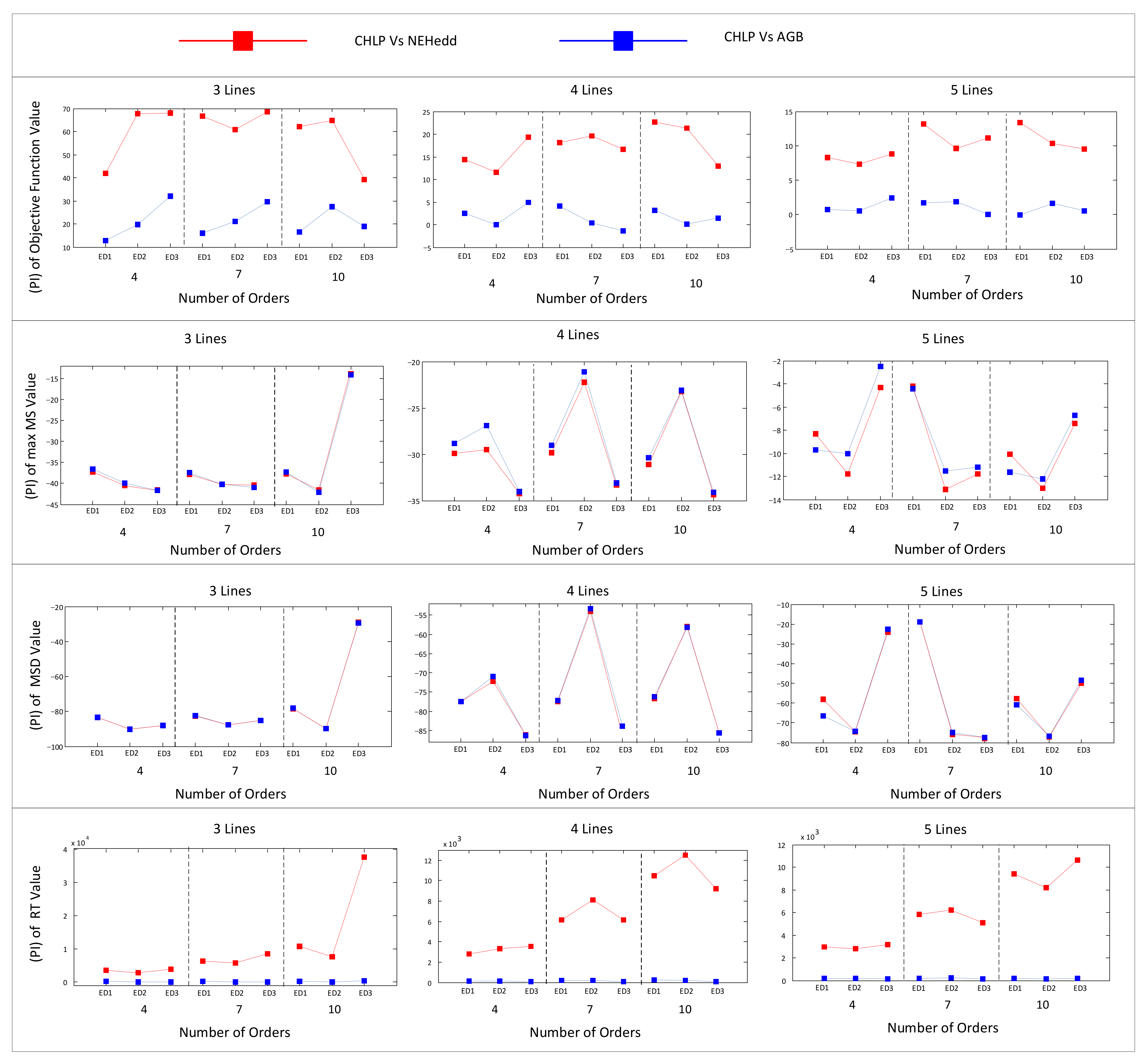
5.2.1. Percentage Improvements in Performance
The results obtained from proposed CHLP are compared with the results obtained from the AGB and NEHedd heuristics for all problem instances and presented in this section. The comparison of results is performed by measuring the values of objective (Obj), makespan (MS), makespan deviation from the average value of makespan of all lines (MSD) and run time (RT) of the proposed CHLP for all problem instances with the corresponding values obtained from AGB and NEHedd heuristics. The comparison is performed using the relation indicated in Equation (30):
where, indicates the percentage improvement of the comparison value of parameter x, i.e., x represents the objective, maximum makespan of the lines, makespan deviation of all lines and run time of the AGB and NEHedd heuristic algorithms. The comparison of percentage improvement in the value Obj, MS, MSD and RT is indicated in Table 5. The percentage improvement value is positive number for the maximizing objective function. Whereas the negative values of percentage improvement is for the minimizing metrics, i.e., (MS), (MSD) and (RT).
Improvement in Objective Function
It can be seen from Table 5 that the percentage increase in the value of objective obtained from the proposed CHLP is greater than zero for all problem instances as compared to the NEHedd. Besides, AGB heuristics, except for one instance in which AGB gives a better objective value (by only 0.1 percent) in the problem containing 10 lines, loose due date and have demand ED1, i.e., 5 to 15 demands in each customer order. These results indicate that the proposed CHLP is significant to solve lotsizing and scheduling on multiple lines and complete all customer orders within their corresponding due dates and gives the maximum probability to complete customer orders within their due dates. For instance, for three line problems, the maximum percentage improvement in objective value obtained is about 70.1 percent when the objective function value is compared with the value of the NEHedd heuristic for a problem containing 10 customer orders and due date is tight and demand is ED1, i.e., in the range of 5 to 15 products in every order, as highlighted in Table 5. Similarly, in the three lines problem; the maximum improvement in the objective value is 44.9 percent when the results are compared with the results of the AGB heuristic. This improvement is observed for the problem when there are four customer orders and the demand in each customer order is ED3, i.e., in the range of 35 to 45 products in each customer order. Similar results are obtained when comparing the objective function improvement from the proposed CHLP heuristic when compared with the NEHedd and AGB heuristic for four line and five line problems.
Improvement in Maximum Makespan (MS) of Lines
The results of the average improvement in the maximum value of the makespan among the lines after lotsizing and scheduling, illustrated in Table 5, indicate that the proposed CHLP performs better as compared to the NEHedd and AGB heuristics in most of the problem instances which are observed in the proposed experiments. It can be seen from Table 5 that the maximum improvement in the maximum makespan of the line is seen when CHLP is compared with NEHedd, giving 41.6 percent, 35.9 percent and 11.8 percent improvements in the average results obtained for three, four and five production line problem instances. Moreover, 42.1, 34.2 and 12.2 percent improvement in the maximum makespan of lines is observed when the lotsizing and scheduling results obtained from CHLP are compared with the results obtained from the AGB heuristic for three, four and five line problem instances. These results indicate that the proposed CHLP can give a lotsizing schedule which have smaller value of makespan of the lines and the maximum makespan of any line is also less than the maximum makespan obtained with the AGB heuristic in multiple lines.
Improvement in Makespan Deviation of Lines (MSD)
The results obtained from the proposed CHLP heuristic are compared with the NEHedd and AGB heuristics by comparing the balancing of makespan among lines when the schedule is made by these heuristics. It can be seen from Table 5 that the proposed CHLP gives a significant improvement when makespan deviation of lines from the average makespan of lines is observed. For instance, there is maximum of 90.1, 88.2 and 81 percent improvement in the makespan deviation when the results of problem instance with three lines, four lines and five lines respectively are compared with the NEHedd heuristic. Moreover, there is maximum of 90.1, 88.3 and 80.1 percent improvement in the makespan deviation when the lotsizing and scheduling results obtained from the proposed CHLP heuristic are compared with the results obtained from the AGB heuristic for three lines, four lines and fine lines problem instances, respectively. These results indicate that the proposed CHLP heuristic excels at improving the balancing of workload among multiple lines and all lines are completing the assigned product lots in similar completion times in the planning horizons. These results have significant application in shops with multiple lines, since it can reduce the overutilization of some lines and helps improve the uniform utilization of all lines.
Improvement in Run Time of Heuristics (RT)
The performance of the proposed CHLP heuristic is compared by measuring the percentage improvement in the run time of the heuristic as compared to the NEHedd and AGB heuristics. The results indicated in Table 5 shows that the proposed CHLP takes more run time as compared to the NEHedd and AGB heuristics. For instance, the minimum percentage increase in the run time of the proposed CHLP heuristic as compared to run time of NEhHedd heuristic is about 921, 949 and 721 for problems containing three lines, four lines and five lines, respectively. However, for the same problem instances there is about 47.9, 17, and 8.6 percent improvement in objective function (Obj) values, 40, 28.7 and 6.7 percent improvement in maximum makespan (MS) improvement and 87.5, 75.7 and 43.7 percentage improvement in makespan deviation (MSD) of the lines when compared for three lines, four lines and five lines problem instances. Similarly, the minimum value of the percentage improvement in the run time of the proposed CHLP heuristic is 38.9, 74.6 and 121.7 for problems containing three lines, four lines and five lines, respectively when compared with AGB heuristic. However this increase in run time can be compensated when the percentage improvements in objective function (Obj), maximum makespan (MS) and makespan deviation (MSD) of lines are analyzed. For the same problems instances, there is there is 31.9, 3.1 percent improvement in (Obj) for problems instances of three lines and four lines. However, the objective function value is the same for five lines problems. Moreover, there is a 41.7, 33.1, 11.2 percentage improvement in the maximum makespan (MS) for the problems with three lines, four lines and five lines, respectively. Furthermore, for the same problems instances, there is 88.2, 83.9 and 77.5 percentage improvement in the makespan deviation (MSD) of CHLP as compared to the AGB heuristic. The proposed CHLP takes more run time as compared to the NEHedd and AGB heuristics but at the same time it improves (Obj), (MS), and (MSD) for all problems instances by significant percentage values.
5.2.2. Graphical Results
The graphical representation of results for the proposed CHLP heuristic, AGB and NEHedd heuristics for tight due dates and for loose due dates are presented in this section.
Tight Due Date
The results of the considered problems containing tight due dates to measure the performance of the proposed CHLP heuristic are presented in Figure 5. There are three different combinations which can show the performance of the proposed CHLP algorithm when the parameters of the problem is changed. For example, the performance of CHLP when the demand range of the customers increases, when the number of customer orders increases and when the number of lines are increased. Three possible structures of the problem are analyzed in this section:
- (i)
- Fixed number of lines, fixed number of orders and varying demand range
The results indicated in Figure 5 illustrate that there is increase in the percentage improvement in performance with respect to (Obj) of CHLP against NEHedd, when the demand range increases from ED1 to ED2 and ED3 for problems containing four customer orders. However, there is decreasing pattern of the value of percentage improvement of (Obj) when the demand range increases from ED1 to ED2 and ED3 for the problems containing seven and ten orders. These results indicate that as the problem complexity increases with the increase in the number of customer orders, the performance of the proposed CHLP heuristic decreases slightly when compared with the NEHedd heuristic results. When the performance of CHLP is compared with AGB with respect to (Obj), it can be seen from Figure 5 that there is increasing pattern in the value of percentage improvement in (Obj) when the demand increases from ED1, to ED2 and ED3 for each specific lines problem containing a specific number of customer orders.
The results show that the value of percentage increase in (MS) is better if the value is more negative. There is decrease in the percentage improvement value of (MS) when the demand range increases from ED1 to ED2 and ED3 for problems containing three lines. Moreover, there is decreasing pattern in the performance of CHLP with respect to (MS) when compared with the NEHedd heuristic for problems containing four lines and when the demand range increases from ED1 to ED2 while the performance increases when the demand range increases to ED3. Similarly, for the problems with five lines, there is increasing pattern in the value of the percentage improvement in (MS) when the demand range increases from ED1 to ED2 and ED3 for four customer orders. However, for the problems containing seven and ten customer orders in the five line problem, there is decrease in the performance of CHLP with respect to (MS) as the demand range increases from ED2 to ED3. Similar results are observed when CHLP is compared with the AGB heuristic results.
The results show the value of percentage increase in (MSD) is better if the value is more negative. The percentage increase in the performance with respect to (MSD) shows that there is decreasing pattern of its values for CHLP when compared with NEHedd when the demand range increases from ED1 to ED2 and ED3 for problems containing three lines. However, when there are five lines, there is increasing pattern of the (MSD) values for CHLP as compared to the NEHedd heuristic. These results indicate that as the range of demand increases for a three lines problem the proposed algorithm performance decreases. However, there is increase in the performance value when the demand range increases for problems containing five lines. Similar results are observed when the CHLP is compared with the AGB heuristic, as can be seen from Figure 5.
The results showing the value of percentage increase in (RT) are better if the value is more negative. The percentage increase in the performance with respect to (RT) value of CHLP with respect to NEHedd heuristic as indicated in Figure 5 shows that there is increasing pattern in the value of (RT) of the proposed CHLP heuristic as the demand range increases from ED1 to ED2 and ED3 for problems containing either four, seven or ten orders with three lines or four lines or five lines. These results indicate that the proposed CHLP is not better than NEDedd with respect to (RT) in all problem instances. However, when the performance of the proposed CHLP is compared with the performance of the AGB heuristic as indicated in Figure 5, there is very less decrease in the (RT) when the demand range of problems increases from ED1 to ED2 and ED3. This shows that the performance of proposed CHLP is not better than that of AGB with respect to (RT), but its performance improves as the demand increases from ED1 to ED2 and ED3.
- (ii)
- Fixed number of lines, fixed demand range and varying number of orders
The results indicated in Figure 5 illustrate that when there is an increase in the number of orders while keeping the demand range and number of lines fixed, there is increasing pattern of the (Obj) values of CHLP as compared to the NEHedd heuristic when the customer orders are increased from four to seven and ten. However, there is slight decreasing pattern in the value of (Obj) when the results are compared for CHLP and AGB and number of customer orders are increased from four to seven and ten for a fixed number of lines and for a specific range of the demand. These results indicate that the proposed CHLP performs better than the AGB heuristic with respect to (Obj) for the problems containing small and medium ranges of numbers of orders while it decreases slightly when the number of orders is increased.
The results showing the value of percentage increase in (MS) are better if the value is more negative. Results indicated in Figure 5 illustrate that there is a decreasing pattern of percentage improvement (i.e., becoming a more positive value) with respect to (MS) of the proposed CHLP heuristic when the number of customer orders are increased from four to seven for a fixed range of demand and a fixed number of lines, when compared with NEHedd. Similar results are obtained when the percentage improvement of (MS) is observed for CHLP with AGB. These results indicate that the proposed CHLP is better in performance with respect to (MS) for the problems when number of orders are increased to ten. However, the overall percentage increase in performance value with respect to (MS) of proposed CHLP shows that it performs better as compared to the NEHedd and AGB heuristics.
The results indicated in Figure 5 show that, as the number of customer orders is increased for problems containing a fixed number of production lines and for a fixed range of demand, there is increase in the value of percentage increase in (RT) value of CHLP with respect to the NEHedd heuristic. These results shows that there is increasing pattern in the value of (RT) of the proposed CHLP heuristic as customer orders are increased from four to seven or ten. These results indicate that the proposed CHLP is not better than NEDedd with respect to (RT) in all problem instances. However, when the performance of the proposed CHLP is compared with the performance of the AGB heuristic as indicated in Figure 5, there is very less decrease in the (RT) when the number of orders are increased from to seven or ten. This shows that the performance of the proposed CHLP is not significant as compared to AGB in with respect to (RT), but its performance improves as the orders are increased from four to seven and ten.
- (iii)
- Fixed demand range, fixed number of orders and varying number of lines
The results indicted in Figure 5 illustrate that the percentage increase in the performance of the proposed CHLP with respect to (Obj) against the NEHedd heuristic decreases when the number of production lines are increased keeping demand and number of customer orders at a fixed number. Similar results are observed when the percentage increase in the value of (Obj) is observed for the proposed CHLP against the AGB heuristic. These results indicate that as there are more lines, the performance of the proposed CHLP decreases as compared to its performance when solving problems with a lesser number of lines.
The results presented in Figure 5 show that the values of the percentage increase in (MS) are better if the value is more negative. It can be seen from Figure 5 that as the number of lines is increased from three to four and five, for a fixed number of customer orders and fixed size of demand, there is decreasing pattern of the percentage increase in (MS). These results indicate that when the number of lines are increased in lotsizing and scheduling problems, the performance of the proposed CHLP decreases with respect to (MS) when compared with NEHedd and AGB. However, the overall performance of the proposed CHLP with respect to NEHedd and AGB is better at all of the problem instances considered.
Results showing the value of percentage increase in (MSD) are better if the value is more negative. Results shown in Figure 5 indicate that there is decreasing pattern in the percentage improvement of (MSD) of the CGLP as the number of lines are increased from three to four and five. However, the overall results indicate that the proposed CHLP gives better results with respect to (MSD) as compared to NEHedd and AGB.
Figure 5 shows that there is increasing pattern in the value of (RT) of the proposed CHLP heuristic as number of lines are increased from three to four and five when percentage increase of (RT) of CHLP is compared against the NEHedd heuristic. These results indicate that the NEDedd performs better than CHLP with respect to (RT) in all problem instances. However, when the performance of the proposed CHLP is compared with the performance of the AGB heuristic as indicated in Figure 5, there is a very small decrease in the (RT) when the number of lines is increased. This shows that the performance of AGB is better as compared to CHLP with respect to (RT).
Loose Due Date
The results obtained for the loose due date problem instances are indicated in Figure 6. These results shows the similar pattern of the performance of the proposed CHLP against NEHedd and AGB heuristics as given for the tight due date scenario.
5.2.3. Mean and Standard Deviation of Results
The summary of results of the proposed CHLP heuristic with NEHedd and AGB heuristics showing the mean and standard deviation of the values of Obj, MS and MSD are indicated in Table 6. It can be seen from Table 6 that in most of the instances of each problem, the mean value and standard deviation in the values of Obj, MS and MSD which are obtained from proposed CHLP heuristic are better as compared to the corresponding values obtained from NEHedd and AGB heuristics. These results indicate the better performance of the proposed CHLP heuristic against different problems instances and indicate the robustness of the proposed CHLP heuristic.
6. Conclusions
Dynamic lotsizing and scheduling problem in multiple production line environments is studied in the current research. Uncertain demand of customer orders in each planning horizon is scheduled on multiple lines considering mixed model products. The current research developed a mixed integer programming model considering uncertain demand, due date of customer orders, uncertain failure of machines on the production lines and sequence dependent setup time among different product models, with an aim to maximize the probability of completion of different product demands from customer orders on all production lines in the planning horizon. A constructive heuristic is developed to solve the current problem. The proposed heuristic includes some steps which can distribute different product lots among lines and balance the makespan between the lines. The performance of the proposed heuristic is tested against the performance of some famous scheduling heuristics in the literature using different size lotsizing and scheduling problems as case studies. The results indicate that the proposed CHLP gives a significant improvement to give maximum product models completed in their due date as compared to the NEHedd and AGB heuristics. In addition, the proposed CHLP gives a significant improvement in the maximum makespan of the lines as compared to the maximum makespan of lines obtained in NEHedd and AGB heuristics.
The proposed CHLP heuristic gives optimal results to reduce the makespan deviation of the lines from the average makepan on lines which is significant to describe the performance of proposed CHLP heuristic to balance the makespan among multiple lines. The performance of the proposed CHLP heuristic based on the run time (RT) is not significant as compared to the NEHedd and AGB heuristics however, the percentage improvements in the objective function value obtained from CHLP against the NEHedd and AGB heuristics are significant. Moreover, the percentage improvement in the maximum makespan of lines and percentage improvement of the makespan deviation of lines with the proposed CHLP is significantly better as compared to the NEHedd and AGB heuristics. In order to achieve fast convergence, future research can be extended to integrate the heuristics with intelligent algorithms (e.g., genetic algorithm, spider monkey optimization and artificial bee colony algorithm) to assign the load distribution among lines for further improvement in the performance of the heuristic.
Author Contributions
L.Y. leaded the research group and carried out the research work and drafted the manuscript. S.U. proposed a novel algorithm named CHLP and helped to implement all the experiments and analyze the experimental results in detail. J.M. helped to do some work of data processing. J.M., Y.C. and S.U. helped in literature review, make some revisions of the manuscript and give a lot of valuable suggestions. All authors have read and agreed to the published version of the manuscript.
Funding
This work has been supported by MOST (Ministry of Science & Technology of China) the Funds for International Cooperation and Exchange of the National Natural Science Foundation of China (No. 51561125002), the National Natural Science Foundation of China (No. 51905196).
Institutional Review Board Statement
Not applicable.
Informed Consent Statement
Not applicable.
Data Availability Statement
Not applicable.
Conflicts of Interest
The authors declare that they have no competing interest.
Abbreviations
| Index used to represent a planning horizon, | |
| o | Index used to represent customer order, |
| Index used to represent the flexible line, | |
| Index used to represent the position of lot of model | |
| Number of total lots from all models in line , | |
| Index used to represent the position of lot of model in line | |
| Index used to represent the sector in production line in line, | |
| Demand of product model in order which needs scheduling in planning horizon | |
| Demand of product model in order which is not completed in planning horizon | |
| Process time of process in product model | |
| Cycle time of the line if only model is produced on it in planning horizon | |
| Sum of cycle time due to model when it is produced on any line independently in planning horizon | |
| The allowed demand of a model which can be assigned to line in planning horizon | |
| The allowed demand of a model from order which can be assigned to line in planning horizon | |
| The greater common number of [ ] of model among all orders on a line in planning horizon | |
| Maximum integer value of which can be divisible by | |
| The number of lots of model from order which can be assigned to line in time horizon | |
| The lot size of model for order on line in time horizon and the lot is positioned at position in the lot schedule on line | |
| Total number of lots of model for order which are not completed in planning horizon and are added to planning horizon | |
| The number of lots of model for order which are to be sequence in planning line in planning horizon | |
| Duration of time in each planning horizon in line | |
| Number of shifts of work in one day | |
| Number of hours for each working shift | |
| Total time available on line for day in horizon , | |
| Number of days in planning horizon | |
| Start time on line for day in planning horizon | |
| The number of planning horizons passed before a planning horizon | |
| The repair rate of the machine in a cell of sector | |
| The failure rate of the machine in a cell of sector | |
| Number of days which have been passed from planning horizon | |
| Estimated average demand of model in order during the planning horizon | |
| Probability of occurrence of factor to change the demand of model in order during planning horizon in scenario | |
| The possible change in the demand of model in order due to the factor if it occurs before planning horizon in scenario | |
| Average value of demand of product model in order which needs scheduling in planning horizon | |
| Average value of demand of product model in order which is not completed in planning horizon | |
| Average allowed demand of a model which can be assigned to line in planning horizon | |
| Average allowed demand of a model from order which can be assigned to line in planning horizon | |
| Greater common number of of model among all orders on line in planning horizon | |
| Maximum integer value of which can be divisible by | |
| Average of number of lots of model from order which can be assigned to line in time horizon | |
| Average value of lot size of model for order on line in horizon and the lot is positioned at position in the lot schedule | |
| Average value of total number of lots of model for order which are not completed in planning horizon and are added to the planning horizon | |
| Average value of number of lots of model for order which are to be sequence in planning line in planning horizon | |
| Normal distributed due date of model from an order in planning horizon , | |
| Mean value of due date of the model from an order in planning horizon | |
| Variance value of due date of the model from an order in planning horizon | |
References
- He, C.; Guan, Z.; Xu, G.; Yue, L.; Ullah, S. Scenario-based robust dominance criteria for multi-objective automated flexible transfer line balancing problem under uncertainty. Int. J. Prod. Res. 2020, 58, 1–20. [Google Scholar] [CrossRef]
- He, C.; Guan, Z.; Yue, L.; Ullah, S. Set-partitioning-based heuristic for balancing and configuration of automated flexible machining line. Int. J. Prod. Res. 2018, 56, 3152–3172. [Google Scholar] [CrossRef]
- He, C.; Guan, Z.; Luo, D.; Fang, W.; Ullah, S. Decomposition heuristic for parallel-machine transfer line design with dual-uncertainties-based chance constraints. Eng. Optim. 2018, 51, 199–216. [Google Scholar] [CrossRef]
- Liu, X.; Li, A.; Chen, Z. Optimization of line configuration and balancing for flexible machining lines. Chin. J. Mech. Eng. 2016, 29, 579–587. [Google Scholar] [CrossRef]
- Brahimi, N.; Dauzère-Pérès, S.; Najid, N.M.; Nordli, A. Single item lotsizing problems. Eur. J. Oper. Res. 2006, 168, 1–16. [Google Scholar] [CrossRef]
- Darvish, M.; Larrain, H.; Coelho, L.C. A dynamic multi-plant lot-sizing and distribution problem. Int. J. Prod. Res. 2016, 54, 1–11. [Google Scholar] [CrossRef]
- Ferreira, D.; Morabito, R.; Rangel, S. Solution approaches for the soft drink integrated production lotsizing and scheduling problem. Eur. J. Oper. Res. 2009, 196, 697–706. [Google Scholar] [CrossRef]
- Yue, L.; Guan, Z.; Zhang, L.; Saif, U.; Cui, Y. Multi objective lotsizing and scheduling with material constraints in flexible parallel lines using a Pareto based guided artificial bee colony algorithm. Comput. Ind. Eng. 2019, 128, 659–680. [Google Scholar] [CrossRef]
- Glock, C.H.; Grosse, E.H.; Ries, J.M. The lotsizing problem: A tertiary study. Int. J. Prod. Econ. 2014, 155, 39–51. [Google Scholar] [CrossRef]
- Karimi-Nasab, M.; Seyedhoseini, S. Multi-level lotsizing and job shop scheduling with compressible process times: A cutting plane approach. Eur. J. Oper. Res. 2013, 231, 598–616. [Google Scholar] [CrossRef]
- Parveen, S.; Hasin, A.A. A Heuristic Solution of Multi-Item Single Level Capacitated Dynamic Lot-Sizing Problem with Setup Time. Adv. Mater. Res. 2011, 264, 1794–1801. [Google Scholar] [CrossRef] [Green Version]
- Hajipour, V.; Kheirkhah, A.; Tavana, M.; Absi, N. Novel Pareto-based meta-heuristics for solving multi-objective multi-item capacitated lot-sizing problems. Int. J. Adv. Manuf. Technol. 2015, 80, 31–45. [Google Scholar] [CrossRef]
- Masmoudi, O.; Yalaoui, A.; Ouazene, Y.; Chehade, H. Lot-sizing in a multi-stage flow line production system with energy consideration. Int. J. Prod. Res. 2016, 55, 1–23. [Google Scholar] [CrossRef]
- Seeanner, F.; Almada-Lobo, B.; Meyr, H. Combining the principles of variable neighborhood decomposition search and the fix&optimize heuristic to solve multi-level lot-sizing and scheduling problems. Comput. Oper. Res. 2013, 40, 303–317. [Google Scholar] [CrossRef]
- Sifaleras, A.; Konstantaras, I. Variable neighborhood descent heuristic for solving reverse logistics multi-item dynamic lot-sizing problems. Comput. Oper. Res. 2017, 78, 385–392. [Google Scholar] [CrossRef]
- Erdirik-Dogan, M.; Grossmann, I.E. Simultaneous planning and scheduling of single-stage multi-product continuous plants with parallel lines. Comput. Chem. Eng. 2008, 32, 2664–2683. [Google Scholar] [CrossRef] [Green Version]
- Meyr, H.; Mann, M. A decomposition approach for the General Lotsizing and Scheduling Problem for Parallel production Lines. Eur. J. Oper. Res. 2013, 229, 718–731. [Google Scholar] [CrossRef]
- Yan, H.S.; Wang, H.X.; Zhang, X.D. Simultaneous batch splitting and scheduling on identical parallel production lines. Inf. Sci. 2013, 221, 501–519. [Google Scholar] [CrossRef]
- Essafi, M.; Delorme, X.; Dolgui, A.; Guschinskaya, O. A MIP approach for balancing transfer line with complex industrial constraints. Comput. Ind. Eng. 2010, 58, 393–400. [Google Scholar] [CrossRef]
- Essafi, M.; Delorme, X.; Dolgui, A. A reactive GRASP and Path Relinking for balancing reconfigurable transfer lines. Int. J. Prod. Res. 2012, 50, 5213–5238. [Google Scholar] [CrossRef]
- Mumtaz, J.; Guan, Z.; Yue, L.; Wang, Z.; Ullah, S.; Rauf, M. Multi-level planning and scheduling for parallel PCB assembly lines using hybrid spider monkey optimization approach. IEEE Access. 2019, 7, 18685–18700. [Google Scholar] [CrossRef]
- Mumtaz, J.; Guan, Z.; Yue, L.; Zhang, L.; He, C. Hybrid spider monkey optimisation algorithm for multi-level planning and scheduling problems of assembly lines. Int. J. Prod. Res. 2020. [Google Scholar] [CrossRef]
- Khalid, Q.S.; Arshad, M.; Maqsood, S.; Jahanzaib, M.; Babar, A.R.; Khan, I.; Mumtaz, J.; Kim, S. Hybrid Particle swarm algorithm for products’ scheduling problem in cellular manufacturing system. Symmetry 2019, 729. [Google Scholar] [CrossRef] [Green Version]
- Nawaz, M.; Enscore, E.E.; Ham, I. A heuristic algorithm for the m-machine, n-job flow-shop sequencing problem. Omega 1983, 11, 91–95. [Google Scholar] [CrossRef]
- Mumtaz, J.; Zailin, G.; Mirza, J.; Rauf, M.; Sarfraz, S.; Shehab, E. Makespan minimization for flow shop scheduling problems using modified operators in genetic algorithm. In Advances in Manufacturing Technology XXXII, Proceedings of the 16th International Conference on Manufacturing Research, ICMR, Skövde, Sweden, 11–13 September 2018; IOS Press: Clifton, VA, USA, 2018. [Google Scholar] [CrossRef]
- Framinan, J.M.; Leisten, R.; Rajendran, C. Different initial sequences for the heuristic of Nawaz, Enscore and Ham to minimize makespan, idletime or flowtime in the static permutation flowshop sequencing problem. Int. J. Prod. Res. 2003, 41, 121–148. [Google Scholar] [CrossRef]
- Rauf, M.; Guan, Z.; Sarfraz, S.; Mumtaz, J.; Shehab, E.; Jahanzaib, M.; Hanif, M. A smart algorithm for multi-criteria optimization of model sequencing problem in assembly lines. Robot. Comput. Integr. Manuf. 2020, 61, 101844. [Google Scholar] [CrossRef]
- Vallada, E.; Ruiz, R. Genetic algorithms with path relinking for the minimum tardiness permutation flowshop problem. Omega 2010, 38, 57–67. [Google Scholar] [CrossRef]
- Laha, D.; Sarin, S.C. A heuristic to minimize total flow time in permutation flow shop☆. Omega 2009, 37, 734–739. [Google Scholar] [CrossRef]
- Abedinnia, H.; Glock, C.H.; Brill, A. New simple constructive heuristic algorithms for minimizing total flow-time in the permutation flowshop scheduling problem. Comput. Oper. Res. 2016, 74, 165–174. [Google Scholar] [CrossRef]
- Zimmer, W. An Introduction to Reliability and Maintainability Engineering. J. Qual. Technol. 1999, 31, 464–466. [Google Scholar] [CrossRef]
Figure 1.
Multiple flexible machining line shop.

Figure 2.
The procedures of the NEHedd heuristic.

Figure 3.
The procedures of the AGB heuristic.

Figure 4.
The procedures of the CHLP heuristic.

Figure 5.
Percentage improvement in different comparison metrics in tight due date instances.

Figure 6.
Percentage improvement in different comparison metrics in loose due date instances.


Table 1.
Structure of the experiments performed.
| Size of Problem with Number of Orders | Estimated Demand | Due Date | Number of Experiments | |
|---|---|---|---|---|
| 3, 4 and 5 Lines | 4 | Ed1 5~15 | Tight | 10 |
| Ed2 20~30 | 10 | |||
| Ed3 35~45 | 10 | |||
| 7 | Ed1 5~15 | 10 | ||
| Ed2 20~30 | 10 | |||
| Ed3 35~45 | 10 | |||
| 10 | Ed1 5~15 | 10 | ||
| Ed2 20~30 | 10 | |||
| Ed3 35~45 | 10 | |||
| 4 | Ed1 5~15 | Loose | 10 | |
| Ed2 20~30 | 10 | |||
| Ed3 35~45 | 10 | |||
| 7 | Ed1 5~15 | 10 | ||
| Ed2 20~30 | 10 | |||
| Ed3 35~45 | 10 | |||
| 10 | Ed1 5~15 | 10 | ||
| Ed2 20~30 | 10 | |||
| Ed3 35~45 | 10 |
Table 2.
Processing time data generated for each product model on each sector.
| Sector | Processing Time of Product Model | |||
|---|---|---|---|---|
| A | B | C | D | |
| 1 | 18 | 53 | 55 | 5 |
| 2 | 3 | 44 | 54 | 62 |
| 3 | 55 | 47 | 21 | 49 |
| 4 | 16 | 4 | 2 | 48 |
| 5 | 31 | 45 | 49 | 52 |
| 6 | 55 | 45 | 49 | 48 |
| 7 | 8 | 15 | 60 | 59 |
| 8 | 20 | 45 | 53 | 60 |
| 9 | 34 | 20 | 32 | 64 |
| 10 | 29 | 21 | 29 | 46 |
Table 3.
Sequence dependent setup time between different product models on sectors.
| Sequence Dependent Setup Time between Different Product Models | ||||
|---|---|---|---|---|
| A | B | C | D | |
| A | 0 | 23 | 32 | 25 |
| B | 35 | 0 | 32 | 10 |
| C | 45 | 35 | 0 | 20 |
| D | 15 | 34 | 40 | 0 |
Table 4.
Cycle time of lines for each product model.
| Product Model | Cycle Time of Lines | ||||
|---|---|---|---|---|---|
| Line 1 | Line 2 | Line 3 | Line 4 | Line 5 | |
| A | 13 | 17 | 15 | 13 | 11 |
| B | 18 | 18 | 17 | 19 | 12 |
| C | 16 | 16 | 12 | 16 | 17 |
| D | 20 | 10 | 12 | 18 | 10 |
Table 5.
Comparison of results of percentage improvement of CHLP with NEHedd and AGB.
| Number of Lines | Size of Problem with Number of Orders | Estimated Demand | Due Date | Percentage Improvement of Average Values | |||||||
|---|---|---|---|---|---|---|---|---|---|---|---|
| CHLP vs. NEHedd | CHLP vs. AGB | ||||||||||
| Obj | MS | MSD | RT | Obj | MS | MSD | RT | ||||
| 3 Lines | 4 | ED1 | Tight | 47.9 | −40.0 | −87.5 | 921.2 | 18.5 | −38.9 | −87.2 | 170.1 |
| ED2 | 56.4 | −37.6 | −79.6 | 2377.2 | 39.1 | −36.5 | −79.2 | 69.8 | |||
| ED3 | 66.3 | −39.6 | −84.8 | 4215.1 | 44.9 | −39.6 | −84.9 | 35.2 | |||
| 7 | ED1 | 69.9 | −38.4 | −84.4 | 5687.7 | 25.4 | −37.6 | −84.1 | 221.8 | ||
| ED2 | 44.1 | −37.8 | −78.6 | 5936.7 | 34.7 | −37.4 | −78.6 | 57.6 | |||
| ED3 | 45.0 | −32.8 | −67.3 | 9643.1 | 33.2 | −32.0 | −67.1 | 55.5 | |||
| 10 | ED1 | 70.1 | −39.5 | −83.0 | 10,378.9 | 23.6 | −38.2 | −82.5 | 252.6 | ||
| ED2 | 59.9 | −29.5 | −61.5 | 12,997.7 | 42.7 | −29.0 | −61.3 | 129.3 | |||
| ED3 | 35.5 | −25.1 | −50.8 | 24,998.6 | 28.8 | −24.3 | −50.4 | 178.2 | |||
| 4 | ED1 | Loose | 41.9 | −37.3 | −83.4 | 3452.8 | 12.8 | −36.5 | −83.4 | 259.8 | |
| ED2 | 67.7 | −40.5 | −90.1 | 2703.1 | 19.8 | −39.9 | −90.1 | 61.0 | |||
| ED3 | 67.9 | −41.5 | −88.0 | 3840.2 | 31.9 | −41.7 | −88.2 | 38.9 | |||
| 7 | ED1 | 66.8 | −37.9 | −82.7 | 6334.8 | 16.1 | −37.4 | −82.5 | 227.5 | ||
| ED2 | 60.7 | −40.2 | −87.7 | 5704.3 | 21.2 | −40.3 | −87.8 | 51.7 | |||
| ED3 | 68.4 | −40.4 | −85.2 | 8505.5 | 29.5 | −40.9 | −85.4 | 35.8 | |||
| 10 | ED1 | 62.2 | −37.7 | −78.6 | 10,741.8 | 16.5 | −37.3 | −78.3 | 259.1 | ||
| ED2 | 64.7 | −41.6 | −89.8 | 7542.3 | 27.4 | −42.1 | −90.0 | 51.2 | |||
| ED3 | 39.1 | −13.8 | −29.1 | 37,597.4 | 18.9 | −14.1 | −29.6 | 326.5 | |||
| 4 Lines | 4 | ED1 | Tight | 17.1 | −28.7 | −75.7 | 949.1 | 2.6 | −27.3 | −74.5 | 189.4 |
| ED2 | 20.3 | −32.9 | −80.0 | 2624.0 | 4.4 | −32.0 | −79.6 | 105.5 | |||
| ED3 | 24.0 | −29.5 | −78.1 | 3214.8 | 3.7 | −29.2 | −78.3 | 85.6 | |||
| 7 | ED1 | 23.7 | −29.4 | −76.0 | 6114.8 | 0.8 | −27.9 | −75.0 | 207.5 | ||
| ED2 | 30.2 | −23.9 | −59.2 | 7932.9 | 7.7 | −23.7 | −59.7 | 236.5 | |||
| ED3 | 28.7 | −35.9 | −88.2 | 5910.0 | 2.6 | −35.7 | −88.3 | 79.9 | |||
| 10 | ED1 | 24.8 | −32.1 | −78.5 | 8440.6 | −3.0 | −29.9 | −77.2 | 173.1 | ||
| ED2 | 32.7 | −3.2 | −6.0 | 44,069.9 | 2.6 | −2.2 | −5.4 | 1034.0 | |||
| ED3 | 27.6 | −33.7 | −80.5 | 9484.7 | 2.7 | −33.0 | −80.3 | 86.3 | |||
| 4 | ED1 | Loose | 14.4 | −29.9 | −77.6 | 2827.7 | 2.6 | −28.8 | −77.5 | 163.4 | |
| ED2 | 11.6 | −29.5 | −72.3 | 3340.3 | 0.0 | −26.9 | −71.0 | 142.1 | |||
| ED3 | 19.3 | −34.2 | −86.1 | 3526.9 | 4.9 | −34.0 | −86.3 | 97.3 | |||
| 7 | ED1 | 18.1 | −29.8 | −77.6 | 6126.1 | 4.1 | −29.0 | −77.2 | 213.3 | ||
| ED2 | 19.6 | −22.2 | −54.0 | 8104.9 | 0.4 | −21.1 | −53.4 | 228.2 | |||
| ED3 | 16.7 | −33.3 | −83.9 | 6163.5 | −1.3 | −33.1 | −83.9 | 74.6 | |||
| 10 | ED1 | 22.7 | −31.1 | −76.7 | 10,499.9 | 3.2 | −30.4 | −76.2 | 234.7 | ||
| ED2 | 21.3 | −23.2 | −58.0 | 12,481.3 | 0.2 | −23.1 | −58.2 | 206.8 | |||
| ED3 | 13.0 | −34.4 | −85.7 | 9188.3 | 1.5 | −34.1 | −85.7 | 75.6 | |||
| 5 Lines | 4 | ED1 | Tight | 8.6 | −6.7 | −43.7 | 761.3 | 0.5 | −8.9 | −51.1 | 179.3 |
| ED2 | 6.5 | −11.5 | −66.9 | 3003.1 | 0.8 | −7.8 | −61.6 | 216.9 | |||
| ED3 | 8.7 | −12.9 | −81.0 | 2651.3 | 0.6 | −11.6 | −80.7 | 140.7 | |||
| 7 | ED1 | 13.9 | −5.5 | −29.3 | 5971.1 | 0.5 | −5.6 | −29.9 | 208.3 | ||
| ED2 | 13.3 | −11.4 | −70.9 | 5959.7 | 0.9 | −9.3 | −69.1 | 202.5 | |||
| ED3 | 12.7 | −6.3 | −45.4 | 6453.1 | 1.2 | −6.9 | −50.3 | 178.7 | |||
| 10 | ED1 | 18.3 | −11.0 | −59.9 | 9235.8 | 0.1 | −10.1 | −59.0 | 149.7 | ||
| ED2 | 13.0 | −12.3 | −76.6 | 8206.2 | 1.3 | −13.2 | −78.4 | 172.2 | |||
| ED3 | 12.6 | −7.9 | −48.9 | 9199.9 | 0.8 | −8.2 | −52.1 | 170.8 | |||
| 4 | ED1 | Loose | 8.3 | −8.3 | −58.0 | 2961.3 | 0.7 | −9.7 | −66.4 | 207.8 | |
| ED2 | 7.3 | −11.8 | −74.7 | 2775.7 | 0.6 | −10.0 | −74.1 | 196.7 | |||
| ED3 | 8.8 | −4.3 | −24.0 | 3181.7 | 2.4 | −2.5 | −22.5 | 152.9 | |||
| 7 | ED1 | 13.2 | −4.2 | −18.9 | 5815.2 | 1.7 | −4.4 | −19.0 | 180.5 | ||
| ED2 | 9.6 | −13.1 | −75.7 | 6204.7 | 1.9 | −11.5 | −74.8 | 217.0 | |||
| ED3 | 11.1 | −11.8 | −77.9 | 5114.8 | 0.0 | −11.2 | −77.5 | 121.7 | |||
| 10 | ED1 | 13.4 | −10.1 | −57.8 | 9437.1 | −0.1 | −11.6 | −61.0 | 195.0 | ||
| ED2 | 10.3 | −13.0 | −77.0 | 8166.4 | 1.6 | −12.2 | −76.8 | 147.9 | |||
| ED3 | 9.5 | −7.4 | −50.0 | 10,616.2 | 0.6 | −6.7 | −48.5 | 191.1 | |||
Table 6.
Summary of results of CHLP with NEHedd and AGB heuristics with mean and standard deviation of different comparison metrics.
Table 6.
Summary of results of CHLP with NEHedd and AGB heuristics with mean and standard deviation of different comparison metrics.
| 3 lines | Number of Orders | Obj (Mean/st dev) | MS (Mean/st dev) | MSD (Mean/st dev) | ||||||||
| Due Date | Estimated Demand | NEHedd | AGB | CHLP | NEHedd | AGB | CHLP | NEHedd | AGB | CHLP | ||
| Tight | 4 | ED1 | 98.30069/8.805509 | 122.7033/11.09783 | 145.363/11.51668 | 6365/374.2847 | 6251/430.014 | 3937/3879 | 1942.247/158.4479 | 1887.222/215.2157 | 242.336/39.51123 | |
| ED2 | 241.9174/12.7023 | 272.0703/6.101868 | 378.4128/2.690194 | 14,450/268.4176 | 14,212.33/59.5007 | 8071/10,254 | 4654.692/144.1209 | 4565.87/26.30892 | 948.9381/776.7566 | |||
| ED3 | 370.12/22.48565 | 424.5609/3.043784 | 615.3544/15.19337 | 22,301.33/266.7608 | 22,332.67/232.8011 | 13,347/13,551 | 7213.477/69.59767 | 7279.199/103.7511 | 1096.451/317.1472 | |||
| 7 | ED1 | 151.3666/19.44257 | 205.1331/29.66419 | 257.1959/21.90211 | 10,571.67/745.4276 | 10,440/774.5005 | 6366/7105 | 3319.956/332.9879 | 3271.732/308.8637 | 519.3126/156.3284 | ||
| ED2 | 424.6693/10.89009 | 454.2986/8.730234 | 611.927/24.99142 | 24,470/584.729 | 24,324/728.0103 | 15,631/14,711 | 7926.252/224.5686 | 7932.312/287.6652 | 1697.271/532.5862 | |||
| ED3 | 655.6315/9.865359 | 713.7382/35.58148 | 950.4292/42.46779 | 38,273.67/452.0048 | 37827.33/405.7861 | 29,352/23,896 | 12,414.1/132.4835 | 12,322.51/152.2046 | 4057.872/2085.727 | |||
| 10 | ED1 | 213.3345/38.65946 | 293.5006/61.6073 | 362.8687/31.01497 | 14,991.67/848.3845 | 14,672/689.0341 | 9177/8669 | 4775.778/386.3903 | 4648.156/236.5074 | 813.7396/427.2822 | ||
| ED2 | 525.0967/31.52382 | 588.3935/46.15789 | 839.7806/45.40211 | 34,798/780.6997 | 34,544.33/987.5152 | 20,698/20,223 | 11,385.96/262.9174 | 11,342.62/491.5525 | 4386.207/4616.978 | |||
| ED3 | 930.7582/35.9016 | 979.2619/31.81471 | 1261.452/138.1829 | 53,769.33/462.366 | 53,257.33/535.4497 | 32,658/34,302 | 17,533.45/137.4789 | 17,390.74/165.24 | 8623.126/7843.745 | |||
| Loose | 4 | ED1 | 106.8601/14.15599 | 134.4632/15.47817 | 151.6468/12.00317 | 6337/386.268 | 6262.333/396.056 | 4142/3908 | 1922.783/161.169 | 1925.801/172.5874 | 319.0499/91.56597 | |
| ED2 | 231.9278/20.43715 | 324.5913/14.34566 | 388.8865/6.336484 | 14,162.67/520.132 | 14,028/514.5804 | 8189/8434 | 4508.875/223.5418 | 4495.146/201.643 | 445.1314/73.91367 | |||
| ED3 | 373.6634/15.77202 | 475.6737/47.53367 | 627.2758/14.77915 | 22,253.67/299.6904 | 22,306.33/431.9911 | 12,290/13,334 | 7154.745/115.6829 | 7269.533/147.3897 | 857.8287/568.6008 | |||
| 7 | ED1 | 163.2034/14.48901 | 234.4145/26.81511 | 272.1514/25.15341 | 10,495.33/801.0626 | 10,409/857.1015 | 6358/6756 | 3305.563/325.1074 | 3266.751/368.5107 | 571.7457/276.2177 | ||
| ED2 | 406.0249/25.20067 | 538.2875/26.43672 | 652.4114/26.70992 | 24,263.67/908.5732 | 24,298/665.9782 | 13,766/14,701 | 7885.646/340.6954 | 7967.837/264.5755 | 972.9035/349.8923 | |||
| ED3 | 625.4002/15.59647 | 813.477/35.82453 | 1053.473/35.2672 | 37,854.67/744.4598 | 38,204/243.0453 | 22,326/22,483 | 12,307.92/273.3461 | 12,509.1/29.56552 | 1826.572/218.662 | |||
| 10 | ED1 | 233.7796/7.46183 | 325.4344/47.07676 | 379.122/33.66002 | 14,803.67/1020.941 | 14,701/760.0493 | 9171/9421 | 4715.211/409.7251 | 4670.36/305.1261 | 1011.196/306.9999 | ||
| ED2 | 570.0558/28.50975 | 737.0825/21.22441 | 938.8041/47.92858 | 34,110.67/992.76 | 34,424.33/1113.244 | 20,471/19,105 | 11,081.42/353.7797 | 11,274.93/514.3987 | 1128.314/415.1791 | |||
| ED3 | 932.5502/25.04013 | 1091.108/88.95119 | 1296.982/127.8959 | 53,412.33/640.8091 | 53,569/232.2692 | 51,903/32,273 | 17,475.12/217.2945 | 17,585.61/44.68807 | 12,381.86/8170.251 | |||
| 4 Lines | Obj (Mean/st dev) | MS (Mean/st dev) | MSD (Mean/st dev) | |||||||||
| Due Date | NEHedd | AGB | CHLP | NEHedd | AGB | CHLP | NEHedd | AGB | CHLP | |||
| Tight | 4 | ED1 | 131.0353/16.21232 | 149.446/13.8427 | 153.4025/14.86976 | 4470/414.8265 | 4385.667/267.3992 | 3187/340.8504 | 929.7472/186.8428 | 558.295/525.312739 | 225.5806/149.9639 | |
| ED2 | 324.7689/29.9919 | 374.0017/19.95983 | 390.5437/1.716956 | 9726/150.6884 | 9604/269.065 | 6528.333/438.7828 | 2155.57/86.8549 | 1121.21245/1462.802476 | 431.7854/249.0686 | |||
| ED3 | 513.6706/31.22009 | 614.4254/13.87401 | 637.1856/8.672091 | 14,787.67/229.147 | 14,728.33/307.9388 | 10,424/326.3847 | 3257.31/68.43677 | 1662.873385/2254.873885 | 714.3986/186.6623 | |||
| 7 | ED1 | 219.2725/32.16905 | 269.0035/18.46382 | 271.1675/26.20796 | 7287.333/706.8842 | 7137.667/539.6317 | 5146.333/642.6432 | 1563.6/256.7785 | 910.18925/924.0623445 | 375.4575/202.3528 | ||
| ED2 | 517.1811/5.983651 | 625.2066/26.9775 | 673.2117/21.20299 | 16,685.33/425.9112 | 16,633/435.0184 | 12,696/3020.387 | 3780.21/132.9458 | 1956.5779/2579.005249 | 1540.567/1608.493 | |||
| ED3 | 848.8244/49.53007 | 1064.301/46.23988 | 1092.113/18.94212 | 25,872/376.5541 | 25,780.67/571.6243 | 16,581.33/552.3697 | 5851.93/80.57266 | 2966.25133/4080.965912 | 692.7202/207.6469 | |||
| 10 | ED1 | 303.2771/28.98565 | 390.0198/30.49098 | 378.3959/28.95465 | 10,444.67/585.1447 | 10,117.67/489.9126 | 7088.333/248.1941 | 2352.787/229.5769 | 1291.18195/1501.33626 | 506.3133/113.6265 | ||
| ED2 | 709.2052/10.13574 | 917.4223/73.82233 | 941.2239/47.65802 | 23,639.67/765.0499 | 23,398.33/638.2682 | 22,892.67/1112.677 | 5444.252/237.3466 | 2840.7993/3681.838117 | 5116.229/511.1951 | |||
| ED3 | 1184.682/77.41377 | 1472.091/22.17651 | 1511.968/23.59451 | 36,208.67/388.6661 | 35,835.67/305.4592 | 24,022.67/1428.577 | 8259.55/115.4774 | 4187.5137/5758.728962 | 1607.266/960.0114 | |||
| Loose | 4 | ED1 | 135.9314/23.15391 | 151.6105/10.10216 | 155.4941/10.01251 | 4352.333/250.4123 | 4286/390.4164 | 3049.667/146.5481 | 869.4212/125.5756 | 497.4984/525.9782679 | 195.0537/37.40459 | |
| ED2 | 351.4379/8.28008 | 391.8987/8.560552 | 392.0529/2.88052 | 9803.333/286.0181 | 9457.333/102.4711 | 6908.667/1162.336 | 2181.47/116.6672 | 1149.0686/1460.036062 | 603.7919/700.4235 | |||
| ED3 | 534.8733/8.195164 | 608.1883/21.49875 | 638.2901/7.543234 | 14,983/468.8784 | 14,942.33/509.5393 | 9862/233.4502 | 3325.595/186.5128 | 1756.0539/2219.66631 | 460.953/125.6402 | |||
| 7 | ED1 | 235.3136/34.91052 | 267.0246/12.95698 | 277.9374/17.81231 | 7189.333/455.8644 | 7113.667/608.1458 | 5048/341.4045 | 1538.65/134.7879 | 836.71895/992.6804108 | 344.9685/14.19927 | ||
| ED2 | 572.4744/23.90695 | 681.5578/12.27753 | 684.4853/13.70988 | 16,473.33/579.9365 | 16,240.67/304.1157 | 12,818.33/3131.645 | 3732.693/172.5077 | 1952.60035/2517.431168 | 1718.757/1726.647 | |||
| ED3 | 926.1324/25.91612 | 1095.188/20.9098 | 1081.058/5.768284 | 25,477.67/668.325 | 25,388.67/772.2217 | 16,985/491.3685 | 5770.219/226.0407 | 2998.12985/3920.326072 | 926.1697/174.3971 | |||
| 10 | ED1 | 321.925/41.55316 | 383.0559/28.64586 | 395.1549/31.49687 | 10,244.67/576.6145 | 10,137/722.6977 | 7054.667/249.079 | 2286.733/169.8591 | 1228.29605/1496.85589 | 533.6533/50.54317 | ||
| ED2 | 798.6711/55.56843 | 966.8506/42.39568 | 968.6191/41.43664 | 22,988/620.8969 | 22,948.33/461.5153 | 17,656/5082.252 | 5186.625/183.641 | 2685.133/3537.643913 | 2179.587/2757.538 | |||
| ED3 | 1357.591/48.26468 | 1511.269/72.89519 | 1534.193/22.96325 | 35,762/465.2236 | 35,612.33/539.1125 | 23,463/1010.409 | 8144.282/190.9807 | 4167.63135/5623.833282 | 1161.839/492.194 | |||
| 5 Lines | Obj (Mean/st dev) | MS (Mean/st dev) | MSD (Mean/st dev) | |||||||||
| Due Date | NEHedd | AGB | CHLP | NEHedd | AGB | CHLP | NEHedd | AGB | CHLP | |||
| Tight | 4 | ED1 | 145.9126/17.20629 | 157.5952/14.79429 | 158.4038/14.75752 | 2699/362.7768 | 2764/275.768 | 2517/38.50974 | 174.8855/152.2068 | 201.181/132.7901 | 98.46005/40.47307 | |
| ED2 | 374.4117/11.64663 | 395.6215/11.57878 | 398.8205/8.022793 | 5793.333/153.5459 | 5560/357.6045 | 5127.333/124.5003 | 470.4965/63.272 | 405.4091/119.5518 | 155.5621/57.7118 | |||
| ED3 | 587.2381/13.47961 | 634.5735/7.885983 | 638.3423/7.562415 | 8610.333/185.1333 | 8479.667/163.3595 | 7497.667/171.7042 | 649.1583/40.04768 | 638.9552/45.61476 | 123.5799/61.2556 | |||
| 7 | ED1 | 247.4229/31.29884 | 280.5352/29.47315 | 281.8378/26.7103 | 4470.667/806.9457 | 4475.333/705.2917 | 4223.333/280.2612 | 372.2251/281.1234 | 375.6942/225.1135 | 263.2997/28.3264 | ||
| ED2 | 607.9853/23.67503 | 682.9668/17.97563 | 689.0429/23.70814 | 9574/616.3254 | 9358.667/475.1593 | 8484.667/497.9371 | 757.8886/213.2966 | 713.0017/164.7897 | 220.28/93.57722 | |||
| ED3 | 984.5027/5.913745 | 1096.311/12.22493 | 1109.804/18.02737 | 14,534.67/57.55287 | 14,627/248.4572 | 13,622.67/1261.491 | 1072.006/48.32254 | 1177.573/71.47694 | 585.5776/718.6654 | |||
| 10 | ED1 | 340.2242/18.87202 | 402.1017/28.91182 | 402.6325/30.6042 | 6211.667/785.127 | 6152.667/673.3389 | 5529.333/394.3176 | 533.4571/327.926 | 522.0718/236.6907 | 213.9415/101.7822 | ||
| ED2 | 870.0056/43.49199 | 970.1003/30.2398 | 982.9199/24.07401 | 13,407.67/582.5782 | 13538.67/582.6159 | 11,754.33/248.0934 | 1079.066/144.4753 | 1173.049/201.0817 | 252.9395/42.20527 | |||
| ED3 | 1383.43/3.751009 | 1545.548/17.87581 | 1558.11/8.566746 | 20,486/144.6548 | 20569/204.2645 | 18,874/1086.934 | 1571.703/64.23916 | 1678.541/37.04511 | 803.3282/533.709 | |||
| Loose | 4 | ED1 | 147.8245/10.80962 | 158.9191/13.02556 | 160.0724/12.32926 | 2713.667/224.745 | 2755.333/360.5348 | 2487.667/32.53204 | 177.9844/121.1993 | 222.8995/154.8501 | 74.78472/54.28138 | |
| ED2 | 370.0929/8.805307 | 394.5455/1.426947 | 396.9857/4.083499 | 5651.667/377.5398 | 5537.333/419.487 | 4982.667/144.1608 | 413.7897/131.3603 | 405.0999/136.8476 | 104.8372/22.5418 | |||
| ED3 | 585.5686/13.22419 | 622.2132/3.212596 | 637.2478/8.599257 | 8669.667/191.0009 | 8509.333/208.4234 | 8293.333/630.0987 | 661.6781/60.61277 | 649.4155/38.98743 | 503.081/283.4154 | |||
| 7 | ED1 | 254.2467/20.19223 | 282.8408/25.45986 | 287.7858/25.72242 | 4488.333/683.4452 | 4497.333/777.8344 | 4300.667/912.6869 | 389.4603/226.3066 | 390.1248/293.7321 | 315.8395/356.3582 | ||
| ED2 | 631.9312/10.31775 | 680.1465/20.52576 | 692.8541/12.92979 | 9574.333/553.285 | 9398.333/534.3934 | 8320.333/360.9118 | 786.8311/167.4663 | 758.525/171.0733 | 191.4041/87.03816 | |||
| ED3 | 995.9665/19.62842 | 1106.991/7.529752 | 1106.74/10.89207 | 14,641/187.3579 | 14,529.33/224.7495 | 12,908.33/320.0396 | 1160.101/13.34137 | 1138.011/4.8822 | 256.2655/80.28898 | |||
| 10 | ED1 | 356.006/26.81341 | 403.8773/24.27805 | 403.5782/22.18911 | 6129.333/698.7255 | 6233/730.6347 | 5509.333/507.8005 | 516.609/227.6712 | 558.2223/286.806 | 217.8841/143.5481 | ||
| ED2 | 885.8731/17.13584 | 961.7243/31.67613 | 977.1258/23.04813 | 13,347/691.3906 | 13,221/621.4298 | 11,612.67/403.9509 | 1075.922/174.6897 | 1064.934/161.0458 | 247.0421/81.43055 | |||
| ED3 | 1431.314/34.7938 | 1556.648/33.54151 | 1566.758/11.34253 | 20,511/155.9647 | 20,359.33/156.0716 | 18,989.67/1425.944 | 1658.72/70.64056 | 1611.732/31.08996 | 830.088/707.8564 | |||
Publisher’s Note: MDPI stays neutral with regard to jurisdictional claims in published maps and institutional affiliations. |
© 2021 by the authors. Licensee MDPI, Basel, Switzerland. This article is an open access article distributed under the terms and conditions of the Creative Commons Attribution (CC BY) license (https://creativecommons.org/licenses/by/4.0/).
Share and Cite
MDPI and ACS Style
Yue, L.; Chen, Y.; Mumtaz, J.; Ullah, S. Dynamic Mixed Model Lotsizing and Scheduling for Flexible Machining Lines Using a Constructive Heuristic. Processes 2021, 9, 1255. https://0-doi-org.brum.beds.ac.uk/10.3390/pr9071255
AMA Style
Yue L, Chen Y, Mumtaz J, Ullah S. Dynamic Mixed Model Lotsizing and Scheduling for Flexible Machining Lines Using a Constructive Heuristic. Processes. 2021; 9(7):1255. https://0-doi-org.brum.beds.ac.uk/10.3390/pr9071255
Chicago/Turabian StyleYue, Lei, Yarong Chen, Jabir Mumtaz, and Saif Ullah. 2021. "Dynamic Mixed Model Lotsizing and Scheduling for Flexible Machining Lines Using a Constructive Heuristic" Processes 9, no. 7: 1255. https://0-doi-org.brum.beds.ac.uk/10.3390/pr9071255
Note that from the first issue of 2016, this journal uses article numbers instead of page numbers. See further details here.