
A Lagrange Relaxation Based Decomposition Algorithm for Large-Scale Offshore Oil Production Planning Optimization


1
Department of Automation, China University of Petroleum, Beijing 102249, China
2
College of Safety and Ocean Engineering, China University of Petroleum, Beijing 102249, China
3
Department of Automation, China University of Petroleum, Qingdao 266580, China
4
Department of Chemical and Process Engineering, University of Surrey, Guildford GU2 7XH, UK
*
Author to whom correspondence should be addressed.
Processes 2021, 9(7), 1257; https://0-doi-org.brum.beds.ac.uk/10.3390/pr9071257
Submission received: 7 June 2021
/
Revised: 8 July 2021
/
Accepted: 13 July 2021
/
Published: 20 July 2021
(This article belongs to the Special Issue Learning for Process Optimization and Control)
Abstract
:In this paper, a new Lagrange relaxation based decomposition algorithm for the integrated offshore oil production planning optimization is presented. In our previous study (Gao et al. Computers and Chemical Engineering, 2020, 133, 106674), a multiperiod mixed-integer nonlinear programming (MINLP) model considering both well operation and flow assurance simultaneously had been proposed. However, due to the large-scale nature of the problem, i.e., too many oil wells and long planning time cycle, the optimization problem makes it difficult to get a satisfactory solution in a reasonable time. As an effective method, Lagrange relaxation based decomposition algorithms can provide more compact bounds and thus result in a smaller duality gap. Specifically, Lagrange multiplier is introduced to relax coupling constraints of multi-batch units and thus some moderate scale sub-problems result. Moreover, dual problem is constructed for iteration. As a result, the original integrated large-scale model is decomposed into several single-batch subproblems and solved simultaneously by commercial solvers. Computational results show that the proposed method can reduce the solving time up to 43% or even more. Meanwhile, the planning results are close to those obtained by the original model. Moreover, the larger the problem size, the better the proposed LR algorithm is than the original model.
1. Introduction
Oil and gas resources are the blood of national development. Oil and gas production plays an extremely important role in promoting industrial development and social progress. In recent years, China′s dependence on foreign crude oil continues to increase, posing a serious threat to national energy security [1]. In order to alleviate the shortage of oil and gas resources in China, on the one hand, China has actively taken measures to save energy and reduce emissions and put forward the goals of green, low-carbon and economic development. On the other hand, the survey report of the United States Geological Survey (USGS) [2] indicates that global deep-water oil resources have great exploration and development potential. Exploration shows that China′s deep-water areas are rich in oil and gas resources [3]. The vast deep-water area of the South China Sea has the basic geological conditions for the formation of large and medium-sized oil and gas fields and good oil and gas exploration prospects and resource potential [4]. In the last 10 years, most of the newly discovered oil and gas fields in China have been located at sea, and the proportion of deep-sea oil and gas fields keeps increasing [5]. The rapid development of offshore engineering equipment has greatly enhanced the ability of deep-water oil and gas exploration and development. Policies have supported and guided the process of deep-water oil and gas exploration and development. However, persistently low oil prices have had a devastating impact on offshore oil development [6]. Reducing production costs is a priority in response to falling oil prices. Planning and scheduling optimization is an attractive alternative to reducing production costs.
Due to the high complexity and lack of connection between the above-water platform and underwater oil production, the research on modeling and planning optimization of the whole process hybrid system combining above-water and underwater is rare, or the specific research is only carried out for a certain oil production link, without considering all links together, such as injection and flooding, artificial lifting and crude oil storage. So, it is difficult to optimize and balance the offshore oil and gas production process, all resources and equipment. Moreover, the harsh underwater environment of deep-sea oil production will bring a series of pipeline transportation safety problems, so the flow safety guarantee is closely related to the whole production process, but there are few studies that consider both process optimization and flow safety guarantee. Based on this, in order to maximize the comprehensive economic benefits and ensure the smooth progress of the oil production process, it is necessary to carry out research on the flow assurance guarantee and plan optimization of offshore oil and gas production.
The early research fields of production planning mainly focus on batch production process and petroleum refining process in petrochemical enterprises [7,8,9,10,11]. Gupta et al. [12] set up a multi-period MINLP model for the development of offshore oil and gas, considering the three-phase mixing ratio of oil, gas and water, the installation and expansion of oil tankers, the connection between pipelines and FPSO and drilling and production speed. Vijay et al. [13] built a MINLP model aiming at the problem of offshore oil and gas infrastructure construction and production equipment sharing. Aseeri et al. [14] studied offshore oil and gas production optimization problem under the financial risk management strategy, considering the sequence and productivity of platform construction, drilling and oil well production and budget constraints. Ortiz-Gomez [15] studied different complex oil well production plans in the same reservoir with the fixed topology and described three mixed integer multiperiod optimization models to solve the oil production profiles and operation/shut of oil wells in each time period. At the level of production planning, Lu [16] comprehensively considered manufacturing resource planning (MRPII), customers′ orders and constraint theory to make production planning, so as to carry out effective production scheduling control. Saravanan [17] studied how to improve productivity in small-scale industries by implementing lean tools to reduce delivery times. At present, there are few studies on the planning optimization of oil and gas production.
In the previously published article, a comprehensive planning issue considering both oil well operation and flow assurance was given. In particular, a multi-period mixed integer nonlinear programming (MINLP) model was proposed to minimize the total operation cost, considering well production state, polymer flooding, energy consumption, platform inventory and flow assurance. By solving this integrated model, each well’s working state, flow rates and chemicals injection rates can be optimally determined [18]. Compared with individual optimization, integrated optimization can save more energy and greatly reduce costs. When confronted with the industrial cases, a large-scale model with plenty of variables and lots of constraints is obtained, finally resulting in solving difficulty. Lots of efforts and attempts have been done to overcome the solving difficulty. For now, the known solving strategies of MINLP problems are global optimization algorithm [19], branch and bound algorithm [20,21], external approximation algorithm [22], particle swarm optimization algorithm [23], decomposition algorithm [24,25,26] and so on. Despite the valuable progress in solving algorithms, the direct use of these algorithms in our MINLP model is not applicable because of the unacceptable solving time. To improve the solving efficiency, it is necessary to make optimization decisions for the real-world offshore oil and gas production case in a reasonable time.
After the Lagrange multiplier-based coupling constraints relaxation algorithm was first introduced in the 1970s, there have been many variations and successful applications in process system engineering community. Held [27] used this algorithm to solve the traveling salesman problem. Then Fisher et al. [28] applied Lagrange relaxation (LR) algorithms to solve the job shop scheduling problem. Although the optimality was theoretically guaranteed, it was proved not to be effective for practical problems. Until the 1990s, Luh et al. [29] applied LR algorithm to parallel machine scheduling. The mechanism of fast estimating rescheduling cost by solving Lagrange multipliers was discussed in detail. This was the first attempt in which LR algorithm was used in a practical scheduling issue. From then, studies have focused on improving the efficiency of the algorithm. Luh [30] and Yu [31] proposed an augmented LR algorithm to improve the lower bound quality and reduce the duality gap by introducing the penalty of the constraint destruction degree. Susara and Grossmann et al. [32] proposed a heuristic algorithm based on LR to solve the long-term design and planning of offshore hydrocarbon field infrastructures with complex economic objectives. They proposed an iterative format to speed up the solution of the problem, providing new ideas for subsequent research. Campanagara [33] presented a predictive control approach that obtains a high thermal comfort level optimizing the use of an HVAC (Heating, Ventilation and Air Conditioning) system by means of a cost function. Meanwhile, they used Lagrangian dual method to optimize the procedure, which allows the use of parallel programming paradigms in an easy way. At present, the LR algorithm has been applied to various industries, such as mining, high-speed railway, power industry, water conservancy, etc. To the best of our knowledge, there is little report about LR in oil and gas production optimization, especially in the offshore oil and gas domain. Motivated by the wide and successful application of LR, a batch decomposition method based on LR is proposed in this paper to accelerate the solving speed. The algorithm relaxes the multi-batch supply constraint, which is a coupling constraint in the original problem, to obtain a relaxation of the original problem. This relaxation problem is decomposed into several independent single-batch sub-problems to solve the difficult problem of long solution times for large-scale problems. The case study shows that the proposed algorithm can reduce the solution time to 43% (or even more) and the optimality gap is also reduced to 0.72%.
In our previous study, the research mainly focuses on the integrated planning optimization model considering the well operation and flow assurance. Following the previous studies, in order to cope with the difficult situation of solving the multi-cycle full process integrated MINLP model, this paper further investigates the batch decomposition strategy based on Lagrangian relaxation algorithm to improve the solving efficiency. The rest is organized as follows. First, Section 2 gives the problem statement and process description. Based on process analysis, Section 3 gives a detailed solution algorithm. Section 4 takes the actual production process as an example to verify the feasibility of the proposed Lagrange batch decomposition algorithm, and results directly solved by the solver are compared. Finally, a conclusion is drawn in Section 5.
2. Process Description and Problem Statement
2.1. Process Description
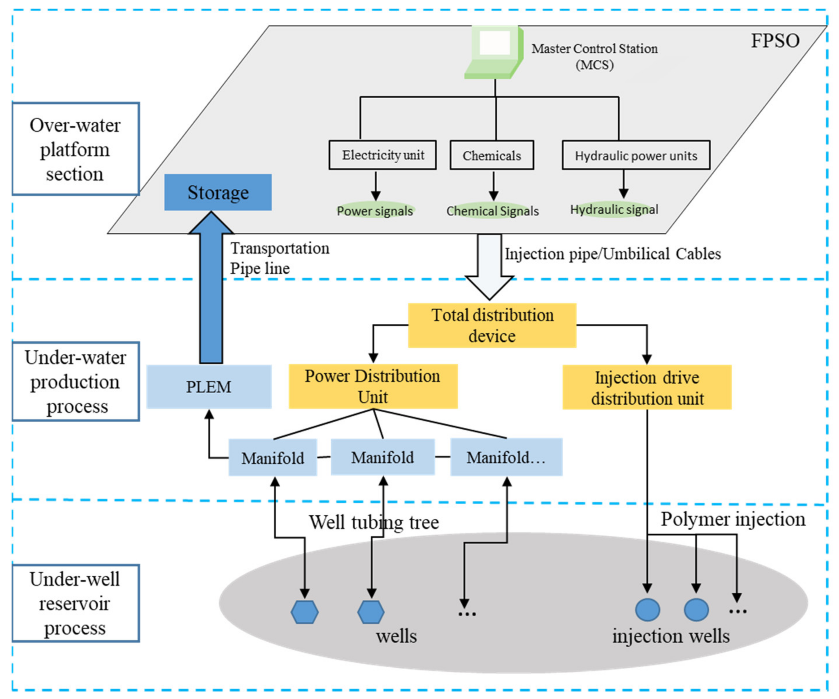
From the wells to the platform, the whole production process can generally be divided into three parts: the under-well reservoir process, the under-water production process and the over-water platform section (Figure 1).
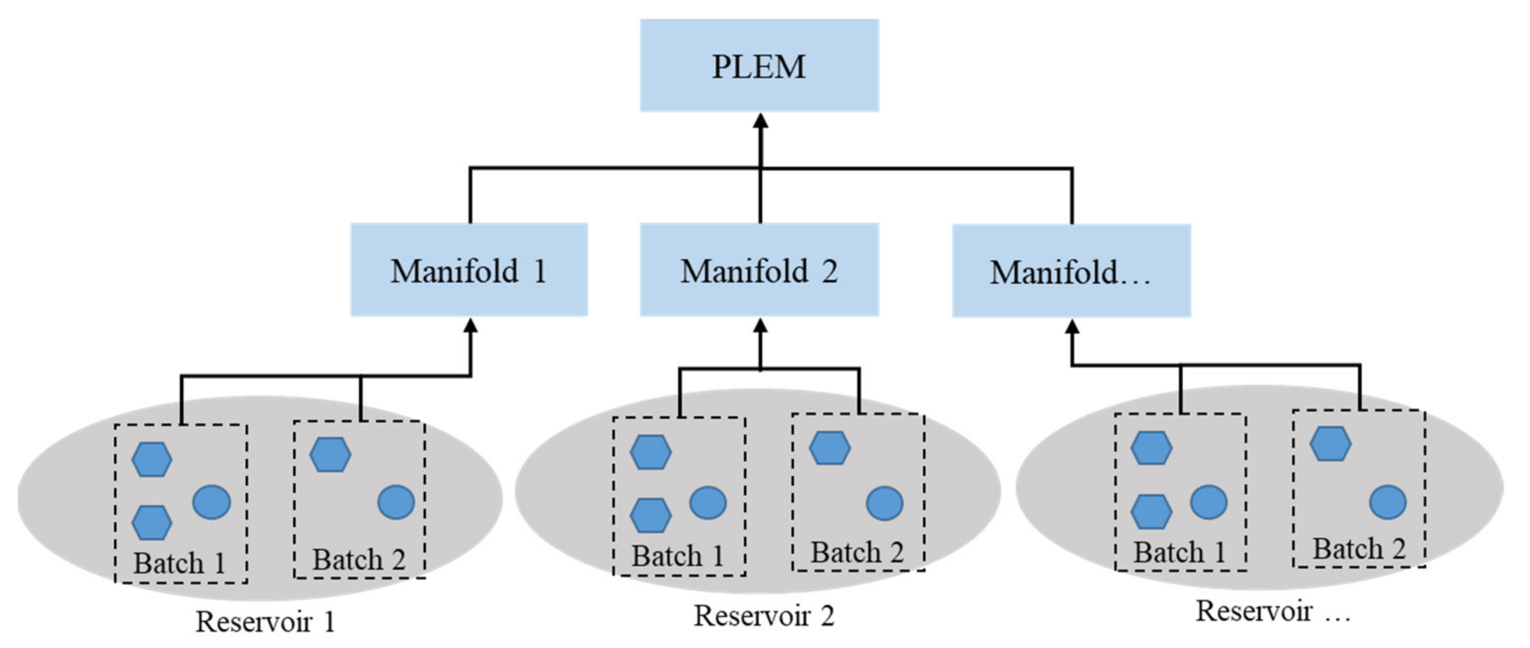
Wells are widely distributed in oilfield. Typically, an oilfield contains a lot of reservoirs, each of which in turn contains many wells. Wells can be divided into different batches of oil wells by the wells’ geological properties and physical characteristics, as shown in Figure 2. Wells belonging to the same batch interconnect with each other through a complex comprehensive pipeline network to convey liquid to manifold (i.e., PLEM in Figure 2). Wells in the same reservoir are grouped into one batch and normally share a surface equipment, usually named floating production, storage and offloading unit (FPSO). The whole oil and gas production process include five parts: optimization of oil well start-up and shutdown operation, optimization of electric submersible pump energy consumption, optimization of FPSO storage, optimization of polymer injection and flooding and flow safety guarantee. The key and difficult points of system integration modeling are:
- Optimize the capacity consumption of electric submersible pump (ESP) under changing flow conditions;
- Use the flow guarantee mechanism to balance the optimal operation scheme of oil wells and ensure the flow safety;
- Allocate the injection strategy of each well with a given amount of polymer;
- Integrate well and platform operations to separate or store oil/gas delivered to the platform.
Considered in terms of practical industrial problems, the following issues need to be considered in planning modelling:
- To facilitate modeling, the entire offshore oil and gas production process is regarded as a continuous production process, and all production-related variables can be connected through time;
- The whole oilfield is divided into several blocks according to geographical location, product characteristics and other conditions, and the modeling is optimized according to the blocks;
- To ensure smooth production, start-up and shutdown operation of each underwater well shall be considered;
- In order to ensure safe production, considering the protective effect of flow assurance guarantee on the production process, the cost of single wax removal is considered.
Taking the process flow diagram of offshore oil and gas production process shown in Figure 2 as the research object, the system integration modeling is carried out in consideration of equipment optimization at the operational layer and flow safety assurance technology. Several assumptions are made in this study as follows:
- The production wells are separated and totally independent of each other. It is natural because each well has its own independent reservoir.
- During the middle and later periods of oilfield development, artificial lift technology and polymer flooding is indispensable;
- All the electric submersible pumps have the same working characteristic curve;
- Geological properties characterizing the well are available;
- In the absence of polymerization flooding, oil recovery rate remains the lowest;
- The location of easily blocked pipeline section is known;
- Ignore the pressure change in the pipe.
With the above assumptions, the model relies on the following given information:
- A planning horizon and planning period;
- Production tasks for each batch of oil wells along the planning horizon;
- Working load range of oil production wells;
- A set of storage bins, their minimum and maximum stock and initial inventories;
- The penalty of switching operations and stock out;
- A set of cost coefficient and model parameters.
The decision variables are:
- The production rate and operating state of each oil well in each time period;
- The detailed delivery quantity in each oil batch in each time period;
- The injection displacement volume of each well;
- Diesel fuel consumption within each planning period;
- The wax removal cycle of each well.
The integrated planning model defined as a multi-period MINLP has been developed in our previous report. To improve readability, the original model is detailed as follows.
Mathematically, the objective function is given as follows:
The objective described in Equation (1) aims at minimizing the overall cost (Z), which includes the oil well open-close switching penalty(Z1), energy consumption (Z2), oil inventory (Z3), and chemicals cost (Z4), wax removal cost (Z5) and the costs of stock out penalty (Z6). Constraints related to Z1 to Z6 are shown in Equations (2)–(48). The specific meaning of each equation has been specified in our published articles 18.
2.2. Problem Statement
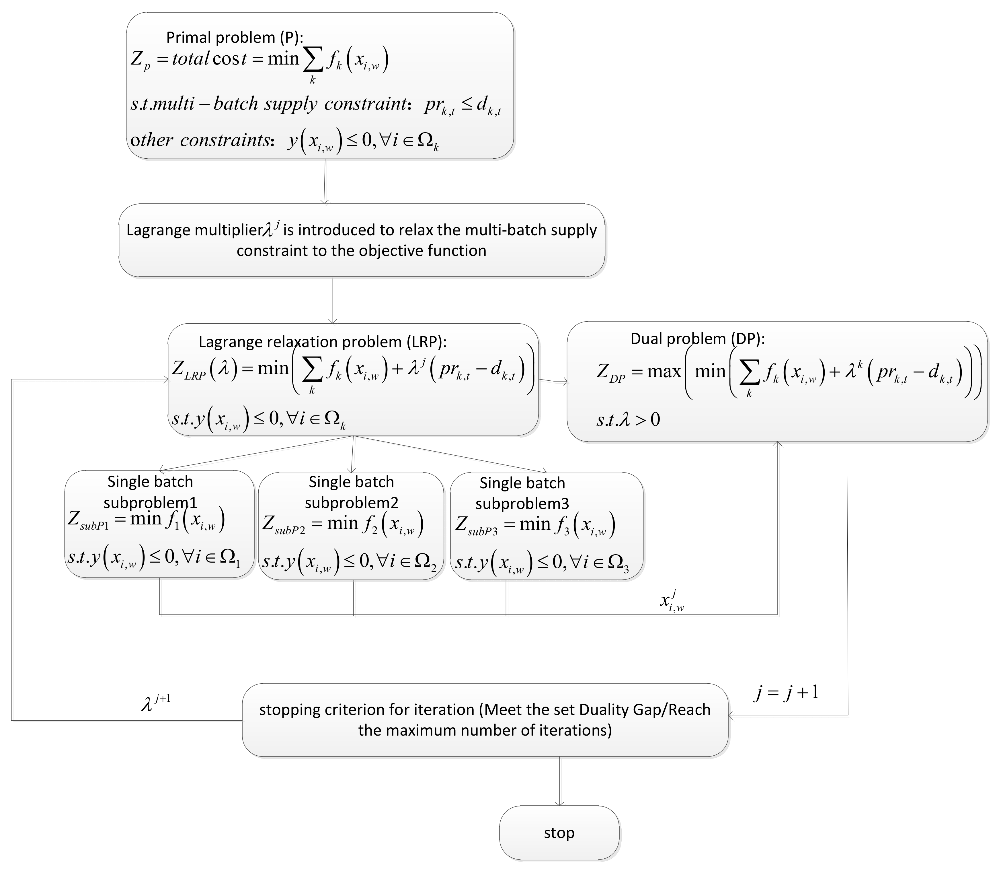
The MINLP model is theoretically difficult to solve especially for the industrial case. In addition, long-period planning time horizon and a large amount of parallel equipment will result in a large number of continuous and discrete variables, leading to the difficulty of low solving efficiency. In order to further improve the solving efficiency and meet the actual industrial production requirements, a batch decomposition algorithm based on Lagrange relaxation (LR) is proposed in this paper to solve the MINLP model. Problems that can use LR algorithm generally have the following characteristics: the objective function is differentiable with respect to the decision variables and constraints and there is a strong coupling between the constraints. The idea of LR [34] is to introduce Lagrange multipliers, which combine coupling constraints with multipliers as a form of relaxation into the original objective function as a penalty term. The original problem is transformed into a relaxation problem without the coupling constraint, thus decomposing the relaxation problem into sub-problems with multiple decision variables, fewer constraints and that is easier to solve. The batch decomposition algorithm based on Lagrange relaxation proposed in this paper decomposes the simultaneous optimization of multi-batch well packs into the optimization of single-batch well packs. Lagrange multipliers are introduced to relax the coupling constraints of multi-batch well packs, and dual problems are constructed to form cyclic iterations. Lagrange multiplier is introduced to relax the multi-batch coupling constraint to the objective function, the single-batch subproblem is obtained, and the solution is taken as the upper bound of the original problem. Secondly, the Lagrange dual problem is constructed, and the solution of the dual problem is taken as the lower bound of the original problem. The quality of the solution is judged by the duality gap between the upper and lower bounds, and the iterative algorithm is realized by continuously updating the multiplier by the step-by-step gradient method, which solves the large-scale problem caused by multi-batch coupling and simultaneous solution and greatly accelerates the solution speed.
2.3. LR Algorithm Implementation
The main steps of solving the planning problem are as follows: The multi-batch supply constraints as coupling constraints, i.e., Equation (48), are relaxed and embedded as a penalty term multiplied by Lagrange multipliers in the objective function, leading to a relaxation of the original problem. The relaxation problem can be decomposed into several single independent batches of sub-problems that are easier to solve. The Lagrange dual problem is represented by the LR method trying to maximize the dual objective function based on the duality theory. The solution of the dual problem is the lower bound of the original problem. Then, a feasible solution is constructed according to the solutions of the subproblems as the upper bound of the original problem. The goodness of the solution is judged by the duality gap of the upper and lower bounds. The sub gradient optimization method is used to update Lagrange multipliers. Until the iteration termination condition is met, the algorithm is terminated. The block diagram of LR algorithm is shown in Figure 3.
3. Multi-Well Batch Decomposition Algorithm
The wells in different blocks are divided into different well batches k. The production tasks of each well batch should meet the established annual production plan. Furthermore, each oil well batch relates to the others through underwater pipelines, with coupling constraints. Therefore, the multi-well batch coupling constraint is relaxed into the objective function of the original problem, and the relaxation problem is constructed to eliminate the coupling relationship between each well batch. At the same time, the relaxation problem is generally separable, which can be decomposed into sub-problems of each single well batch.
The objective function of the optimization problem is Equation (1), which means to find the minimum value of the total production cost.
3.1. Construction of Lagrange Relaxation LRP
Where the total cost is expressed as the superposition of costs of each link, as shown in Equation (49):
The original optimization problem satisfies the constraint conditions from Equations (2)–(48).
A set of Lagrange multiplier is introduced to relax the batch demand constraint (48) into the objective function to obtain the Lagrange relaxation problem (LRP), as shown in Equation (50):
where the batch demand constraint (49) can be converted into the form of Equation (51):
The objective function of the relaxation problem can be translated into Equation (52):
Similar terms in the relaxation problem are combined and converted into the form that can be decomposed into single-well batch sub-problems, as shown in Equation (53):
The relaxation problem satisfies the constraints of Equations (2)–(47).
Each term in the above equation can be derived from the well batch k. Therefore, given a set of values of Lagrange multiplier , the Lagrange relaxation problem for multiple well batches can be decomposed into a single well batch problem for each well in each well batch, as shown in Equation (54) below:
The single well batch subproblem satisfies the constraint conditions of Equations (2)–(47), and the final production target only needs to complete the annual planned production task of the corresponding well batch. The feasible solution obtained by solving the subproblem is regarded as the upper bound of the optimal solution of the original problem.
3.2. Construct Lagrange Duality Problem
The Lagrange relaxation problem is constructed to obtain the lower bound of the optimal solution of the original problem. However, the quality of the approximate optimal solution obtained by using this lower bound can hardly be satisfied. So, the Lagrange dual problem needs to be constructed to improve the quality of the lower bound and get a tighter bound.
Lagrange relaxation problem (LRP) is considered, as shown in Equation (55):
Equation (55) is the function of decision variables and , satisfying the constraint conditions Equations (2)–(47), with the purpose of obtaining the minimum cost of the objective function.
Then the dual problem can be expressed as the following Formula (56):
The above equation is the function of Lagrange multiplier . The fixed decision variable obtained from the relaxation problem is taken as the input of the dual problem, and Equation (57) is taken as the constraint condition of the dual problem. The maximum value in the minimum problem is obtained to provide a tighter lower bound.
3.3. Algorithm Iteration
In order to make the feasible solution obtained by the decomposition algorithm approach to the optimal solution of the original problem step by step, the Lagrange multipliers given at the beginning need to be updated iteratively. So, the upper and lower bounds provided by the dual problem and the relaxation subproblem are closer and tighter until the desired requirements of the decision maker are met.
The updating principle of Lagrange multiplier adopts sub gradient descent algorithm, as shown in Equation (58):
The is the step size of the iteration, and is the sub gradient of coupling constraint in the Lagrange relaxation problem, which can be expressed as Equation (59):
Step size can be defined as the following Equation (60) [35]:
In the formula, represents the best objective function value found until the step of iteration. The size of duality gap is taken as the judgment criterion. is the dual function value obtained in the iteration. is the given initial step size, which is generally between 0 and 2. When the duality gap is less than a given requirement or reaches a certain CPU time (number of iterations), the algorithm terminates. The duality gap can be expressed as Equation (61):
In Equation (61), represents the value of the objective function corresponding to the feasible solution of the subproblem, and represents the value of the objective function of the dual problem. All of the above symbols are detailed in Abbreviations.
4. Case Studies
This section may be divided by subheadings. It should provide a concise and precise description of the experimental results, their interpretation and the experimental conclusions that can be drawn. In order to compare with the solution results of ALPHAECP and verify the advantages of this algorithm in solving large-scale problems, four cases with different model sizes are given. Case 1 includes 1 oil well batch, 4 production wells and 12 planning cycles. Case 2 includes 2 well batches, 8 production wells and 12 planning cycles. Case 3 includes 3 oil well batches, 12 production wells and 12 planning cycles, the same as the case of published papers [18]. Case 4 includes 3 well batches, 12 production wells and 24 planning cycles. The crude oil requirement per well batch per month is given separately.
Given four cases, the model size gets progressively larger, with Case 2 having one more well lot than Case 1, Case 3 having one more well lot than Case 2 and Case 4 having one more planning cycle than Case 3. Case 1 is a single oil well batch problem, which is not applicable to the proposed batch decomposition algorithm. It is directly solved by ALPHAECP solver, and the results of Case 1 are used for comparison of other cases. Other cases are solved by the proposed algorithm respectively, and the results of the unique variables are compared to verify the solution effect of the algorithm on different scale problems.
4.1. Results Presentation
As shown in Table 1, Table 2, Table 3 and Table 4, the monthly plan arrangement of each batch of oil wells is given in the table. There are four wells in each batch. The effectiveness of the algorithm is verified by four examples.
These cases are computed by GAMS win32 24.0.2, and subproblems are solved by the solver of ALPHAECP in an Intel core i5-7500 CPU, 3.41 GHz machine with 8 GB of RAM. The model size statistics directly solved by ALPHAECP solver are shown in Table 5. Furthermore, the comparison results between multi-well batch model solution and LR algorithm are shown in Table 6.
4.1.1. Case 1: Single Oil Well Approval for 12 Months
The production schedule of Case 1 is shown in Table 1. Case 1 is a single-well batch problem, which can be solved directly by using the built-in ALPHAECP solver of GAMS. The solution gap is set at 1% and the CPU runtime is set at 100 s. The statistical results of Case 1 are shown in Table 5. The solution of single well batch is not applicable to the proposed batch decomposition algorithm, and the results are used to compare the results of the four cases to verify that large-scale problems are difficult to be solved directly. Thus, the validity of the algorithms in this chapter is highlighted by comparison.
4.1.2. Case 2: Two Oil Wells Were Approved for 12 Months
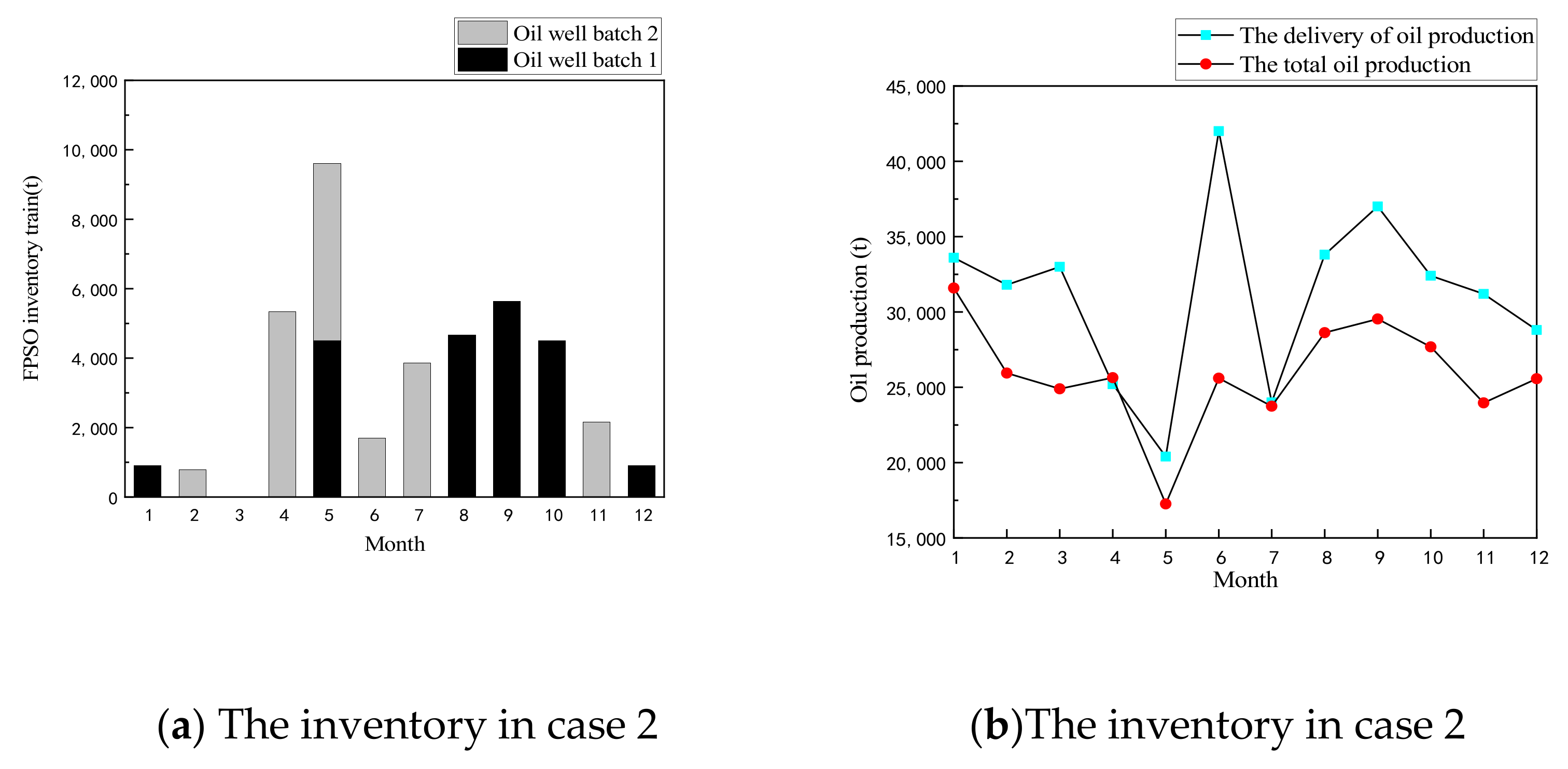
In Case 2, the size of the simulated reservoir can be divided into two different production blocks according to geographical conditions. Each block is the same batch of oil wells, and each block contains four production wells. Draw up the production plan for the next 12 months according to the market demand for different oil well batches. Table 2 shows the given monthly production schedule. The directly solved model size statistics are shown in Table 5. Then, the batch decomposition algorithm based on Lagrange relaxation proposed in this paper is used to decompose the two batches of the original problem into single batches to solve the sub-problems respectively. At the same time, LR dual problem is constructed to solve iteratively. Among them, the single-batch sub-problem and dual problem of Lagrange are solved directly by using the ALPHAECP solver built by GAMS. The comparison results of the two algorithms are shown in Table 6.
In Case 2, the total cost increased by 4.7% compared with the direct solution of LR algorithm. The solution time was significantly reduced by 43.7%.
Figure 4 shows the optimization solution results of Case 2. It can be seen from the figure that the output of each month plus the inventory of each month can meet the delivery requirements of that month. Therefore, there are no out-of-stock penalties occurring and the production planning requirements given in Case 2 can be met on time. So, applying the batch decomposition algorithm based on Lagrange relaxation to solve the planning optimization problem of the 12-month batch size of two oil wells, the market demand is satisfied, the process is not punished and the results are effective.
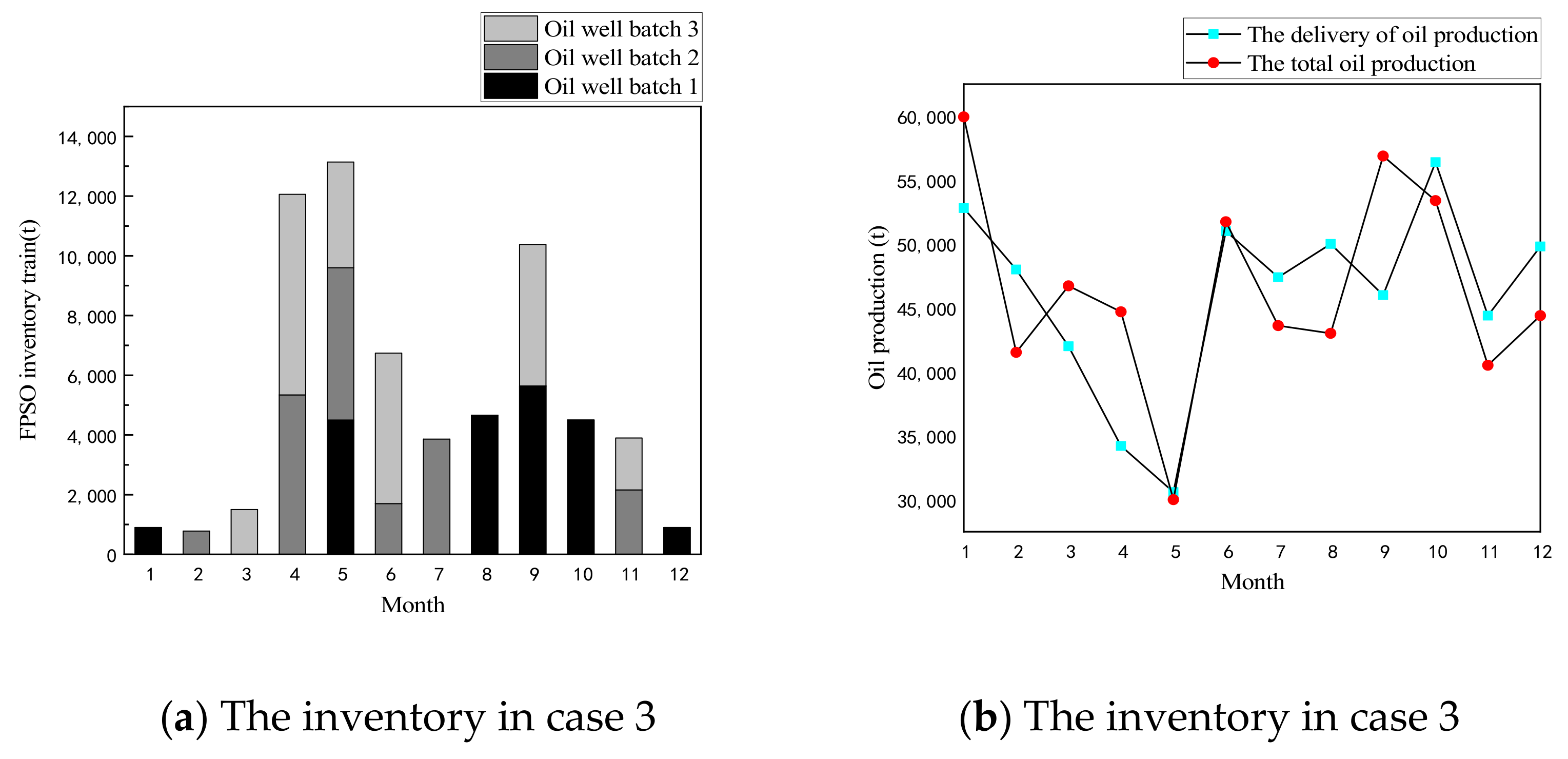
4.1.3. Case 3: Three Oil Wells Were Approved for 12 Months
In simulation case 3, the monthly production plan arrangement is shown in Table 3, the directly solved model size statistics are shown in Table 5 and the comparison of solution results of the two algorithms is shown in Table 6.
In Case 3, compared with the direct solution, the total cost of LR algorithm increased by 4.1%. The solution time was significantly reduced by 48.9%.
Figure 5 is the optimization results of Case 3. It can be seen from the figure that the output of each month plus the inventory of each month can meet the delivery requirements of that month. Therefore, there is no shortage penalty and the production plan requirements given in Case 3 can be completed on time. The results obtained by LR algorithm are effective and can meet the production requirements.
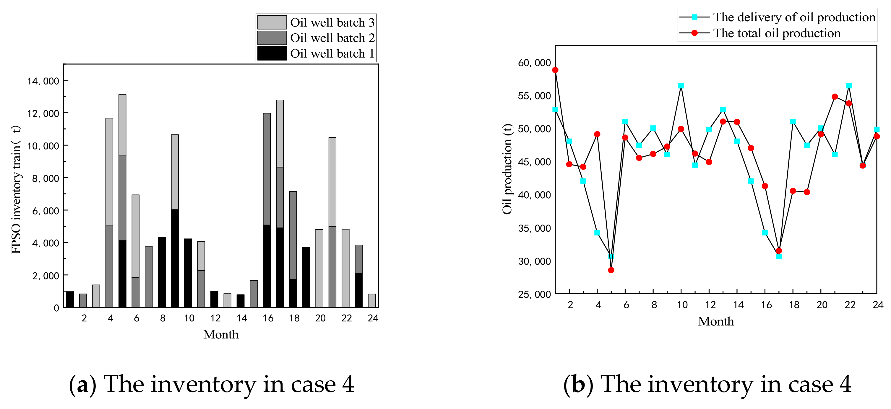
4.1.4. Case 4: Three Wells Group of 24 Months
In simulation case 4, the monthly production schedule arrangement is shown in Table 4, and the directly solved model size statistics are shown in Table 5, and the comparison of solution results of the two algorithms is shown in Table 6.
In Case 4, the total cost of solving LR algorithm increased by 3.8% compared with the direct solution. The solution time was significantly reduced by 61.6%.
Figure 6 shows the optimization solution results of Case 4, which is similar to Case 3. The result solved by LR algorithm can meet the production demand and be efficient.
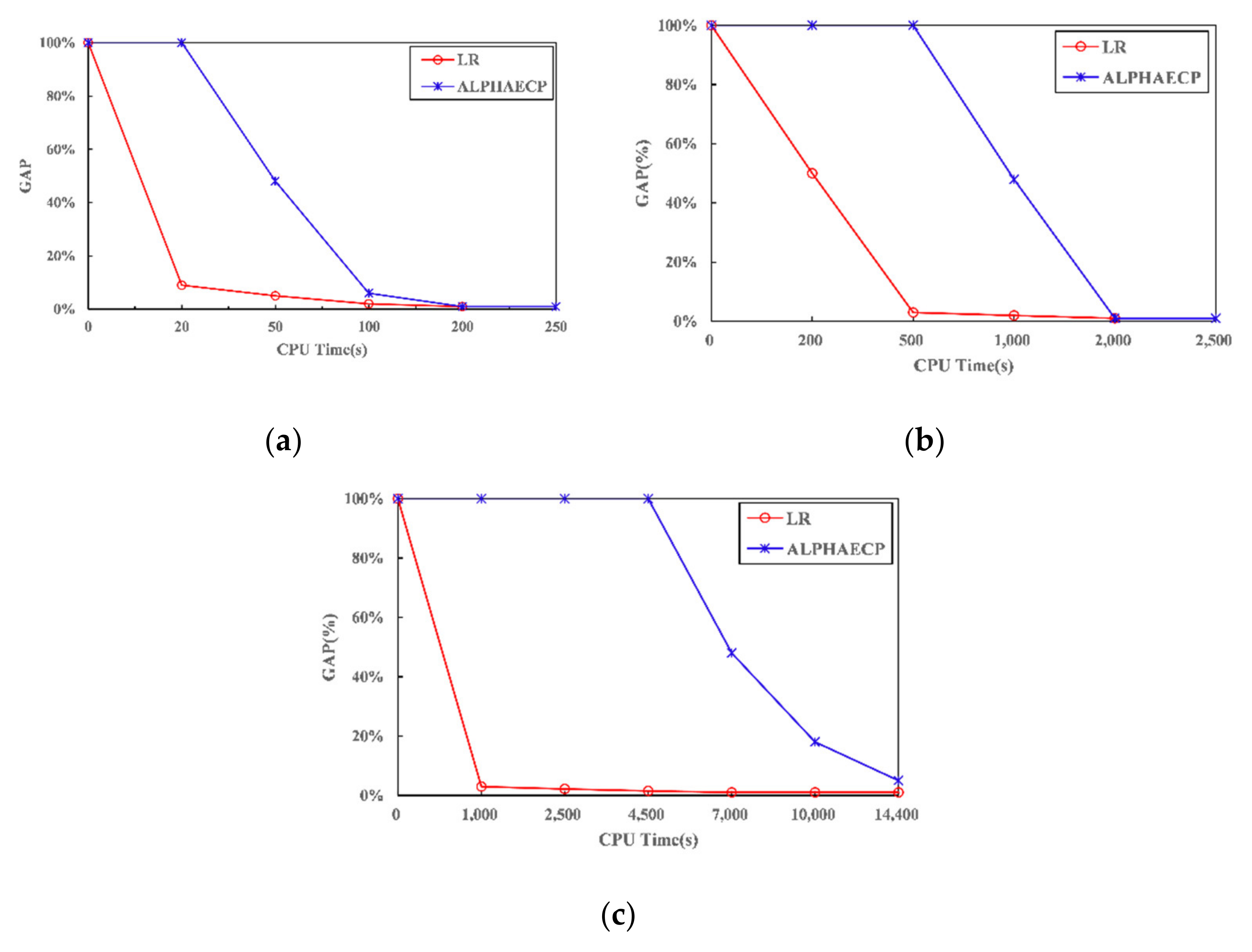
4.2. Results Presentation
The three control case groups with different sizes are compared, and the relationship between solving gaps and computing time is shown in Figure 7. The blue line is the trend of solving gaps directly solved by the ALPHAECP solver for MINLP model at a specified time and a specified suspension gap. Furthermore, the red line is the trend of solving gaps solved by LR algorithm for MINLP model. Obviously, in three cases of different sizes, the GAP value of the model solved by LR algorithm converges faster and can reach the required optimal GAP value in a shorter time.
The results of the four cases are compared together to verify the proposed batch decomposition algorithm for solving problems of different sizes.
The final algorithm comparison results of the four cases are shown in Table 6 above. By comparing the solution results of each case in the table above, the following conclusions can be drawn. In terms of CPU running time, the Lagrange relaxation-based batch decomposition algorithm proposed in this chapter on is at least 40% better than solving directly using the solver. Whether the problem of larger model size is caused by the increase in the number of devices or the increase in the planning period, the algorithm can significantly improve the solving efficiency, with the average solution time increasing by 49%. Moreover, the larger the problem size to be solved is, the greater the improvement of the solving efficiency will be. However, the final cost obtained by this algorithm is not better than that obtained by ALPHAECP. The reason may be that the solution obtained by this algorithm is only approximately the optimal solution. By relaxing the constraint into the objective function, the final optimization cost may become higher. However, as the problem gets bigger, the solutions get closer and closer. The results obtained by the proposed LR algorithm may not be globally optimal. The focus is to improve solving efficiency and to obtain the solution in reasonable time for industrial-scale problem.
5. Conclusions
The LR algorithm is used to decompose the large-scale MINLP problem, which is solved optimally for multiple well batches simultaneously, into subproblems that are solved independently for a single well batch. The multi-well batch coupling constraint is relaxed into the objective function by introducing Lagrange multipliers to remove the multi-batch coupling from the constraint. The relaxed problem is still of the MINLP model and is still more difficult to solve than LP or MILP models. However, the problem uses the LR algorithm to increase the feasible domain range and reduce the time required to search for a solution. Moreover, the resulted small scale MINLP model is not approximated and its result is more precise. The original problem is decomposed into several single batch sub-problems and the feasible solution obtained by solving the sub-problems is taken as the upper bound of the original problem. The Lagrange dual problem is also constructed as a lower bound on the original problem. The pairwise gap that exists between the upper and lower boundaries is used as a criterion for judging the quality of the feasible solution. The Lagrange multiplier is updated using the sub gradient method, which iteratively updates the upper and lower bounds continuously, making them tighter and tighter until the decision maker′s expectations are met. Four cases of different sizes are solved using the algorithm in this paper and solved directly by the solver through the case of a given four different scale, using this algorithm and direct solver. By analyzing and comparing the two results, the algorithm proposed in this paper can effectively improve the solving efficiency for tackling large-scale problems, with an average saving of 49% in solving time. Furthermore, the greater the scale of the problem, the better the results and the more instructive it is for practical industrial production.
Author Contributions
Conceptualization, X.G.; methodology, Y.W. and T.C.; software, Y.Z.; validation, X.G., Y.W. and X.Z.; formal analysis, T.C.; investigation, Y.Z.; resources, T.C.; data curation, Y.Z.; writing—original draft preparation, Y.Z.; writing—review and editing, X.G.; visualization, Y.Z.; supervision, X.G.; project administration, X.Z.; funding acquisition, X.G. All authors have read and agreed to the published version of the manuscript.
Funding
This work is supported by the National Natural Science Foundation of China (No. 21706282), National Key R&D Program of China (No. 2016YFC0303703), Science Foundation of China University of Petroleum, Beijing (No.s 2462020BJRC004, 2462020YXZZ023) and the UK BBSRC (BB/S020896/1).
Institutional Review Board Statement
Not applicable.
Informed Consent Statement
Not applicable.
Data Availability Statement
Not applicable.
Conflicts of Interest
The authors declare no conflict of interest.
Abbreviations
| ESP | electric submersible pump |
| FPSO | floating production storage and offloading |
| MILP | mixed integer linear programming |
| LP | linear programming |
| MINLP | mixed integer nonlinear programming |
| i | oil production well |
| k | well batch |
| t | time period |
| I | oil production wells |
| K | well batches |
| T | time period |
| convection heat transfer coefficient | |
| radius of the tubing | |
| the density of gas phase | |
| the density of liquid phase | |
| the liquid holdup | |
| the mass flow of the mixture | |
| the resistance coefficient | |
| thermal conductivity of insulation materials | |
| thickness of the insulation blanket | |
| thickness of the tubing | |
| valve opening change limit | |
| maximum wax deposit thickness | |
| , | coefficients of polymer flooding of well i |
| distribution density of wax | |
| maximum inventory capacity of oil | |
| minimum inventory capacity of oil | |
| temperature of flowing-out | |
| , | coefficients of pressure increase of well i |
| , | coefficients of pressure decrease of well i |
| , | coefficients of pressure variation equation which result from combinations |
| production demand of well batch k in time period t | |
| demand of production in period t | |
| pipe roughness of well batch k | |
| power generation efficiency of diesel generator set in platform | |
| up limit pressure of well i | |
| down limit pressure of well i | |
| inlet pressure | |
| maximum production rate of well i | |
| minimum production rate of well i | |
| cost of start-stop operation of unit i | |
| coefficient for electricity consumption of valve in well i | |
| length of pipeline segment | |
| 1 | the line angle |
| A | the pipeline cross-sectional area |
| TL | temperature of flowing-in |
| Ts | temperature of fluid at the fluid entry point |
| ρ | is fluid density |
| density of wax | |
| length of time period | |
| suitable upper limit | |
| length of planning horizons | |
| coefficient of inventory cost | |
| cost coefficient of polymer flooding | |
| punishment of delivery delay | |
| coefficient of wax removal cost | |
| initial bottom pressure for the well i | |
| initial inventory level for the oil batch k | |
| half of the radius of the annular region volume by uneven ups and downs. | |
| a set of Lagrange multiplier | |
| the step size of the iteration | |
| the sub gradient of coupling constraint | |
| the given initial step size | |
| the duality gap | |
| temperature inside the pipe | |
| recovery ratio differential of oil well i in period t | |
| initial inventory of well batch k | |
| inventory of well batch k in the time period t | |
| quality of the precipitated wax in pipeline of well batch k | |
| polymer flooding of well i in time period t | |
| heat accumulation | |
| heat flow in | |
| heat flow out | |
| heat transferred | |
| pressure differential in the well bore when the well i is shut in | |
| wax removal cycle of well batch k | |
| volume of the precipitated wax in pipeline of well batch k | |
| pressure differential in the well bore when the well i is producing | |
| 0–1 variable indicating whether the well bore pressure reaches the maximum allowable value in period t when well i is closed | |
| consumption of energy | |
| initial pressure of well i | |
| well bore pressure of well i at the end of period t | |
| well bore pressure of well i at the beginning of period t | |
| production supply of oil well batch k in the time period t | |
| production supply in period t | |
| wax deposit rate in pipeline of well batch k | |
| the occurrence of start–stop operation in equipment i during t week and t + 1 week. | |
| 0–1 variable denoting whether well i is working in the period t | |
| production rate of oil in well i in the period t | |
| difference in temperature between the pipeline product and the ambient temperature outside | |
| wax deposit thickness | |
| v | fluid velocity in pipeline |
| energy supply |
References
- Song, Q.; Huang, G.; Shi, X. Analysis on current situation of petroleum consumption and countermeasures of traditional petroleum enterprises in China. Petrochem. Technol. Appl. 2018, 36, 149–153. (In Chinese) [Google Scholar]
- Yin, S. The Global Distribution of Oil and Gas Resources in Deep Waters; China University of Petroleum (Beijing): Beijing, China, 2018. (In Chinese) [Google Scholar]
- Peng, D.; Pang, X.; Chen, C.; Shu, Y.; Ye, B.; Gan, Q.; Wu, C.; Huang, X. From shallow water shelf to deep water continental slope—A Study on the Deep water fan system in the South China Sea. Acta Sediba Sin. 2005, 1, 1–11. (In Chinese) [Google Scholar]
- Jiaxiong, H.; Bin, X.; Xiaobin, S.; Yongjian, Y.; Hailing, L.; Pin, Y. Prospect and progress for oil and gas in deep waters of the world, and the potential and prospect foreground for oil and gas in deep waters of the South China Sea. Nat. Gas Geosci. 2006, 17, 747–752. [Google Scholar]
- Xu, X. Entering the Deep Sea: The Hope of China’s Oil and Gas Development. In China Business News; Chinese Economy Management Science Magazine: Beijing, China, 2012. (In Chinese) [Google Scholar]
- Alessandro, S. Trends and determinants of energy innovations: Patents, environmental policies and oil prices. J. Econ. Policy Reform 2020, 23, 49–66. [Google Scholar]
- Grossmann, I.E.; Erdirik-Dogan, M. Planning Models for Parallel Batch Reactors with Sequence-Dependent Changeovers. AIChE J. 2007, 53, 2284–2300. [Google Scholar]
- Pinto, J.M.; Joly, M.; Moro, L.F.L. Planning and scheduling models for refinery operations. Comput. Chem. Eng. 2000, 24, 2259–2276. [Google Scholar] [CrossRef]
- Neiro, S.M.; Pinto, J.M. A general modeling framework for the operational planning of petroleum supply chains. Comput. Chem. Eng. 2004, 28, 871–896. [Google Scholar] [CrossRef] [Green Version]
- Palou-Rivera, I.; Alattas, A.M.; Grossmann, I.E. Integration of Nonlinear Crude Distillation Unit Models in Refinery Planning Optimization. Ind. Eng. Chem. Res. 2011, 50, 6860–6870. [Google Scholar]
- Joly, M.; Moro, L.F.L.; Pinto, J.M. Planning and scheduling for petroleum refineries using mathematical programming. Braz. J. Chem. Eng. 2002, 19, 207–228. [Google Scholar] [CrossRef] [Green Version]
- Gupta, V.; Grossmann, I.E. An Efficient Multiperiod MINLP Model for Optimal Planning of Offshore Oil and Gas Field Infrastructure. Ind. Eng. Chem. Res. 2012, 51, 6823–6840. [Google Scholar] [CrossRef] [Green Version]
- Gupta, V. A New MINLP Model for Optimal Planning of Offshore Oil and Gas Field Infrastructure with Production Sharing Agreements. In Proceedings of the Computing and Systems Technology Division Core Programming Topic at the 2011 AIChE Annual Meeting, Minneapolis, MN, USA, 20 October 2011; pp. 1001–1002. [Google Scholar]
- Aseeri, A.; Gorman, P.; Bagajewicz, M.J. Financial Risk Management in Offshore Oil Infrastructure Planning and Scheduling. Ind. Eng. Chem. Res. 2004, 43, 3063–3072. [Google Scholar] [CrossRef]
- Ortiz-Gomez, A.; Rico-Ramirez, V.; Hernandez-Castro, S. Mixed-integer multiperiod model for the planning of oilfield production. Comput. Chem. Eng. 2002, 26, 703–714. [Google Scholar] [CrossRef]
- Lu, Y.; Jin, Q. Research on Lean Production Planning and Control Model Based on MES System. Manag. Adm. 2017, 5, 92–95. (In Chinese) [Google Scholar]
- Saravanan, V.; Nallusamy, S.; Balaji, K. Lead time reduction through execution of lean tool for productivity enhancement in small scale industries. Int. J. Eng. Res. Afr. 2018, 34, 116–127. [Google Scholar] [CrossRef]
- Gao, X.Y. Offshore oil production planning optimization: An MINLP model considering well operation and flow assurance. Comput. Chem. Eng. 2020, 133, 106674. [Google Scholar] [CrossRef]
- Patil, B.V.; Nataraj, P.S.V. An Improved Bernstein Global Optimization Algorithm for MINLP Problems with Application in Process Industry. Math. Comput. Sci. 2014, 8, 357–377. [Google Scholar] [CrossRef]
- Mouret, S.; Grossmann, I.E.; Pestiaux, P. A new Lagrangian decomposition approach applied to the integration of refinery planning and crude-oil scheduling. Comput. Chem. Eng. 2011, 35, 2750–2766. [Google Scholar] [CrossRef]
- Ghaddar, B.; Naoum-Sawaya, J.; Kishimoto, A.; Taheri, N.; Eck, B. A Lagrangian decomposition approach for the pump scheduling problem in water networks. Eur. J. Oper. Res. 2015, 241, 490–501. [Google Scholar] [CrossRef]
- Costa, L.; Oliveira, P. Evolutionary algorithms approach to the solution of mixed integer non-linear programming problems. Comput. Chem. Eng. 2001, 25, 257–266. [Google Scholar] [CrossRef]
- Jaffal, Y.; Nasser, Y.; Corre, Y.; Lostanlen, Y. K-best branch and bound technique for the MINLP resource allocation in multi-user OFDM systems. In Proceedings of the 2015 IEEE 16th International Workshop on Signal Processing Advances in Wireless Communications (SPAWC), Stockholm, Sweden, 28 June–1 July 2015; pp. 161–165. [Google Scholar]
- Aras, Ö.; Bayramoğlu, M. A MINLP Study on Shell and Tube Heat Exchanger: Hybrid Branch and Bound/Meta-heuristics Approaches. Ind. Eng. Chem. Res. 2012, 51, 14158. [Google Scholar] [CrossRef]
- Bergamini, M.L.; Grossmann, I.; Scenna, N.; Aguirre, P. An improved piecewise outer-approximation algorithm for the global optimization of MINLP models involving concave and bilinear terms. Comput. Chem. Eng. 2008, 32, 477–493. [Google Scholar] [CrossRef]
- Luo, Y.; Yuan, X.; Liu, Y. An improved PSO algorithm for solving non-convex NLP/MINLP problems with equality constraints. Comput. Chem. Eng. 2007, 31, 153–162. [Google Scholar]
- Held, M.; Karp, R.M. The traveling-salesman problem and minimum spanning trees. Oper. Res. 1970, 18, 1138–1162. [Google Scholar] [CrossRef]
- Fisher, M.L. Optimal solution of scheduling problems using Lagrange multipliers: Part II. In Symposium on the Theory of Scheduling and Its Applications; Springer: Berlin/Heidelberg, Germany, 1973; pp. 294–318. [Google Scholar]
- Luh, P.B.; Hoitomt, D.J.; Max, E.; Pattipati, K.R. Schedule generation and reconfiguration for parallel machines[C]//1989 IEEE International Conference on Robotics and Automation. IEEE Comput. Soc. 1989, 1, 528–533. [Google Scholar]
- Luh, P.B.; Hoitomt, D.J. Scheduling of manufacturing systems using the Lagrangian relaxation technique. IEEE Trans. Autom. Control 1993, 38, 1066–1079. [Google Scholar] [CrossRef]
- Yu, D.; Luh, P.B.; Soorapanth, S. A new Lagrangian relaxation based method to improve schedule quality. In Proceedings of the Proceedings 2003 IEEE/RSJ International Conference on Intelligent Robots and Systems (IROS 2003) (Cat. No. 03CH37453), Las Vegas, NV, USA, 27–31 October 2003; Volume 3, pp. 2303–2308. [Google Scholar]
- Van den Heever, S.A.; Grossmann, I.E.; Vasantharajan, S.; Edwards, K. A Lagrangean decomposition heuristic for the design and planning of offshore hydrocarbon field infrastructures with complex economic objectives. Ind. Eng. Chem. Res. 2001, 40, 2857–2875. [Google Scholar] [CrossRef]
- Álvarez, J.D.; Redondo, J.L.; Camponogara, E.; Normey-Rico, J.; Berenguel, M.; Ortigosa, P.M. Optimizing building comfort temperature regulation via model predictive control. Energy Build. 2013, 57, 361–372. [Google Scholar] [CrossRef]
- Boyd, S.; Boyd, S.P.; Vandenberghe, L. Convex Optimization; Cambridge University Press: Cambridge, UK, 2004. [Google Scholar]
- Fisher, M.L. An applications oriented guide to Lagrangian relaxation. Interfaces 1985, 15, 10–21. [Google Scholar] [CrossRef]
Figure 1.
An integrated oil production system.

Figure 2.
Illustration of pipeline network and well batch in oilfield.

Figure 3.
LR algorithm block diagram.

Figure 4.
Results of Case 2.

Figure 5.
Results of Case 3.

Figure 6.
Results of Case 4.

Figure 7.
Relationship between optimum gap and computational time, (a) Case 1, (b) Case 2, (c) Case 3.
Figure 7.
Relationship between optimum gap and computational time, (a) Case 1, (b) Case 2, (c) Case 3.


Table 1.
Case 1.
| Well Batch | Monthly Demand of Production | |||||||||||
|---|---|---|---|---|---|---|---|---|---|---|---|---|
| 1 | 2 | 3 | 4 | 5 | 6 | 7 | 8 | 9 | 10 | 11 | 12 | |
| 1 | 12,600 | 15,000 | 15,000 | 16,200 | 9000 | 27,000 | 15,000 | 15,000 | 22,000 | 18,000 | 16,200 | 9000 |
Table 2.
Case 2.
| Well Batch | Monthly Demand of Production | |||||||||||
|---|---|---|---|---|---|---|---|---|---|---|---|---|
| 1 | 2 | 3 | 4 | 5 | 6 | 7 | 8 | 9 | 10 | 11 | 12 | |
| 1 | 12,600 | 15,000 | 15,000 | 16,200 | 9000 | 27,000 | 15,000 | 15,000 | 22,000 | 18,000 | 16,200 | 9000 |
| 2 | 21,000 | 16,800 | 18,000 | 9000 | 11,400 | 15,000 | 9000 | 18,800 | 15,000 | 14,400 | 15,000 | 19,800 |
Table 3.
Case 3.
| Well Batch | Monthly Demand of Production | |||||||||||
|---|---|---|---|---|---|---|---|---|---|---|---|---|
| 1 | 2 | 3 | 4 | 5 | 6 | 7 | 8 | 9 | 10 | 11 | 12 | |
| 1 | 12,600 | 15,000 | 15,000 | 16,200 | 9000 | 27,000 | 15,000 | 15,000 | 22,000 | 18,000 | 16,200 | 9000 |
| 2 | 21,000 | 16,800 | 18,000 | 9000 | 11,400 | 15,000 | 9000 | 18,800 | 15,000 | 14,400 | 15,000 | 19,800 |
| 3 | 19,200 | 16,200 | 9000 | 9000 | 10,200 | 9000 | 23,400 | 16,200 | 9000 | 24,000 | 13,200 | 21,000 |
Table 4.
Case 4.
| Well Batch | Monthly Demand of Production | |||||||||||
|---|---|---|---|---|---|---|---|---|---|---|---|---|
| 1 | 2 | 3 | 4 | 5 | 6 | 7 | 8 | 9 | 10 | 11 | 12 | |
| 1 | 12,600 | 15,000 | 15,000 | 16,200 | 9000 | 27,000 | 15,000 | 15,000 | 22,000 | 18,000 | 16,200 | 9000 |
| 2 | 21,000 | 16,800 | 18,000 | 9000 | 11,400 | 15,000 | 9000 | 18,800 | 15,000 | 14,400 | 15,000 | 19,800 |
| 3 | 19,200 | 16,200 | 9000 | 9000 | 10,200 | 9000 | 23,400 | 16,200 | 9000 | 24,000 | 13,200 | 21,000 |
| 13 | 14 | 15 | 16 | 17 | 18 | 19 | 20 | 21 | 22 | 23 | 24 | |
| 1 | 21,000 | 16,800 | 18,000 | 9000 | 11,400 | 15,000 | 9000 | 18,800 | 15,000 | 14,400 | 15,000 | 19,800 |
| 2 | 19,200 | 16,200 | 9000 | 9000 | 10,200 | 9000 | 23,400 | 16,200 | 9000 | 24,000 | 13,200 | 21,000 |
| 3 | 12,600 | 15,000 | 15,000 | 16,200 | 9000 | 27,000 | 15,000 | 15,000 | 22,000 | 18,000 | 16,200 | 9000 |
Table 5.
Directly solved model size statistics.
| Case | Formula for the Number | Number of Nonlinear Terms | Number of Discrete Variables | Number of Continuous Variables | Duality GAP (%) | CPU Run Time (S) |
|---|---|---|---|---|---|---|
| CASE 1 | 2219 | 180 | 768 | 1587 | 1 | 100 |
| CASE 2 | 4438 | 394 | 1536 | 3174 | 1 | 1000 |
| CASE 3 | 6656 | 591 | 2304 | 4760 | 1 | 7200 |
| CASE 4 | 13,312 | 1167 | 4608 | 9520 | 5 | 14,400 |
Table 6.
Comparison of algorithms.
| Case | Cost | Relative Value of Difference (%) | Duality GAP (%) | CPU TIME (S) | Relative Value of Difference (%) | |
|---|---|---|---|---|---|---|
| CASE 1 | ALPHAECP | 163,786,288 | 1 | 12.27 | ||
| LR | ||||||
| CASE 2 | ALPHAECP | 355,809,355 | 4.7 | 1 | 242.02 | 43.7 |
| LR | 372,569,324 | 0.98 | 136.25 | |||
| CASE 3 | ALPHAECP | 515,030,600 | 4.1 | 1 | 2515.13 | 48.9 |
| LR | 535,930,049 | 0.96 | 1283.64 | |||
| CASE 4 | ALPHAECP | 941,556,300 | 3.8 | 5 | 14,400 | 61.6 |
| LR | 978,023,560 | 0.72 | 5531.25 |
Publisher’s Note: MDPI stays neutral with regard to jurisdictional claims in published maps and institutional affiliations. |
© 2021 by the authors. Licensee MDPI, Basel, Switzerland. This article is an open access article distributed under the terms and conditions of the Creative Commons Attribution (CC BY) license (https://creativecommons.org/licenses/by/4.0/).
Share and Cite
MDPI and ACS Style
Gao, X.; Zhao, Y.; Wang, Y.; Zuo, X.; Chen, T. A Lagrange Relaxation Based Decomposition Algorithm for Large-Scale Offshore Oil Production Planning Optimization. Processes 2021, 9, 1257. https://0-doi-org.brum.beds.ac.uk/10.3390/pr9071257
AMA Style
Gao X, Zhao Y, Wang Y, Zuo X, Chen T. A Lagrange Relaxation Based Decomposition Algorithm for Large-Scale Offshore Oil Production Planning Optimization. Processes. 2021; 9(7):1257. https://0-doi-org.brum.beds.ac.uk/10.3390/pr9071257
Chicago/Turabian StyleGao, Xiaoyong, Yue Zhao, Yuhong Wang, Xin Zuo, and Tao Chen. 2021. "A Lagrange Relaxation Based Decomposition Algorithm for Large-Scale Offshore Oil Production Planning Optimization" Processes 9, no. 7: 1257. https://0-doi-org.brum.beds.ac.uk/10.3390/pr9071257
Note that from the first issue of 2016, this journal uses article numbers instead of page numbers. See further details here.