A Hybrid Intelligent Fault Diagnosis Strategy for Chemical Processes Based on Penalty Iterative Optimization

Abstract

Process fault is one of the main reasons that a system may appear unreliable, and it affects the safety of a system. The existence of different degrees of noise in the industry also makes it difficult to extract the effective features of the data for the fault diagnosis method based on deep learning. In order to solve the above problems, this paper improves the deep belief network (DBN) and iterates the optimal penalty term by introducing a penalty factor, avoiding the local optimal situation of a DBN and improving the accuracy of fault diagnosis in order to minimize the impact of noise while improving fault diagnosis and process safety. Using the adaptive noise reduction capability of an adaptive lifting wavelet (ALW), a practical chemical process fault diagnosis model (ALW-DBN) is finally proposed. Then, according to the Tennessee–Eastman (TE) benchmark test process, the ALW-DBN model is compared with other methods, showing that the fault diagnosis performance of the enhanced DBN combined with adaptive wavelet denoising has been significantly improved. In addition, the ALW-DBN shows better performance under the influence of different noise levels in the acid gas absorption process, which proves its high adaptability to different noise levels.

1. Introduction

With the advancement of industrial intelligence, modern industry has higher requirements for system reliability and safety, which enables the rapid development of real-time risk management methods for efficiently detecting faults that threaten system reliability and eliminating uncertain noise affecting system safety. Among them, the fault detection and diagnosis (FDD) methods in the risk method play a central role [1].

Research on FDD technology began in 1971 [2], and it is now under rapid development. FDD methods can be classified into three categories: quantitative model-based, qualitative model-based and process history-based methods [3,4,5]. Among these methods, quantitative process history-based methods or data-driven methods possess the greatest potential for application in chemical processes [6]. A branch of data-driven methods relies on statistical measures such as principal component analysis (PCA) [7,8,9], independent component analysis (ICA) [10,11,12] and partial least squares (PLS) [13,14,15] for feature extraction and dimensionality reduction. The advantage of these methods is that they can simplify the analysis of complex dimensional data to improve efficiency. Other pattern classification methods, such as the artificial neural network (ANN) [16,17,18] and support vector machine (SVM) [19,20,21,22], have low generalization error rates and simple training processes. In addition, in recent years, new models have been developed by combining different data-driven methods to achieve the desired results, such as ICA-PCA [23], PCA-XGBoost [24] and the PCA-adaptive neuro-fuzzy inference system [25]. With the popularization of information construction in industrial plants and the development of deep learning (DL) methods, the research of FDD has ushered in another climax, such as convolutional neural networks (CNNs) [26,27] and deep belief networks (DBNs) [28].

Among them, deep belief networks are widely used in many fields, such as handwritten digit classification and computer vision. In these areas, DBNs outperform traditional ANNs at extracting the characteristics of the input data because of their efficient unsupervised pretraining process. In recent years, the research on DBNs has been intensified in the fault diagnosis-related research of DBNs. For example, the extended DBN proposed by Wang et al. [29] is used for chemical process fault diagnosis, and the layer-by-layer enhancement strategy based on DBNs proposed by Yu et al. [30] is used for chemical process fault detection. Significant results have been achieved in the fault diagnosis of the chemical process, but there are still the following two problems. One is that the data in chemical production processes often contain much noise, and the quality of the data may affect the performance of the FDD model. If the FDD model is established on the original process data directly, the fault diagnosis rate (FDR) will be low, and the false positive rate (FPR) will be high. Typical noise reduction methods mainly include a mean filter, Wiener filter, median filter, wavelet transform and denoising autoencoder. The tuning parameters of the noise reduction autoencoder, which is mostly used for image noise reduction, are more complicated, and the calculation time is longer [31]. The mean filter and median filter use the average or median value of the data in the neighborhood as the value after noise reduction, which can lose local information [32,33]. Wiener filtering needs to know the statistical characteristics of signal waveforms and cannot process nonlinear data, which makes the noise reduction effect on the chemical data poor, but the wavelet transform has excellent time–frequency localization characteristics, excellent denoising performance and easy extraction of weak signals [34]. It has achieved satisfactory results when dealing with complex nonlinear problems [35,36,37]. The traditional threshold methods of lifting wavelets mainly include the hard and soft threshold methods [38]. The continuity of the soft threshold method is usually better than that of the hard threshold method. The processed wavelet coefficients always have constant errors, which will cause inevitable errors after wavelet reconstruction. Aiming at the shortcomings of the soft threshold method, an adaptive soft threshold method is proposed. The adaptive lifting wavelet (ALW) denoising process is performed by calculating the adaptive threshold that best matches the data and improves the accuracy of noise reduction. Another problem is that the traditional DBN is mainly used for face recognition [39], which has the problem of falling into local optimization. The optimal value is often not the global best, and thus the accuracy of the fault diagnosis is often low. Therefore, this research optimizes the traditional DBN structure and adds an automatic iterative penalty factor to the network structure so that the DBN can overcome local convergence and improve the accuracy of fault diagnosis. The combination of the above two methods solves the two main problems of FDDs. The original DBN method, the enhanced DBN method, and the ALW combined with an enhanced DBN (ALW-DBN) method are applied to the TE process. The advantages of the enhanced method compared with the original one and the high precision of the combined method are proven. The application in industrial processes shows that the ALW-DBN method has strong adaptability and stability for different levels of noise, effectively protecting the safety and reliability of the system in the industrial process.

The rest of this paper is organized as follows: Section 2 includes the basic ideas of the structure of the enhanced DBN, the training process, the ALW to denoise the input data and the full procedure of the ALW-DBN fault diagnosis model. In Section 3, the appropriate wavelet decomposition layer and threshold method are selected by applying different thresholds to the TE process and then applying ALW-DBN methods in the TE process to prove the advantages of the ALW-DBN. In Section 4, the ALW-DBN model is applied to an acid gas absorption process to determine the adaptability of this model under different noise conditions and the degree of diagnostic accuracy.

2. Methods

2.1. Enhanced Deep Belief Network (DBN)

The traditional DBN was proposed by Hinton [40], which consists of multiple restricted Boltzmann machines (RBMs) and a top-level back propagation neural network (BPNN).

2.1.1. Traditional DBN

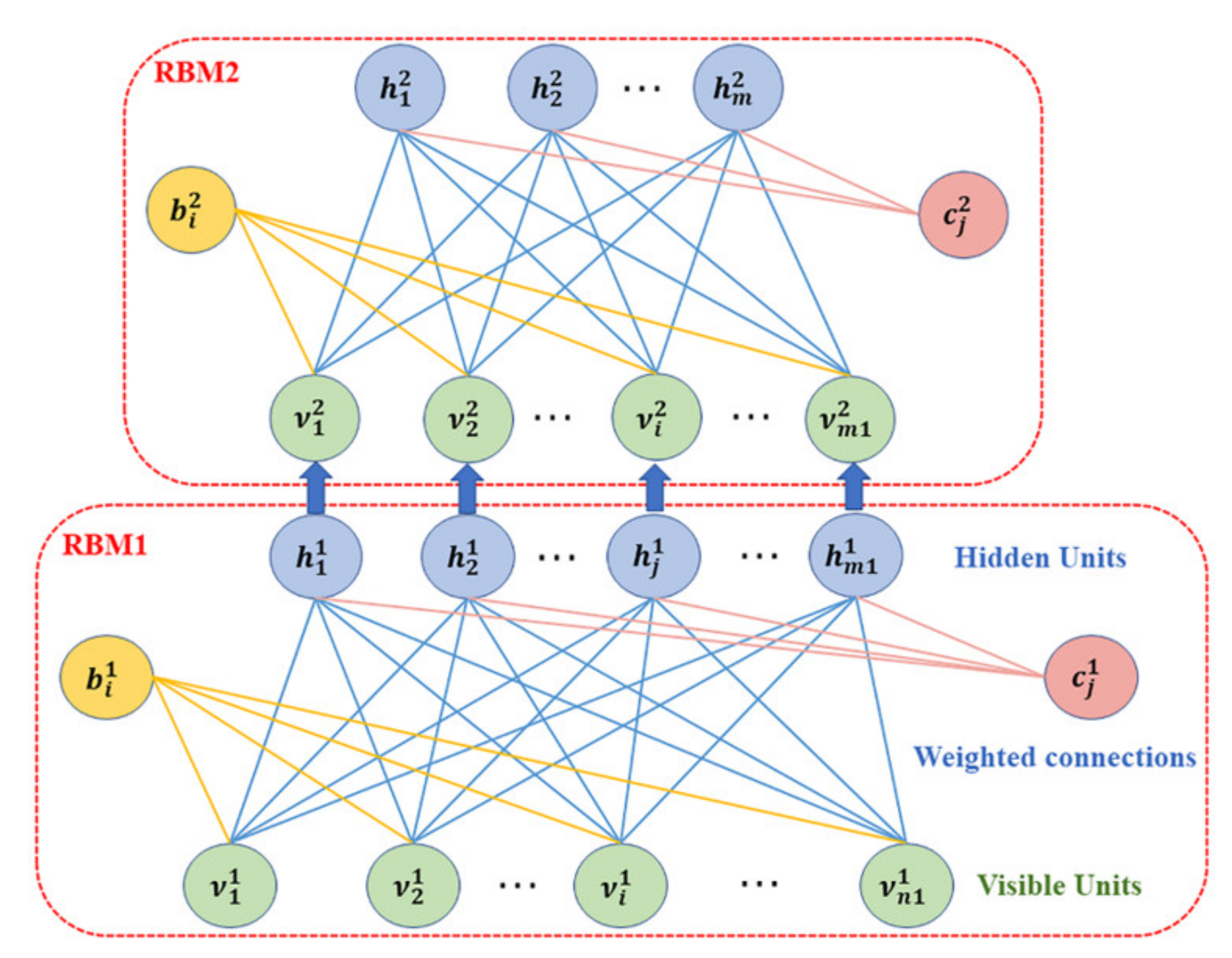
In the traditional DBN network, the RBM is a neural network with two layers of neurons, also known as the visible layer and the hidden layer. The visible layer consists of units that accept input data, whereas the hidden layer is separated from the input and contains units for feature extraction. The units within each layer are isolated from each other, but the units between the two layers are interconnected. A real number called the weight is associated with each interlayer connection. The structure of an RBM is illustrated in Figure 1.

For a given state $\left(v,h\right)$, an energy function can be defined as follows:

$$E_{\theta }\left(v,h\right)= -{\displaystyle \sum }_{i=1}^{n_v}{b}_i{v}_i-{\displaystyle \sum }_{j=1}^{n_h}{c}_j{h}_j-{\displaystyle \sum }_{i=1}^{n_v}{\displaystyle \sum }_{j=1}^{n_h}{h}_j{w}_{i,j}{v}_i$$

(1)

where $v_i$ and $h_j$ represent the binary state of the visible unit $i$ and the hidden unit j, respectively. $b_i$ and $c_j$ are their biases and $w_{ij}$ is the weight between units $i$ and j.

According to the energy function $E_{\theta }\left(v,h\right)$, the joint probability distribution of states $\left(v,h\right)$ can be derived as follows:

$$P_{\theta }\left(v,h\right)=\frac{1}{Z_{\theta }}{e}^{-E_{\theta }\left(v,h\right)}$$

(2)

where $Z_{\theta }$ is a normalization factor, expressed as

$$Z_{\theta }={\displaystyle \sum }_{v,h}{e}^{-E_{\theta }\left(v,h\right)}$$

(3)

In an RBM, the conditional probability of the hidden layer neurons being activated with respect to an input state is

$$P\left(h_j|v\right)=\sigma \left(b_j+{\displaystyle \sum }i{w}_{i,j}{v}_i\right)$$

(4)

Because an RBM is bidirectionally connected, the visible layer neurons can also be activated with conditional probability:

$$P\left(v_i|h\right)=\sigma \left(c_i+{\displaystyle \sum }j{w}_{i,j}{h}_j\right)$$

(5)

where $\sigma$ is the RELU function.

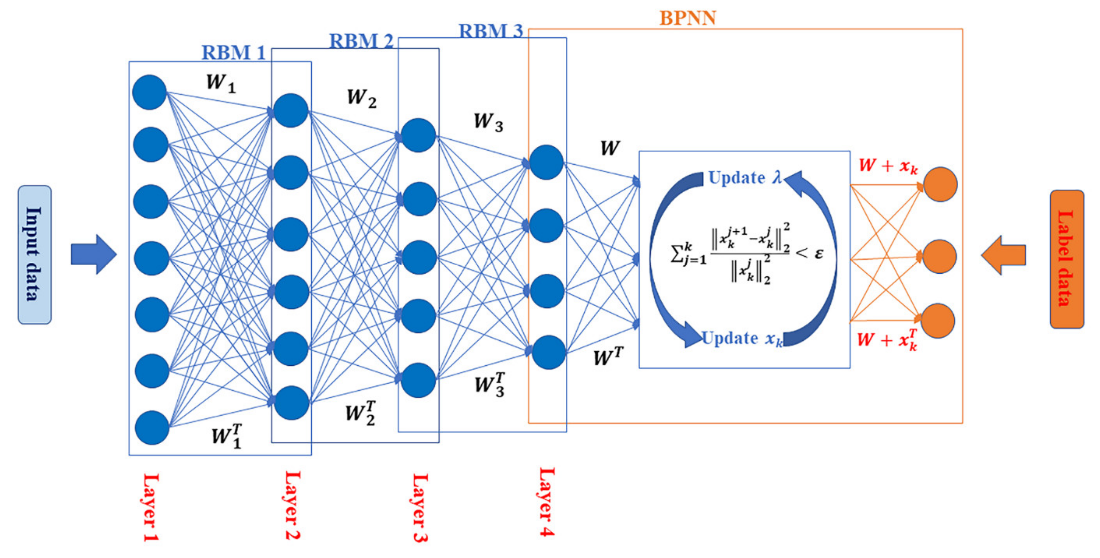
The proposed enhanced DBN is a deep neural network consisting of multiple RBMs as its bottom layers and an improved BPNN as its topmost layer. The structure of the enhanced DBN is shown in Figure 2. Layer 1 is the input layer, and layer 4 is the feature layer. Layers 1–4 can be considered three RBMs stacked together. The weights associated with each RBM in the form of matrices—that is, $W_1$, $W_2$, and $W_3$—are called detection weights. The transposes of these matrices, which are $W_1^T$, $W_2^T$, and $W_3^T$, are called generative weights. It forms a BPNN with the fourth layer and uses the label data of the training samples as the prediction target to fine-tune the entire network. In this layer, this paper adds a penalty factor to the formed BPNN to optimize the output result and update the manual optimization to automatic infinite optimization.

Training of an enhanced DBN involves two steps: pretraining and fine-tuning.

Pre-training is conducted to train each RBM sequentially through unsupervised learning, using the output of the previous RBM as the input of the next RBM. The standard method for training RBMs is the contrast divergence (CD) method proposed by Hinton [41].

After the training of all RBMs, the output of the last RBM is used as the input of the BPNN.

The fine-tuning of the DBN is achieved by supervised learning. Hinton proposed a wake-sleep algorithm [42], which suggests that in the wake state, the generation weights can be adjusted by the errors between the input data and the reconstruction data. However, the traditional DBN may cause errors to accumulate because of the standardized data matrix passing through the RBM layer by layer, eventually resulting in the appearance of a local optimum. The traditional DBN method manually adds the penalty number in the optimization process. This optimization method has an extremely low precision, and the adjustment process is significantly cumbersome. To avoid this situation, the traditional penalty terms are improved, and penalty factors are introduced to independently optimize the standardized matrix.

2.1.2. Penalty Factor

This paper introduces a penalty factor between the fourth and fifth layers of the DBN. The constrained optimization is converted to unlimited optimization to improve the diagnosis accuracy.

Consider these inequality constraints:

$$\underset{\left\{x_k\right\}}{\min }\{{\displaystyle \sum }_{j=1}^k\Vert {\sigma }_t[\left(\delta \left(t\right)+\frac{j}{\pi t}\right)\times x_{k}t]e^{-jt}{\Vert }_2^2\}$$

(6)

$$s.t{\displaystyle \sum }_{j=1}^k{x}_k=f$$

(7)

where $f$ is the input dataset and $x_k$ is the dataset decomposition. Therefore, the following augmented objective function can be constructed:

$$L\left(x_k,\mu \right):=r_k{\displaystyle \sum }_{j=1}^k\Vert {\sigma }_t[(\delta \left(t\right)+\frac{j}{\pi t})\times x_k\left(t\right)]e^{-jt}{\Vert }_2^2+\Vert f\left(t\right)-{\displaystyle \sum }_{j=1}^k{x}_k\left(t\right){\Vert }_2^2+\langle \mu \left(t\right)-{\displaystyle \sum }_{j=1}^k{x}_{k}t\rangle$$

(8)

where $r_k$ is the penalty factor and $\mu$ is the Lagrangian operator. The iterative update method is used to determine the saddle point of the Lagrangian expression, which is the optimal solution of the model. The optimization steps are as follows:

• The penalty factor is introduced by the DBN standardized dataset.
• Initialize the data $x_k^1$ and Lagrange operator ${\lambda }^1$.
• The initial point is iterated, and $x_k^{j+1}$ is updated as shown in Equation (9):

  $$x_k^{j+1}=argmin\{r_k^j\Vert {\sigma }_t\left[\left(\delta \left(t\right)+\frac{j}{\pi t}\right)\times x_k\left(t\right)\right]e^{-jt}{\Vert }_2^2+\Vert f-{\displaystyle \sum }_{j=1}^k{x}_k\left(t\right)+\frac{\lambda \left(t\right)}{2}{\Vert }_2^2\}$$

  (9)
• After updating $x$, update the Lagrangian operator $\lambda$ as shown in Equation (10):

  $${\lambda }^{j+1}={\lambda }^n+(x\left(t\right)-{\displaystyle \sum }_{j=1}^k{x}_k^j)$$

  (10)
• Equation (11) is used to determine whether the current iteration result meets the set error requirement. If the error requirement is not met, return to step 3 to continue the next iteration. If the error requirement is met, the current optimal penalty coefficient $r$ is obtained, and the DBN is input to reduce the cumulative error generated by each layer of RBM training:

  $${\displaystyle \sum }_{j=1}^k\frac{\Vert x_k^{j+1}-x_k^j{\Vert }_2^2}{\Vert x_k^j{\Vert }_2^2}<\epsilon$$

  (11)

The method to solve the optimal penalty parameter is iterative convergence (i.e., to determine whether the optimal value $x_k^j$ is reached through the result of each iteration). The optimal penalty item of the training dataset is matched to achieve the purpose of DBN training optimization.

Compared with the traditional DBN method of manually setting penalty items, the enhanced DBN method performs iterative calculations on the entire standardized dataset to obtain the optimal penalty item of the current dataset, and it has stronger adaptability to different data sets. The cumulative error generated by each layer of the RBM of the enhanced DBN network is minimized. The generalization of the final training process is reduced, and the training error is smaller. In comparison with traditional manual multiple adjustment training, this method is more accurate and convenient.

2.2. Adaptive Lifting Wavelet Method

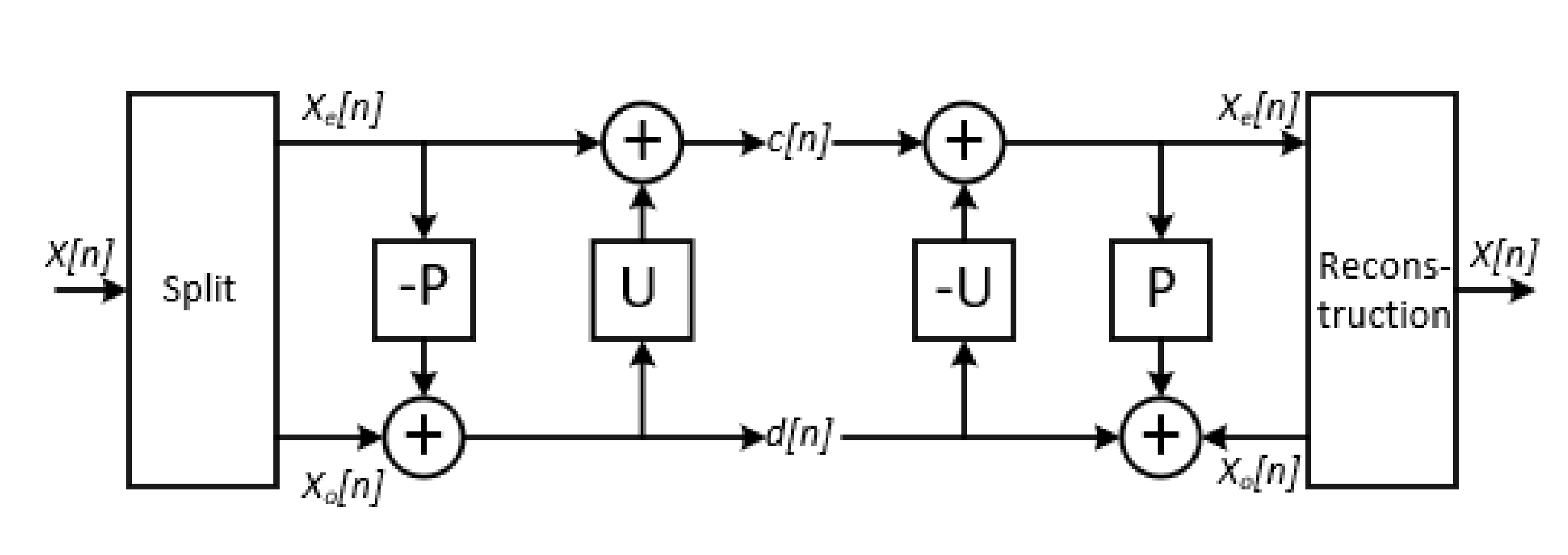
Modern industrial process data are often accompanied by noise interference, which affects process fault diagnosis. Aiming at the noise of the chemical process data in this study, the original lifting wavelet (LW) soft threshold method proposed by Wim Sweldens [38,43] is enhanced, and an ALW based on the adaptive soft threshold method is proposed. The ALW transformation consists of three steps: splitting, prediction and updating.

As shown in Figure 3, $P$ is the prediction operator, $U$ is the updating operator, $c\left[n\right]$ is the lifted low-frequency coefficient, $d\left[n\right]$ is the lifted high-frequency coefficient and $X_e\left[n\right]$ and $X_o\left[n\right]$ are the even and odd items of sampling, respectively.

(1) Splitting

The input signal $X\left[n\right]$ is decomposed into an even order sample $X_e\left[n\right]$ and an odd order sample $X_o\left[n\right]$. The decomposition effect of this step is proportional to the correlation between $X_e\left[n\right]$ and $X_o\left[n\right]$:

$$split \left(X\left[n\right]\right)=\left(X_e\left[n\right], X_o\left[n\right]\right)$$

(12)

(2) Prediction

Owing to the correlation between $X_e\left[n\right]$ and $X_o\left[n\right]$, $X_o\left[n\right]$ can be predicted by $X_e\left[n\right]$, and the prediction error is

$$X_{error}\left[n\right]=X_o\left[n\right]-P\left(X_e\left[n\right]\right)$$

(13)

where $X_{error}\left[n\right]$ is the high-frequency coefficient $d\left[n\right]$ of $X\left[n\right]$. This process is reversible. Similarly, $X_e\left[n\right]$ can be predicted based on $X_o\left[n\right]$.

(3) Updating

The updating process is conducted to adjust $X_e\left[n\right]$ according to $d\left[n\right]$ such that it contains only low-frequency components, denoted by $c\left[n\right]$:

$$c\left[n\right]=X_e\left[n\right]+U \left(d\left[n\right]\right)$$

(14)

Multi-level decomposition of the original signal can be obtained after several iterations of the original input signal using Equations (12)–(14).

Among them, the wavelet decomposition layer selection uses the $wavecode()$ function in MATLAB for decomposition, and the signal-to-noise ratio (SNR) is used to measure the pros and cons of the selected wavelet decomposition layer. The calculation equation of the SNR is as follows:

$$SNR=10log\left[\frac{{{\displaystyle \sum }}_{n}x{\left(n\right)}^2}{{{\displaystyle \sum }}_n{\left[x \left(n\right)-x^{\prime } \left(n\right)\right]}^2}\right]$$

(15)

where $x \left(n\right)$ is the original signal, $x^{\prime } \left(n\right)$ is the signal after noise reduction and $n$ is the signal length.

Traditional LW noise reduction methods include the hard and soft threshold methods, which show different effects in the noise reduction of data. The specific calculation is presented in Equations (16) and (17):

$$W_h=\left\{\begin{array}{c}w,\left|w\right|\ge T\\ 0,\left|w\right|<T\end{array}\right.$$

(16)

$$W_s=\left\{\begin{array}{cc}sgn\left(w\right)\left(\left|w\right|-T\right)\hfill & ,\left|w\right|\ge T\hfill \\ 0& ,\left|w\right|<T\hfill \end{array}\right.$$

(17)

where $W_h$ and $W_s$ represent the hard and soft threshold functions, respectively, and $w$ is the wavelet coefficient. The equation of the threshold $T$ is

$$T=\sigma \sqrt{2l{n}^{\left(N\right)}}$$

(18)

$$\sigma =\frac{1}{0.67Med\left(\left|x\right|\right)}$$

(19)

where $\sigma$ is the noise standard deviation and Med is the median function.

On the basis of the soft threshold function, after improving it, a new threshold function, namely the adaptive soft threshold, is obtained, which is expressed in Equation (20):

$$W_{ast.new}=\left\{\begin{array}{c}\omega +T-\frac{T}{2k+1}, \omega <-T\\ \frac{1}{\left(2k+1\right)T^{2k}}{\omega }^{2k+1},\left|\omega \right|<T\\ \omega -T+\frac{T}{2k+1},\omega >T\end{array}\right.$$

(20)

where $k$ is the adaptive coefficient. The expression is $k=1-e^{-\alpha {\left(\left|\omega \right|-T\right)}^2}$, and $\alpha$ is a positive number. The threshold obtained by the threshold estimation algorithm of Equations (18) and (19) is a fixed value. Using this threshold to process the wavelet coefficients produces the phenomenon of “over-killing”, which causes greater distortion when reconstructing the speech signal. Therefore, the use of traditional thresholds for wavelet coefficients under all decomposition scales filter out excessive useful signals and cause signal distortion. In view of the above analysis, this study adopts an adaptive threshold to process wavelet coefficients obtained under different decomposition scales.

After wavelet decomposition, the calculation of the noise standard deviation ${\delta }_j$ of the $j$th layer wavelet coefficients is expressed in Equation (21):

$${\delta }_j=\sqrt{\frac{1}{N_j}{\displaystyle \sum }_{k=0}^{N-1}{\left(W_k-\overline{W}\right)}^2}$$

(21)

where $N_j$ represents the number of wavelet coefficients of the $j$th layer, $W_k$ represents the wavelet coefficients of the $j$th layer and $\overline{W}$ represents the mean value of the wavelet coefficients of the $j$th layer.

When processing the wavelet coefficients of the $j$th layer, the threshold is set to $T_j$, and the calculation is as shown in Equation (22):

$$T_j=\frac{{\delta }_j\sqrt{2log{N}_j}}{log\left(j+1\right)}$$

(22)

where ${\delta }_j$ represents the standard deviation of the wavelet coefficient noise of the $j$th layer and $N_j$ represents the number of wavelet coefficients of the $j$th layer.

To determine the effect of adaptive soft threshold noise reduction, we used the root mean square error (RMSE) of the original signal and the denoised signal to measure the advantage of the adaptive soft threshold method. The equation is as follows:

$$RMSE=\sqrt[n]{\frac{1}{n}}{\displaystyle \sum }_n{\left[x \left(n\right)-x^{\prime } \left(n\right)\right]}^2$$

(23)

where $x \left(n\right)$ is the speech signal without noise and $x^{,} \left(n\right)$ is the speech signal after the denoising process. In general, the smaller the RMSE, the closer the denoised speech signal is to the original pure speech signal, indicating that the current algorithm has a better denoising effect. When selecting different adaptive wavelet coefficients $k$ and calculating the corresponding RMSE value, it can be observed that the smaller the RMSE value, the closer the corresponding $k$ value is to the optimal adaptive coefficient.

2.3. Fault Diagnosis Model

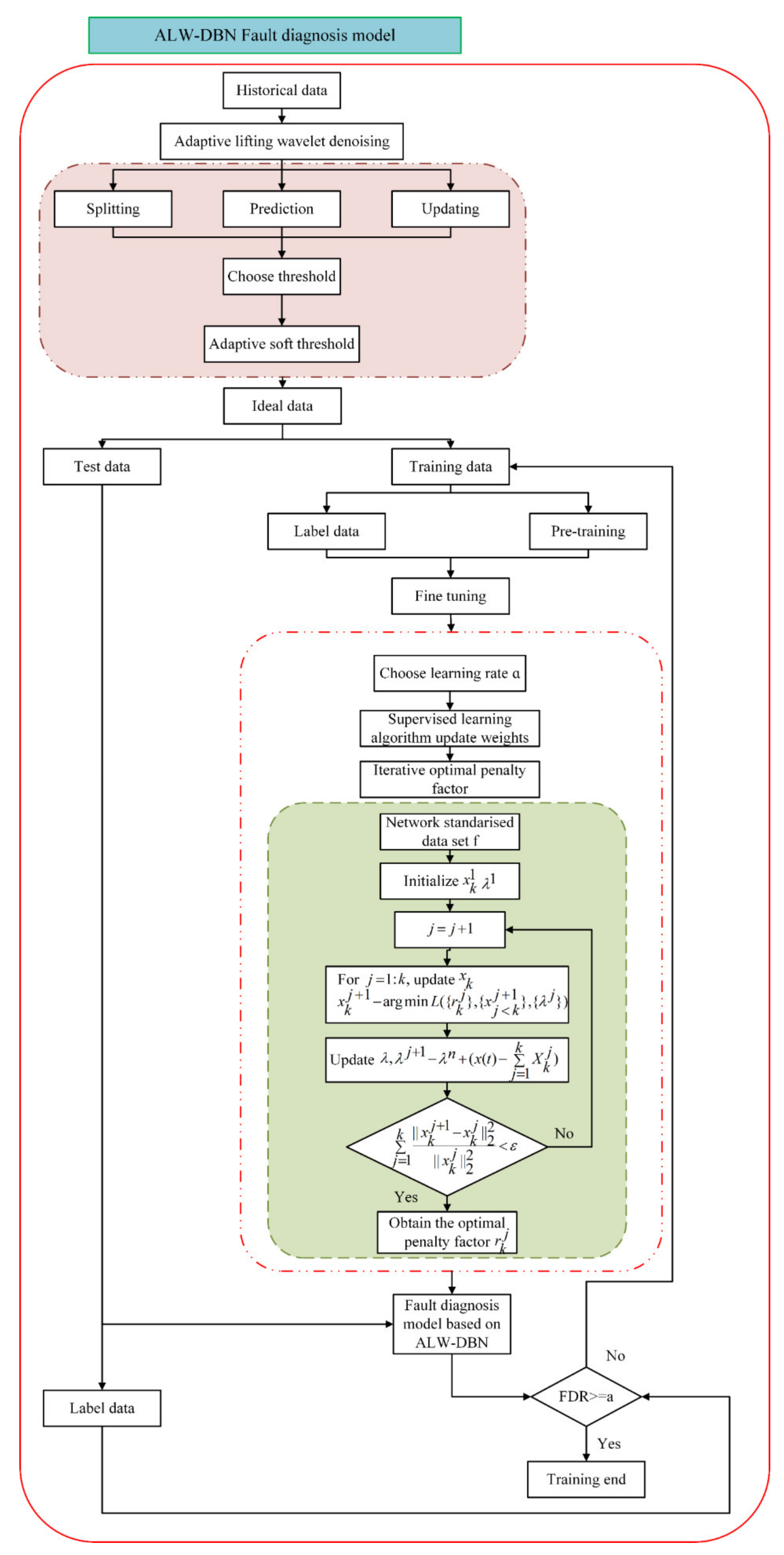
We propose a fault diagnosis model based on ALW-DBN for chemical processes. The framework of our model is illustrated in Figure 4.

First, the process data were upgraded by an adaptive wavelet transform, and the adaptive soft threshold method was used to reduce the noise after the wavelet lifting splitting, prediction, and update stages. Then, the ideal data were divided into a training set and test set according to the ratio of 4:1. The unlabeled data samples in the training set were pretrained using a layer-by-layer unsupervised algorithm. Pretraining was divided into two stages. The first stage included 100 iterations of pretraining with a momentum parameter of 0.5 and then 200 iterations of pretraining with a momentum parameter of 0.9. In the pretraining stage, the number of updated data samples in each batch was subject to actual process data samples. The model consisted of five RBM layers. After each RBM was fully trained, the entire network model was fine-tuned. In the fine-tuning stage, the learning rate $\alpha$ was determined, and then the weights $W_1,W_2,W_3,W_1^T, W_2^T,W_3^T$ were adjusted and updated by the wake-up sleep algorithm of supervised learning. At this time, local optimization may have occurred in the model, and hence, a penalty factor $r$ was added to optimize the penalty term of the model. We used penalty function for iterative optimization and iterated on the standardized network data completed by the pretraining to obtain the best penalty term $r_k^j$ for the training data set, correct the BPNN weights and reduce the accumulation of errors caused by multi-layer DBN training. After completion of the fine-tuning stage, the label data generated by the training set and the test set were input into the ALW-DBN diagnosis model. Finally, we determined whether the FDR reached the set standard $a.$ If not, a return to the retraining step was necessary.

3. Case Study of the Tennessee–Eastman Process

3.1. Tennessee–Eastman Process Description

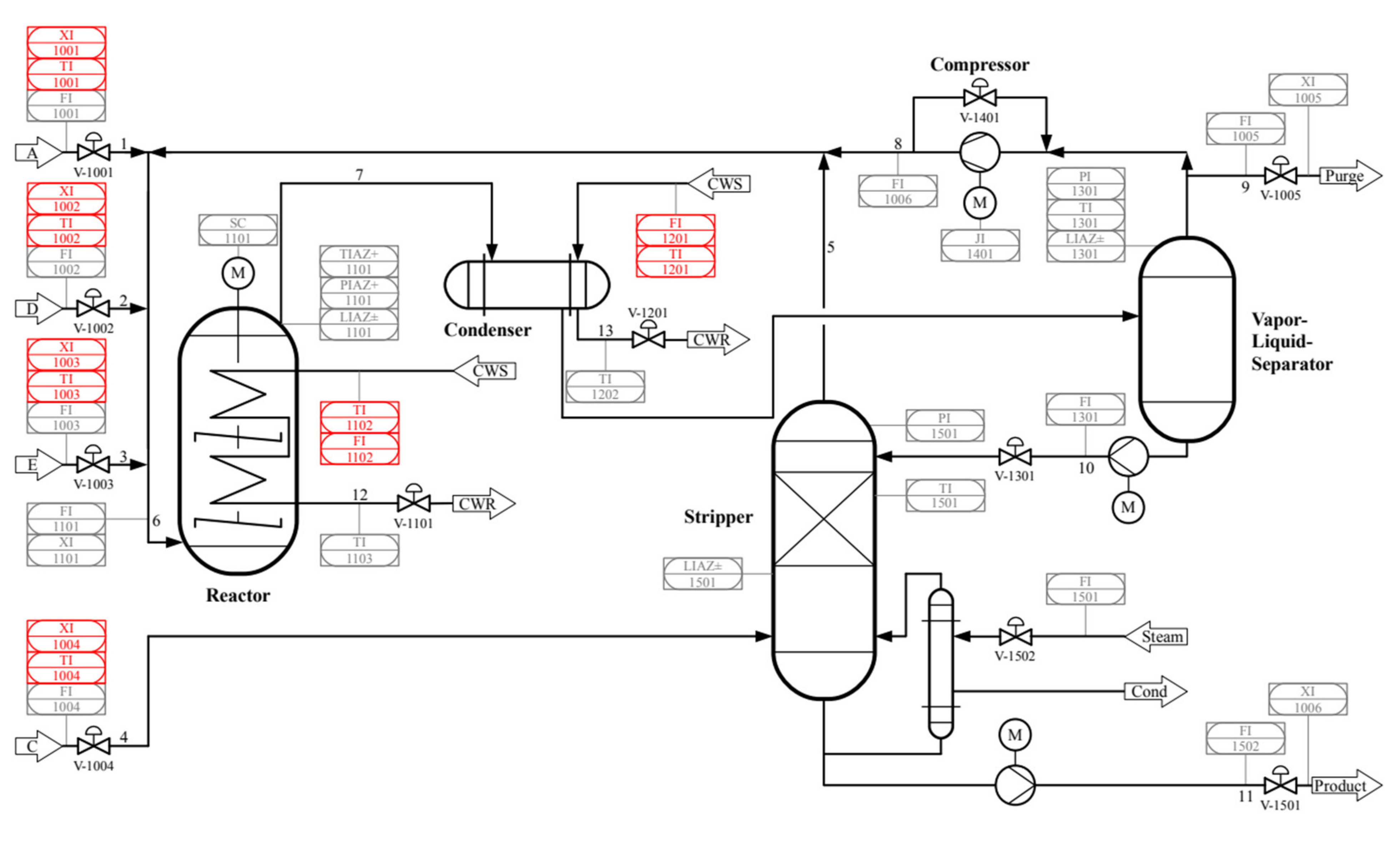
The TE process was widely cited as a benchmark for studies in control, optimization and fault diagnosis. The flowchart of the TE benchmark process is depicted in Figure 5 [44].

The TE process includes five units: a reactor, condenser, compressor, vapor or liquid separator and stripper. It simulates 21 types of faults. Details of the fault conditions are presented in

Table 1. Process faults for the Tennessee–Eastman process.

Fault Number	Description	Type
01	A/C feed ratio, B composition constant (Stream4)	Step
02	B composition, A/C ratio constant (Stream4)	Step
03	D feed (Stream2)	Step
04	Reactor cooling water inlet temperature	Step
05	Condenser cooling water inlet temperature	Step
06	A feed loss (Stream1)	Step
07	Header pressure loss—Reduced availability (Stream4)	Step
08	A, B and C composition (Stream4)	Random
09	D feed temperature (Stream2)	Random
10	C feed temperature (Stream4)	Random
11	Reactor cooling water inlet temperature	Random
12	Condenser cooling water inlet temperature	Random
13	Reaction kinetics	Slow drift
14	Reactor cooling water valve	Sticking
15	Condenser cooling water valve	Sticking
16–20 21	Unknown Valve position constant (Stream 4)	Unknown Constant position

.

The data came from the Matlab simulation code of the TE process built by the University of Washington. The sampling interval in the simulation was 3 min, and the number of data features was 52. There were two cases of data in the original report. Each case contained 22 sets of data, which included normal state data and 21 types of fault state data. We used the first case of data to begin a simulation in the normal state for 1 h, and the simulation was continued for 24 h after adding the disturbance. For the second case, the simulation was started in the normal state for 8 h and then continued for 40 h after the disturbance was added. The first case included 10,580 samples, and the second case included 21,120 samples, so the total sample size for model training and testing was 31,700. The ratio of the training set to the test set was 4:1. The data input format of the training and testing process of the model was the sample * feature.

3.2. Results and Discussion

The first step in improving the algorithm was to perform noise reduction on the historical data with lifting wavelets. Before choosing the threshold function, this paper used SNR to determine the optimal number of decomposition levels. The SNRs of different decomposition layers are shown in

Table 2. SNRs of different decomposition layers.

Number of Layers	0	1	2	3	4	5
SNR	113.5	125.12	130.15	136.9	125.4	122.2

.

According to the comparison of the SNRs of different decomposition layers, the best wavelet decomposition layer for the TE process would be three layers.

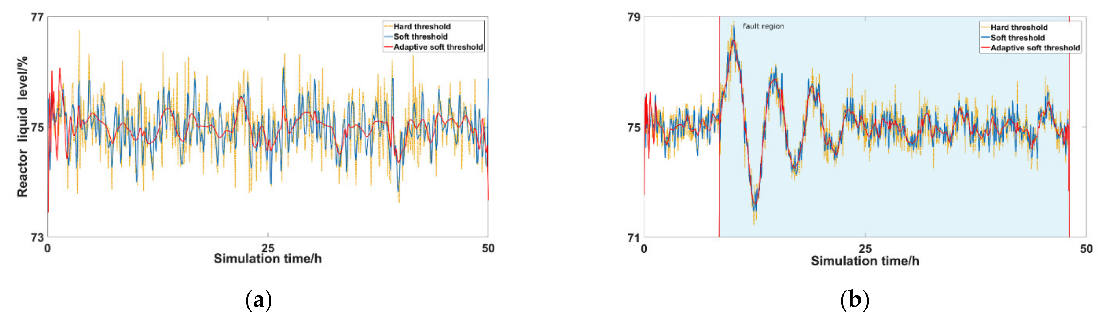
This study used three kinds of threshold methods to perform three sets of comparative experiments on the monitoring variables of the TE process. The monitoring variable in Figure 6a is the reactor liquid level, which corresponds to the data of the TE process that was continuously simulated for 50 h under normal conditions with a sampling interval of 3 min. The monitoring variable in Figure 6b is the reactor liquid level, which corresponds to the data after the TE process was simulated for 8 h under normal conditions and the fault 1 disturbance signal was added, and the simulation continued for 40 h. It can be observed from the figure that the data processed by the adaptive soft threshold method had fewer high-frequency disturbance signals than those processed by the soft and hard threshold methods, and the graph change trend was more stable.

According to the test results, the RMSE of the hard threshold method was 0.506, and the soft threshold method’s was 0.421. The RMSE of the adaptive soft threshold method under different adaptive coefficients is presented in

Table 3. The RMSE of adaptive soft threshold noise reduction under different values of $k$.

$$\mathit{k}$$	0	1	2	4	6	7	10
RMSE	0.0784	0.0421	0.0346	0.0328	0.0214	0.0362	0.0459

.

After testing, the noise reduction effect was best when $k=6$. In comparison with the traditional fixed threshold, the adaptive soft threshold method could remove the noise signal more effectively and retain the effective signal.

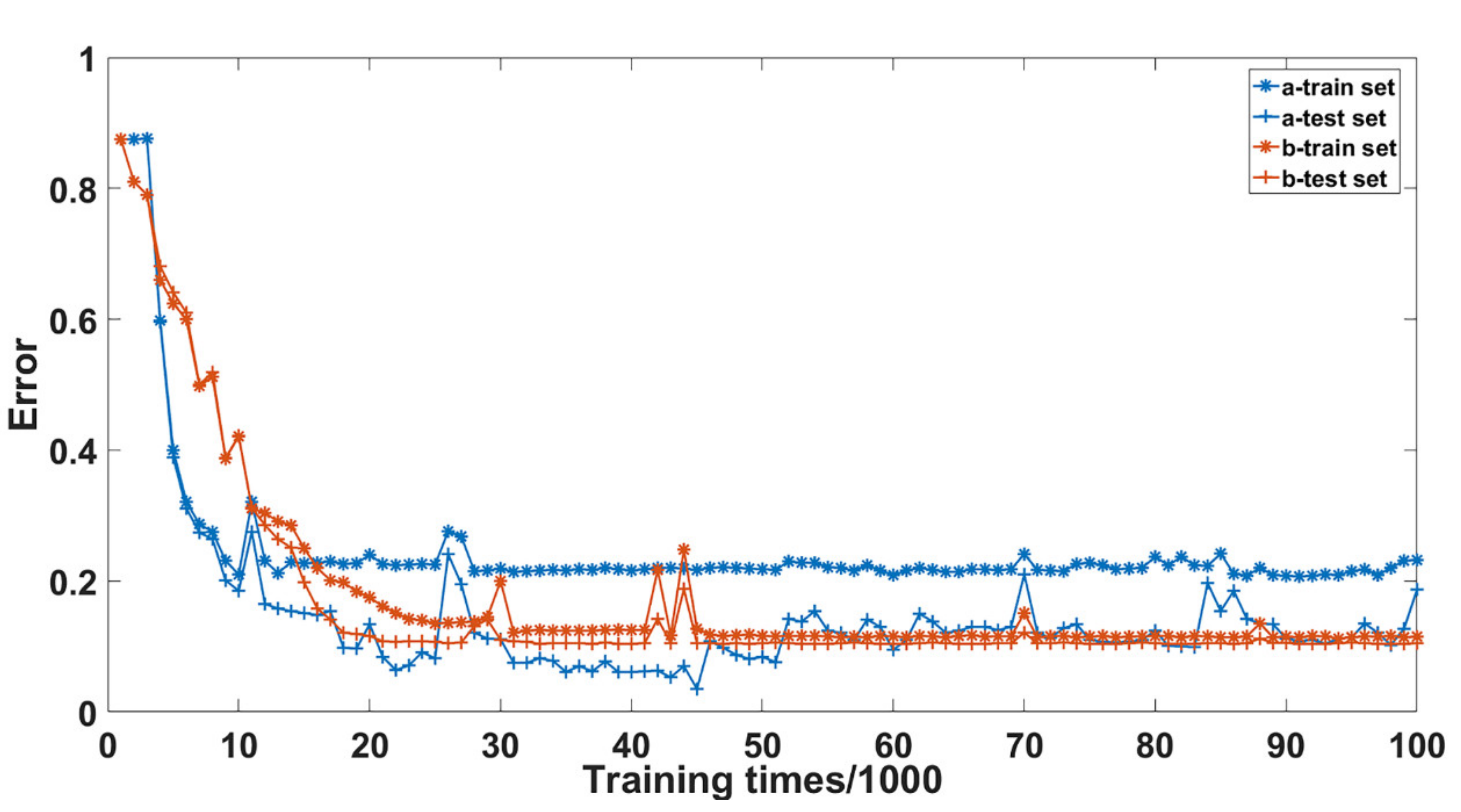
Then, the denoised data were normalized, and the training set was input into the first RBM for training. All RBM training was completed through an unsupervised greedy algorithm initialization layer by layer. After training all the RBMs, the back propagation algorithm was used as a means to fine-tune the structure and weight the parameters of the entire network with the label data corresponding to the training samples as the output target. Finally, the optimal combination of parameters was selected by minimizing the error. Figure 7 depicts the error curve during the adjustment process.

In Figure 7, the label a represents the sample size of each batch of updated data during the fine-tuning process without adding a penalty factor for 640 iterations. Label b represents the sample size of each batch of updated data after the penalty factor is added 640 times, and the horizontal axis also indicates that it is calculated every 1000 iterations. It can be observed from the figure that the training process without the penalty factor had oscillation or even divergence. Although the training process with the penalty factor was slower in convergence, it gradually converged to a lower range as the number of training times increased.

To obtain a suitable fault diagnosis model, we tested different hyperparameters, including the number of layers of the neural network, the number of neurons per layer, the learning rate, the number of pretraining and fine-tuning rounds, the momentum and the size of the batch, to improve its performance. Our final DBN model included six layers of neurons, with 50, 50, 30, 20 and 22 present on each layer. The batch sizes in the pretraining and fine-tuning stages were 80 and 634, respectively. The learning rate was 0.00005. In the fine-tuning phase, the training rate was 0.0005, and the training rate was reduced to 0.00001. After the training rate was reduced to 0.00001, the training was continued for 75,000 iterations. The number of pre-training sessions was divided into two stages. First, the momentum parameter was 0.5 for 100 pretraining iterations, and then it was 0.8 for 200 pretraining iterations. The number of updated data samples per batch in the pretraining phase was 160, and the number of updated data samples per batch in the fine-tuning phase was 640. The optimal penalty coefficient was iterated by the penalty parameter to be 0.00000005.

After unsupervised learning, the classification layer was added to the feature extraction model, and the label data were used for training. For each fault state and normal state, the following defines the fault diagnosis rate (FDR) and false positive rate (FPR) [28]:

$$FDR=\frac{p}{total count of this state samples}$$

(24)

$$FPR=1-\frac{q}{total count of other state samples}$$

(25)

where $p$ is the count of this state’s samples that are classified to this state and $q$ is the count of other state samples that are classified to another state.

The fault diagnosis results of the TE process need to be compared with other machine learning methods. This paper chose PCA, the Bayesian method and the SSVM method to compare the FDR and compare the FPR with the original DBN and the enhanced DBN. The results are shown in

Table 4. Comparison of the FDRs and FPRs of different fault diagnosis methods (Columns A, B, C, D, E, F and G refer to the PCA [45], Bayesian method [46], SSVM [21], original DBN, enhanced DBN, ALW-DBN and DCNN [26], respectively).

Fault Type	FDR (%)							FPR (%)
	(A)	(B)	(C)	(D)	(E)	(F)	(G)	(D)	(E)	(F)	(G)
Fault 01	100.0	100.0	95.0	99.0	100.0	100.0	98.6	0.0	0.0	0.0	0.3
Fault 02	99.38	99.0	100.0	98.0	98.0	99.9	98.5	0.0	0.0	0.0	0.0
Fault 03	10.25	6.0	0.0	2.0	75.0	89.5	91.7	18.0	12.0	9.0	0.8
Fault 04	100.0	100.0	57.0	20.0	81.0	100.0	97.6	0.0	2.0	0.0	0.0
Fault 05	34.75	100.0	64.0	33.0	100.0	100.0	91.5	19.0	7.0	2.0	0.6
Fault 06	100.0	100.0	93.0	99.0	100.0	100.0	97.5	1.0	1.0	0.0	0.0
Fault 07	100.0	100.0	100.0	61.0	99.0	99.8	99.9	0.0	1.0	0.0	0.0
Fault 08	97.83	99.0	100.0	97.0	97.0	99.1	92.2	60.0	9.0	2.0	0.1
Fault 09	9.88	3.0	0.0	1.0	84.0	93.5	58.4	21.0	19.0	15.0	2.0
Fault 10	71.0	84.0	53.0	53.0	88.0	93.3	96.4	5.0	6.0	2.0	0.0
Fault 11	83.0	82.0	21.0	40.0	82.0	97.9	98.4	19.0	9.0	5.0	0.1
Fault 12	99.0	100.0	0.0	98.0	99.0	99.8	95.6	73.0	10.0	2.0	0.1
Fault 13	95.75	95.0	91.0	94.0	94.0	98.9	95.7	0.0	2.0	0.0	0.0
Fault 14	100.0	100.0	0.0	87.0	100.0	100.0	98.7	14.0	18.0	7.0	0.0
Fault 15	17.25	17.0	0.0	16.9	80.0	90.6	28.0	16.0	8.0	4.0	2.8
Fault 16	65.75	89.0	88.0	43.0	81.0	98.5	44.2	11.0	6.0	1.0	3.8
Fault 17	96.88	96.0	68.0	80.0	92.0	97.6	94.5	23.0	13.0	5.0	0.0
Fault 18	91.13	90.0	82.0	89.0	91.2	96.2	93.9	0.0	8.0	0.0	0.1
Fault 19	47.38	52.0	16.0	3.0	79.0	95.8	98.6	39.0	18.0	6.0	0.0
Fault 20	71.50	88.0	100.0	49.0	87.0	97.7	93.3	20.0	13.0	1.0	0.0
Fault 21	56.50	61.0	90.0	38.0	85.0	96.0	-	15.0	5.0	2.0	-
Average	74.58	79.09	58.0	57.2	90.1	97.33	88.2	16.9	7.95	3.0	0.5

.

When compared with the traditional method in terms of the FDR, it can be seen that the FDR of the ALW-DBN model proposed in this paper was higher than the other methods in most fault situations, and the average FDR was the highest among all methods, especially for faults 3, 9 and 15, indicating that the ALW-DBN model was more sensitive to the more difficult faults.

In order to further quantify the fault diagnosis performance, the FDT was introduced and compared with the DCNN method proposed by Wu et al. [26]. This article set several operating conditions and selected 17 faults for comparison. The comparison results of the 17 faults are shown in

Table 5. Comparison of FDT of the same simulation conditions.

	DCNN		ALW-DBN
A *	3 min		3 min
B *	40 h	20 h	40 h	20 h
C *	20	10	20	10
1	20	36	10	17
2	39	50	35	41
3	35	26	25	24
4	15	34	20	22
5	33	12	30	8
6	18	25	10	12
7	35	15	34	17
8	94	89	57	48
10	82	57	49	34
11	45	45	47	39
12	52	33	30	21
13	100	82	77	55
14	24	24	15	21
17	124	123	88	69
18	45	56	20	10
19	64	53	72	41
20	146	163	54	59
Average	56	54	33.65	31.64

A *: sampling period; B *: fault simulating time; C *: sampling time length.

.

It can be seen that the ALW-DBN method proposed in this paper was better than the DCNN in FDT. The reason for this was that the ALW-DBN network not only eliminated the errors generated within the network training but also eliminated the noise outside the TE process and restored the true signal value, reducing the time required for training.

4. Case Study of an Acid Gas Absorption Process from Natural Gas

4.1. Acid Gas Adsorption Process Description

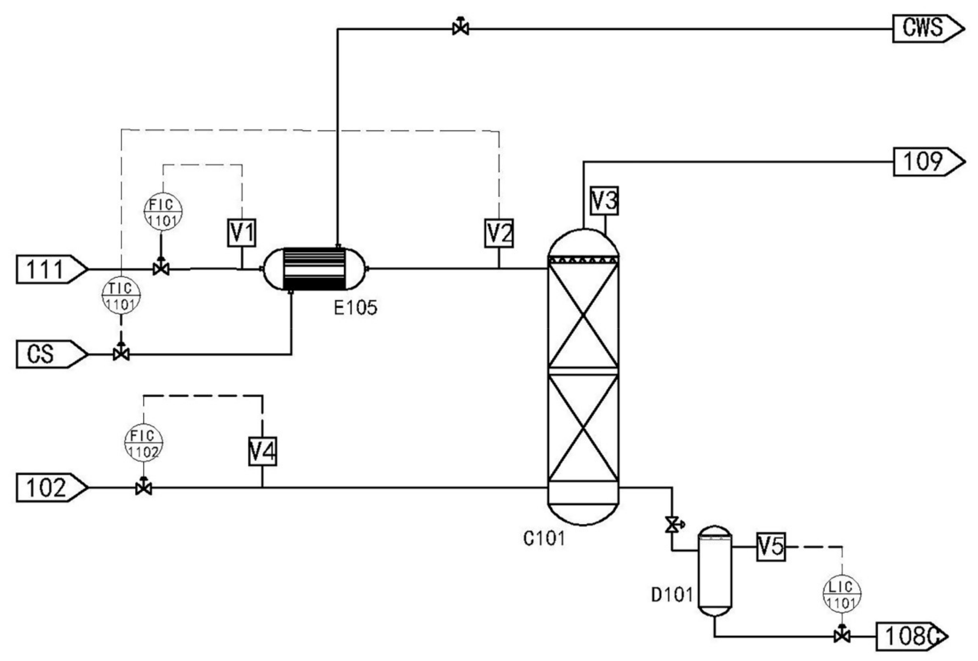
Methyldiethanolamine (MDEA) is often used as an absorbent in chemical processes to absorb acid gases. A flowchart of the typical absorption process is depicted in Figure 8.

Stream 111 is the absorbent MDEA. It first exchanges heat with cooling water at room temperature through the heat exchanger E-105 and then is cooled to 21 °C. Then, it enters the absorption tower C-101 from the top. The raw material gas stream 102 enters the absorption tower C-101 from the bottom, flows countercurrently with the absorbent MDEA and absorbs acid gases (H2S and CO2) from the natural gas. The overhead gas of the absorption tower C-101 is natural gas containing a large amount of moisture, which then enters the downstream dehydration system for further dehydration and purification to meet the national natural gas standards. The bottom product of the absorption tower C-101 is rich amine liquid containing acid gas. After heat exchange, the rich amine liquid enters the regeneration tower to resolve the acid gas and regenerate the absorbent. According to the piping and instrument diagram (P&ID) chart, the following variables are present: V1 is the absorbent MDEA volume flow rate; V2 is the absorption tower’s absorbent feed temperature; V3 is the absorption tower’s top pressure; V4 is the the natural gas feed flow; and V5 is the bottom liquid level height of absorption tower. The enhanced DBN and ALW-DBN models were tested and compared for this real chemical process.

4.2. Results and Discussion

To test the adaptability and accuracy of the enhanced DBN and ALW-DBN in situations with different amplitudes of noise, we used HYSYS to perform a dynamic simulation of the acid gas absorption process. The transfer function module of HYSYS was used to adjust the process variables (PVs) through the control variables. Noise was generated through transfer functions with standard deviations of 1, 2, 4, 6, 8 and 10 in different simulation runs. In this process, four types of faults were introduced to the normal situation: fault 1, where the inlet temperature of the heat exchanger slowly rose to 31 °C; fault 2, where the normal absorbent composition was MDEA (0.48), and water (0.49), which slowly changed to MDEA (0.08) and water (0.92), and the acid gas composition was reduced; fault 3, where the gas molar flow rate of 5202 kmoL/h was set to 7000 kmoL/h under normal conditions; and fault 4, where the bottom product outlet valve of the absorption tower was adjusted, namely with the valve opening being reduced by 10%. Finally, the PV values of all modules were generated and analyzed.

According to the actual simulated industrial data, the optimal wavelet decomposition layer was determined by the selection of different wavelet layers. The signal-to-noise ratios of different wavelet layers are shown in

Table 6. SNRs of different decomposition layers in the acid gas absorption process.

Noise Standard Deviation	1	2	4	6	8	10
Number of layers	2	2	3	4	5	6
SNR	45.12	47.55	52.21	57.89	65.2	70.15

.

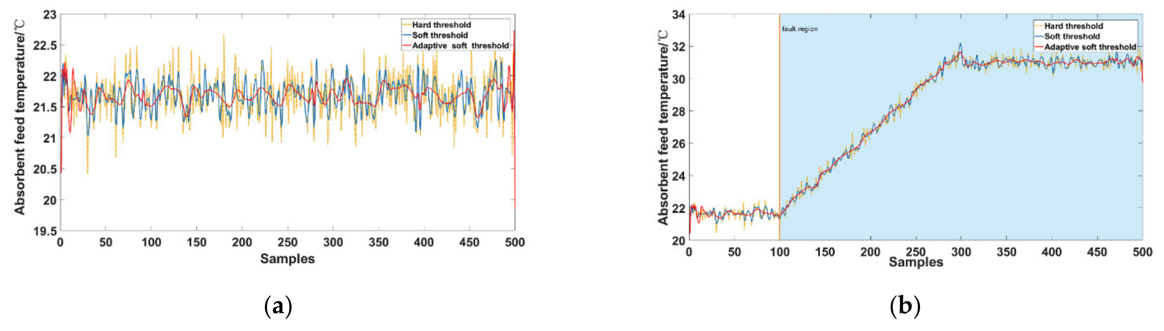
The noise standard deviation was also larger, and more layers needed to be decomposed. The corresponding SNR was also larger. Then, we selected 80% of the simulation results as the training set and the rest as the test set. The noise standard deviation was set to two. The noise reduction effect of variable 2—the absorption tower’s absorbent feed temperature—and the comparison between variable 2 before and after noise reduction in normal conditions and fault 1 are shown in Figure 9.

For the actual industrial process, the hard threshold noise reduction effect was not ideal, as shown in Figure 9. The adaptive soft threshold method could remove most of the noise existing in the data and display the most original state of the data, which had good performance in practical industrial applications. The selection of adaptive wavelet coefficients under different noise standard deviations is presented in

Table 7. Selection of adaptive wavelet coefficients under different noise standard deviations.

Noise Standard Deviation	2	4	6	8	10
$k$	4	5	6	7	9
RMSE	0.01245	0.01725	0.02146	0.02322	0.01795

.

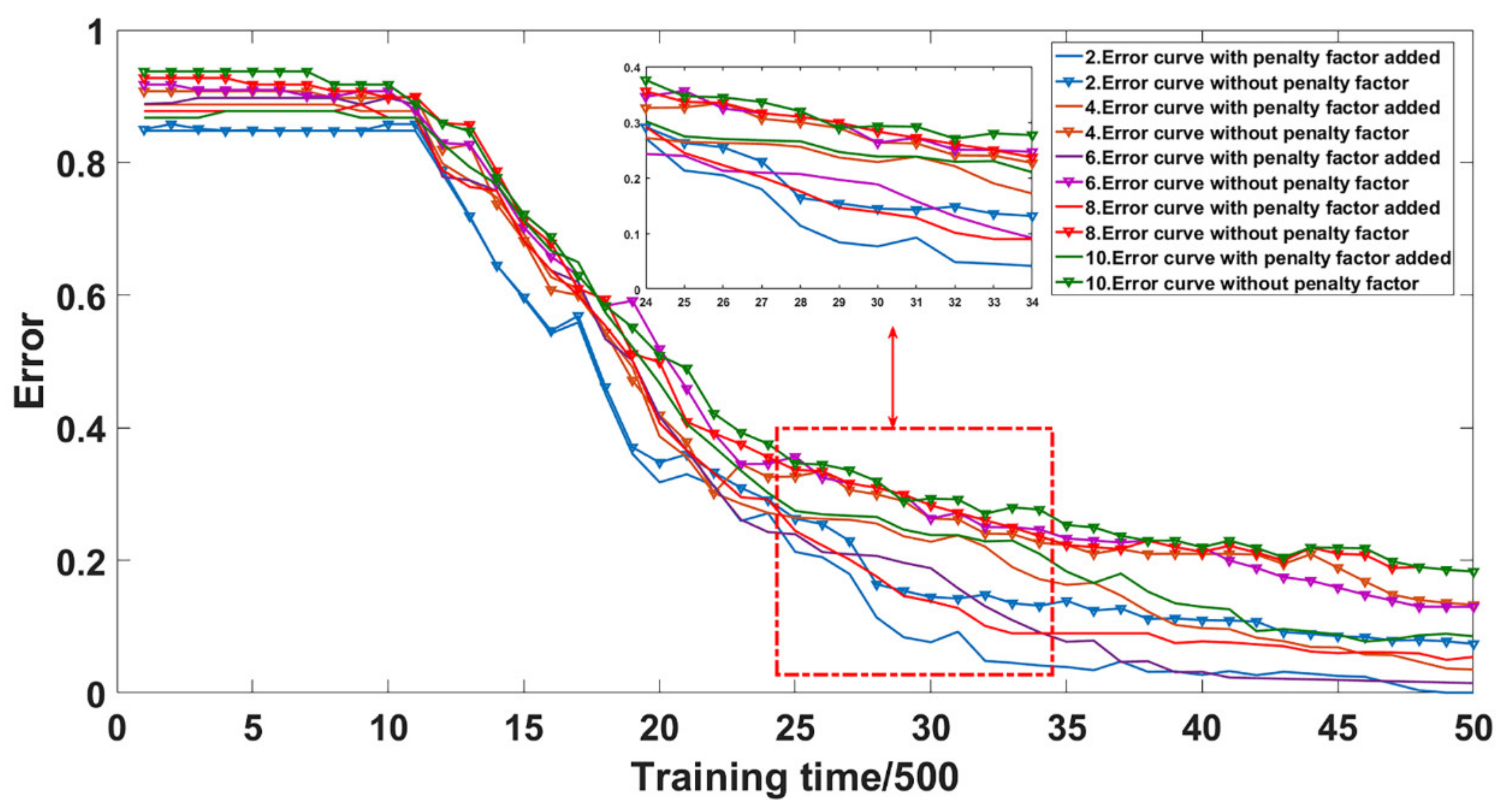
The adaptive wavelet coefficient k under different standard deviations could perform adaptive coefficient matching to different noises to achieve the greatest degree of noise reduction. Subsequent network training was prepared. Then, the denoised data were input into the ALW-DBN model for training. In the training process, the penalty factor was set to calculate the training error. Under different noise standard deviations, the influence of the penalty factor addition on the ALW-DBN model training error is shown in Figure 10.

The training results show that under the influence of noise with different standard deviations, the ALW-DBN model with a penalty factor was better than the model without a penalty factor. The iterative selection mechanism of penalty factors selected the optimal penalty factors for different systems and eliminated the cumulative error of each layer of the RBM during the training process. The overall DBN training mechanism was optimized.

The ALW-DBN model was applied to the fault diagnosis of the acid gas absorption process from natural gas under the influence of different levels of noise. The diagnosis results are listed in

Table 8. FDR (%) under different noise standard deviations.

FDR (%)	2		4		6		8		10		Average
	Enhanced DBN	ALW-DBN	Enhanced DBN	ALW-DBN	Enhanced DBN	ALW-DBN	Enhanced DBN	ALW-DBN	Enhanced DBN	ALW-DBN	Enhanced DBN	ALW-DBN
Fault 1	98	100	73	93	64	85	49	85	49	85	66.6	89.6
Fault 2	97	99	81	95	78	96	73	96	64	89	78.6	95
Fault 3	95	99	99	100	98	100	99	100	99	99	98.4	99.6
Fault 4	92	100	79	100	63	100	51	100	39	54	64.8	90.8
Average	96.25	99.5	82.75	97	75.75	95.25	68	95.25	62.75	81.75	77.1	93.75

and

Table 9. FPR (%) under different noise standard deviations.

FPR (%)	2		4		6		8		10		Average
	Enhanced DBN	ALW-DBN	Enhanced DBN	ALW-DBN	Enhanced DBN	ALW-DBN	Enhanced DBN	ALW-DBN	Enhanced DBN	ALW-DBN	Enhanced DBN	ALW-DBN
Fault 1	0.6	0.0	6.5	0.6	5.0	2.3	7.8	1.3	4.2	1.9	4.82	1.22
Fault 2	0.4	0.1	1.6	0.7	5.2	0.8	3.2	0.5	2.0	1.0	2.48	0.44
Fault 3	1.0	0.2	0.4	0.05	1.5	0.09	0.1	0.1	0.0	0.0	0.6	0.088
Fault 4	1.2	0.0	4.8	0.0	6.1	0.0	5.1	0.0	2.9	2.0	4.02	0.4
Average	0.55	0.075	3.33	0.3375	4.45	0.7975	3.8	0.475	2.28	1.23	2.98	0.537

.

In the case of different failure standard deviations, the larger the failure standard deviation, the less effective information could be extracted from the data. Therefore, the larger the failure standard deviation after the ALW method was used, the less effective fault information could be extracted by the deep belief network. Then, compared with the enhanced DBN for the FDT of the acid gas absorption process, the comparison results are shown in

Table 10. Comparing FDT with the enhanced DBN.

FDT (Min)	2		4		6		8		10		Average
	Enhanced DBN	ALW-DBN	Enhanced DBN	ALW-DBN	Enhanced DBN	ALW-DBN	Enhanced DBN	ALW-DBN	Enhanced DBN	ALW-DBN	Enhanced DBN	ALW-DBN
Fault1	8	4	8	5	9	5	10	6	10	6	9	5.2
Fault2	10	6	10	6	11	7	12	8	13	8	11.2	7
Fault3	9	5	10	6	10	6	11	8	12	8	10.4	6.6
Fault4	12	6	13	6	13	8	14	8	14	9	13.2	7.4
Average	9.75	5.25	10.25	5.75	10.75	6.5	11.75	7.5	12.25	7.75	10.95	6.55

.

Based on the comparison of the above diagnosis results, the performance of the ALW-DBN model was better than that of the enhanced DBN model without noise reduction. The results show that the DBN model optimized by the penalty factor was not accurate for different degrees of industrial noise diagnosis, and the diagnosis of the enhanced DBN model was more accurate than that of the single enhanced DBN model after eliminating redundant irrelevant noise by the adaptive soft threshold method. The diagnostic rates were 93.75% and 77.1%, respectively. However, for fault 3, when the gas molar flow rate was changed to 7000 kmoL/h, the diagnostic results of the enhanced DBN and ALW-DBN models were extremely similar because the gas flow rate of the 102A stream returned to 0 kmoL/h after the flow rate was stabilized, regardless of the added noise. When these two models were used to diagnose fault 3, the rates were almost identical. This suggests that fault 3 was insensitive to the choice between the enhanced DBN and ALW-DBN diagnostic models. Table 8 reveals that the ALW-DBN model was better in FPR than in the enhanced DBN model for each fault condition. The results show that the ALW-DBN model maintained high sensitivity to faults under the influence of different levels of noise. The average FPR was 0.537%. For the fault diagnosis time, the process data could extract effective features faster after adaptive noise reduction. Compared with the enhanced DBN model, the ALW-DBN model shortened the average FDT by 4.4 min. This shows the effectiveness of the ALW-DBN model in fault diagnosis.

5. Conclusions

To more accurately extract the fault characteristics and eliminate different noise levels, an ALW-DBN model based on ALW noise reduction and an enhanced deep confidence network were proposed. The adaptive soft threshold method could adaptively set the threshold function to match different data sets. The introduction of the penalty factor eliminated the cumulative error of each layer of RBM training in the DBN, thereby reducing the error of the final training result and improving the diagnosis accuracy. By using the data after adaptive wavelet denoising as the input data of the enhanced DBN, the two optimization algorithms were combined to form a complete ALW-DBN fault diagnosis model.

For the TE process, two types of noise reduction comparisons between the normal and fault data were performed. The results indicate that adaptive soft threshold noise reduction is more suitable for an enhanced DBN model. In comparison with the original DBN model, the enhanced DBN model and the ALW-DBN model for the diagnosis rates of 21 types of faults, the results indicate that the ALW-DBN model had the best diagnosis effect, with an average FDR of 96.21% and an FPR of 3.0%. Compared with other machine learning methods, it had a relatively large improvement in FDR and FPR. Then, compared with the DCNN in the FDT, the results show that the average FDT of the ALW-DBN model was 33.65 min, which was better than the DCNN result. This proves that the enhanced DBN model combined with adaptive wavelet noise reduction could yield better diagnostic results.

The ALW-DBN model exhibited excellent performance at different noise levels during the acid gas adsorption process. When the standard deviation of the noise was less than 8, the FDR of the ALW-DBN model was greater than 95%, and the average FDR of 5 different noises was 93.75%. In comparison with the enhanced DBN method, the diagnosis rate was 77.1%, and the average FPR of the ALW-DBN model was 0.537%, whereas that of the enhanced DBN model was 2.98%. It has been proven that the ALW-DBN model exhibits good diagnostic accuracy and noise adaptability for actual chemical processes with different noise effects. For FDT, the process data could extract effective features faster after adaptive noise reduction. Compared with the improved DBN model, the ALW-DBN model shortened the average FDT by 4.4 min. This shows the effectiveness of the ALW-DBN model in fault diagnosis.

Presently, the ALW-DBN model has some advantages in the application of industrial chemical process. However, due to the embedding of an iterative penalty optimization algorithm, the training of the ALW-DBN model becomes more time-consuming. At the same time, the model has errors in identifying fault types that do not exist in the training process, and its autonomous learning ability is too weak. Additionally, compared with the DCNN method, the DBN has obvious disadvantages in extracting the time information of chemical data. These shortcomings will limit the practical application of this method in complex chemical processes. In the future, we will discuss how to strengthen the universality of the method and how to improve the effect of the method, which will help formulate safe and reliable management measures and effective accident prevention plans for the maintenance of industrial chemical processes.

References

- Dai, Y.; Cheng, F.; Wu, H.; Wu, D.; Zhao, J. Chapter Five-Data driven methods. In Methods in Chemical Process Safety; Khan, F.I., Amyotte, P.R., Eds.; Elsevier: Amsterdam, The Netherlands, 2020; Volume 4, pp. 167–203. [Google Scholar]
- Alauddin, M.; Khan, F.; Imtiaz, S.; Ahmed, S. A Bibliometric Review and Analysis of Data-Driven Fault Detection and Diagnosis Methods for Process Systems. Ind. Eng. Chem. Res. 2018, 57, 10719–10735. [Google Scholar] [CrossRef]
- Wang, X.; Shen, C.; Xia, M.; Wang, D.; Zhu, J.; Zhu, Z. Multi-scale deep intra-class transfer learning for bearing fault diagnosis. Reliab. Eng. Syst. Saf. 2020, 202, 107050. [Google Scholar] [CrossRef]
- Saeed, U.; Jan, S.U.; Lee, Y.-D.; Koo, I. Fault diagnosis based on extremely randomized trees in wireless sensor networks. Eng. Syst. Saf. 2021, 205, 107284. [Google Scholar] [CrossRef]
- Jiang, W.; Wang, C.; Zou, J.; Zhang, S. Application of Deep Learning in Fault Diagnosis of Rotating Machinery. Processes 2021, 9, 919. [Google Scholar] [CrossRef]
- Park, Y.-J.; Fan, S.-K.S.; Hsu, C.-Y. A Review on Fault Detection and Process Diagnostics in Industrial Processes. Processes 2020, 8, 1123. [Google Scholar] [CrossRef]
- Xiao, S.; Lu, Z.; Xu, L. Multivariate sensitivity analysis based on the direction of eigen space through principal component analysis. Reliab. Eng. Syst. Saf. 2017, 165, 1–10. [Google Scholar] [CrossRef]
- Shirali, G.A.; Mohammadfam, I.; Ebrahimipour, V. A new method for quantitative assessment of resilience engineering by PCA and NT approach: A case study in a process industry. Reliab. Eng. Syst. Saf. 2013, 119, 88–94. [Google Scholar] [CrossRef]
- Aljunaid, M.; Tao, Y.; Shi, H. A Novel Mutual Information and Partial Least Squares Approach for Quality-Related and Quality-Unrelated Fault Detection. Processes 2021, 9, 166. [Google Scholar] [CrossRef]
- Cai, L.; Tian, X. A new fault detection method for non-Gaussian process based on robust independent component analysis. Process Saf. Environ. Prot. 2014, 92, 645–658. [Google Scholar] [CrossRef]
- Cai, L.; Tian, X.; Chen, H. Nonlinear process fault diagnosis using kernel ICA and improved FDA. IFAC Proc. Vol. 2013, 46, 736–741. [Google Scholar] [CrossRef]
- Pilario, K.E.; Shafiee, M.; Cao, Y.; Lao, L.; Yang, S.-H. A Review of Kernel Methods for Feature Extraction in Nonlinear Process Monitoring. Processes 2020, 8, 24. [Google Scholar] [CrossRef] [Green Version]
- Lavoie, F.B.; Muteki, K.; Gosselin, R. A novel robust NL-PLS regression methodology. Chemom. Intell. Lab. Syst. 2019, 184, 71–81. [Google Scholar] [CrossRef]
- Tu, S.; Menke, R.A.L.; Talbot, K.; Kiernan, M.C.; Turner, M.R. Cerebellar tract alterations in PLS and ALS. Amyotroph. Lateral Scler. Front. Degener. 2019, 20, 281–284. [Google Scholar] [CrossRef] [PubMed]
- Sun, S.; Cui, Z.; Zhang, X.; Tian, W. A Hybrid Inverse Problem Approach to Model-Based Fault Diagnosis of a Distillation Column. Processes 2020, 8, 55. [Google Scholar] [CrossRef] [Green Version]
- Hasani, G.; Daraei, H.; Shahrnoradi, B.; Gharibi, F.; Maleki, A.; Yetilmezsoy, K.; McKay, G. A novel ANN approach for modeling of alternating pulse current electrocoagulation-flotation (APC-ECF) process: Humic acid removal from aqueous media. Process Saf. Environ. Prot. 2018, 117, 111–124. [Google Scholar] [CrossRef]
- Li, F.; Wang, W.H.; Xu, J.; Yi, J.; Wang, Q.S. Comparative study on vulnerability assessment for urban buried gas pipeline network based on SVM and ANN methods. Process Saf. Environ. Prot. 2019, 122, 23–32. [Google Scholar] [CrossRef]
- Xu, S.; Hashimoto, S.; Jiang, Y.; Izaki, K.; Kihara, T.; Ikeda, R.; Jiang, W. A Reference-Model-Based Artificial Neural Network Approach for a Temperature Control System. Processes 2020, 8, 50. [Google Scholar] [CrossRef] [Green Version]
- Kulkarni, A.; Jayaraman, V.K.; Kulkarni, B.D. Knowledge incorporated support vector machines to detect faults in Tennessee Eastman Process. Comput. Chem. Eng. 2005, 29, 2128–2133. [Google Scholar] [CrossRef]
- Mahadevan, S.; Shah, S.L. Fault detection and diagnosis in process data using one-class support vector machines. J. Process Control 2009, 19, 1627–1639. [Google Scholar] [CrossRef]
- Yelamos, I.; Escudero, G.; Graells, M.; Puigjaner, L. Performance assessment of a novel fault diagnosis system based on support vector machines. Comput. Chem. Eng. 2009, 33, 244–255. [Google Scholar] [CrossRef]
- Jia, X.; Tian, W.; Li, C.; Yang, X.; Luo, Z.; Wang, H. A Dynamic Active Safe Semi-Supervised Learning Framework for Fault Identification in Labeled Expensive Chemical Processes. Processes 2020, 8, 105. [Google Scholar] [CrossRef] [Green Version]
- Xu, Y.; Shen, S.Q.; He, Y.L.; Zhu, Q.X. A Novel Hybrid Method Integrating ICA-PCA With Relevant Vector Machine for Multivariate Process Monitoring. IEEE Trans. Control Syst. Technol. 2019, 27, 1780–1787. [Google Scholar] [CrossRef]
- Lei, Y.; Jiang, W.; Jiang, A.; Zhu, Y.; Niu, H.; Zhang, S. Fault Diagnosis Method for Hydraulic Directional Valves Integrating PCA and XGBoost. Processes 2019, 7, 589. [Google Scholar] [CrossRef] [Green Version]
- Manogaran, G.; Varatharajan, R.; Priyan, M.K. Hybrid Recommendation System for Heart Disease Diagnosis based on Multiple Kernel Learning with Adaptive Neuro-Fuzzy Inference System. Multimed. Tools Appl. 2018, 77, 4379–4399. [Google Scholar] [CrossRef]
- Wu, H.; Zhao, J.S. Deep convolutional neural network model based chemical process fault diagnosis. Comput. Chem. Eng. 2018, 115, 185–197. [Google Scholar] [CrossRef]
- Liu, Y.; Yang, Y.; Feng, T.; Sun, Y.; Zhang, X. Research on Rotating Machinery Fault Diagnosis Method Based on Energy Spectrum Matrix and Adaptive Convolutional Neural Network. Processes 2021, 9, 69. [Google Scholar] [CrossRef]
- Zhang, Z.; Zhao, J. A deep belief network based fault diagnosis model for complex chemical processes. Comput. Chem. Eng. 2017, 107, 395–407. [Google Scholar] [CrossRef]
- Wang, Y.L.; Pan, Z.F.; Yuan, X.F.; Yang, C.H.; Gui, W.H. A novel deep learning based fault diagnosis approach for chemical process with extended deep belief network. ISA Trans. 2020, 96, 457–467. [Google Scholar] [CrossRef]
- Yu, J.; Yan, X. Layer-by-Layer Enhancement Strategy of Favorable Features of the Deep Belief Network for Industrial Process Monitoring. Ind. Eng. Chem. Res. 2018, 57, 15479–15490. [Google Scholar] [CrossRef]
- Lee, W.H.; Ozger, M.; Challita, U.; Sung, K.W. Noise Learning Based Denoising Autoencoder. IEEE Commun. Lett. 2021, 1. [Google Scholar] [CrossRef]
- Liu, R.; Li, Y.; Wang, H.; Liu, J. A noisy multi-objective optimization algorithm based on mean and Wiener filters. Knowl. Based Syst. 2021, 228, 107215. [Google Scholar] [CrossRef]
- Sun, T.; Neuvo, Y. Detail-preserving median based filters in image processing. Pattern Recognit. Lett. 1994, 15, 341–347. [Google Scholar] [CrossRef]
- Li, X.; Zhou, K.; Xue, F.; Chen, Z.; Ge, Z.; Chen, X.; Song, K. A Wavelet Transform-Assisted Convolutional Neural Network Multi-Model Framework for Monitoring Large-Scale Fluorochemical Engineering Processes. Processes 2020, 8, 1480. [Google Scholar] [CrossRef]
- Ho, J.; Hwang, W.-L. Wavelet Bayesian Network Image Denoising. Ieee Trans. Image Process 2013, 22, 1277–1290. [Google Scholar] [CrossRef] [PubMed]
- Wang, J.; Wu, J.; Wu, Z.; Jeong, J.; Jeon, G. Wiener filter-based wavelet domain denoising. Displays 2017, 46, 37–41. [Google Scholar] [CrossRef]
- Davoudabadi, M.-J.; Aminghafari, M. A fuzzy-wavelet denoising technique with applications to noise reduction in audio signals. J. Intell. Fuzzy Syst. 2017, 33, 2159–2169. [Google Scholar] [CrossRef]
- Sweldens, W. The Lifting Scheme: A New Philosophy in Biorthogonal Wavelet Constructions. In Wavelet Applications in Signal and Image Processing III; The International Society for Optical Engineering: Bellingham, WA, USA, 1995; Volume 2569. [Google Scholar] [CrossRef]
- Wang, X.; Wang, K.; Lian, S. A survey on face data augmentation for the training of deep neural networks. Neural Comput. Appl. 2020, 32, 15503–15531. [Google Scholar] [CrossRef] [Green Version]
- Hinton, G. A practical guide to training restricted boltzmann machines. Momentum 2010, 9, 926–947. [Google Scholar]
- Hinton, G.E. Training products of experts by minimizing contrastive divergence. Neural Comput. 2002, 14, 1771–1800. [Google Scholar] [CrossRef]
- Hinton, G.E.; Dayan, P.; Frey, B.J.; Neal, R.M. The “wake-sleep” algorithm for unsupervised neural networks. Science 1995, 268, 1158–1161. [Google Scholar] [CrossRef]
- Sweldens, W. The Lifting Scheme: A Custom-Design Construction of Biorthogonal Wavelets. Appl. Comput. Harmon. Anal. 1996, 3, 186–200. [Google Scholar] [CrossRef] [Green Version]
- Bathelt, A.; Ricker, N.L.; Jelali, M. Revision of the Tennessee Eastman Process Model. Ifac Pap. 2015, 48, 309–314. [Google Scholar] [CrossRef]
- Yin, S.; Ding, S.X.; Haghani, A.; Hao, H.; Zhang, P. A comparison study of basic data-driven fault diagnosis and process monitoring methods on the benchmark Tennessee Eastman process. J. Process. Control 2012, 22, 1567–1581. [Google Scholar] [CrossRef]
- Jiang, Q.; Huang, B. Distributed monitoring for large-scale processes based on multivariate statistical analysis and Bayesian method. J. Process. Control 2016, 46, 75–83. [Google Scholar] [CrossRef]
Figure 1.
The illustration of the DBN network structure.
Figure 2.
Structure of the enhanced DBN.
Figure 3.
Wavelet lifting process.
Figure 4.
Framework of the ALW-DBN-based fault diagnosis method.
Figure 5.
TE benchmark process.
Figure 6.
Comparison of adaptive soft, soft and hard thresholds ((a) normal state; (b) fault 1 state).
Figure 7.
Error curve in the fine-tuning process when the updated sample size is 640 (a: no penalty factor added, b: penalty factor added).
Figure 8.
Acid gas adsorption process flow chart.
Figure 9.
Comparison of variable 2 before and after noise reduction between normal conditions and fault 1 ((a) normal condition; (b) fault 1 condition).
Figure 10.
Training error curve of the ALW-DBN model under different noise standard deviations.