Response Surface Methodology Routed Optimization of Performance of Hydroxy Gas Enriched Diesel Fuel in Compression Ignition Engines

Abstract

In this study, the response surface methodology (RSM) optimization technique was employed for investigating the impact of hydroxy gas (HHO) enriched diesel on performance, acoustics, smoke and exhaust gas emissions of the compression ignition (CI) engine. The engine was operated within the HHO flow rate range of 0–10 L/min and engine loads of 15%, 30%, 45%, 60% and 75%. The results disclosed that HHO concentration and engine load had a substantial influence on the response variables. Analysis of variance (ANOVA) results of developed quadratic models indicated the appropriate fit for all models. Moreover, the optimization of the user-defined historical design of an experiment identified an optimum HHO flow rate of 8 L/min and 41% engine load, with composite desirability of 0.733. The responses corresponding to optimal study factors were 25.44%, 0.315 kg/kWh, 117.73 ppm, 140.87 ppm, 99.37 dB, and 1.97% for brake thermal efficiency (BTE), brake specific fuel consumption (BSFC), CO, HC, noise, and smoke, respectively. The absolute percentage errors (APEs) of RSM were predicted and experimental results were below 5%, which vouched for the reliable use of RSM for the prediction and optimization of acoustics and smoke and exhaust emission characteristics along with the performance of a CI engine.

1. Introduction

The oil reserves are depleting rapidly and are only sufficient to meet the drastically increasing power demand for the next fifty years [1]. Energy demand is soaring at an unprecedented pace and the available sources are too meagre to satisfy the needs [2,3]. In this scenario, the consumption of diesel as a transportation fuel has also increased by about 40% over the last decade [4]. The agriculture sector makes a major contribution to diesel consumption [5,6] as heavy machinery uses diesel as a fuel [7]. Moreover, automotive diesel engines share 26% of total greenhouse gas emissions into the environment, which is an unignorable threat to the stability of the Earth [8,9,10]. This has motivated researchers to investigate alternative fuels, such as hydroxy gas (HHO) for the versatile dual-fuel compression ignition engines [11,12], to find clean, economical, and sustainable energy resources [13,14,15].

The emission and combustion characteristics of internal combustion engines are mainly governed by the chemical and physical properties of the burning fuel [16,17]. Hydroxy gas (HHO), also termed brown gas, has only hydrogen and oxygen in its structure, and provides clean-burning to control CO₂ emissions and produces pure water when employed in CI engines [17]. Although hydrogen has a favorable high-octane rating, specific energy content, and autoignition temperature, it alone is not an appropriate option as a primary fuel due to the high safety risks of pressurized storage tanks in vehicles [18,19,20,21]. Consequently, an onboard HHO generating unit can mitigate the operational and safety problems concerning hydrogen generation, transportation and storage [22,23]. However, it can only be used as an additive because the same amount of energy as released from combustion (240 kJ/mol) is mandatory for HHO production [24].

The use of HHO as an alternative fuel has been the focus of researchers for quite a long time. In this regard, Pushpendra Kumar Sharma et al. explored the influence of varying flow rates of HHO with varying engine loads and observed a maximum increase of 6.5% for BTE along with a reduction of 58%, 60%, and 49% in CO and HC emissions, and smoke for 0.75 L/min and a 10 kg load, respectively [25]. Conversely, Subramanian et al. reported a 7% decrease in BTE at 36 L/min of flow rate owing to the higher auto-ignition temperature of hydrogen, a non-homogeneous air–diesel–HHO mixture and incomplete combustion at higher flow rates [26]. Usman et al. conducted a comparative assessment of gasoline, LPG, and LPG–HHO blends and reported improved performance and emissions for HHO blended LPG as compared to neat LPG [27]. Similarly, in another study, CNG–HHO blend showed 15.4% higher brake power and reduced CO and HC emissions [28]. In addition, Hydroxy gas can also be used as a secondary additive with the blends of other liquid and gaseous fuels [22], such as bio-fuels, to improve the performance (BP and BSFC) and emissions (CO₂ and HC) of IC engines [26,29,30].

Over the last two decades, several studies have investigated the use of RSM optimization to improve engine operation along with pollutant reduction of diesel-fueled engines [31,32,33]. Samet Uslu defined RSM models of the emission and performance of an engine operated with a palm oil diesel blend. He found that the correlation coefficients of all models were 0.90. Moreover, the optimum palm oil percentage of 17.88% was identified by multi-response optimization [31]. Milind Yadav et al. used RSM for the prediction and optimization of the performance characteristics of an oxy–hydrogen blended gasoline fueled SI engine [34]. Moreover, the use of RSM for the prediction of the emission and performance of the biodiesel–diesel blend was conducted by Mustafa Aydın et al. They reported a 32% biodiesel ratio, engine load of 816 W, and 470 bar injection pressure for the best performance and minimal emissions [35].

The cited literature reveals that the use of RSM for the optimization of diesel engines has been extensively carried out. However, one of the important aspects of emissions, that is, acoustic emissions, has not been given attention. This study addresses this very issue. Further, CI engines have not been optimized by employing the RSM technique for performance, acoustic, smoke, and exhaust emissions of the diesel–HHO blend. In this study, HHO was introduced with diesel at a flow rate of 0–10 L/min at varying loads. Later, RSM was used for studying the individual interactions between the study factors along with the statistical significance of developed models. The optimization identified the use of HHO with diesel as an effective alternative fuel that promises improved performance and reduced emissions.

Section 2 describes the detailed experimental approach of this study utilizing hydroxy gas. The results are discussed in detail utilizing ANOVA analysis in Section 3. The work is optimized utilizing RSM and validated in Section 4 and Section 5, respectively. The study is concluded with recommendations and future research directions in Section 6.

2. Materials and Methods

This study used a 30 kW Perkins (AD 3.152), 91.4 mm bore length, four stroke diesel engine for experimentation. The specifications of the test engine are shown in

Table 1. Test engine specifications.

Factors	Narrative
Type/Make	AD 3.152/Perkins
Volumetric efficiency (percent)	85
Stroke (cm)	1.27
Bore (cm)	0.91
Number of nozzles	3
Diesel injection	17° before TDC

. The experiments were performed for different flow rates of HHO, ranging from 0 L/min to 10 L/min while loads were varied from 0–75%, with an equal increment of 15% for each strategic test run. The physicochemical properties of diesel and hydrogen are presented in

Table 2. Properties of test fuels.

Properties	Diesel	Hydrogen [28]
Physical state	Liquid	Gas
Specific gravity	0.83–0.86 @ 16 °C	0.000083
Stoichiometric A/F	14.5	34.2
Viscosity (at 40 °C) (mm2/s)	2.42	N/A
Boiling Range	160 to 366 °C	N/A
Cetane Number	57.86	-
Flash Point (°C)	59	N/A
Calorific Value (kJ/kg)	44,000	120,000

. Diesel fuel was directly supplied to the engine through the fuel injectors. However, HHO gas was supplied to the test engine intake manifold at varying flow rates for the diesel HHO mixture. The schematic of the experimental setup, which includes HHO generator, noise measuring meter, smoke meter, emission analyzer and electric heaters, is displayed in Figure 1. Brake thermal efficiency and brake specific fuel consumption were calculated numerically by utilizing calorific value (CV), brake power (BP), and fuel consumption (FC). The brake power was measured from the integrated control panel with heaters, which indicates the value of voltage and current at different load conditions, varied through electrical switches to turn on/off the heaters. In the experimental setup, heaters acted as a resistance load. The test engine was equipped with three phase AC generator having five breakers. Each breaker was equivalent to a load of 15%, which was applied to the engine through the generator. Simply, all the breakers turned on means the engine is operating on a load of 75%. Fuel consumption was determined by measuring time for the consumption of 100 mL of liquid fuel indicated by a gauged cylinder fixed adjacent to diesel containing tank while calorific value was obtained from Pakistan State Oil (PSO). HHO flow rate was ascertained from the rotameter connected at the output of the HHO generator. An emission analyzer (TESTO 350) was employed as a CO and HC emission content recorder, with a measuring sensitivity of 1 ppm CO, and 10 ppm HC. A smoke (opacity) meter (Wager 6500 manufactured by GasTech), which was in full compliance with the requirements of the SAE J1667 test criteria, was used to notice the smoke within a range of 0.0–100.0%. The engine noise level was measured with a sound level meter (UNI-T UT353), which can accurately measure 30–130 dB sound at a frequency response of 31.5 Hz to 8KHz.

HHO was generated by electrolysis of water, which is the most commonly used method. Alkaline hydroxides, for example, KOH and NaOH and so forth, were used for speeding up the reaction [36]. The HHO generation system included AC supply, load controller, transformer, rectifier, reactor, and bubbler. The maximum production capacity of the unit was 10 L/min. Potassium hydroxide (KOH) was used as a catalyst owing to its higher solubility and affinity for water [22,37]. The flow rate of the produced gas was controlled using a potentiometer which was directly dependent on the current passing through the cell.

3. Results and Discussion

3.1. Response Surface Methodology

RSM is a statistical technique used for the estimation of relationships between input and response variables. It adopts linear, quadratic, or higher-order polynomial functions to investigate the statistical significance of the study factors and their interactions. Moreover, the regression concept is used for the prediction and optimization of responses. Over the years, the use of RSM in engineering fields has shown welcome results in the prediction of complex systems.

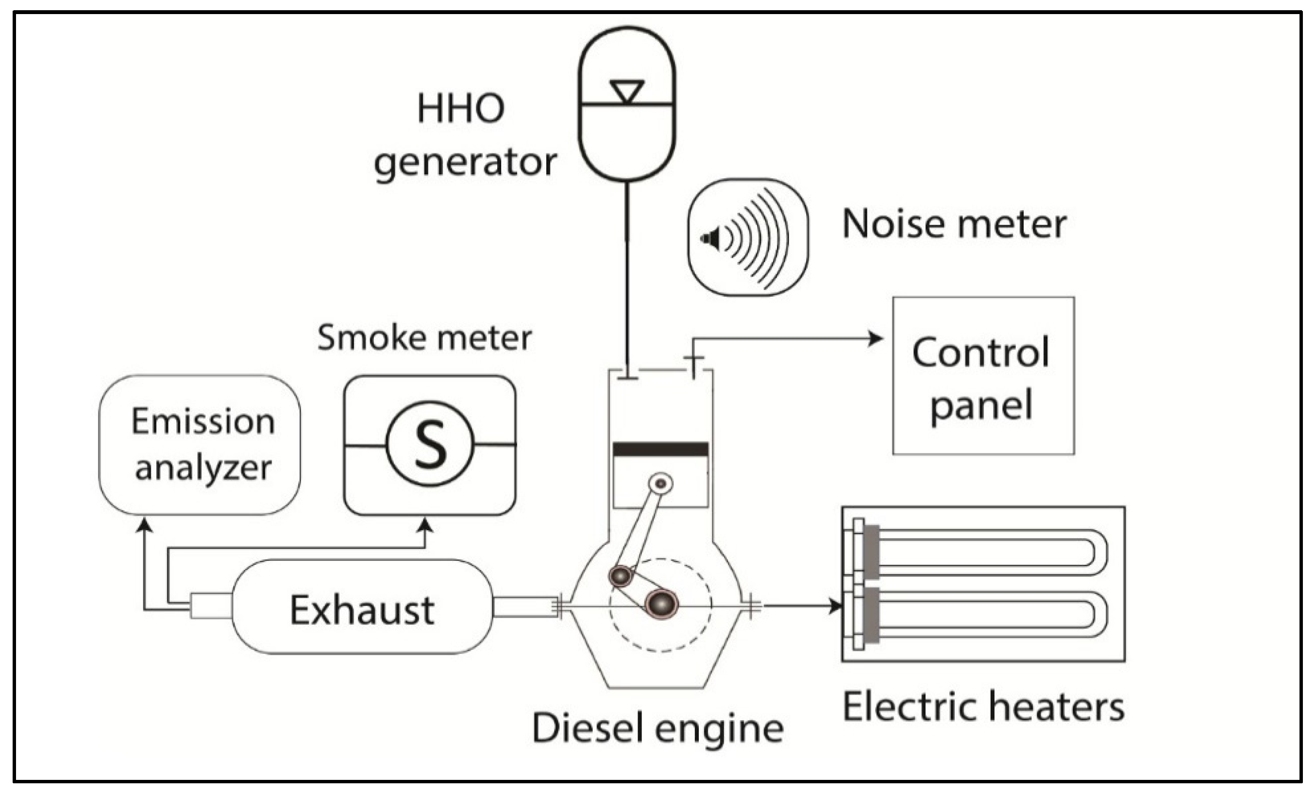
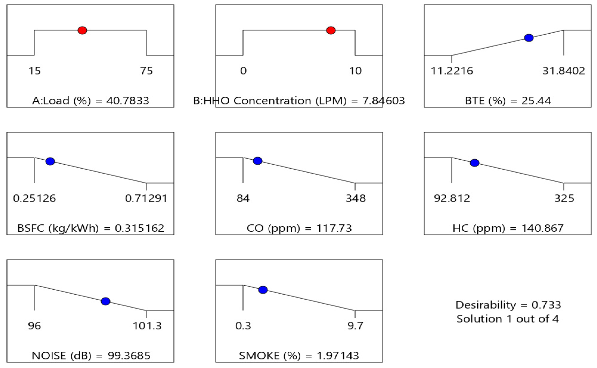
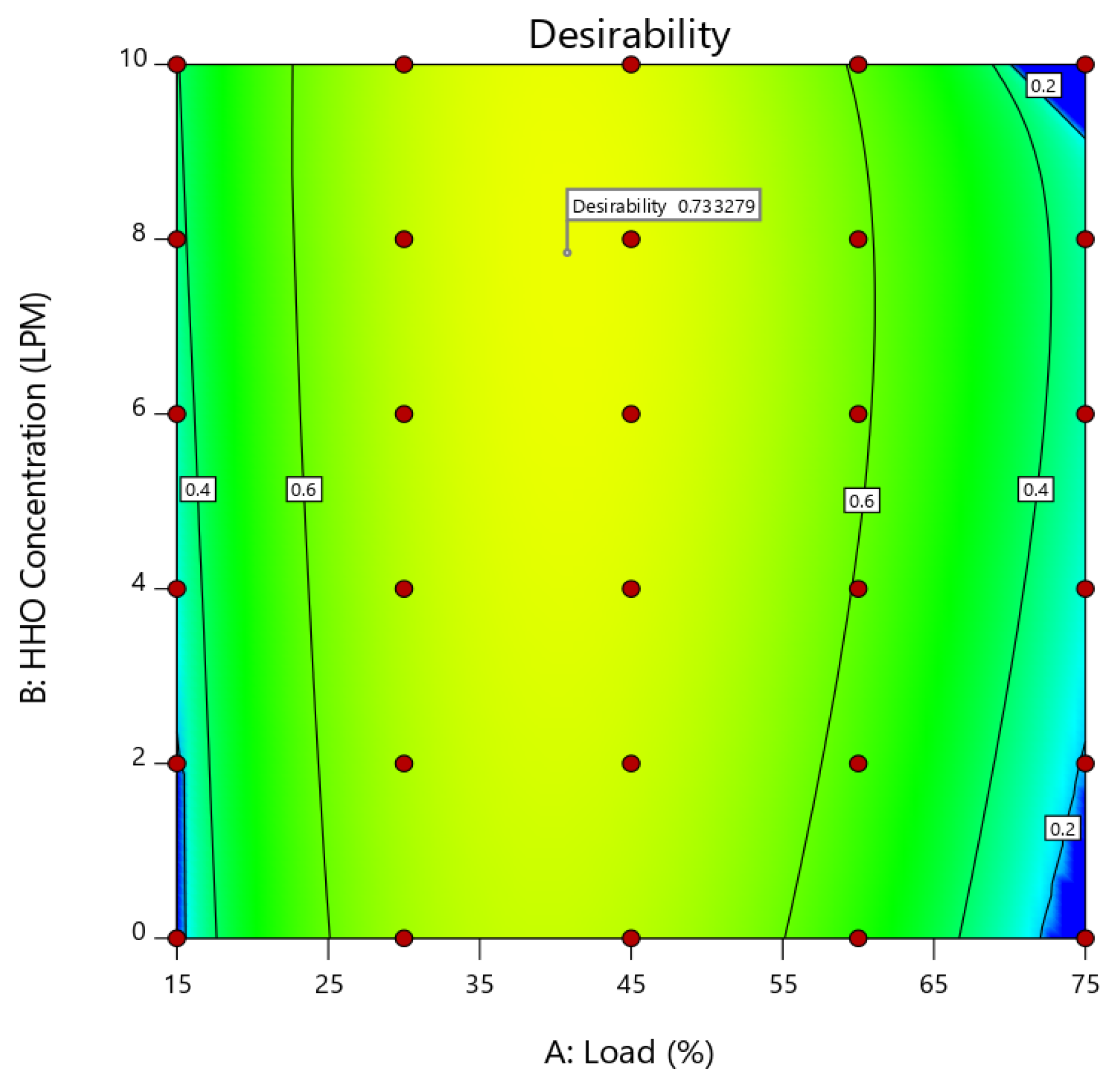
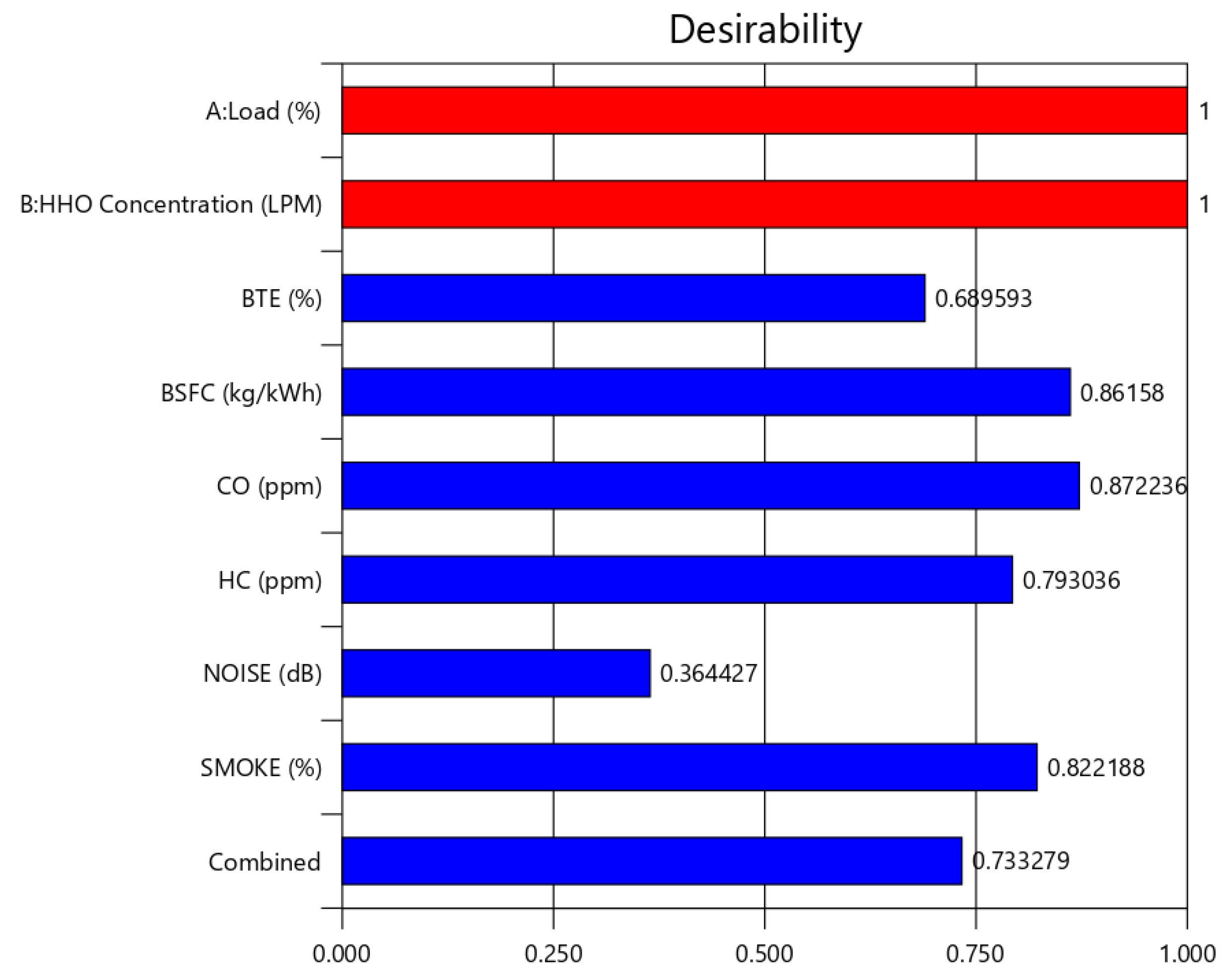
In the current study, the examined parameters were engine load and HHO concentration. Design-Expert version 11 was used for defining the multi-level historical design. The candidate set was created using user-defined discrete levels. Engine load and HHO concentration were assigned to four and six levels, respectively. The response variables measured were BTE, BSFC, CO, HC, noise, and smoke. The best fit model for each response was selected and analysis of variance (ANOVA) was applied for a better understanding of model attributes. In ANOVA, F is a probability distribution in different samplings, Df is degrees of freedom and the p-value is a statistical measure of variations in samples of a particular property. The decision rule for significance was benchmarked as a p-value less than 0.05. The percentage contribution (PC%) of each model term was calculated, which is a ratio of an aggregate of squared deviations to an individual sum of squares (SOS). PC% is a tool that provides a rough idea about the relative importance of study factors and the interactions.

3.2. ANOVA Results

The ANOVA results and fit statistics for BTE are presented in

Table 3. ANOVA results for BTE.

Source	Sum of Squares	Df	Mean Square	F-Value	p-Value	PC%
Model	1344.94	5	268.99	1980.51	<0.0001	99.7582
A-Load	1138.40	1	1138.40	8381.87	<0.0001	84.43851
B-HHO Concentration	47.75	1	47.75	351.56	<0.0001	3.541759
AB	7.30	1	7.30	53.76	<0.0001	0.541463
A²	151.34	1	151.34	1114.29	<0.0001	11.22534
B²	0.1454	1	0.1454	1.07	0.3111	0.010785
Residual	3.26	24	0.1358			0.241804
Cor Total	1348.20	29

. The F-value of 1980.51 and p-value less than 0.0001 show that the model for BTE is significant. Moreover, the R² value of 0.9976 (refer to

Table 4. Coefficient of determination for BTE.

Coefficient of Determination	Value
R2	0.9976
Adjusted R2	0.9971
Predicted R2	0.9958

) is close to positive unity and there is sufficient agreement between predicted and adjusted R². The p values from the ANOVA table show that both load and concentration of HHO are significant. However, the load is significantly contributing to aggregated variations with a PC% of 84.4 compared to fuel concentration (3.5%). The best fitted quadratic model from the fit summary was selected owing to the poor fit and aliased nature of linear and cubic models, respectively. The actual regression equation for BTE is given by Equation (1).

BTE (%) = 0.456285 + 0.793251 × Load − 0.00680684 ×Concentration + 0.00680858 × Load × Concentration − 0.0059656 ×Load² + 0.00697741 × Concentration².

(1)

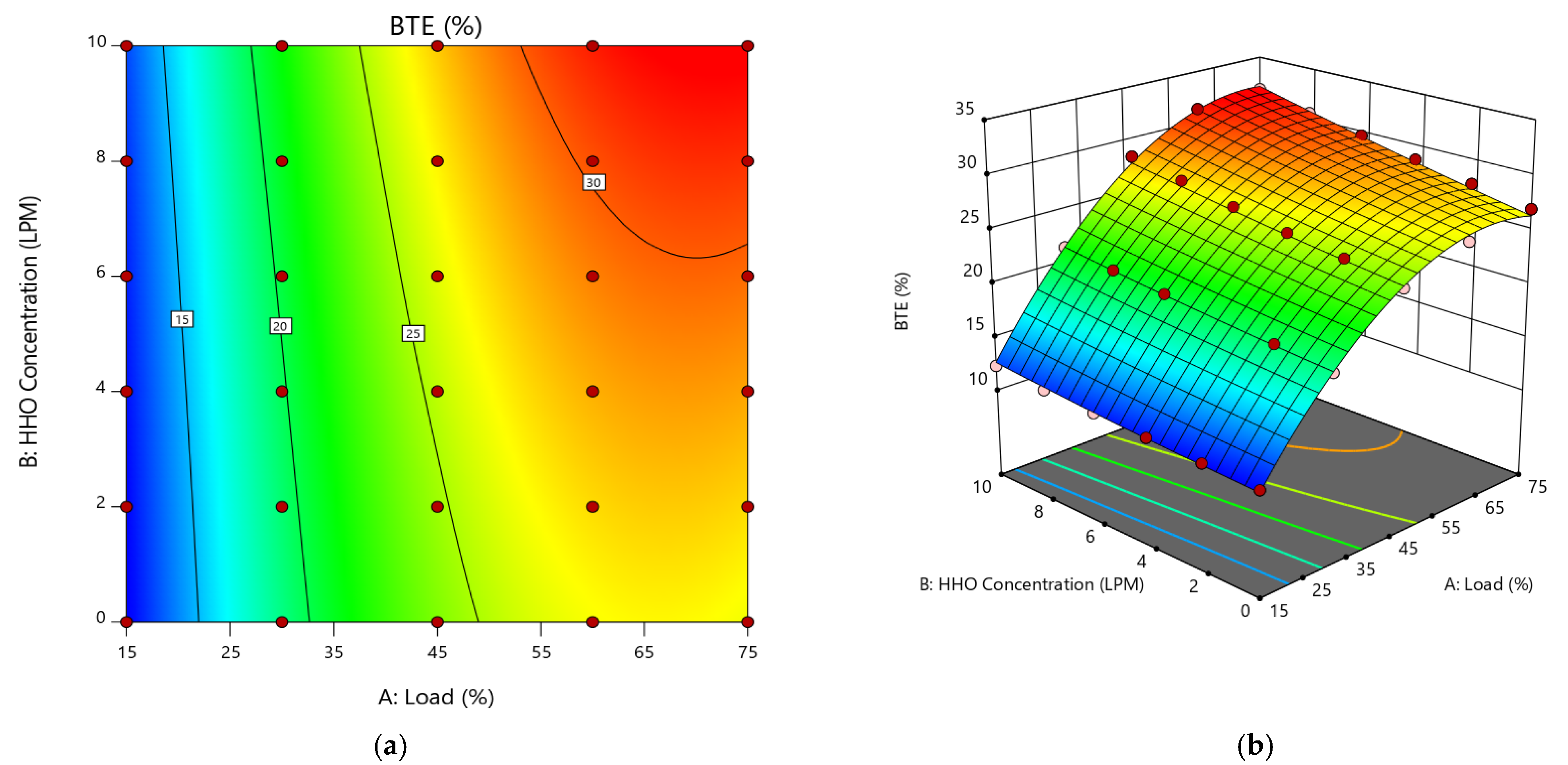
The contour plot (see Figure 2a) reveals the impact of load and fuel addition on BTE variation. The red color of the contour region advocates high engine BTE at high load and high HHO concentration. The color gradually shifted to red with an increase in HHO amount. The more explicit variation of response (BTE) is noticeable in Figure 2b. The 3D surface plot shows the rising curve of BTE with positive moments along the load and fuel axes. The maximum thermal efficiency is observable at an engine load of 75% and a 10 L/min flow rate of HHO. The improvement in BTE with HHO enrichment is due to the complete combustion of diesel in the presence of hydroxy gas which resulted from higher mean effective pressure near TDC, owing to the faster flame travel in the case of hydrogen. The dark and light circles above and below the surface represent the experimental and predicted values, respectively. Furthermore, the accuracy of the given models could be assessed using certain diagnostics tests and graphs. In general, small deviations between experimental and predicted results are desirable for efficient models. 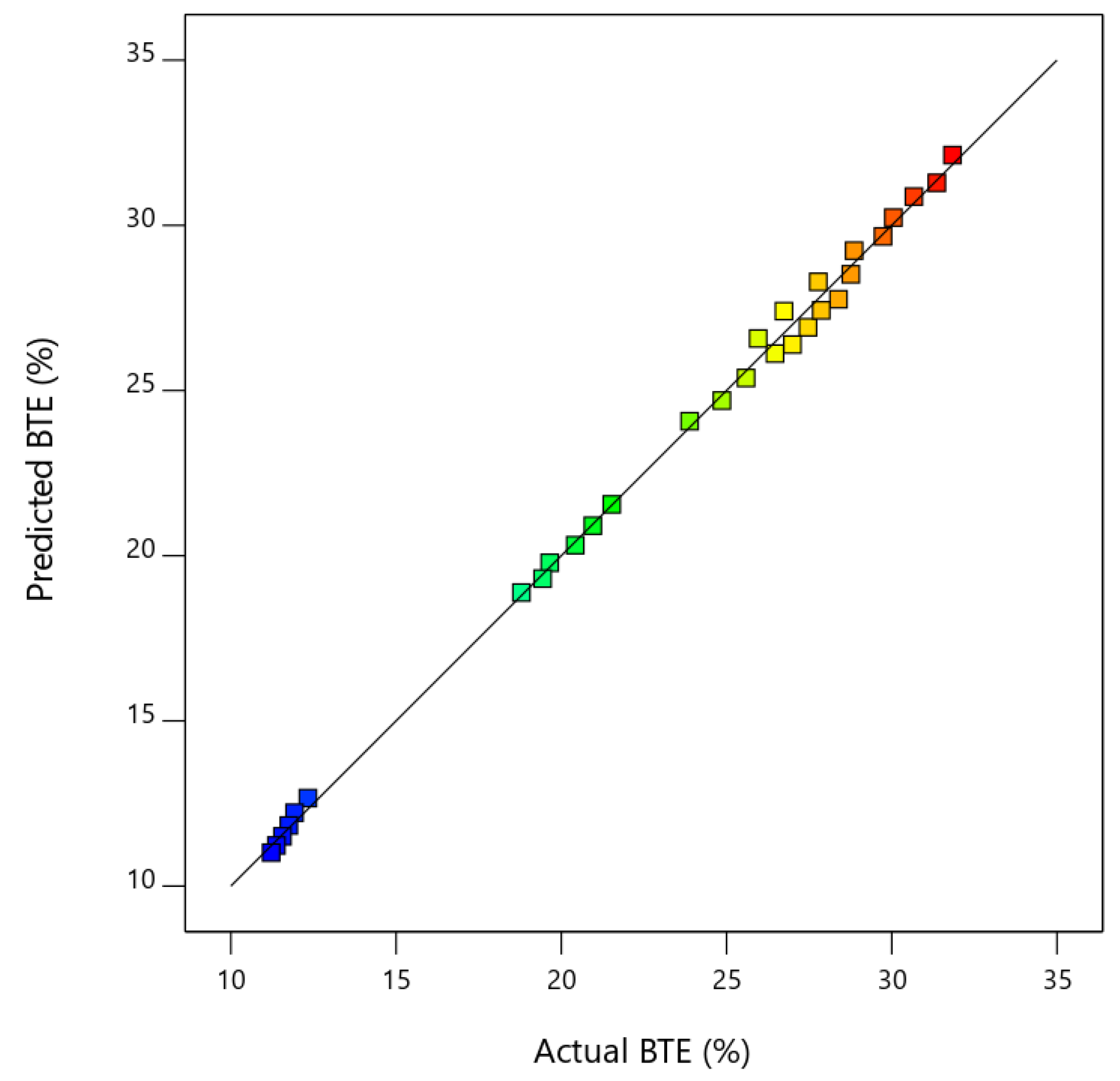Figure 3 shows a comparison of actual and predicted BTE. The minimal deviations of predicted values from actual data sets are testimony to a good fit of the quadratic regression model.

ANOVA results for the second response variable, BSFC, are shown in

Table 5. ANOVA results for BSFC.

Source	Sum of Squares	Df	Mean Square	F-Value	p-Value	PC (%)
Model	0.7029	5	0.1406	169.80	<0.0001	97.24682
A-Load	0.5275	1	0.5275	637.11	<0.0001	72.98008
B-HHO Concentration	0.0099	1	0.0099	11.95	0.0020	1.369673
AB	0.0001	1	0.0001	0.0927	0.7634	0.013835
A²	0.1655	1	0.1655	199.85	<0.0001	22.89707
B²	7.101 × 10−6	1	7.101 × 10−6	0.0086	0.9270	0.000982
Residual	0.0199	24	0.0008			2.753182
Cor Total	0.7228	29

. The model is significant owing to an F value of 169.80, a p-value less than the designated range, and R² (0.9725) close to 1, as indicated in

Table 6. Coefficient of determination for BSFC.

Coefficient of Determination	Value
R2	0.9725
Adjusted R2	0.9668
Predicted R2	0.9587

. The ANOVA findings show the significant effect of both load and HHO on fuel consumption. However, compared on a comparative scale, the load variations were found to have a greater impact on an engine than HHO concentration, as evidenced by PCs of 72.9% and 1.4%, respectively. The quadratic regression equation for BSFC on an actual scale is shown by Equation (2).

BSFC (kg/KWh) = 1.01215 − 0.0241143 × Load − 0.00582281 × HHO Concentration + 2.20781 × 10⁻⁵ × Load ×HHO Concentration + 0.000197256 × Load² − 4.87589 × 10⁻⁵ × HHO Concentration².

(2)

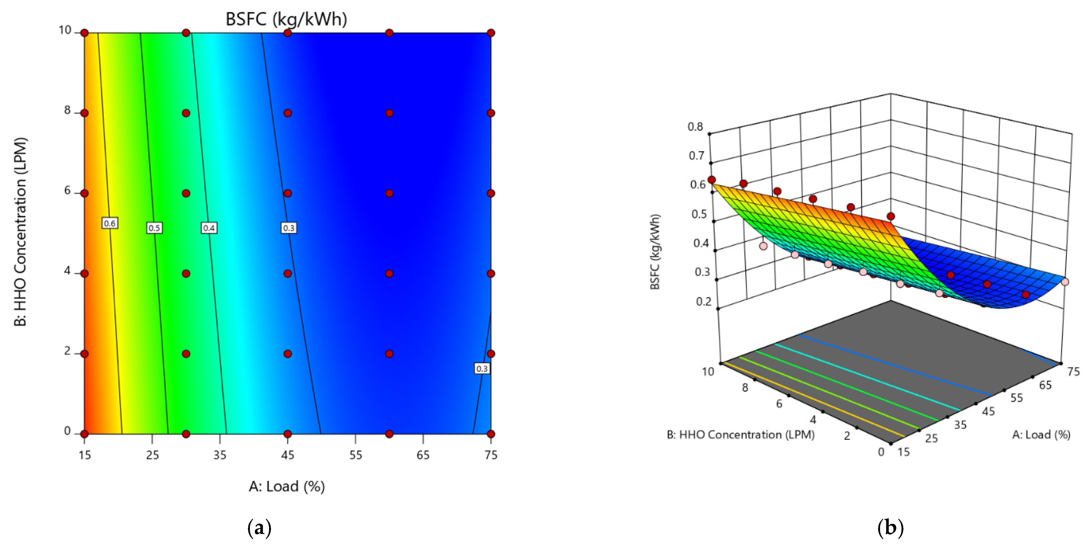
The effect of HHO addition and load on the fuel consumption trend of an engine is shown in Figure 4a,b. The contour plot in Figure 4a shows that fuel economy improved with successive addition of HHO to diesel at high loads. Moreover, it is also evident that, for the load range of 15–45%, there are more abrupt variations in BSFC compared to high loads, as indicated by a multi-color region. The response surface curve in Figure 4b shows the decreasing increasing trend of BSFC with load and fuel concentration. The sudden lift in the curve at the culmination is due to increased fuel demand at a high load owing to ample friction resistance. The improved fuel economy with HHO enrichment is primarily because of the higher calorific value of HHO and efficient combustion due to the lean diesel–HHO–air mixture [38,39]. 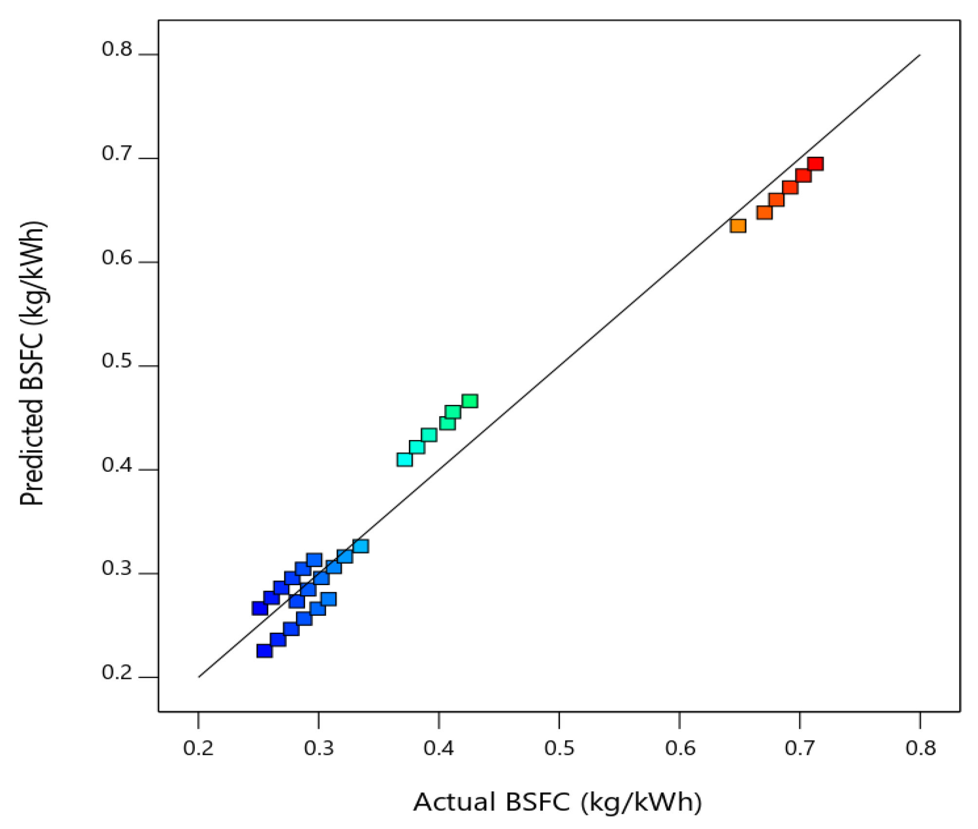The comparison of predicted and actual BSFC, as given in Figure 5, shows a bit of disorder data near the regression line. The disorderliness is due to the manual use of equipment in calculating BSFC. However, the deviations are not so large and therefore the model is acceptable.

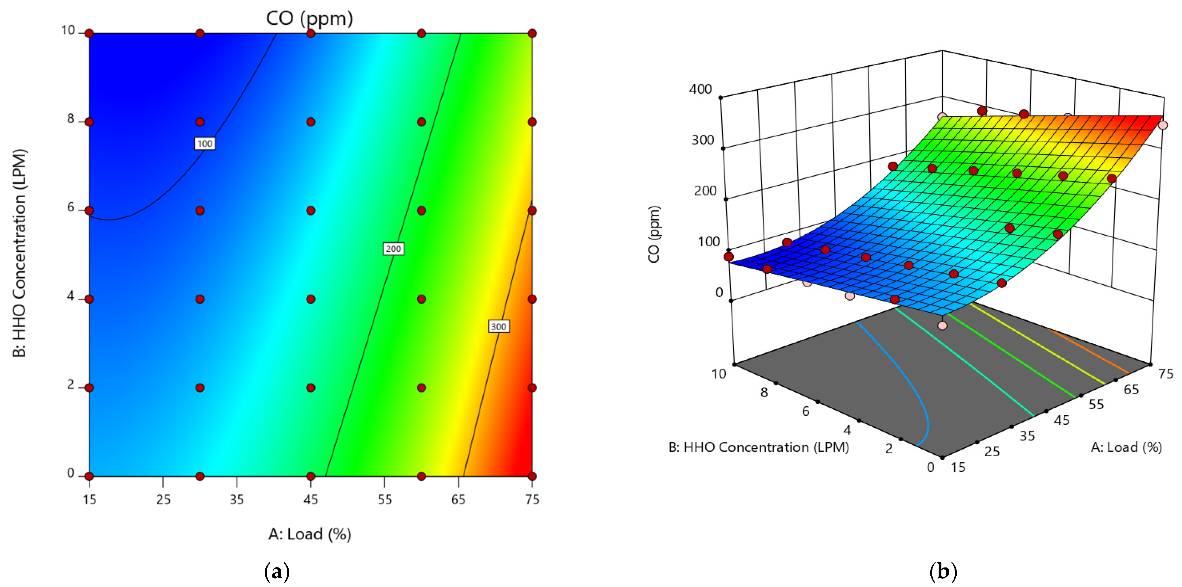
Similar to performance, quadratic models for emissions were also analyzed using ANOVA. The defined model for CO emissions was significant as shown in

Table 7. ANOVA results for CO.

Source	Sum of Squares	Df	Mean Square	F-Value	p-Value	PC%
Model	2.033 × 105	5	40,654.18	260.45	<0.0001	98.20
A-Load	1.635 × 105	1	1.635 × 105	1047.57	<0.0001	78.98
B-HHO Concentration	21,980.99	1	21980.99	140.82	<0.0001	10.62
AB	1307.48	1	1307.48	8.38	0.0080	0.63
A²	16,460.64	1	16,460.64	105.45	<0.0001	7.95
B²	2.14	1	2.14	0.0137	0.9077	0.00
Residual	3746.27	24	156.09			98.20
Cor Total	2.070 × 105	29

. The results revealed that both factors were significant; however, the percentage contribution of load to overall variations was greater compared to fuel concentration. Moreover, the R² value was 0.9819 (refer to

Table 8. Coefficient of determination for CO.

Coefficient of Determination	Value
R2	0.9819
Adjusted R2	0.9781
Predicted R2	0.9684

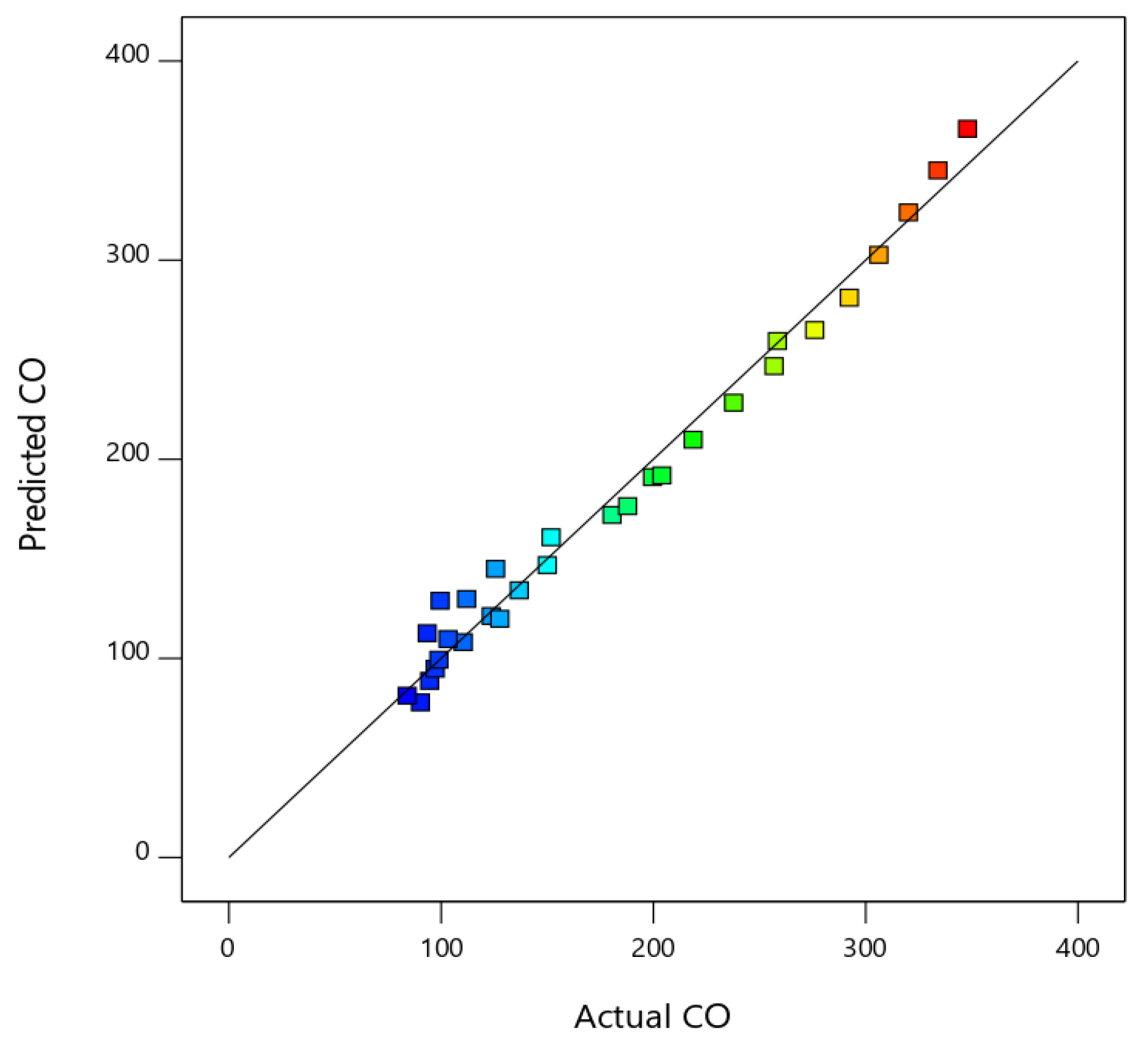
) and there was a reasonable agreement between adjusted and predicted R². In an attempt to see the accuracy of the selected model, the actual versus predicted description in Figure 6 could be used as a model accuracy measuring tool. It is discernible from the figure that the data points are near to the linear regression line and deviations are negligible. The CO emission regression equation on a coded scale is given by Equation (3).

CO (ppm) = 140.804 − 1.66356 × Load − 3.55691 × HHO Concentration − 0.0911124 × Load × HHO Concentration + 0.0622159 × Load² − 0.0267857 × HHO Concentration².

(3)

The variations in emissions of carbon monoxide with load and HHO concentrations are shown in Figure 7a,b. The contour plot (Figure 7a) provides a general illustration of the CO emission pattern of the engine subjected to various loads. The emissions are shown with the multi-color scheme, where blue stands for the minimum and red for the maximum. The response surface in Figure 7b depicts the CO variations with load and HHO. The main root of carbon monoxide generation is the partial burning of fuel inside the engine. The addition of hydroxy gas not only reduces the carbon content but also facilitates complete combustion which consequently reduces the emissions [40]. Therefore, a curve is seen to be following a decreasing trend in the presence of HHO.

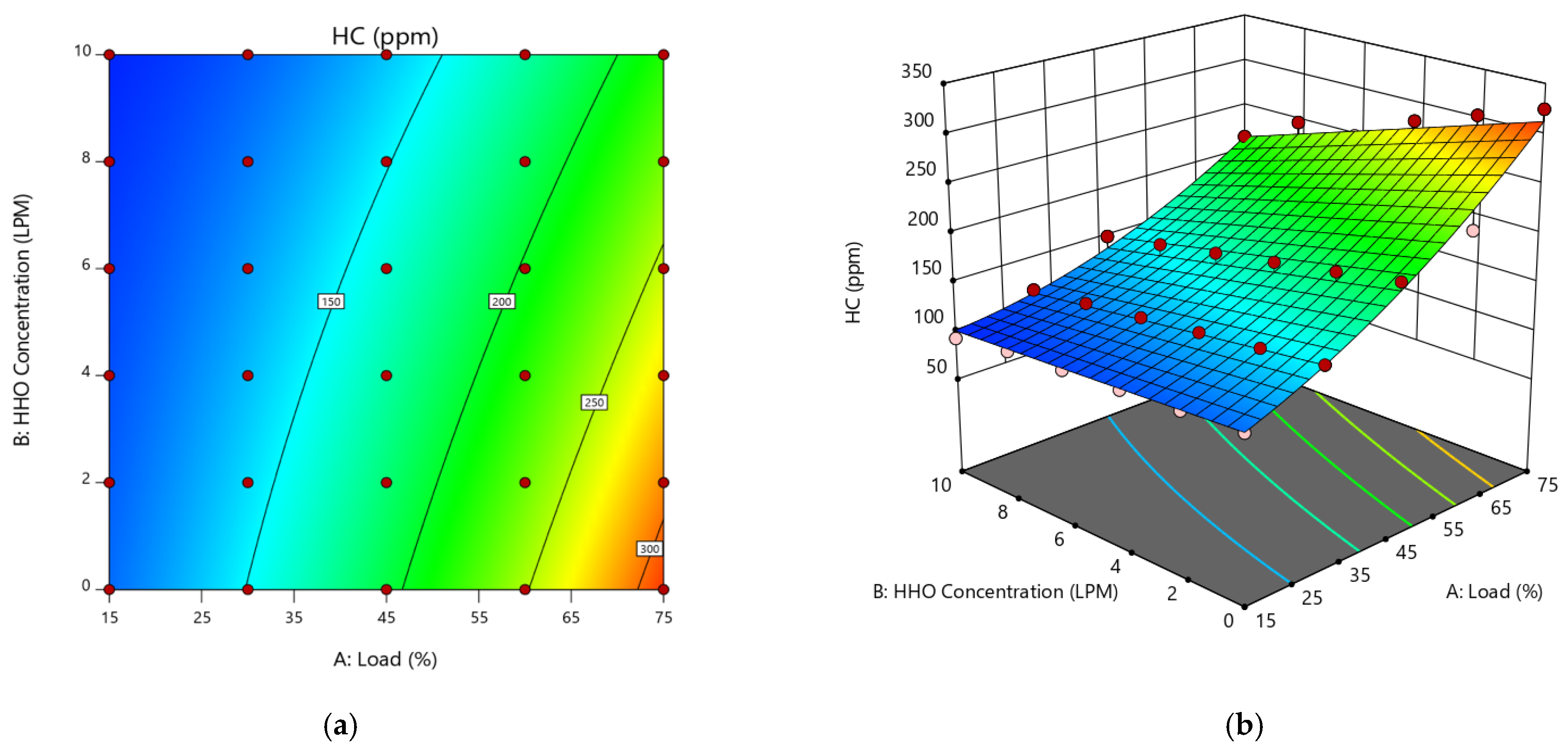
Similarly,

Table 9. ANOVA results for HC.

Source	Sum of Squares	Df	Mean Square	F-Value	p-Value	PC (%)
Model	1.065 × 105	5	21,306.90	176.60	<0.0001	97.32231317
A-Load	90,147.78	1	90,147.78	747.17	<0.0001	82.3792533
B-HHO Concentration	11,262.46	1	11,262.46	93.35	<0.0001	10.29191229
AB	2834.94	1	2834.94	23.50	<0.0001	2.590637732
A²	2289.29	1	2289.29	18.97	0.0002	2.092009374
B²	0.0595	1	0.0595	0.0005	0.9825	5.43726 × 10−5
Residual	2895.67	24	120.65			2.646134296

presents the ANOVA results of HC emission. The model selected and input variables are significant because of p values less than 0.005. The coefficient of determination, the R² value, however, is shown in

Table 10. Coefficient of determination for HC.

Coefficient of Determination	Value
R2	0.9735
Adjusted R2	0.9680
Predicted R2	0.9592

. Engine load and HHO concentration had percentage contributions of 82.4% and 10.3% respectively. The comparison of actual and predicted HC emissions in Figure 8 shows that the selected model is accurate. Equation (4) gives the predicting regression equation of HC emissions.

HC (ppm) = 94.8363 + 1.16673 × Load + 0.320067 × HHO Concentration − 0.134163 × Load × HHO Concentration + 0.0232022 × Load² + 0.00446429 × HHO Concentration².

(4)

The detailed effect of varying factors on hydrocarbon emissions is shown in Figure 9a,b. The addition of HHO reduced HC emissions for all concentrations and the minimum emissions were found to be for 10 L/min, as shown in Figure 9a. Similarly, the response surface shows the emission variations of each fuel combination and is seen following a decreasing trend. The presence of hydroxy gas reduces HC, while carbon present in lubricating oil and primary diesel fuel is oxidized by excessive oxygen and high combustion temperatures inside the cylinder. Moreover, a relatively short quenching distance and a wider flammability range in the case of gaseous fuel have improved the engine performance in this regard [41].

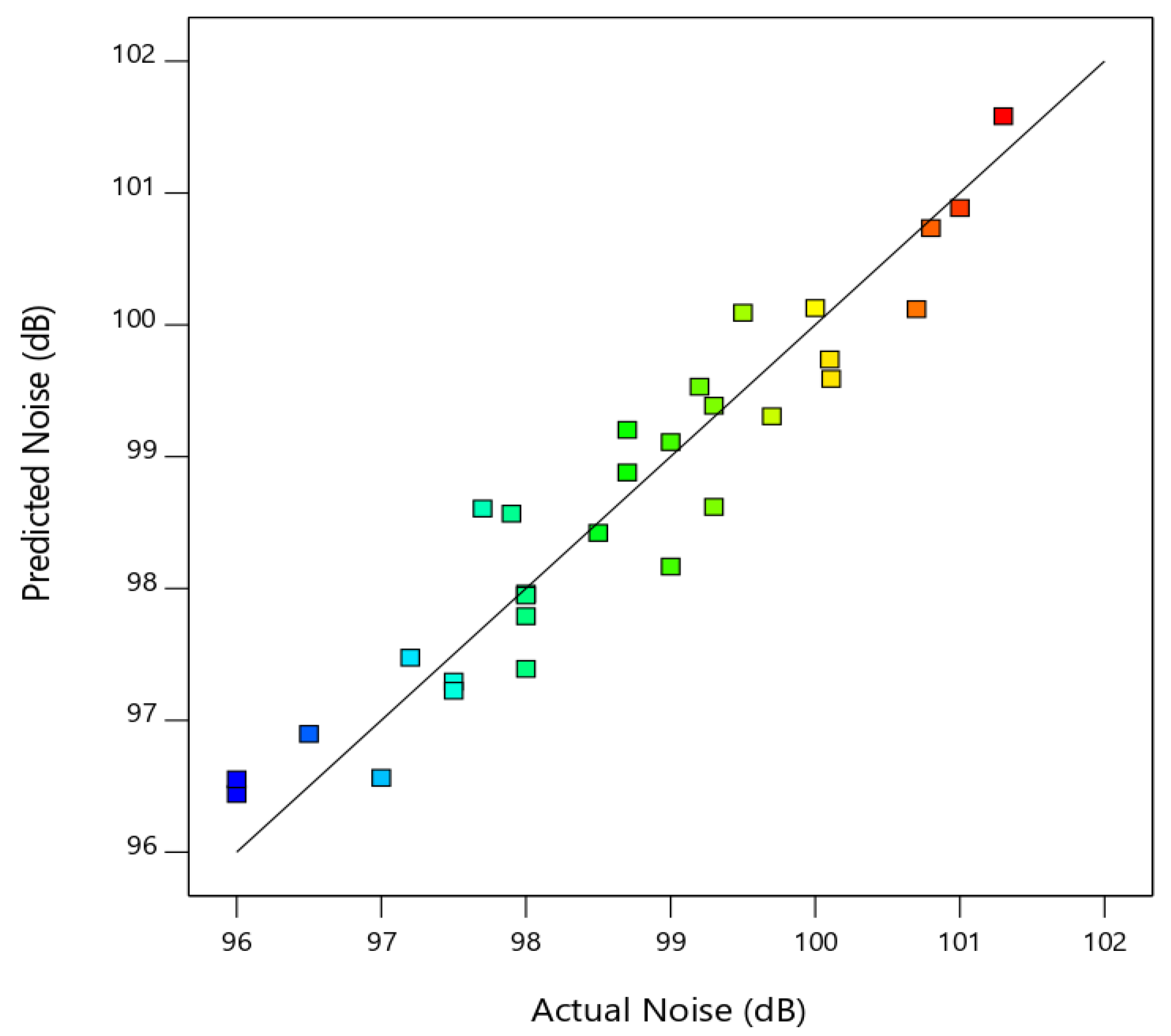
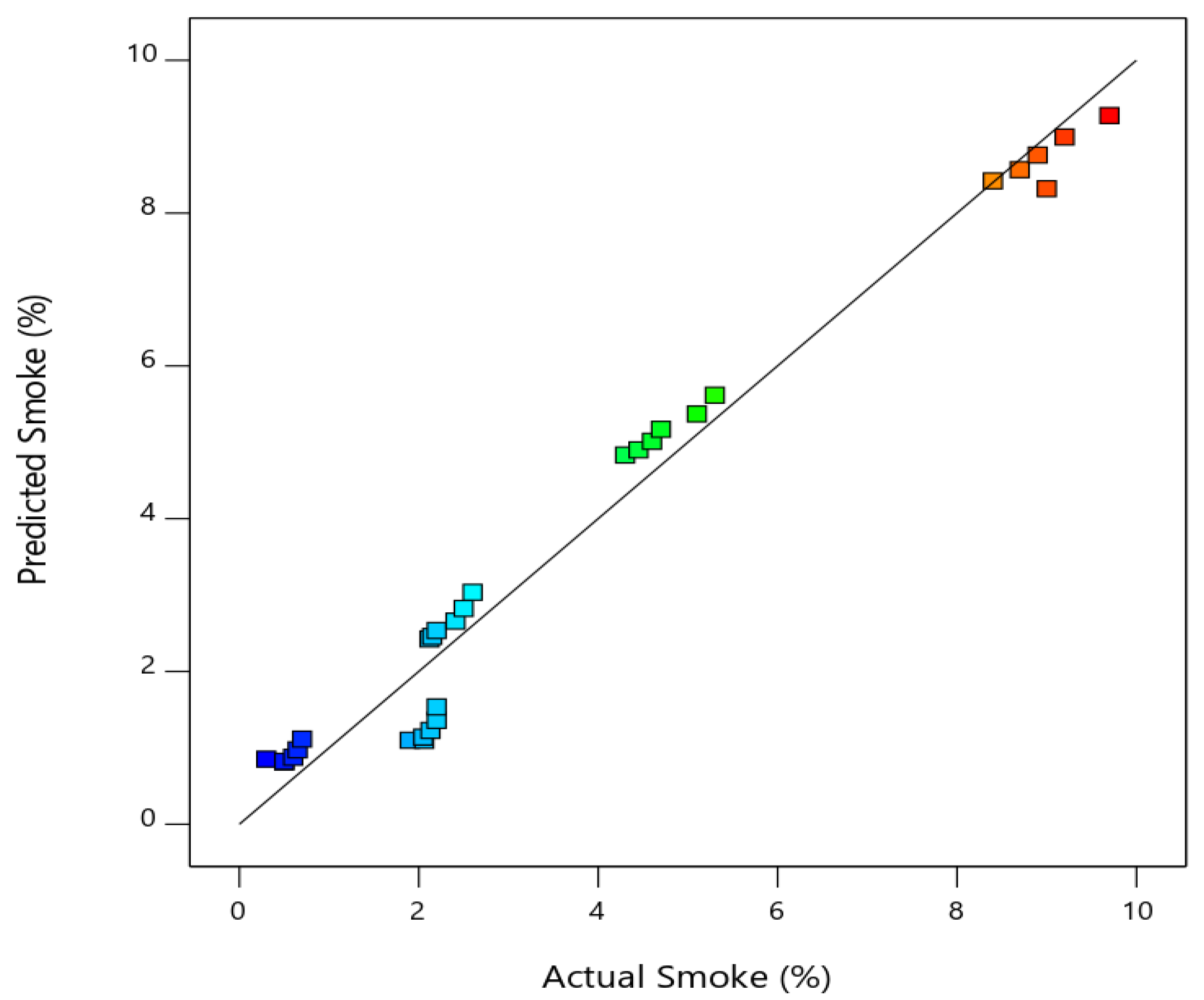
In addition to the performance and emission of an engine, factors of noise and smoke have also been considered. When the piston oscillates in the cylinder, it creates vibrations which consequently cause high noise levels. Moreover, when sudden ignition of fuel occurs inside the combustion chamber, it generates pressure waves that increase the intensity of the vibrations [42]. The smoke is produced as the result of a rich air–fuel mixture and lubricant burning in the combustion chamber [12].

Table 11. ANOVA results for noise.

Source	Sum of Squares	Df	Mean Square	F-Value	p-Value	PC (%)
Model	54.28	5	10.86	46.00	<0.0001	90.5503968
A-Load	7.91	1	7.91	33.50	<0.0001	13.18848462
B-HHO Concentration	44.54	1	44.54	188.68	<0.0001	74.2915545
AB	0.5103	1	0.5103	2.16	0.1545	0.851247727
A²	1.15	1	1.15	4.86	0.0373	1.915023405
B²	0.1823	1	0.1823	0.7723	0.3882	0.304086551
Residual	5.66	24	0.236			9.449603204
Cor Total	59.95	29

and

Table 12. ANOVA results for smoke.

Source	Sum of Squares	Df	Mean Square	F-Value	p-Value	PC (%)
Model	54.28	5	10.86	46.00	<0.0001	97.08694515
A-Load	7.91	1	7.91	33.50	<0.0001	87.15578304
B-HHO Concentration	44.54	1	44.54	188.68	<0.0001	0.496195224
AB	0.5103	1	0.5103	2.16	0.1545	0.080273582
A²	1.15	1	1.15	4.86	0.0373	9.319517418
B²	0.1823	1	0.1823	0.7723	0.3882	0.035175877
Residual	5.66	24	0.236			2.913054855
Cor Total	59.95	29

present the ANOVA results for noise and smoke. The quadratic models and study factors for both responses were significant. Variations in noise would be more due to HHO concentration rather than load, as shown by percentage contributions of 13.19% and 74.30%. Similarly, the smoke model unveils that both load and fuel amount have a significant impact on smoke produced. Moreover, a model R² value close to one (based on

Table 13. Coefficient of determination for noise.

Coefficient of Determination	Value
R2	0.9055
Adjusted R2	0.8858
Predicted R2	0.8527

and

Table 14. Coefficient of determination for smoke.

Coefficient of Determination	Value
R2	0.9709
Adjusted R2	0.9468
Predicted R2	0.9528

) and actual versus predicted diagnostic descriptions (Figure 10 and Figure 11) evidenced the accuracy of the selected models. Equations (5) and (6) give the second-order regression equations of noise and smoke.

Noise (dB) = 96.9203 − 0.0315619 × Load + 0.353839 × HHO Concentration + 0.0018 × Load × HHO Concentration + 0.000519577 ×Load² − 0.0078125 × HHO Concentration².

(5)

Smoke (%) = 1.77495 − 0.0799333 × Load − 0.0645821 × HHO Concentration − 0.00115714 ×Load × HHO Concentration + 0.00239947 × Load² + 0.0055625 × HHO Concentration².

(6)

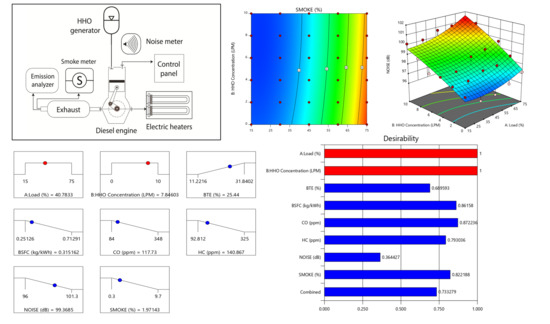
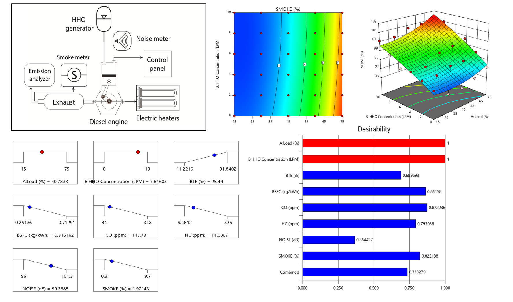
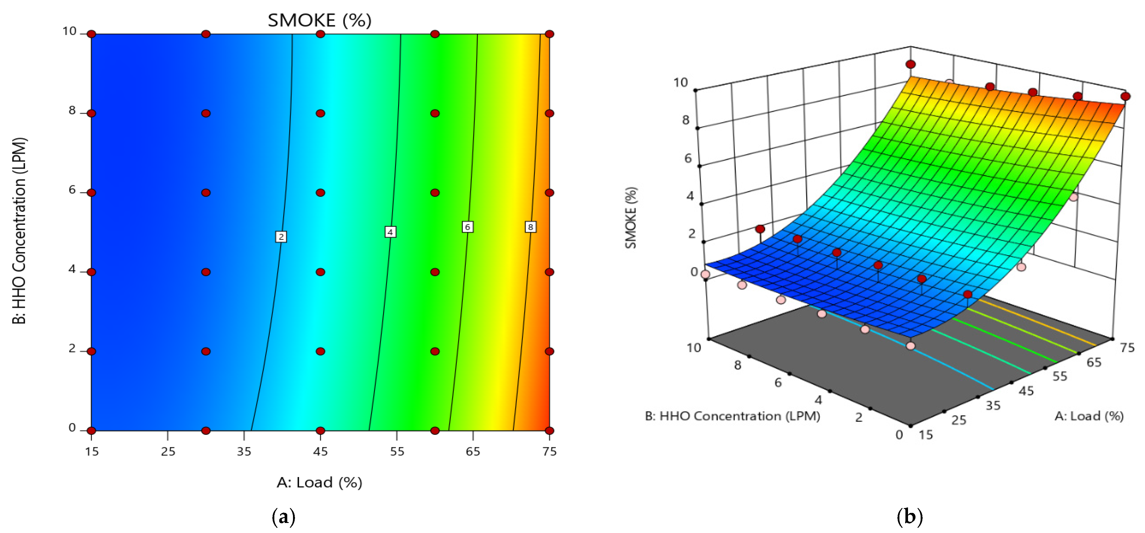
The effect of load and HHO on noise could be studied using the contour plots and response surface presented in Figure 12a,b. The red-colored region at the right top corner of Figure 12a indicates that, with the addition of HHO, the noise level increased and is at a maximum for 10 L/min HHO. The same trend could be seen more explicitly in Figure 12b where the response surface shows the gradual increase in noise level. The increased noise level with the addition of hydroxy gas could be apprehended by improved thermal efficiency and excessive combustion at high pressures inside the chamber [42,43]. The opacity is seen following a decreasing trend with a rise in fuel enrichment and load, as shown by Figure 13a,b. The contour plot and 3D response surface show that the least smoke is found for a blend of diesel with 10 L/min of HHO. The improved performance of an engine in terms of smoke emissions could be attributed to reduced HC emissions, high flame propagation, and high flame temperature of hydrogen [44].

4. RSM Based Optimization

Optimization is the study of maximizing output. An RSM-based optimization is a method to identify optimized conditions by maximizing or minimizing the study factors. In the current work, the emission and performance parameters of the engine are optimized using the numerical optimization feature of the Design Expert. In the optimization setup shown in

Table 15. Optimization setup.

Name	Goal	Lower Limit	Upper Limit	Lower Weight	Upper Weight	Importance
A: Load (%)	is in range	15	75	1	1	3
B: HHO Concentration (L/min)	is in range	0	10	1	1	3
BTE (%)	maximize	11.2216	31.8402	1	1	3
BSFC (kg/kWh)	minimize	0.25126	0.71291	1	1	3
Noise (dB)	minimize	96	101.3	1	1	3
HC (ppm)	minimize	92.812	325	1	1	3
Smoke (%)	minimize	0.3	9.7	1	1	3
CO (ppm)	minimize	84	348	1	1	3

, the goal of maximum was assigned to BTE only, while for smoke, noise, BSFC, CO, and HC the minimum criteria were selected. Moreover, the default in the range criterion for study factors was selected.

The engine operating conditions identified by optimization were 41% engine load and blend of diesel with 8 L/min HHO, both rounded to the nearest whole number. The response variables, corresponding to optimized operating conditions, were 25.44% BTE, 0.315 kg/kWh BSFC, 117.7 3 ppm of CO, 140.86 ppm of HC, 99.4 dB of noise, and smoke of 1.97%. The optimum gained values of study factors and response variables are shown by the red and blue dots in Figure 14. The experimentation and RSM models in the previous sections advocated the use of 10 L/min blended diesel for boosted performance and reduced emissions. However, at the same time, all the blend percentages were unfavorable for noise and therefore an optimum concentration of 8 L/min sounds reasonable.

The statistical identification of how optimization involved the overall responses could be studied through composite desirability (D). It is a unitless value in the range of 0–1, with 1 for the best and 0 for the worst case. In the current study, composite desirability is 0.733, which is a clear indication that the optimization settings have achieved favorable outcomes for all responses. The contour plot of desirability is shown in Figure 15. Moreover, the impact of individual responses on the overall setting could be assessed through the individual desirability (d) of each response, as shown by the bar graph in Figure 16. It is evident that d is largest for CO (0.877) and lowest for noise (0.364). The numerical values show that minimizing carbon monoxide emissions would have the greatest impact on the overall settings compared, and minimizing noise would impart the least impact to the setting as a whole.

5. Validation of RSM Results

The obtained RSM multi-optimization results were validated using experimentation. The engine was operated on the optimal values of load and HHO concentration and the responses were recorded. The absolute percentage error (APE) between the RSM predicted and experimentally obtained results was calculated as shown in

Table 16. Comparison of RSM and experimental values.

HHO Concentration (L/min)	Load (%)	Value	BTE (%)	BSFC kg/kWh	CO ppm	HC ppm	Noise dB	Smoke (%)
8	41	RSM Predicted	25.44	0.315	117.73	140.87	99.37	1.97
		Experimental	26.22	0.4	121	138.4	96.22	2
		APE	3.07	4.76	2.78	1.75	3.17	1.52

.

The APE shows that the developed RSM models and optimization results are accurate. The predicted results showed a reasonable agreement with the experimental results, with APE of all responses being below 5%. However, the maximum APE of 4.76% was evaluated for BSFC, which may be due to inefficient desirability resulting from manual recording during experimentation. Collectively, the predicted results of the developed models were efficient, which promised the simplification of complex performances with the least investment of time, effort and capital.

6. Conclusions

The purpose of the current investigation was to examine the impact of the blends of diesel with HHO on performance, noise, smoke and tailpipe emissions. Engine load and blend percentage of HHO were the varying factors. The following conclusions could be obtained from the research.

• ANOVA analysis of all the developed quadratic models indicated suitable fits.
• The 10 L/min HHO blended diesel proved valuable for improving performance, smoke, and for containing emissions.
• The noise increased for all the blended fuels and was maximum for 10 L/min HHO.
• The optimum blend flow rate among 0–10 L/min was 8 L/min for an engine load of 41%.
• Optimization revealed a composite desirability value of 0.733 with 25.44%, 0.315 kg/kWh, 117.73 ppm, 140.87 ppm, 99.37 dB, and 1.97% for BTE, BSFC, CO, HC, noise, and smoke respectively.
• In the optimization model, the most and least significant factors affecting desirability (D) were CO and noise, respectively.
• APE predicted that experimental results were below 5%.

The ANOVA and optimization results indicated the potential of hydroxy gas to be used as an alternative fuel in a CI engine. Thus, the use of HHO in blend percentages with diesel will help to save the stability of the Earth from deteriorating due to significantly reduced exhaust emissions compared to pure diesel. Moreover, the use of the RSM technique is beneficial and could save time and capital.

References

1. Höök, M.; Tang, X. Depletion of fossil fuels and anthropogenic climate change—A review. Energy Policy 2013, 52, 797–809. [Google Scholar] [CrossRef] [Green Version]
2. Abas, N.; Kalair, A.; Khan, N. Review of fossil fuels and future energy technologies. Futures 2015, 69, 31–49. [Google Scholar] [CrossRef]
3. Kverndokk, S. Depletion of Fossil Fuels and the Impact of Global Warming; Discussion Papers; Statistics Norway Research Department: Oslo, Norway, 1994.
4. Martins, F.; Felgueiras, C.; Smitkova, M.; Caetano, N. Analysis of fossil fuel energy consumption and environmental impacts in European countries. Energies 2019, 12, 964. [Google Scholar] [CrossRef] [Green Version]
5. Li, N.; Mu, H.; Li, H.; Gui, S. Diesel consumption of agriculture in China. Energies 2012, 5, 5126–5149. [Google Scholar] [CrossRef] [Green Version]
6. González-Marrero, R.M.; Lorenzo-Alegría, R.M.; Marrero, G.A. A dynamic model for road gasoline and diesel consumption: An application for Spanish regions. Int. J. Energy Econ. Policy 2012, 2, 201–209. [Google Scholar]
7. Agheli, L. Estimating the demand for diesel in agriculture sector of Iran. Int. J. Energy Econ. Policy 2015, 5, 660–667. [Google Scholar]
8. Nesamani, K.S. Estimation of automobile emissions and control strategies in India. Sci. Total Environ. 2010, 408, 1800–1811. [Google Scholar] [CrossRef] [PubMed]
9. Sequera, A.; Parthasarathy, R.; Gollahalli, S. Effect of Fuel Injection Timing in the Combustion of Biofuels in a Diesel Engine. In Proceedings of the 7th International Energy Conversion Engineering Conference, Denver, CO, USA, 2–5 August 2009. [Google Scholar]
10. Singh, P.; Chauhan, S.R.; Goel, V.; Gupta, A.K. Enhancing diesel engine performance and reducing emissions using binary biodiesel fuel blend. J. Energy Resour. Technol. 2020, 142, 01220. [Google Scholar] [CrossRef]
11. Castro, N.; Toledo, M.; Amador, G. An experimental investigation of the performance and emissions of a hydrogen-diesel dual fuel compression ignition internal combustion engine. Appl. Therm. Eng. 2019, 156, 660–667. [Google Scholar] [CrossRef]
12. Devarajan, Y. Experimental evaluation of combustion, emission and performance of research diesel engine fuelled Di-methyl-carbonate and biodiesel blends. Atmos. Pollut. Res. 2019, 10, 795–801. [Google Scholar] [CrossRef]
13. Elgarhi, I.; El-Kassaby, M.M.; Eldrainy, Y.A. Enhancing compression ignition engine performance using biodiesel/diesel blends and HHO gas. Int. J. Hydrogen Energy 2020, 45, 25409–25425. [Google Scholar] [CrossRef]
14. Hassan, Z.U.; Usman, M.; Asim, M.; Kazim, A.H.; Farooq, M.; Umair, M.; Imtiaz, M.U.; Asim, S.S. Use of diesel and emulsified diesel in CI engine: A comparative analysis of engine characteristics. Sci. Prog. 2021, 104, 368504211020930. [Google Scholar] [CrossRef] [PubMed]
15. Song, J.; Wang, G. An Experimental Study on Combustion and Performance of a Liquefied Natural Gas–Diesel Dual-Fuel Engine With Different Pilot Diesel Quantities. J. Therm. Sci. Eng. Appl. 2020, 12, 021011. [Google Scholar] [CrossRef]
16. Kemal, A.; Kahraman, N.; Çeper, B.A. Prediction of performance and emission parameters of an SI engine by using artificial neural networks. Isi Bilimi Tek. Derg. J. Therm. Sci. Technol. 2013, 33, 57–64. [Google Scholar]
17. Elkelawy, M.; Etaiw, S.E.-d.H.; Bastawissi, H.A.-E.; Marie, H.; Elbanna, A.; Panchal, H.; Sadasivuni, K.; Bhargav, H. Study of diesel-biodiesel blends combustion and emission characteristics in a CI engine by adding nanoparticles of Mn (II) supramolecular complex. Atmos. Pollut. Res. 2020, 11, 117–128. [Google Scholar] [CrossRef]
18. Arat, H.T.; Baltacioglu, M.K.; Özcanli, M.; Aydin, K. Effect of using Hydroxy—CNG fuel mixtures in a non-modified diesel engine by substitution of diesel fuel. Int. J. Hydrogen Energy 2016, 41, 8354–8363. [Google Scholar] [CrossRef]
19. Jakliński, P.; Czarnigowski, J. An experimental investigation of the impact of added HHO gas on automotive emissions under idle conditions. Int. J. Hydrogen Energy 2020, 45, 13119–13128. [Google Scholar] [CrossRef]
20. Kumar, V.; Gupta, D.; Kumar, N. Hydrogen use in internal combustion engine: A review. Int. J. Adv. Cult. Technol. 2015, 3, 87–99. [Google Scholar] [CrossRef]
21. Zohuri, B. Cryogenics and Liquid Hydrogen Storage. In Hydrogen Energy; Springer Nature Switzerland AG: Cham, Switzerland, 2019; pp. 121–139. [Google Scholar]
22. Kazim, A.H.; Khan, M.B.; Nazir, R.; Shabbir, A.; Abbasi, M.S.; Abdul Rab, H.; Shahid Qureishi, N. Effects of oxyhydrogen gas induction on the performance of a small-capacity diesel engine. Sci. Prog. 2020, 103, 36850420921685. [Google Scholar] [CrossRef]
23. Polverino, P.; D’Aniello, F.; Arsie, I.; Pianese, C. Study of the energetic needs for the on-board production of Oxy-Hydrogen as fuel additive in internal combustion engines. Energy Convers. Manag. 2019, 179, 114–131. [Google Scholar] [CrossRef]
24. Rajasekar, E.; Murugesan, A.; Subramanian, R.; Nedunchezhian, N. Review of NOx reduction technologies in CI engines fuelled with oxygenated biomass fuels. Renew. Sustain. Energy Rev. 2010, 14, 2113–2121. [Google Scholar] [CrossRef]
25. Sharma, P.K.; Sharma, D.; Soni, S.L.; Jhalani, A.; Singh, D.; Sharma, S. Characterization of the hydroxy fueled compression ignition engine under dual fuel mode: Experimental and numerical simulation. Int. J. Hydrog. Energy 2020, 45, 8067–8081. [Google Scholar] [CrossRef]
26. Subramanian, B.; Thangavel, V. Experimental investigations on performance, emission and combustion characteristics of Diesel-Hydrogen and Diesel-HHO gas in a Dual fuel CI engine. Int. J. Hydrog. Energy 2020, 45, 25479–25492. [Google Scholar] [CrossRef]
27. Usman, M.; Farooq, M.; Naqvi, M.; Saleem, M.W.; Hussain, J.; Naqvi, S.R.; Jahangir, S.; Jazim Usama, H.M.; Idrees, S.; Anukam, A. Use of gasoline, LPG and LPG-HHO blend in SI engine: A comparative performance for emission control and sustainable environment. Processes 2020, 8, 74. [Google Scholar] [CrossRef] [Green Version]
28. Usman, M.; Hayat, N.; Bhutta, M.M.A. SI Engine Fueled with Gasoline, CNG and CNG-HHO Blend: Comparative Evaluation of Performance, Emission and Lubrication Oil Deterioration. J. Therm. Sci. 2020, 30, 1199–1211. [Google Scholar] [CrossRef]
29. Baltacioglu, M.K.; Kenanoglu, R.; Aydın, K. HHO enrichment of bio-diesohol fuel blends in a single cylinder diesel engine. Int. J. Hydrog. Energy 2019, 44, 18993–19004. [Google Scholar] [CrossRef]
30. Kenanoğlu, R.; Baltacıoğlu, M.K.; Demir, M.H.; Özdemir, M.E. Performance & emission analysis of HHO enriched dual-fuelled diesel engine with artificial neural network prediction approaches. Int. J. Hydrog. Energy 2020, 45, 26357–26369. [Google Scholar]
31. Uslu, S. Optimization of diesel engine operating parameters fueled with palm oil-diesel blend: Comparative evaluation between response surface methodology (RSM) and artificial neural network (ANN). Fuel 2020, 276, 117990. [Google Scholar] [CrossRef]
32. Usman, M.; Naveed, A.; Saqib, S.; Hussain, J.; Tariq, M.K. Comparative assessment of lube oil, emission and performance of SI engine fueled with two different grades octane numbers. J. Chin. Inst. Eng. 2020, 43, 734–741. [Google Scholar] [CrossRef]
33. Xu, H.; Yin, B.; Liu, S.; Jia, H. Performance optimization of diesel engine fueled with diesel–jatropha curcas biodiesel blend using response surface methodology. J. Mech. Sci. Technol. 2017, 31, 4051–4059. [Google Scholar] [CrossRef]
34. Yadav, M.; Sawant, S. Effect of oxy-hydrogen blending with gasoline on vehicle performance parameters and optimization using response surface methodology. J. Chin. Inst. Eng. 2019, 42, 553–564. [Google Scholar] [CrossRef]
35. Aydın, M.; Uslu, S.; Çelik, M.B. Performance and emission prediction of a compression ignition engine fueled with biodiesel-diesel blends: A combined application of ANN and RSM based optimization. Fuel 2020, 269, 117472. [Google Scholar] [CrossRef]
36. Kehayov, D.; Komitov, G.; Ivanov, I. Influence of some factors on the gas flow produced by hho generator. Land Reclam. Earth Obs. Surv. Environ. Eng. 2019, 8, 188–191. [Google Scholar]
37. Nabil, T.; Dawood, M.M.K. Enabling efficient use of oxy-hydrogen gas (HHO) in selected engineering applications; transportation and sustainable power generation. J. Clean. Prod. 2019, 237, 117798. [Google Scholar] [CrossRef]
38. Al-Rousan, A.A.; Alkheder, S.; Musmar, S.e.A.; Al-Dabbas, M.A. Green transportation: Increasing fuel consumption efficiency through HHO gas injection in diesel vehicles. Int. J. Glob. Warm. 2018, 14, 372–384. [Google Scholar] [CrossRef]
39. Subramanian, B.; Ismail, S. Production and use of HHO gas in IC engines. Int. J. Hydrog. Energy 2018, 43, 7140–7154. [Google Scholar] [CrossRef]
40. Dahake, M.; Patil, S.; Patil, S. Effect of hydroxy gas addition on performance and emissions of diesel engine. Int. Res. J. Eng. Technol. 2016, 3, 756–760. [Google Scholar]
41. Momirlan, M.; Veziroglu, T.N. The properties of hydrogen as fuel tomorrow in sustainable energy system for a cleaner planet. Int. J. Hydrog. Energy 2005, 30, 795–802. [Google Scholar] [CrossRef]
42. Tüccar, G. Effect of hydroxy gas enrichment on vibration, noise and combustion characteristics of a diesel engine fueled with Foeniculum vulgare oil biodiesel and diesel fuel. Energy Sources Part A RecoveryUtil. Environ. Eff. 2018, 40, 1257–1265. [Google Scholar] [CrossRef]
43. Yıldırım, S.; Tosun, E.; Çalık, A.; Uluocak, İ.; Avşar, E. Artificial intelligence techniques for the vibration, noise, and emission characteristics of a hydrogen-enriched diesel engine. Energy Sources Part A RecoveryUtil. Environ. Eff. 2019, 41, 2194–2206. [Google Scholar] [CrossRef]
44. Rimkus, A.; Matijošius, J.; Bogdevičius, M.; Bereczky, Á.; Török, Á. An investigation of the efficiency of using O2 and H2 (hydrooxile gas-HHO) gas additives in a ci engine operating on diesel fuel and biodiesel. Energy 2018, 152, 640–651. [Google Scholar] [CrossRef]
Figure 1. Schematic of the experimental Setup.
Processes 09 01355 g001
Figure 2. (a) Contour plot and (b) response surface of BTE.
Processes 09 01355 g002
Figure 3. Comparison of actual and predicted BTE.
Processes 09 01355 g003
Figure 4. (a) Contour plot and (b) response surface of BSFC.
Processes 09 01355 g004
Figure 5. Comparison of actual and predicted BSFC.
Processes 09 01355 g005
Figure 6. Comparison of actual and predicted CO.
Processes 09 01355 g006
Figure 7. (a) Contour plot and (b) response surface of CO.
Processes 09 01355 g007
Figure 8. Comparison of actual and predicted HC.
Processes 09 01355 g008
Figure 9. (a) Contour plot and (b) response surface of HC.
Processes 09 01355 g009
Figure 10. Comparison of actual and predicted noise.
Processes 09 01355 g010
Figure 11. Comparison of actual and predicted smoke.
Processes 09 01355 g011
Figure 12. (a) Contour plot and (b) response surface of noise.
Processes 09 01355 g012
Figure 13. (a) Contour plot and (b) response surface of smoke.
Processes 09 01355 g013
Figure 14. Design expert identified optimum points.
Processes 09 01355 g014
Figure 15. Contour plot of desirability.
Processes 09 01355 g015
Figure 16. Desirability chart.
Processes 09 01355 g016