
Evaluation of One-Class Classifiers for Fault Detection: Mahalanobis Classifiers and the Mahalanobis–Taguchi System


1
ICT Digital Sector, SK Inc. C&C, Seongnam-si 13558, Korea
2
Department of Big Data Analytics, Kyung Hee University, Yongin-si 17104, Korea
3
Department of Industrial and Management Systems Engineering, Kyung Hee University, Yongin-si 17104, Korea
*
Author to whom correspondence should be addressed.
Processes 2021, 9(8), 1450; https://0-doi-org.brum.beds.ac.uk/10.3390/pr9081450
Submission received: 1 July 2021
/
Revised: 4 August 2021
/
Accepted: 16 August 2021
/
Published: 20 August 2021
(This article belongs to the Section Sustainable Processes)
Abstract
:Today, real-time fault detection and predictive maintenance based on sensor data are actively introduced in various areas such as manufacturing, aircraft, and power system monitoring. Many faults in motors or rotating machinery like industrial robots, aircraft engines, and wind turbines can be diagnosed by analyzing signal data such as vibration and noise. In this study, to detect failures based on vibration data, preprocessing was performed using signal processing techniques such as the Hamming window and the cepstrum transform. After that, 10 statistical condition indicators were extracted to train the machine learning models. Specifically, two types of Mahalanobis distance (MD)-based one-class classification methods, the MD classifier and the Mahalanobis–Taguchi system, were evaluated in detecting the faults of rotating machinery. Their performance for fault detection on rotating machinery was evaluated with different imbalanced ratios of data by comparing with binary classification models, which included classical versions and imbalanced classification versions of support vector machine and random forest algorithms. The experimental results showed the MD-based classifiers became more effective than binary classifiers in cases in which there were much fewer defect data than normal data, which is often common in the real-world industrial field.
1. Introduction
Recently, in manufacturing industry, there is much interest in smart manufacturing to improve productivity and competitiveness. The smart manufacturing is realized using advanced technologies such as the Internet of Things (IoT), artificial intelligence, and big data analysis [1]. Increasingly complex facilities in manufacturing systems need to be monitored and maintained in more sophisticated manners. To this end, the prognostics and health management (PHM) technology is capable of diagnosing or predicting faults by detecting or analyzing the condition of facilities using IoT, machine learning and big data analytics.
In particular, rotating machinery such as industrial motors, aircraft engines, and wind turbines are playing crucial roles in the automation of manufacturing systems. So, the fault detection of rotating machines has a decisive influence on system productivity. Many problems in rotary machines mainly come from the defects of bearing, gear boxes, or shaft deviation. The failure of a rotating machine that transmits power to various facilities results in great economic loss due to the performance degradation or shutdown of the system.
The rotating parts such as bearings often generate abnormal signal data if they have some problems; so, it is possible to diagnose the abnormal conditions by investigating the signal data. This signal data need appropriate preprocessing tasks based on various signal processing techniques, which make the signal data meaningful information that the user desires to analyze accurately and easily.
In this study, vibration data generated from rotating machines were preprocessed by applying appropriate signal processing techniques, and a fault-detection method was developed that can diagnose the abnormality of equipment parts in real time. The vibration data of normal and fault conditions were collected, and data standardization was then performed to compare with the same distribution. Thereafter, the Hamming window technique was applied to segment the vibration signal and a cepstrum technique was also adopted for enhancing the inherent characteristics by eliminating the existing noise. After preprocessing the data, 10 statistical condition indicators (SCIs), such as root mean squared (RMS) and peak-to-peak, were extracted to use for training the machine learning models. The extracted data were finally used to detect abnormal states by using the Mahalanobis distance (MD)-based one-class classification methods.
The MD-based one-class classification methods construct the Mahalanobis space (MS), represented by the MD using only the normal signal data, and then determine whether a new signal sample belongs to the MS or not. On the other hand, typical binary classification methods such as support vector machines (SVM) and random forest (RF) need both normal data and abnormal data to train the models for detecting abnormal condition of the system [2,3,4,5]. Unfortunately, in practical industrial systems, the amount of the fault data that can be collected is extremely small. For this reason, it is often difficult to apply typical two-class i.e., binary) classification techniques to construct the fault-detection models in real-life industrial systems. For that reason, in this paper we aimed to analyze the advantages and disadvantages of one-class classification techniques that consider data distribution. In particular, two MD-based classification methods were evaluated. First, the Mahalanobis distance classifier (MDC) used the Mahalanobis space based on MD to detect outliers and, moreover, the Mahalanobis–Taguchi System (MTS) adopted the Taguchi techniques to choose and use only key factors among all the variables.
The performances of the two MD-based classifiers were compared with binary classification methods and their imbalanced classification versions. The experimental results of performance comparison were investigated for the same test data set after training the models with different levels of imbalanced ratios (IRs) between normal and abnormal data in the training data set.
The remainder of this paper is structured as follows. In Section 2, we introduce related studies on the MD-based classification. In Section 3, we present the fault detection based on vibration data with the framework of the research. The signal processing methods, data preprocessing, and fault diagnosis classification models are also described. In Section 4, we compare the performance between one-class classifiers and binary classifiers according to different IRs of the same training data set. Finally, we conclude this paper with future work in Section 5.
2. Related Work
The MDC defines a normal group and constructs the MS using data from the normal group data [6]. A new sample is classified according to how far away it is from the pre-trained MS. Meanwhile, Taguchi proposed the MTS method by combining the MD-based classification method and the Taguchi method [7]. The Taguchi method is used to extract only effective variables with a large influence on MD estimation. The MTS method has been applied effectively to many fields such as diagnosis, pattern recognition, speech recognition and optimization [8,9].
The MTS technique is generally used for multivariate analysis. There are various studies comparing the performance between MTS and other multivariate analysis techniques. In large-scale samples, the performance of the techniques is similar, and there is a study in which the MTS technique is superior in small samples [10]. Moreover, the MTS still has the limitation of choosing optimal factors among all the variables [8,11], and so some studies integrated to MTS a feature selection such as genetic algorithm (GA) [12], particle swarm optimization [13], and ant colony optimization [14]. In particular, to improve the MTS process, Chen et al. developed two-stage Mahalanobis classification system (MCS) [15] and the integrated MCS (IMCS) [16]. In this paper, we focused on traditional MDC and MTS methods as one-class classifiers to compare their performance with binary classifiers according to the varying imbalanced ratio in detecting the fault of rotating machines based on the preprocessed vibration data.
Meanwhile, in the actual industry fields, there is little well-designed data that have proper quantities of positive samples and negative samples. Therefore, many researchers have studied to solve the imbalanced data set problem. According to [17], the number of published papers that study the imbalance learning is increasing since 2006. In 2016, 118 papers were published, and this is about 17 times the number of papers in 2006.
There are analytical studies to diagnose faults of rotating machines using the MD-based classification technique. Nader [18] used kernel whitening normalization and kernel principal component analysis (KPCA) to get the MD and showed that the techniques can be good choices when the training samples are small or the class is unique. Wei [19] suggested a novel kernel, Mahalanobis, ellipsoidal learning for one-class classification. Bartkowiak [20] used three methods, Parzen kernel density, mixture of Gaussians, and Support Vector Data Description (SVDD) after calculating MD, to find outliers for diagnosis of gearboxes.
3. Fault Detection Based on Vibration Data
3.1. Framework
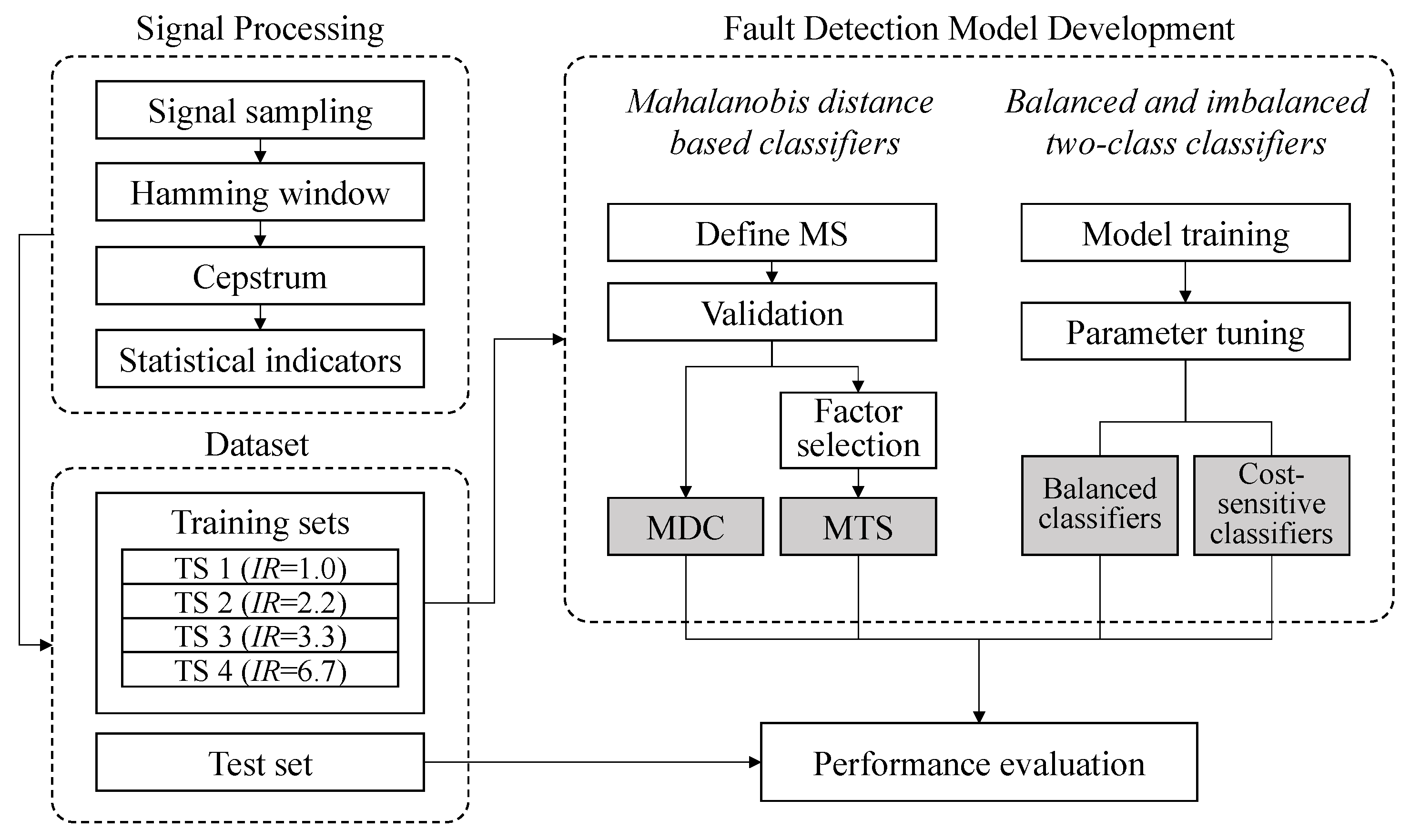
The procedure for developing a fault-detection model that can classify normal and abnormal data is shown in Figure 1. First, the vibration data of normal and abnormal states are collected for analysis. The collected vibration data are subjected to the windowing process. In this process, a continuous signal having a long length is divided into blocks by using the Hamming window function, and the values are set to values near 0 toward the boundary of the window frame. The original signal is then separated from the noise by the cepstrum transform process and the signal is denoised. In this research, 10 SCIs, such as mean, peak-to-peak, and RMS, were used to extract features for classification models. Those indicators are often used to represent the features from time series data in bearing fault-detection problems [21,22,23,24].
The preprocessed data were split into training and test sets to evaluate the MD-based classification methods. By using the training sets of preprocessed data, two MD-based classification models, MDC and MTS, were constructed as one-class classifiers. They were evaluated by comparing their accuracy with two representative binary classification methods, SVM and RF, and their imbalanced classification versions, cost-sensitive SVM and cost-sensitive RF. Finally, the performances of the developed models were compared in terms of several classification performance measures with the same test sets.
3.2. Data Description
In this study, we used the vibration signal data of the ball bearing provided by the Bearing Data Center of Case Western Reserve University [25]. It collected the vibration data using the accelerometer in the sensors attached to the rotating machine. The data set contained 12,000 digital signal values per second under the condition of RPM 1750. It consisted of 12,000 continuous vibration values, and the class consisted of a normal state and three abnormal states of system fault, ‘Ball’, ‘Inner race’, and ‘Outer race’.
In this experiment, we prepared four training data sets according to different imbalance ratios (IR) to compare the performance of one-class classifiers and binary classifiers by mimicking real-life industrial fields, where the fault data are extremely rare. The IR was used to evaluate the imbalance rate of the binary data, which were calculated as in Equation (1). The composition of the training data set according to IR is shown in Table 1. The test set consisted of 25 data including 10 normal and 15 abnormal data (five for each of three failure types).
3.3. Signal Processing and Data Preprocessing
In this subsection, we describe appropriate signal processing techniques. Signal processing means processing digitized signals by an algorithm for modifying or improving the signal for a specific purpose. In this research, the signal processing, such as standardization, Hamming window, cepstrum transformation, and statistical indicator extraction, were performed to be used for input of training fault-detection models.
3.3.1. Standardization
First, to compare the collected vibration data with the same distribution, standardization was performed using Equation (2). The is the vibration value at time in a signal data, is the standardized value of . The and mean the average and standard deviation of the vibration values respectively, and N is the number of vibration values.
3.3.2. Hamming Window and Cepstrum
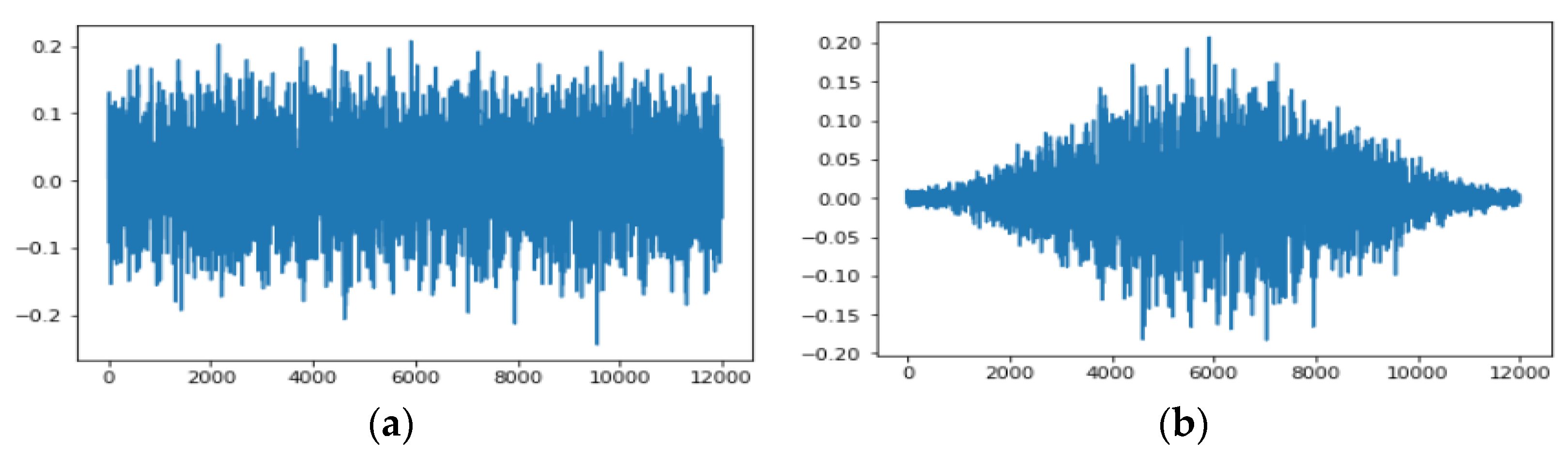
The vibration data used in this study were the arbitrarily divided data from a continuous vibration signal. There might have been a discontinuous part, that is, leakage error, which occurred because of arbitrary cutting of time series data. To remove the leakage, the Hamming window function was applied during Fast Fourier Transform (FFT). The window function made signal values near 0 toward the boundary of the window frame. By applying the Hamming window function, the signal periodicity can be ensured and a more accurate spectrum can be obtained from the result of the FFT. The window function is used when multiplying the original signal, as in Equation (3), where windowed signal is the multiplication of window function h(i) and input signal . Figure 2 shows the signal before applying the Hamming window function and the signal data after applying the Hamming window function.
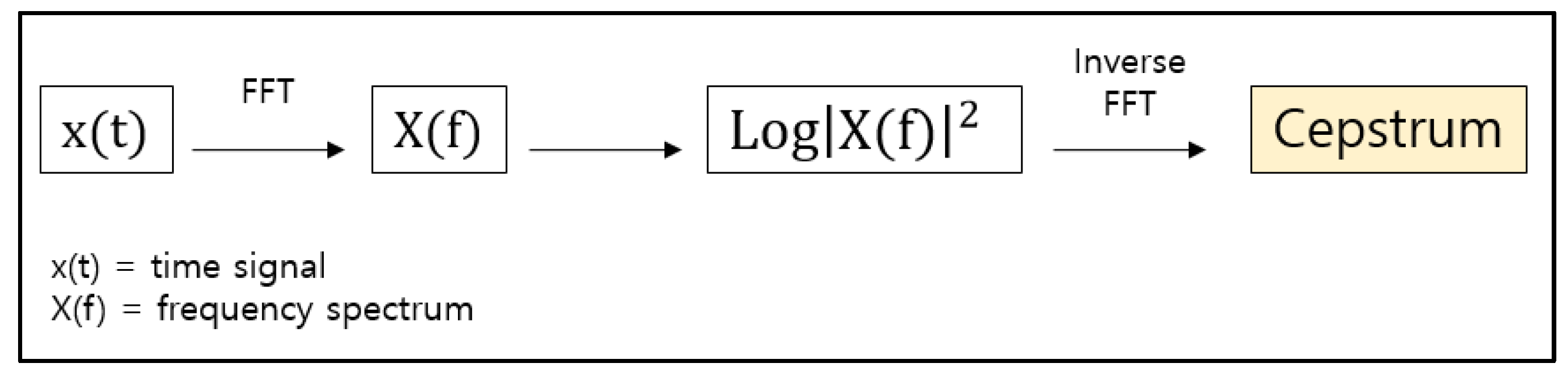
The cepstrum transform has the effect of obtaining an enhanced value of the original signal characteristic because it can extract the original signal, that is, the formant, from the noise, as depicted in Figure 3. The spectrum X(f), which is represented in frequency domain, was obtained by applying FFT to the time domain signal, x(t), then making it squared and giving it log function results in . Finally, inverse FFT was applied and we could get the result.
3.3.3. Extraction of Statistical Condition Indicators
SCIs are often used to effectively reflect the characteristics of the vibration data that have undergone signal processing [21,22,23,24]. Ten SCIs (mean, peak-to-peak, RMS, standard deviation, skewness, kurtosis, crest factor, shape factor, margin factor, and impulse factor) were extracted from the processed vibration data. Table 2 shows the formula of each indicator. Although we could detect the occurrence of faults by observing the changes in the statistical index values, we used them as the features for fault-detection modeling. The 10 SCIs were used as variables in the later classification modeling.
3.4. Fault Detection Using Mahalanobis Distance
To detect faults using the preprocessed data, we first used MDC, which is a MD-based classification technique. The technique uses MD as a comprehensive measure and constructs the MS using the MD of the normal signal group. The MD value of a signal will be used to distinguish normal and abnormal groups. In addition, the MTS method uses the Taguchi method to select only the important variables that have a major effect on the MD value and proceeds with the same procedure as MDC using only these important variables. The MTS method consists of four steps. Step 1 and step 2 are the classification procedure of MDC, and step 3 and step 4, including the Taguchi method, are the additional procedure for MTS.
3.4.1. Step 1: Constructing the MS with Normal Data
First, the normal and abnormal groups are distinguished from each other. MS is constructed using the normal data of the data set, which are denoted as shown in Table 3. The MS is a multi-dimensional unit space that is characterized with MD of the normal group. The MD is calculated through the three steps below.
- 1.
- Standardization of normal data
The mean of the pth feature, , and the standard deviation, , are first calculated from the feature data of the normal group, Xp = () for j = 1 … n. The pth feature value of the jth sample, , is standardized to as follows:
- 2.
- Calculation of the correlation matrix
The correlation matrix R for the standardized data of the normal group is obtained. The correlation coefficient between two variables, , in the correlation matrix R is calculated as follows.
- 3.
- Calculation of the MD of normal data
The MD of the jth normal data, , is calculated in Equation (7). The is often called the scaled Mahalanobis distance since it was divided by the number of variables, k.
where is the standardized vector of the jth variable and is the inverse of the correlation matrix. If the normal data are collected well, their MD values will have a value close to 1, since the average of is statistically 1. The MS constructed from the MD values in this way is called a unit space.
In this study, we prepared four training data sets with different IRs, as presented in Table 1, which, therefore, constructed different MS from their normal data. Table A1 in Appendix A shows the SCI values of 20 normal data in the training data that were used to construct its MS, and Table A2 in Appendix A shows the standardized data of the SCI values. From the standardized SCI values, the correlation matrix can be calculated as shown in Table 4. Finally, the final MD values of the normal data were calculated, as presented in Table 5a. The values were distributed well around 1. Note that the transformation to MD made the resulting distribution have the mean value of 1.
3.4.2. Step 2: MD Calculation of Abnormal Data and Validation of MS
To check the validity of the MS derived from Step 1, the MD values of abnormal data in the training data set were tested. Mean , standard deviation , and the correlation matrix R, which were obtained from the normal data in Step 1, were used again to calculate the MD of the abnormal data. If the MS is properly constructed from the normal data, the MD values of the abnormal data will have much larger values than the mean value of the normal group (i.e., 1).
The MD-based classifier for abnormality detection will decide a new data to abnormal if its MD is greater than a predefined threshold. The threshold can be set by comparing the MD values between normal data and abnormal data when they have enough abnormal data. However, it is not proper in one-class classification problems, assuming the small number of abnormal data. In this case, we set the MD threshold based on the chi-square value of a specific confidence interval (e.g., CI = 99%) because the MD was known to follow the chi-square distribution where the degree of freedom (df) is the number of variables [26].
- 1.
- Standardization of abnormal data
Abnormal data were prepared and denoted, as shown in Table 6. An abnormal data was standardized to by using mean and standard deviation of the normal data.
- 2.
- Calculation of the MD of abnormal data
The MD values of the abnormal data were calculated by using the correlation matrix R of the normal data. was the standardized vector of the jth variable for the abnormal data.
- 3.
- Validation of the MS
The MD values of the abnormal data are shown in Table 5b. The minimum value of the MD was 2269.5, and all the distance values were very far from the origin. Therefore, it can be said that the MS of the normal data was constructed successfully.
Now, the MS prepared in Step 2 can be used as the MDC classifier. Using the validated MS, MDC will classify a new data by comparing its MD with the specific threshold. Suppose that the threshold is set as the chi-square value = 23.2 of CI = 99% and df = 10 since the number of variables is 10. If the MD value of a new data is greater than the threshold, the data are classified to an abnormal state, and otherwise, to a normal state.
3.4.3. Step 3: Important Variable Selection (Taguchi Method of MTS)
In Steps 3 and 4, the MTS extracts key variables through the Taguchi method and carries out the classification procedure by calculating the MD values in the same manner as Steps 1 and 2.
In addition to the classification procedure of MDC, MTS removes the variables that have no or little effect on the MD values and chooses the key variables. By constructing MS using only the key variables, the system can be easily interpreted, and the classification performance can also be better. In MTS, the Taguchi method is adopted for selecting key variables [27]. The Taguchi method uses the signal-to-noise ratio (SN ratio) as a criterion for determining the degree of influence on the MD values. SN ratio in quality engineering is a measure for evaluating system robustness; however, in the MTS, it is used as a measure to select important parameters for pattern recognition. The formula of the SN ratio for the larger-the-better characteristics is as follows.
To calculate the SN ratio, the experiment was planned with an appropriate two-level orthogonal array. One should choose an orthogonal array that has a greater number of columns than the number of the variables used in the experiment. Since the number of variables used in this study was 10, we conducted the experiment with as the minimum two-level orthogonal array. Specifically, we used the Plackett–Burman , as presented in Table 7, so that the interaction effects among features could be uniformly diluted into all the columns of the arrays, as suggested by Dr. Taguchi [27].
Level 1 of the orthogonal array means that the corresponding variable was used, and level 2 means that the variable was not used. As shown in Table 7, the MD values of the normal and abnormal groups were calculated with 12 experimental conditions at each row. The SN ratio was then calculated using the SN ratio formula in Equation (10).
Next, we calculated the gain using the difference of average between the case where the variables were used and the case where the variables were not used. The gain of the SN ratio was calculated as follows.
Table 8 shows the results of calculating the gain of the SN ratio for each feature. If a feature has negative gain of SN ratio, the feature will be excluded from the feature set of MTS since the significance of the feature is low. If the gain of a feature is positive, the feature is selected as the key variable that has a significant effect on the MD value calculation. As shown in Table 8, seven features were selected as the key variables of MTS, excluding peak-to-peak, root mean squared, and crest factor features.
3.4.4. Step 4: Fault Detection Using MTS
Now, a new MS was constructed by using the seven features determined in Step 3, and then the classification procedure of Step 1 and Step 2 was conducted again. The threshold of determining the class was adjusted to the chi-square value, i.e., = 18.5 of CI = 99% and df = 7, because the number of selected important features was seven.
3.5. Fault Detection Based on Machine Learning Methods
In this subsection, we describe briefly how to classify normal and abnormal states by using binary classification machine learning methods. The models were developed by using both normal and abnormal data, and then they were used to distinguish whether a new data sample was a normal or abnormal state.
The four data sets shown in Table 1 were used for training two machine learning algorithms, SVM and RF, which are known to show convincible classification performance. In this study, as well as conventional SVM and RF, the imbalanced classification versions of SVM and RF were also tested because three of the four training data sets contained the small number of abnormal (fault) data, which is similar to real-life industrial field conditions. Specifically, cost-sensitive SVM (CS_SVM) and cost-sensitive RF (CS_RF) were used for the imbalanced classification algorithms. They adjust their class weights and make the training better. Parameter tuning of four machine learning methods was performed by using the grid search method under 3-fold cross validation.
4. Experiments
4.1. Classifiers and Datasets
To evaluate the proposed method, the classification performances using two MD-based one-class classification methods, MDC and MTS, were compared with those of four binary classification machine learning methods, which included classical versions of SVM and RF and their imbalanced classification versions, CS_SVM and CS_RF.
As shown in Table 1, the training data were constructed differently according to the imbalance ratio to investigate the change of binary classification methods. Note that MD and MS use only normal data for training because they are used as one-class classification methods. Twenty-five test data (10 normal and 15 abnormal) were used to compare the performance among all the classification models.
4.2. Experimental Results
As described in Section 3, one-class classifiers, MDC and MTS, classify a new sample based on the predefined threshold. We considered that the one-class classifiers do not know abnormal data and, so, the threshold was set according to confidence interval. In this research, the MDC used 10 features, and then the threshold was set to = 16.0 for CI = 90%, = 18.3 for CI = 95%, or = 23.2 for CI = 99%. Additionally, the MTS in this research used only seven important features and, therefore, the threshold was = 12.0 of CI = 90%, = 14.1 of CI = 95%, or = 18.5 of CI = 99%.
Table 9 shows the MD values of normal and abnormal data in test data set that were calculated by MDC and MTS. All normal data except for sample #7 were classified by MDC and MTS to normal because their MDs were less than the threshold. However, MDC misclassified sample #7 to abnormal because MD7 = 26.843 was a little greater than = 23.2.
The classification performances of MDC and MTS were compared with those of balanced and imbalanced binary classifiers of SVM and RF in terms of four measures such as accuracy, balanced accuracy, F-score, and G-mean. The last three measures are often used for imbalanced classification.
As shown in Table 10 and Figure 4, MTS had perfect accuracy, while MDC had the F-score of 0.968 and the G-mean 0.949 because the normal sample #7 was misclassified. Note that MTS and MDC always had the same performance regardless of any of the four training sets since they used only 20 normal data.
In the case of IR = 1.0, all of the four machine learning-based classifiers also showed perfect performance since there were enough abnormal data in the training data. However, as the number of abnormal data in training sets became smaller, which meant IR was higher, the overall classification performances turned lower. In the case of IR = 2.222 and IR = 3.333, CS_SVM showed similar performance to MDC and less than MTS, but SVM, RF, and CS_RF had lower performances. When IR became 6.667, all the binary classification methods had much lower performances than MDC and MTS.
Comparing two MD-based classifiers, MTS had better performance than MDC. Moreover, MTS can be said to be robust since it could be applied with smaller significant features in our experiments. So, the model can easily be interpreted with the small number of features in real-life industrial systems by using the important SCIs.
5. Conclusions and Future Work
In this study, we evaluated two MD-based one-class classification methods, MDC and MTS, for fault detection of rotating machines using vibration data. To use the vibration data for analysis, they were preprocessed by applying signal processing techniques such as the Hamming window and the cepstrum transformation. Moreover, 10 SCIs such as mean, standard deviation, peak-to-peak, and RMS were extracted and used as input variables for model training. To obtain meaningful results in the real-life industrial field where there are very few fault (abnormal) data compared with normal data, MDC and MTS were compared with the binary classification methods of training the data sets with different IRs.
We focused on one-class classification methods using MD because they do not need any abnormal data in training models. The two MD-based classifiers were compared with balanced and imbalanced binary classification algorithms such as SVM and RF. In the experiments, there was a tendency that the classification performances of the binary classification models were highly degraded as the number of abnormal data in the training set decreased. As a result, MDC and MTS showed much better performance than binary classifiers in the case of small amounts of abnormal training data.
The experiments are significant in that most working industrial systems in real fields rarely have fault data because they often stop the system before the occurrence of fault. Although the collection of fault data is possible, it needs a long time or high cost. This means that one-class classifiers are generally more useful in terms of cost, time, and effort if they can work with acceptable performance.
In addition, between MD-based classifiers, the MTS that selects only key variables through the Taguchi method can be useful in an actual operation environment since the small number of features are easily interpretable, as well as being fast and convenient to apply to the applications. In our experiment, MTS was robust enough to show better performance than MDC.
As future work, one can test many other signal processing techniques except for the Hamming window and the cepstrum transformation. The classification performance may be able to be improved by applying different signal processing techniques suited to the characteristics of data. In addition, some improved MTS methods such as MCS [15] and IMCS [16] have been developed, as described in Section 2. They can be evaluated with the traditional MD classifiers and the machine learning methods, as well. Finally, the performance may be able to be enhanced by applying recently developed deep learning algorithms and other parameter optimization techniques. From the viewpoint of the imbalanced data, one can use sampling-based techniques such as SMOTE [28] and ADASYN [29] in addition to applying cost-sensitive learning algorithms.
Author Contributions
Conceptualization, S.-G.K. and J.-Y.J.; methodology, S.-G.K. and J.-Y.J.; software, S.-G.K. and D.P.; validation, D.P. and J.-Y.J.; data curation, S.-G.K. and D.P.; writing—original draft preparation, S.-G.K.; writing—review and editing, J.-Y.J.; visualization, S.-G.K. and J.-Y.J.; supervision, J.-Y.J.; project administration, J.-Y.J.; funding acquisition, J.-Y.J. All authors have read and agreed to the published version of the manuscript.
Funding
This work was supported by the National Research Foundation of Korea (NRF) grants funded by the Korean government (MSIT) (Nos. 2017H1D8A2031138, 2019R1F1A1064125, and the Korea Institute for Advancement of Technology (KIAT) grant funded by the Korean Government (MOTIE) (Advanced Training Program for Smart Factory, No. N0002429).
Institutional Review Board Statement
Not applicable.
Informed Consent Statement
Not applicable.
Conflicts of Interest
The authors declare no conflict of interest.
Appendix A

Table A1.
SCI values extracted from the normal data in the training set.
| No. | X1 | X2 | X3 | X4 | X5 | X6 | X7 | X8 | X9 | X10 |
|---|---|---|---|---|---|---|---|---|---|---|
| 1 | 0.0022 | 0.1110 | 88.2268 | 8450.7533 | 11.0849 | 0.1110 | 99.8530 | 51.5367 | 35,304.5702 | 5146.0979 |
| 2 | 0.0022 | 0.1088 | 85.1839 | 7926.0778 | 10.6683 | 0.1088 | 98.0390 | 49.3359 | 33,338.4755 | 4836.8438 |
| 3 | 0.0022 | 0.1071 | 82.8757 | 7521.9721 | 10.3422 | 0.1071 | 96.5281 | 48.3374 | 31,608.3525 | 4665.9227 |
| 4 | 0.0022 | 0.1080 | 84.0284 | 7719.7090 | 10.5124 | 0.1081 | 97.2737 | 49.2069 | 32,280.4954 | 4786.5324 |
| 5 | 0.0022 | 0.1067 | 85.6983 | 8014.0618 | 10.4954 | 0.1067 | 98.3520 | 49.5043 | 32,362.5771 | 4868.8510 |
| 6 | 0.0021 | 0.1035 | 82.9297 | 7525.5047 | 9.9935 | 0.1035 | 96.5338 | 48.3207 | 30,518.9838 | 4664.5823 |
| 7 | 0.0022 | 0.1053 | 83.3340 | 7602.2303 | 10.2032 | 0.1054 | 96.8374 | 48.0261 | 30,964.2083 | 4650.7214 |
| 8 | 0.0022 | 0.1073 | 84.6176 | 7826.8295 | 10.4786 | 0.1073 | 97.6769 | 48.8701 | 32,159.0700 | 4773.4776 |
| 9 | 0.0022 | 0.1092 | 84.7386 | 7847.4618 | 10.6801 | 0.1093 | 97.7501 | 49.4621 | 33,158.9821 | 4834.9262 |
| 10 | 0.0022 | 0.1080 | 84.3215 | 7775.5606 | 10.5262 | 0.1080 | 97.4880 | 48.7086 | 31,886.4665 | 4748.5030 |
| 11 | 0.0022 | 0.1059 | 83.2398 | 7585.7523 | 10.2491 | 0.1059 | 96.7739 | 48.3551 | 31,415.7581 | 4679.5124 |
| 12 | 0.0022 | 0.1070 | 82.3364 | 7425.0616 | 10.2932 | 0.1071 | 96.1474 | 48.1050 | 31,339.2463 | 4625.1750 |
| 13 | 0.0022 | 0.1092 | 85.1613 | 7917.7262 | 10.7028 | 0.1092 | 98.0027 | 49.7627 | 32,885.3843 | 4876.8778 |
| 14 | 0.0022 | 0.1065 | 83.1586 | 7568.6743 | 10.3045 | 0.1066 | 96.7040 | 48.6730 | 31,968.7986 | 4706.8751 |
| 15 | 0.0022 | 0.1083 | 86.4437 | 8143.7671 | 10.7034 | 0.1083 | 98.8077 | 49.8898 | 33,144.6951 | 4929.4946 |
| 16 | 0.0022 | 0.1076 | 82.4792 | 7446.4014 | 10.3577 | 0.1076 | 96.2233 | 48.7696 | 31,740.4204 | 4692.7704 |
| 17 | 0.0022 | 0.1081 | 83.0734 | 7556.5331 | 10.4562 | 0.1082 | 96.6625 | 48.4062 | 31,988.0596 | 4679.0603 |
| 18 | 0.0022 | 0.1092 | 85.5365 | 7985.3777 | 10.7279 | 0.1092 | 98.2489 | 49.7376 | 33,212.4547 | 4886.6603 |
| 19 | 0.0022 | 0.1075 | 85.6612 | 8005.2812 | 10.5669 | 0.1075 | 98.3177 | 49.5240 | 32,216.5177 | 4869.0815 |
| 20 | 0.0022 | 0.1070 | 82.7790 | 7503.3918 | 10.3252 | 0.1070 | 96.4533 | 48.2209 | 31,383.3289 | 4651.0622 |
Table A2.
Standardized SCI values of the normal data in the training set.
| No. | Z1 | Z2 | Z3 | Z4 | Z5 | Z6 | Z7 | Z8 | Z9 | Z10 |
|---|---|---|---|---|---|---|---|---|---|---|
| 1 | −1.6567 | 2.1780 | 2.6094 | 2.5953 | 2.5595 | 2.1774 | 2.5130 | 3.0407 | 2.9609 | 2.9180 |
| 2 | 0.4734 | 0.7818 | 0.5919 | 0.6026 | 0.7863 | 0.7819 | 0.6287 | 0.3629 | 1.0589 | 0.4621 |
| 3 | 0.9235 | −0.2833 | −0.9385 | −0.9321 | −0.6018 | −0.2830 | −0.9406 | −0.8520 | −0.6148 | −0.8952 |
| 4 | 0.0854 | 0.3070 | −0.1742 | −0.1812 | 0.1225 | 0.3070 | −0.1662 | 0.2059 | 0.0355 | 0.0626 |
| 5 | −1.5919 | −0.5556 | 0.9329 | 0.9368 | 0.0501 | −0.5561 | 0.9539 | 0.5679 | 0.1149 | 0.7163 |
| 6 | −2.1366 | −2.5826 | −0.9027 | −0.9187 | −2.0860 | −2.5831 | −0.9347 | −0.8723 | −1.6686 | −0.9058 |
| 7 | −0.0113 | −1.4129 | −0.6346 | −0.6273 | −1.1934 | −1.4128 | −0.6194 | −1.2308 | −1.2379 | −1.0159 |
| 8 | 0.0416 | −0.1961 | 0.2164 | 0.2257 | −0.0211 | −0.1961 | 0.2527 | −0.2039 | −0.0820 | −0.0411 |
| 9 | 0.6099 | 1.0627 | 0.2966 | 0.3040 | 0.8364 | 1.0628 | 0.3287 | 0.5165 | 0.8853 | 0.4469 |
| 10 | 0.9320 | 0.2460 | 0.0201 | 0.0310 | 0.1815 | 0.2463 | 0.0564 | −0.4004 | −0.3457 | −0.2394 |
| 11 | −0.1638 | −1.0676 | −0.6971 | −0.6899 | −0.9981 | −1.0676 | −0.6853 | −0.8305 | −0.8011 | −0.7873 |
| 12 | 1.2926 | −0.3375 | −1.2961 | −1.3002 | −0.8102 | −0.3371 | −1.3360 | −1.1347 | −0.8751 | −1.2188 |
| 13 | 0.0177 | 1.0312 | 0.5769 | 0.5709 | 0.9331 | 1.0311 | 0.5911 | 0.8822 | 0.6206 | 0.7800 |
| 14 | −0.2039 | −0.6550 | −0.7509 | −0.7548 | −0.7625 | −0.6550 | −0.7579 | −0.4436 | −0.2661 | −0.5700 |
| 15 | −0.9441 | 0.4700 | 1.4272 | 1.4294 | 0.9357 | 0.4696 | 1.4272 | 1.0369 | 0.8715 | 1.1979 |
| 16 | 0.5359 | 0.0347 | −1.2014 | −1.2192 | −0.5360 | 0.0349 | −1.2573 | −0.3261 | −0.4870 | −0.6820 |
| 17 | 1.6720 | 0.3712 | −0.8074 | −0.8009 | −0.1168 | 0.3717 | −0.8010 | −0.7683 | −0.2474 | −0.7909 |
| 18 | 0.0483 | 1.0196 | 0.8257 | 0.8278 | 1.0399 | 1.0195 | 0.8468 | 0.8516 | 0.9370 | 0.8577 |
| 19 | −0.9893 | −0.0694 | 0.9083 | 0.9034 | 0.3547 | −0.0697 | 0.9182 | 0.5917 | −0.0264 | 0.7181 |
| 20 | 1.0654 | −0.3423 | −1.0026 | −1.0027 | −0.6739 | −0.3419 | −1.0183 | −0.9938 | −0.8324 | −1.0132 |
References
- Lee, S.H.; Yoon, B.D. Industry 4.0 and direction of failure prediction and health management technology (PHM). Trans. Korean Soc. Noise Vibr. Eng. 2015, 25, 22–28. [Google Scholar]
- Park, D.; Kim, S.; An, Y.; Jung, J.-Y. LiReD: A light-weight real-time fault detection system for edge computing using LSTM recurrent neural networks. Sensors 2018, 18, 2110. [Google Scholar] [CrossRef] [Green Version]
- Park, Y.-J.; Fan, S.-K.; Hsu, C.-Y. A review on fault detection and process diagnostics in industrial processes. Processes 2020, 8, 1123. [Google Scholar] [CrossRef]
- Fan, S.-K.S.; Hsu, C.-Y.; Tsai, D.-M.; He, F.; Cheng, C.-C. Data-driven approach for fault detection and diagnostic in semiconductor manufacturing. IEEE Trans. Autom. Sci. Eng. 2020, 17, 1925–1936. [Google Scholar]
- Lv, Q.; Yu, X.; Ma, H.; Ye, J.; Wu, W.; Wang, X. Applications of machine learning to reciprocating compressor fault diagnosis: A review. Processes 2021, 9, 909. [Google Scholar] [CrossRef]
- Xiang, S.; Nie, F.; Zhang, C. Learning a Mahalanobis distance metric for data clustering and classification. Pattern Recognit. 2008, 41, 3600–3612. [Google Scholar] [CrossRef]
- Taguchi, G.; Jugulum, R. The Mahalanobis Taguchi Strategy: A Pattern Technology System; John Wiley and Sons: Hoboken, NJ, USA, 2002. [Google Scholar]
- Woodall, W.H.; Koudelik, R.; Tsui, K.L.; Kim, S.B.; Stoumbos, Z.G.; Carvounis, C.P. A review and analysis of the Mahalanobis—Taguchi system. Technometrics 2003, 45, 1–15. [Google Scholar] [CrossRef]
- Cheng, L.; Yaghoubi, V.; van Paepegem, W.; Kersemans, M. On the influence of reference Mahalanobis distance space for quality classification of complex metal parts using vibrations. Appl. Sci. 2020, 10, 8620. [Google Scholar] [CrossRef]
- Wang, H.C.; Chiu, C.C.; Su, C.T. Data classification using the Mahalanobis Taguchi system. J. Chin. Inst. Ind. Eng. 2004, 21, 606–618. [Google Scholar] [CrossRef]
- Pal, A.; Maiti, J. Development of a hybrid methodology for dimensionality reduction in Mahalanobis–Taguchi system using Mahalanobis distance and binary particle swarm optimization. Expert Syst. Appl. 2010, 37, 1286–1293. [Google Scholar] [CrossRef]
- ReséNdiz, E.; Rull-Flores, C.A. Mahalanobis–Taguchi system applied to variable selection in automotive pedals components using Gompertz binary particle swarm optimization. Expert Syst. Appl. 2013, 40, 2361–2365. [Google Scholar] [CrossRef]
- Reséndiz, E.; Moncayo-Martínez, L.A.; Solís, G. Binary ant colony optimization applied to variable screening in the Mahalanobis-Taguchi system. Expert Syst. Appl. 2013, 40, 634–637. [Google Scholar] [CrossRef]
- El-Banna, M. A novel approach for classifying imbalance welding data: Mahalanobis genetic algorithm (MGA). Int. J. Adv. Manuf. Technol. 2015, 77, 407–425. [Google Scholar] [CrossRef]
- Cheng, L.; Yaghoubi, V.; van Paepegem, W.; Kersemans, M. Mahalanobis classification system (MCS) integrated with binary particle swarm optimization for robust quality classification of complex metallic turbine blades. Mech. Syst. Signal Process. 2021, 146, 107060. [Google Scholar] [CrossRef]
- Cheng, L.; Yaghoubi, V.; van Paepegem, W.; Kersemans, M. Quality inspection of complex-shaped metal parts by vibrations and an integrated Mahalanobis classification system. Struct. Health Monit. 2020, in press. [Google Scholar] [CrossRef]
- Haixiang, G.; Yijing, L.; Shang, J.; Mingyun, G.; Yuanyue, H.; Bing, G. Learning from class-imbalanced data: Review of methods and applications. Expert Syst. Appl. 2017, 73, 220–239. [Google Scholar] [CrossRef]
- Nader, P.; Honeine, P.; Beauseroy, P. Mahalanobis-based one-class classification. In Proceedings of the 2014 IEEE International Workshop on Machine Learning for Signal Processing (MLSP), Reims, France, 21–24 September 2014; pp. 1–6. [Google Scholar]
- Wei, X.K.; Huang, G.B.; Li, Y.H. Mahalanobis ellipsoidal learning machine for one class classification. In Proceedings of the 2007 International Conference on Machine Learning and Cybernetics, Hong Kong, China, 19–22 August 2007; Volume 6, pp. 3528–3533. [Google Scholar]
- Bartkowiak, A.; Zimroz, R. Outliers analysis and one class classification approach for planetary gearbox diagnosis. J. Phys. Conf. Ser. 2011, 305, 012031. [Google Scholar] [CrossRef]
- Wang, Z.; Wang, Z.; Tao, L.; Ma, J. Fault diagnosis for bearing based on Mahalanobis-Taguchi system. In Proceedings of the IEEE 2012 Prognostics and System Health Management Conference (PHM-2012 Beijing), Beijing, China, 23–25 May 2012; pp. 1–5. [Google Scholar]
- Wang, X.; Zheng, Y.; Zhao, Z.; Wang, J. Bearing fault diagnosis based on statistical locally linear embedding. Sensors 2015, 15, 16225–16247. [Google Scholar] [CrossRef]
- Hui, K.H.; Ooi, C.S.; Lim, M.H.; Leong, M.S.; Al-Obaidi, S.M. An improved wrapper-based feature selection method for machinery fault diagnosis. PLoS ONE 2017, 12, e0189143. [Google Scholar] [CrossRef] [Green Version]
- Cao, R.; Yuan, J. Selection strategy of vibration feature target under centrifugal pumps cavitation. Appl. Sci. 2020, 10, 8190. [Google Scholar] [CrossRef]
- Loparo, K.A. Bearings Vibration Data Set. The Case Western Reserve University Bearing Data Center. Available online: https://csegroups.case.edu/bearingdatacenter/ (accessed on 1 July 2021).
- Brereton, R.G. The chi squared and multinormal distributions. J. Chemom. 2015, 29, 9–12. [Google Scholar] [CrossRef]
- Mori, T. Appendix D–Q&A: The MT (Mahalanobis-Taguchi) System and Pattern Recognition. In Taguchi Methods: Benefits, Impacts, Mathematics, Statistics, and Applications; Mori, T., Ed.; ASME Press: New York, NY, USA, 2011; pp. 1035–1036. [Google Scholar]
- Chawla, N.V.; Bowyer, K.W.; Hall, L.O.; Kegelmeyer, W.P. SMOTE: Synthetic minority over-sampling technique. J. Artif. Intell. Res. 2002, 16, 321–357. [Google Scholar] [CrossRef]
- He, H.; Bai, Y.; Garcia, E.A.; Li, S. ADASYN: Adaptive synthetic sampling approach for imbalanced learning. In Proceedings of the 2008 IEEE World Congress On Computational Intelligence, Hong Kong, China, 1–6 June 2008; pp. 1322–1328. [Google Scholar]
Figure 1.
Procedure for fault-detection evaluation in this research.

Figure 2.
The vibration data (a) before and (b) after applying the Hamming window function.

Figure 3.
Cepstrum transformation process.

Figure 4.
Performance comparison among classifiers according to IRs. (a) F-score; (b) G-mean.

Table 1.
Data set configuration according to the imbalance ratio (IR). MDC and MTS use only normal data for training, while binary classification methods use both normal and abnormal data.
Table 1.
Data set configuration according to the imbalance ratio (IR). MDC and MTS use only normal data for training, while binary classification methods use both normal and abnormal data.
| Dataset | IR | # of Normal | # of Abnormal (Fault Types) | |
|---|---|---|---|---|
| Training Set | TS 1 | 1.000 | 20 | 20 (Ball 7, Inner 7, Outer 6) |
| TS 2 | 2.222 | 9 (Ball 3, Inner 3, Outer 3) | ||
| TS 3 | 3.333 | 6 (Ball 2, Inner 2, Outer 2) | ||
| TS 4 | 6.667 | 3 (Ball 1, Inner 1, Outer 1) | ||
| Test Set | 0.667 | 10 | 15 (Ball 5, Inner 5, Outer 5) | |
Table 2.
List of statistical condition indicators (SCIs).
| Indicator | Formula | Indicator | Formula |
|---|---|---|---|
| mean | root mean squared | ||
| standard deviation | crest factor | ||
| skewness | shape factor | ||
| kurtosis | margin factor | ||
| peak-to-peak | impulse factor |
Table 3.
Data schema of normal data.
| No. | X1 | X2 | X3 | X4 | … | Xk |
|---|---|---|---|---|---|---|
| … | ||||||
| 1 | … | |||||
| 2 | … | |||||
| 3 | … | |||||
| … | … | … | … | … | … | … |
| n | … | |||||
| mean | …. | |||||
| std. | … |
Table 4.
Correlation matrix between standardized SCI for the normal data in training set.
| No. | Z1 | Z2 | Z3 | Z4 | Z5 | Z6 | Z7 | Z8 | Z9 | Z10 |
|---|---|---|---|---|---|---|---|---|---|---|
| Z1 | 1.0000 | 0.1827 | −0.5465 | −0.5428 | −0.1220 | 0.1830 | −0.5381 | −0.4997 | −0.2303 | −0.5233 |
| Z2 | 0.1827 | 1.0000 | 0.6533 | 0.6536 | 0.9413 | 1.0000 | 0.6510 | 0.7603 | 0.8918 | 0.7319 |
| Z3 | −0.5465 | 0.6533 | 1.0000 | 1.0000 | 0.8704 | 0.6531 | 0.9994 | 0.9366 | 0.8712 | 0.9758 |
| Z4 | −0.5428 | 0.6536 | 1.0000 | 1.0000 | 0.8707 | 0.6534 | 0.9996 | 0.9345 | 0.8708 | 0.9745 |
| Z5 | −0.1220 | 0.9413 | 0.8704 | 0.8707 | 1.0000 | 0.9412 | 0.8690 | 0.9098 | 0.9675 | 0.9096 |
| Z6 | 0.1830 | 1.0000 | 0.6531 | 0.6534 | 0.9412 | 1.0000 | 0.6508 | 0.7601 | 0.8917 | 0.7317 |
| Z7 | −0.5381 | 0.6510 | 0.9994 | 0.9996 | 0.8690 | 0.6508 | 1.0000 | 0.9288 | 0.8662 | 0.9708 |
| Z8 | −0.4997 | 0.7603 | 0.9366 | 0.9345 | 0.9098 | 0.7601 | 0.9288 | 1.0000 | 0.9381 | 0.9905 |
| Z9 | −0.2303 | 0.8918 | 0.8712 | 0.8708 | 0.9675 | 0.8917 | 0.8662 | 0.9381 | 1.0000 | 0.9274 |
| Z10 | −0.5233 | 0.7319 | 0.9758 | 0.9745 | 0.9096 | 0.7317 | 0.9708 | 0.9905 | 0.9274 | 1.0000 |
Table 5.
Mahalanobis distances of training data.
| (a) MD values of 20 normal data. | ||||||||||
| j | 1 | 2 | 3 | 4 | 5 | 6 | 7 | 8 | 9 | 10 |
| MDj | 1.880 | 1.145 | 0.672 | 0.644 | 1.280 | 1.624 | 1.694 | 0.311 | 0.852 | 1.548 |
| j | 11 | 12 | 13 | 14 | 15 | 16 | 17 | 18 | 19 | 20 |
| MDj | 0.644 | 0.932 | 0.833 | 0.984 | 1.042 | 1.759 | 0.529 | 0.466 | 0.801 | 0.360 |
| (b) MD values of 20 abnormal data. | ||||||||||
| j | 1 | 2 | 3 | 4 | 5 | 6 | 7 | 8 | 9 | 10 |
| MDj | 36,679.5 | 6969.2 | 7641.3 | 1,423,858.3 | 2269.5 | 175,239.4 | 444,333.3 | 21,216.3 | 759,203 | 10,207.1 |
| j | 11 | 12 | 13 | 14 | 15 | 16 | 17 | 18 | 19 | 20 |
| MDj | 112,695.9 | 97,902.2 | 384,358.2 | 50,910.3 | 68,695.8 | 39,944.1 | 168,569.9 | 33,557.8 | 37,939.4 | 151,305.5 |
Table 6.
Data schema of abnormal group data.
| No. | X1 | X2 | X3 | X4 | … | Xk |
|---|---|---|---|---|---|---|
| … | ||||||
| 1 | … | |||||
| 2 | … | |||||
| 3 | … | |||||
| … | … | … | … | … | … | … |
| n | … |
Table 7.
SN ratios with .
| No. | X1 | X2 | X3 | X4 | X5 | X6 | X7 | X8 | X9 | X10 | X11 | SNR |
|---|---|---|---|---|---|---|---|---|---|---|---|---|
| dummy | ||||||||||||
| 1 | 1 | 1 | 1 | 1 | 1 | 1 | 1 | 1 | 1 | 1 | 1 | −1.124 |
| 2 | 2 | 1 | 2 | 1 | 1 | 1 | 2 | 2 | 2 | 1 | 2 | −1.929 |
| 3 | 2 | 2 | 1 | 2 | 1 | 1 | 1 | 2 | 2 | 2 | 1 | −3.201 |
| 4 | 1 | 2 | 2 | 1 | 2 | 1 | 1 | 1 | 2 | 2 | 2 | −1.793 |
| 5 | 2 | 1 | 2 | 2 | 1 | 2 | 1 | 1 | 1 | 2 | 2 | −2.190 |
| 6 | 2 | 2 | 1 | 2 | 2 | 1 | 2 | 1 | 1 | 1 | 2 | −1.659 |
| 7 | 2 | 2 | 2 | 1 | 2 | 2 | 1 | 2 | 1 | 1 | 1 | −2.119 |
| 8 | 1 | 2 | 2 | 2 | 1 | 2 | 2 | 1 | 2 | 1 | 1 | −1.808 |
| 9 | 1 | 1 | 2 | 2 | 2 | 1 | 2 | 2 | 1 | 2 | 1 | −2.178 |
| 10 | 1 | 1 | 1 | 2 | 2 | 2 | 1 | 2 | 2 | 1 | 2 | −1.487 |
| 11 | 2 | 1 | 1 | 1 | 2 | 2 | 2 | 1 | 2 | 2 | 1 | −1.631 |
| 12 | 1 | 2 | 1 | 1 | 1 | 2 | 2 | 2 | 1 | 2 | 2 | −1.358 |
Table 8.
Gain of SN ratio for each feature.
| Level | X1 | X2 | X3 | X4 | X5 | X6 | X7 | X8 | X9 | X10 |
|---|---|---|---|---|---|---|---|---|---|---|
| L1 | −1.625 | −1.757 | −1.743 | −1.659 | −1.935 | −1.981 | −1.986 | −1.701 | −1.771 | −1.688 |
| L2 | −2.122 | −1.990 | −2.003 | −2.087 | −1.811 | −1.765 | −1.761 | −2.046 | −1.975 | −2.058 |
| Gain | 0.497 | 0.233 | 0.260 | 0.428 | −0.124 | −0.216 | −0.225 | 0.345 | 0.204 | 0.370 |
| +/– | + | + | + | + | – | – | – | + | + | + |
Table 9.
Mahalanobis distances of test data.
| (a) MD values of 10 normal data of test data. | |||||||||||
| j | Classifier | 1 | 2 | 3 | 4 | 5 | 6 | 7 | 8 | 9 | 10 |
| MDj | MDC | 4.569 | 1.712 | 3.498 | 2.282 | 1.165 | 1.130 | 26.843 | 1.667 | 1.020 | 1.611 |
| MTS | 2.437 | 1.250 | 2.268 | 2.537 | 0.990 | 0.574 | 8.030 | 0.824 | 1.225 | 1.670 | |
| (b) MD values of 15 abnormal data of test data. | |||||||||||
| j | Classifier | 1 | 2 | 3 | 4 | 5 | 6 | 7 | 8 | ||
| MDj | MDC | 722,066.6 | 33,487.3 | 636,322.9 | 21,249.4 | 1,099,766.7 | 38,561.8 | 115,765.9 | 24,139.0 | ||
| MTS | 79,053.5 | 2804.4 | 85,754.0 | 1707.4 | 105,073.8 | 9267.4 | 7808.5 | 2743.2 | |||
| j | Classifier | 9 | 10 | 11 | 12 | 13 | 14 | 15 | |||
| MDj | MDC | 24,254.3 | 21,776.8 | 254,774.4 | 268,589.7 | 2,895,042.0 | 865,706.8 | 1,994,251.8 | |||
| MTS | 3591.8 | 1424.0 | 20,894.4 | 19,864.0 | 244,433.8 | 107,917.9 | 170,577.2 | ||||
Table 10.
Performance for the test set of classifiers trained with different training sets.
| Training Set | IR (# Normal: # Abnormal) | Classifier | Parameter | Accuracy | Balanced Accuracy | Recall | Precision | F-Score | G-Mean |
|---|---|---|---|---|---|---|---|---|---|
| Any set | ∞ (20:0) | MDC | n/a | 0.960 | 0.960 | 1.000 | 0.938 | 0.968 | 0.949 |
| MTS | n/a | 1.000 | 1.000 | 1.000 | 1.000 | 1.000 | 1.000 | ||
| TS1 | 1.000 (20:20) | SVM | C = 0.5 | 1.000 | 1.000 | 1.000 | 1.000 | 1.000 | 1.000 |
| RF | n = 100 | 1.000 | 1.000 | 1.000 | 1.000 | 1.000 | 1.000 | ||
| CS_SVM | C = 0.5 | 1.000 | 1.000 | 1.000 | 1.000 | 1.000 | 1.000 | ||
| CS_RF | n = 100 | 1.000 | 1.000 | 1.000 | 1.000 | 1.000 | 1.000 | ||
| TS2 | 2.222 (20:9) | SVM | C = 1.0 | 0.920 | 0.933 | 0.866 | 1.000 | 0.928 | 0.930 |
| RF | n = 100 | 0.880 | 0.900 | 0.800 | 1.000 | 0.888 | 0.894 | ||
| CS_SVM | C = 0.1 | 0.960 | 0.966 | 0.933 | 1.000 | 0.965 | 0.966 | ||
| CS_RF | n = 100 | 0.880 | 0.900 | 0.800 | 1.000 | 0.888 | 0.894 | ||
| TS3 | 3.333 (20:6) | SVM | C = 0.5 | 0.880 | 0.900 | 0.800 | 1.000 | 0.888 | 0.894 |
| RF | n = 100 | 0.880 | 0.900 | 0.800 | 1.000 | 0.888 | 0.894 | ||
| CS_SVM | C = 0.3 | 0.920 | 0.933 | 0.866 | 1.000 | 0.928 | 0.930 | ||
| CS_RF | n = 300 | 0.880 | 0.900 | 0.800 | 1.000 | 0.888 | 0.894 | ||
| TS4 | 6.667 (20:3) | SVM | C = 0.1 | 0.560 | 0.633 | 0.266 | 1.000 | 0.421 | 0.516 |
| RF | n = 100 | 0.560 | 0.633 | 0.266 | 1.000 | 0.421 | 0.516 | ||
| CS_SVM | C = 0.1 | 0.560 | 0.633 | 0.266 | 1.000 | 0.421 | 0.516 | ||
| CS_RF | n = 100 | 0.560 | 0.633 | 0.266 | 1.000 | 0.421 | 0.516 |
Publisher’s Note: MDPI stays neutral with regard to jurisdictional claims in published maps and institutional affiliations. |
© 2021 by the authors. Licensee MDPI, Basel, Switzerland. This article is an open access article distributed under the terms and conditions of the Creative Commons Attribution (CC BY) license (https://creativecommons.org/licenses/by/4.0/).
Share and Cite
MDPI and ACS Style
Kim, S.-G.; Park, D.; Jung, J.-Y. Evaluation of One-Class Classifiers for Fault Detection: Mahalanobis Classifiers and the Mahalanobis–Taguchi System. Processes 2021, 9, 1450. https://0-doi-org.brum.beds.ac.uk/10.3390/pr9081450
AMA Style
Kim S-G, Park D, Jung J-Y. Evaluation of One-Class Classifiers for Fault Detection: Mahalanobis Classifiers and the Mahalanobis–Taguchi System. Processes. 2021; 9(8):1450. https://0-doi-org.brum.beds.ac.uk/10.3390/pr9081450
Chicago/Turabian StyleKim, Seul-Gi, Donghyun Park, and Jae-Yoon Jung. 2021. "Evaluation of One-Class Classifiers for Fault Detection: Mahalanobis Classifiers and the Mahalanobis–Taguchi System" Processes 9, no. 8: 1450. https://0-doi-org.brum.beds.ac.uk/10.3390/pr9081450
Note that from the first issue of 2016, this journal uses article numbers instead of page numbers. See further details here.