
Imbalance Modelling for Defect Detection in Ceramic Substrate by Using Convolutional Neural Network


1
Department of Electrical Engineering, National Penghu University of Science and Technology, Penghu 88046, Taiwan
2
Department of Electrical Engineering, National Taipei University of Technology, Taipei 10608, Taiwan
3
Department of Information and Communication Engineering, Chaoyang University of Technology, Taichung 41349, Taiwan
4
EeRise Co., Ltd., New Taipei City 23146, Taiwan
*
Author to whom correspondence should be addressed.
Processes 2021, 9(9), 1678; https://0-doi-org.brum.beds.ac.uk/10.3390/pr9091678
Submission received: 17 June 2021
/
Revised: 14 September 2021
/
Accepted: 14 September 2021
/
Published: 18 September 2021
(This article belongs to the Special Issue Application of Artificial Intelligence in Industry and Medicine)
Abstract
:The complexity of defect detection in a ceramic substrate causes interclass and intraclass imbalance problems. Identifying flaws in ceramic substrates has traditionally relied on aberrant material occurrences and characteristic quantities. However, defect substrates in ceramic are typically small and have a wide variety of defect distributions, thereby making defect detection more challenging and difficult. Thus, we propose a method for defect detection based on unsupervised learning and deep learning. First, the proposed method conducts K-means clustering for grouping instances according to their inherent complex characteristics. Second, the distribution of rarely occurring instances is balanced by using augmentation filters. Finally, a convolutional neural network is trained by using the balanced dataset. The effectiveness of the proposed method was validated by comparing the results with those of other methods. Experimental results show that the proposed method outperforms other methods.
1. Introduction
Defect detection is an essential process for ensuring the quality of ceramic substrates. A trade-off exists between rapid and high-accuracy detection of ceramic substrate defects during inspection because of the complex surfaces of the substrates. Automated optical inspection (AOI) is a high-speed and high-precision technique used to inspect flaws in ceramic substrates. However, the illumination of the optical lens in AOI instruments may deteriorate in the long term, and this causes problems in identifying flaws, leading to a high misdetection rate. To lower this rate, more human labor is required in place of inspection instruments to identify defects in ceramic substrates during inspection, which increases the manufacturing cost. Deep learning has found many applications in industrial product inspection and the medical domain because of the development in relevant technologies [1,2,3]. Deep-learning-based defect detection [4,5,6], which detects the abnormal parts of training samples, is a noncontact inspection method that does not require direct contact with the products to be inspected. However, when the brightness is inconsistent or the arbitrary noise of deteriorating equipment increases, this detection method is unable to effectively detect defects in products. Takada et al. [7] proposed a method that uses speeded-up robust features to capture features as key points for detecting defects in electronic circuit boards, such as disconnections and dust during the manufacturing process. The defect information can be obtained through convolutional neural networks (CNNs) by using the key points that are extracted from the electronic circuit board images.
The effectiveness of the proposed method was validated by conducting an experiment for detecting defects by using actual images of electronic circuit boards. Deep neural networks have been used to enhance the accuracy in detecting brain tumors [8] and nodules [9]. However, the imbalanced dataset problem is common in deep learning. Sakamoto et al. [10] proposed cascaded multistage CNNs with a single-sided classifier to reduce false positives (FPs) in lung nodule classifications in computed tomography (CT) scan images. The method reduces FPs compared with other CNN approaches. Yan et al. [11] proposed an extended deep learning approach to achieve promising performance in classifying skewed multimedia datasets. Specifically, they integrated bootstrapping methods and CNNs for their approach. Because deep learning approaches such as CNNs are computationally expensive, they fed low-level features to CNNs to reduce the computation time spent for deep learning. The proposed framework is effective in classifying multimedia data with a highly skewed distribution. The datasets we used to classify defective ceramic substrates exhibit an imbalanced distribution between sample classes. Moreover, some defects are rarely observed in AOI images because of the positions of the defects in the chipset arrays, which gives rise to dataset imbalance problems. Therefore, we propose a method to reduce the effect of majority instances from augmented instances and classes by using the K-means algorithm [12,13] and a hybrid sampling method. By balancing the datasets, the proposed method achieves superior capability to detect defects in ceramic substrates.
This paper is organized as follows. Section 2 reviews the related literature. Section 3 presents the proposed method for detecting defects in ceramic substrates. Section 4 discusses the experimental setup of this study. Section 5 presents a comparison of the results. Section 6 concludes this research.
2. Related Works
Methods for handing imbalanced datasets have been investigated [14,15,16,17]. These methods can be extended to deep learning by combining them with data manipulation, cost-sensitive, or hybrid methods.
2.1. Data Manipulation in Imbalanced Datasets
The imbalanced dataset problem has been extensively studied in machine learning. He et al. [14] analyzed how the imbalanced dataset problem is formed and provided a comprehensive review on the development of techniques for learning from imbalanced datasets, including the critical nature of the problem in data engineering. One common approach to solve the imbalanced dataset problem is to use oversampling and undersampling methods. Both sampling methods provide a relatively balanced distribution of classes by altering the sampling frequencies of the training classifiers. These methods have been experimentally tested from various perspectives to evaluate their efficiency. In oversampling, a specified number of samples are randomly replicated from the minority class to augment the original dataset [16]. However, duplication-based random oversampling causes overfitting. By contrast, undersampling discards a specified number of samples from the majority class in the original dataset. Because a large quantity of majority data is discarded, information may be lost. Although both sampling methods can be conducted conveniently, they can cause severe problems in computation. The synthetic minority oversampling technique (SMOTE) [18] is effective for addressing the aforementioned problems in many applications [19,20,21]. SMOTE augments new samples by interpolating the neighboring minority class and subsamples the majority class. However, SMOTE has some disadvantages such as overgeneralization and variance [14]. The broad decision regions of SMOTE are prone to errors due to the synthesis of noisy and borderline samples.
2.2. Cost-Sensitive Methods in Deep Learning
Cost-sensitive learning methods are an alternative to data manipulation for addressing the data imbalance problem. Cost-sensitive methods address the problem by directly imposing a penalty on the misclassification of the minority class. In particular, cost-sensitive learning methods maximize the cost function associated with minority samples to improve classification performance. The methods assign different cost values for misclassified samples. For example, the cost of misclassifying samples with defects as normal samples is much higher than the opposite. This is because if defective products are shipped to consumers, the manufacturer must pay an unpredictable extra cost. Although some studies have demonstrated that cost-sensitive learning algorithms significantly improve classification performance for imbalanced datasets, they are applicable only when the cost associated with every type of error is known in advance [22,23]. However, most real-world applications do not have uniform costs for misclassified samples.
2.3. Hybrid Methods in Deep Learning
Within the past few years, deep learning models have provided high performance for various tasks in computer vision and image recognition. A typical CNN is often developed by stacking many modules that comprise a number of convolutional and pooling layers. The convolutional layers share their weights with each other, and the pooling layers downsample the output from the layer below to reduce the dimensions of the output, which becomes the input to the next layer.
Deep learning approaches such as VGG 16 [24], GoogLeNet [25,26,27,28], and ResNet [29] are based on the architecture of CNNs. Although CNN has demonstrated promising results for classification tasks in many applications, the manner in which highly imbalanced datasets affect the deep learning model is still unknown. Thus, Wang et al. [17] focused on this problem of classification by using a deep network on imbalanced datasets. Specifically, a novel loss function known as the mean false error and a modified form of this function known as the mean squared false error were utilized in training deep networks for imbalanced datasets. This method effectively identifies the classification errors from the majority and minority classes equally. Ando et al. [30] proposed deep oversampling (DOS), a framework for extending the synthetic oversampling method to effectively utilize the deep feature space acquired by a CNN. The DOS framework not only counteracts imbalanced classes better than some existing methods but also improves the performance of the CNN in imbalanced and balanced settings. Huang et al. [31] proposed a method combining a deep network with a simple K-nearest neighbor method and showed significant improvement over existing methods for high- and low-level vision classification tasks that exhibited an imbalanced class distribution. Yang et al. [32] introduced a K-means clustering approach with deep neural network to automatically map high-dimensional data to a latent space that can provide an effective and scalable algorithm to handle the optimization problem. For the network quantization, Gong et al. [33] applied K-means clustering to compress the parameters of CNNs in densely connected layers and alleviate the storage problem without incurring accuracy loss. In this paper, we propose a K-means balance approach that involves utilizing oversampling and downsampling to manipulate skewed datasets before feeding them into a CNN. We compared the performance in imbalanced and balanced data distributions.
3. Proposed Method
3.1. Types of Defects
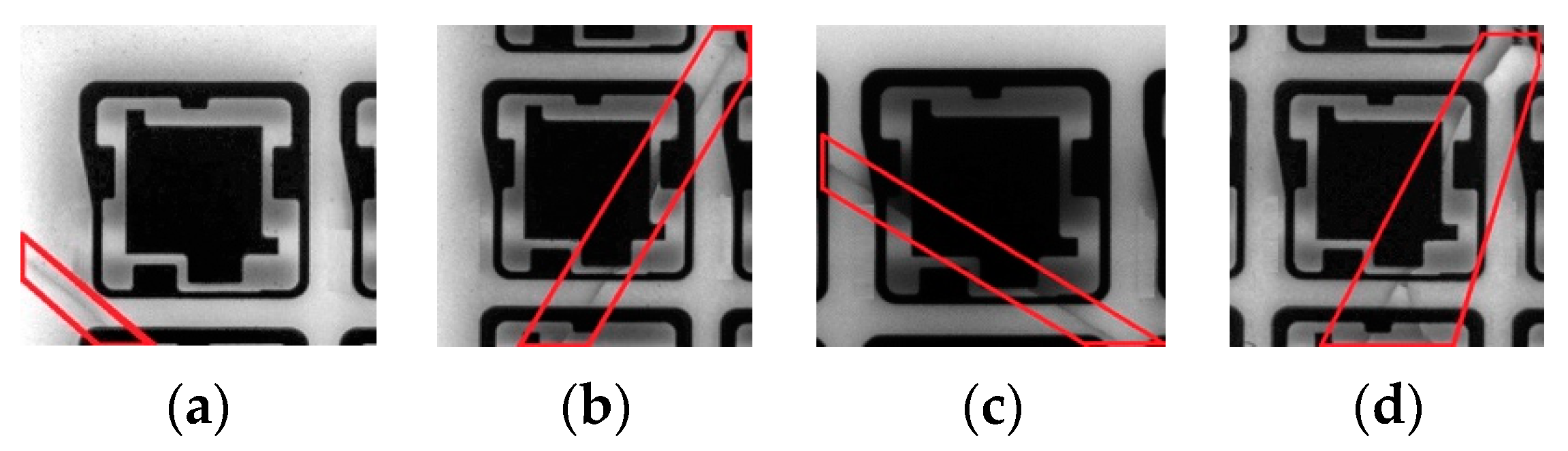
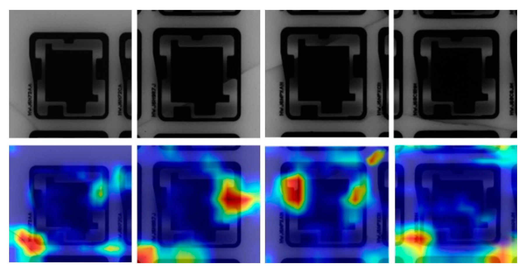
All samples were converted to grayscale by using AOI. The chipsets were mainly divided into three types on the basis of the defect distributions on the ceramic substrates (Figure 1). In Figure 1a, the defect is on the corner of the chipset. Figure 1b,c shows defects detected on the border of a chipset, and Figure 1d presents a defect found in the middle of a chipset. The cracks shown in Figure 1 can form into darkish flaws over the chipsets during production. For example, the defect displayed in Figure 1d is surrounded by other chips, occupying a major portion of the instances in the dataset. By contrast, the cracks in the corner occupy a much smaller portion of the instances compared with the center one. The degree of the imbalance problem varies when the data are not dispersed evenly. It can also arise from other features such as overlapping between classes or aggregate complicated information within the same domains of the class. For example, consider the chipset shown in Figure 1. The chip is placed in a grid array on a board and is inspected by using AOI before cutting it. The types of images differ on the basis of the position of the defect, brightness, and crack shape. The combination of these factors causes the imbalance problem to be complex. The distribution can vary depending on the brightness of the snapshots taken during AOI. For example, Figure 1a is brighter than Figure 1b–d. The cracks can be found in any shape or at any location. Some cracks may form unusual shapes as shown in Figure 1c,d, but most cracks form single lines, and that is illustrated with red bounded region in Figure 1. Because of the combination of these factors, no single standard can appropriately cluster images into groups in terms of the position, brightness, or crack shape. Some of the defect chipsets are shown in Figure 2 along with heat maps that illustrate where the defect regions are located. Therefore, our framework employed an unsupervised algorithm to cluster cracks into appropriate groups.
The uncertain locations and unpredictable darkness caused by cracks with a skewed distribution on a chipset surface cause the problem of imbalanced information. We address the imbalanced dataset problem by using deep models. In particular, we focus on data manipulation. The proposed method employed the K-means algorithm which is a pivot for balancing datasets. Features were acquired by feeding a balanced dataset to a CNN.
3.2. Unsupervised Balanced Sampling
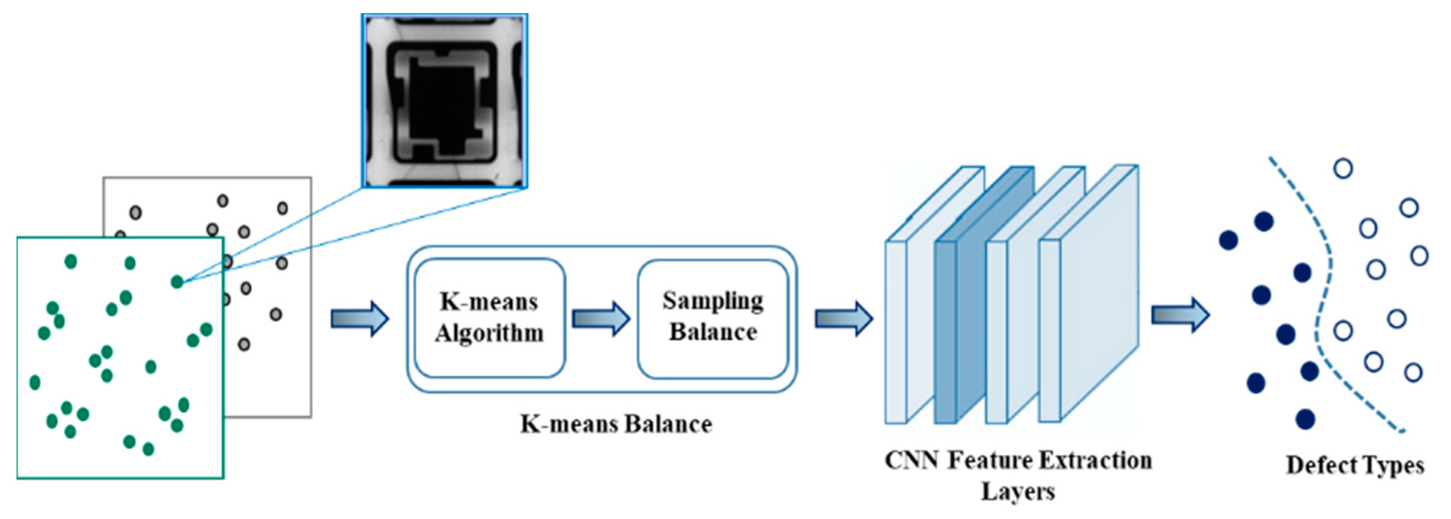
In our method, K-means balance, the K-means algorithm, and balanced sampling are merged into the training process to resolve the imbalance problem without the requirement of changing the skewed distribution of a raw dataset in advance. When an imbalanced dataset is obtained, in general, the proposed method oversamples the minority class or downsamples the majority class before splitting the dataset into training and validation datasets and then feeds the data to CNNs. However, the data manipulation methods may result in overgeneralization or information loss. Therefore, we propose an unsupervised method to alleviate both potential problems. To avoid the issues that might arise while handling a disproportionate dataset, the K-means balance method improves the training process by adapting to the frequency of data instances through controlling the speed of data increases and decreases. There are two main processes in the K-means balance method, as shown in Figure 3. First, the skewed inputs, defects, and nondefects are inputted through the K-means algorithm to perform unsupervised clustering. The proposed method divides the dataset into separate groups and computes the size of each cluster and mean m of all clusters as the number of balanced targets. Second, the difference between the size of each cluster and mean m to balance at given epoch is computed. Finally, a balanced sampling method randomly selects samples from each cluster for oversampling and subsampling along training epochs, which causes the model to be balanced.
We also found that although data were balanced, the learning of deep models fluctuated, or data overfitting occurred easily, if the dataset was too small. To overcome this problem, we added an extra hyper-parameter to adjust the average number of data for each cluster, and we set the value to 1.3 with grid search {1.0, 1.1, 1.2, 1.3, 1.4, 1.5}. The computed numbers of samples that were either oversampled or subsampled is associated with a hyperparameter that is used to control the speed of sample increases and decreases. We used grid search to find optimal values, namely 0.035 and 0.010, from {0.030, 0.035, 0.040} and {0.010, 0.015, 0.020}, respectively. The average number of data for each cluster was eventually reached by the end of the indicated epochs; we set 500 epochs on the basis of grid search {300, 400, 500}. Therefore, important information can be captured even though majority instances are subsampled, the features of minority instances can be obtained appropriately, and the overfitting issue can be avoided by changing the frequency of data occurrence. Samples are split into small batches prior to input to the CNN models during training. After the CNN models are trained, we perform classification on the test set.
3.3. Network Architecture
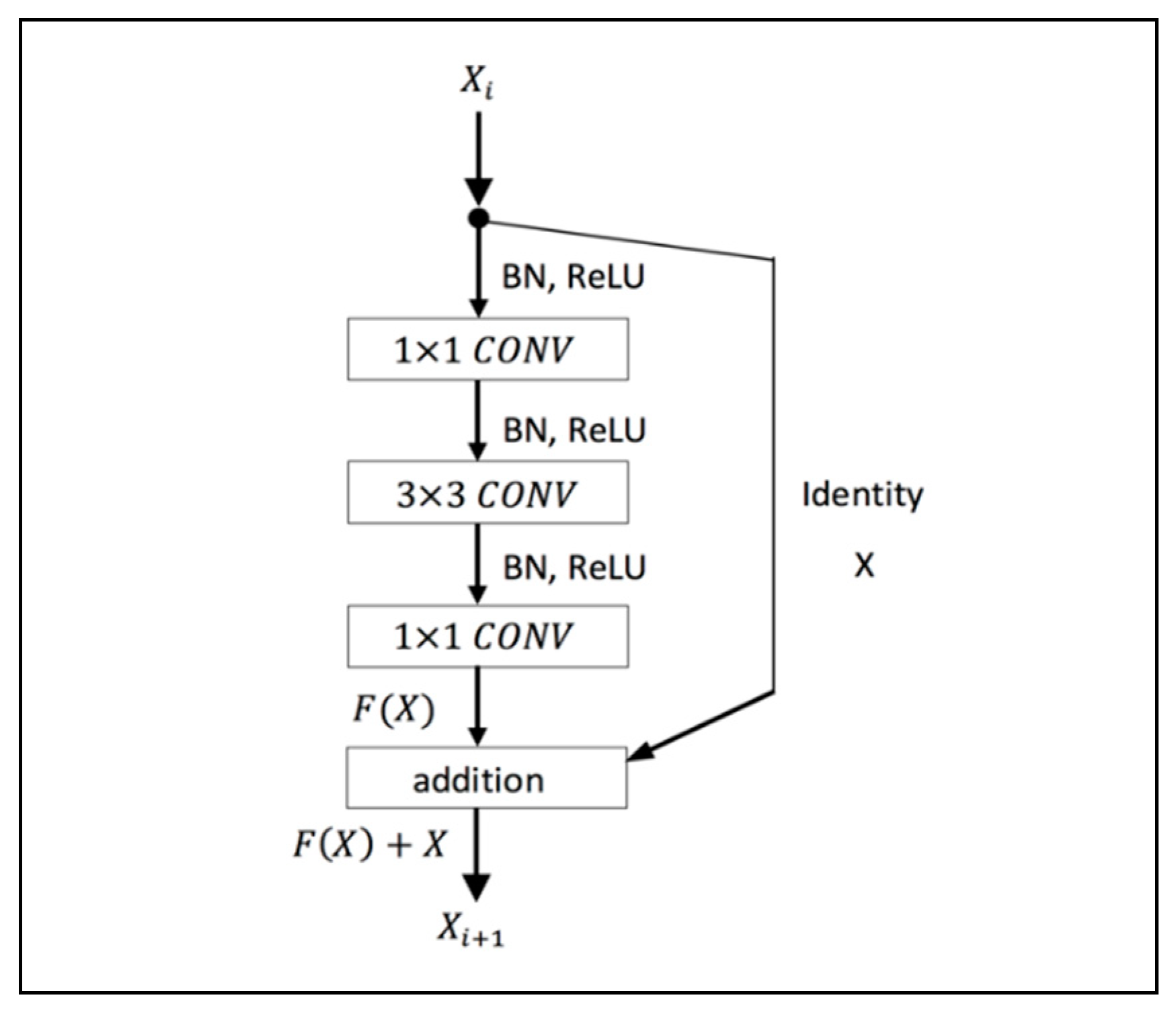
In deep learning network, the accuracy and efficiency of the model become saturated as the network depth increases. To solve the problem of degradation with an increase in the depth of the network, a residual framework is utilized (Figure 4).
This study employed a 29-layers ResNet composed of multiple residual building blocks, and each residual block includes multiple convolutional layers with a set of learnable filters and activation function. The residual block of the proposed architecture consists of a 1 × 1 convolutional layer to reduce dimension, a 3 × 3 convolutional layer, and a 1 × 1 convolutional layer to restore dimension. Down-sampling is performed by conv3_1 and conv4_1 with a stride of 2. The system’s structure is illustrated in Table 1. We directly use identity shortcuts when the input and output have the same dimensions. When the dimensions of the output are increased, the shortcut performs identity mapping with an extra zero-padding entry to increase dimensions. To avoid overfitting and increase model performance, preactivation batch normalization/ReLU nonlinearity is applied (Figure 4).
Network Implementation: Our implementation was slightly modified from a previously described implementation [29] to meet the hardware requirements. Table 1 lists the size of each layer used in defect detection. We resized the images to 200 × 200, instead of 224 × 224 as in [29]. The images were originally resized and randomly sampled from [246, 480] to ensure scale augmentation. However, as the defects in some cases occur around the borders of images, vital information might be lost if the resized images are randomly sampled, as was the case in [29]. We also conducted batch normalization immediately after each convolution and before activation. We trained all plain/residual nets from scratch. We employed an Adam optimizer with a small batch size of 24 because of the limited memory; the initial learning rate was 10−3. We did not conduct dropout as in [34], and performance was measured on the same test set within 5000 steps.
To account for the formation of varying crack shapes in any direction and to adapt to the inconsistency in the brightness of optical cameras, a sequence of operations was applied to each training image to make the models more robust.
- Left–right reflection: Randomly flip an image horizontally (left to right).
- Up–down reflection: Randomly flip an image vertically (upside down).
- Counterclockwise image rotation: Randomly rotate an image counterclockwise by 0°, 90°, 180°, or 270°.
- Slight image rotation: Randomly rotate an image by an angle between −10° and 10°.
- Brightness and darkness adjustment: Adjust the brightness or darkness of an image with a value randomly sampled by using a uniform distribution.
- Gaussian noise addition: Add Gaussian noise to an image with a value randomly sampled by using a uniform distribution.
- Gaussian blur addition: Blur out an image with a value randomly sampled by using a uniform distribution.
3.4. Balance Procedure
The procedure of the proposed approach is described as follows.
- Given a set of samples of class c, we apply the K-means algorithm by initializing stochastic cluster centroids for each class. Then, samples for each class are clustered into K groups.
- Compute the mean m of the number of data in all classes. The new average number of balanced target is then computed by the multiplication , where r denotes a scalar.
- The difference value between a subclass of c, and the mean is calculated by (C is the number of classes, = 2, defect and nondefect)
- The number of samples in subclass of c, , that are either oversampled or subsampled at a particular training epoch s, s = 1, 2, …, S, is calculated as follows .
- For each subclass of c, samples are randomly oversampled or subsampled along with the training epoch s.X is divided into small batches, and the batches are fed into CNNs.
- The procedure is repeated from step 4 to 6 in the next epoch until the entire procedure reaches the target balanced number.
The K-means balance algorithm is shown in Algorithm 1.
| Algorithm 1: K-means balance. |
| 1: , Initial stochastic centroids , hyper-parameter as a ratio used to adapt the average number of samples. 2: the updated set , and feed forward to CNN. 3: Apply K-means algorithm with random 4: Shuffle the positions of samples . 5: Compute the difference of each cluster. 6: Compute the number of samples to be oversampled or subsampled. 7: Oversample or subsample d samples drawn from the input x. 8: 9: 10: 12: 13: 13: 14: 18: 19: SHUFFLE () 20: |
4. Experimental Settings
We conducted an empirical study to evaluate the proposed method in two experimental settings. First, we compared the convergence speed and the accuracy of the models trained with various split distributions of the dataset. Second, we evaluated the precision of models with various levels of balancing parameters (balancing settings).
4.1. Datasets
The experiments were conducted using the state-of-the-art CNN ResNet [29], which has been recognized at many competitions such as ILSVRC and COCO 2015. Our dataset included 890 defect images and 3890 nondefect images, all of which were grayscale. From the dataset, 70% of the images were used for training, while the remaining 30% were used for validation. To compare the performance of imbalanced and balanced datasets, three training configurations were investigated, as shown in Table 2.
Imbalanced method: A raw dataset was directly split into training and validation datasets, and the model was trained with the imbalanced training dataset.
Subsampling method: Only the majority class of the raw dataset was subsampled, and the dataset was then split into training and validation datasets. Considering the small size of the datasets in this method, we increased the number of epochs to 1200 to match the number of training steps to those of the other two methods. In this method, we applied subsampling only to the training dataset to train the model.
Balancing method: The split setting in this method was the same as that of the imbalanced method; however, the proposed balancing method was applied during the training process. For defect detection, we used four clusters in the K-means algorithm, which is optimal for clustering. We applied the K-means balance setting to model the training process by using the imbalanced training dataset.
To compare performance, test data that were excluded from training and validation sets were evaluated. Experiments were run on a workstation with 12 Intel Xeon CPUs, 32 GB memory, and two GeForce GTX 1080 Ti graphics processing units on a TensorFlow platform. The classifiers were trained and validated through 10-fold cross-validation.
4.2. Evaluation Metrics
The performance of the proposed method was evaluated using four standard metrics such as accuracy, precision, recall, and F1 score. Accuracy is defined as the ratio of accurately predicted observations to total observations. Precision is the proportion of correctly predicted positive observations to all positive observations in the class, whereas recall is the proportion of correctly predicted positive observations to all positive observations in the actual class. Finally, F1 score represents weighted average of precision and recall that accounts for both false positives and false negatives. They are defined mathematically as
where TP indicates the true positive, TN is the true negative, FP is the false positive, and FN is the false negative. In an ideal model, the precision and recall rates are equal to 1. The F1 score is a quantitative metric that represents the balance between precision and recall.
5. Discussion
Tenfold cross-validation was performed to compare the performance of the three training settings—imbalanced, subsampling, and balancing methods. All the trained models were evaluated using the same testing dataset. In the subsampling method, the model was trained using 1200 epochs. Moreover, in the imbalanced and balancing methods, the models were trained with 500 epochs. To compare the subsampling method with the remaining settings, we plotted the figures by displaying the training steps instead of the epochs.
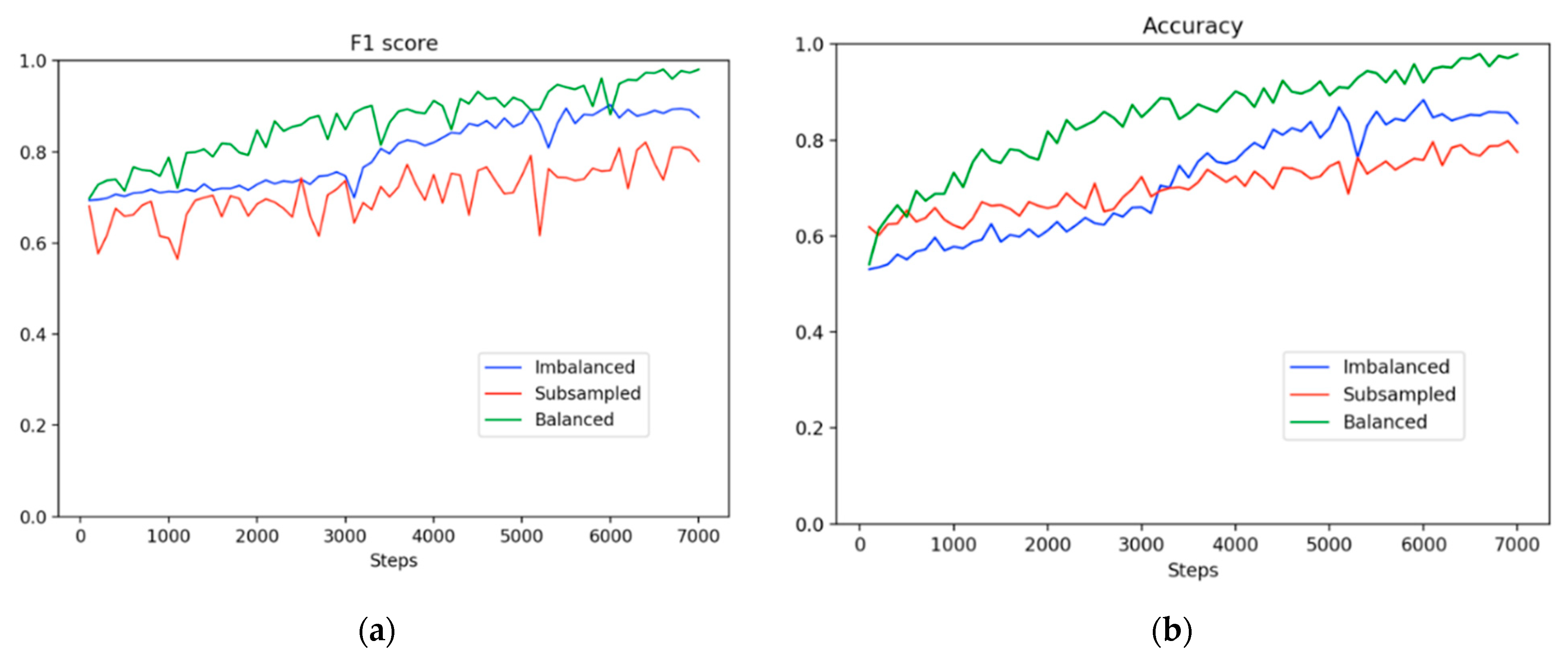
Figure 5 shows the learning trajectories in F1 scores and accuracy. The learning trajectories represent the predicted scores on the same test set for three experimental settings along 7000 training steps. The trajectories indicate that the F1 scores improved moderately before 3000 steps in the imbalanced method. For the subsampling method, there was a downward fluctuation in the F1 score and a leveling-off trend during the entire training process even though the dataset was balanced. The subsampling method had a higher probability of overfitting due to the extremely small dataset used. By contrast, at the beginning of the training period, the balancing method demonstrated a superior precision value of 5% or higher compared with the imbalanced and subsampling methods. Subsequently, the precision value of the balancing method continued to increase; however, the value of the imbalanced method had a slight upward trend. Moreover, the small size of the dataset caused a downward trend in the precision value in the subsampling method from the start of the training. Overall, the balancing method not only achieved a higher accuracy than the imbalanced method, as shown in Figure 5, but it also attained a superior concentration at high scores, as shown in Figure 6. Moreover, our proposed method outperformed the imbalanced and subsampling methods from the beginning of the training process, although the split setting of our method was the same as that in the imbalanced method.
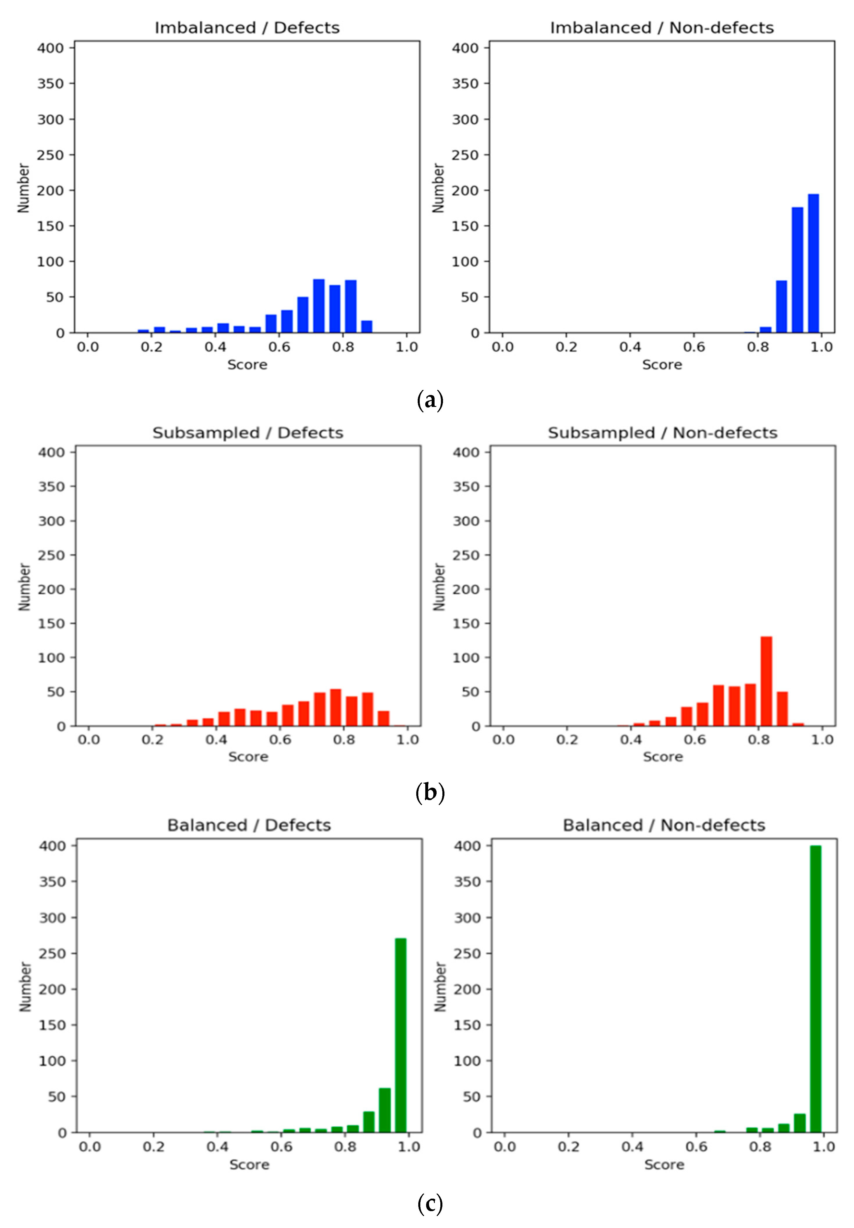
Figure 6 shows histograms of the evaluation scores in each training setting. The histograms on the left side illustrate the scores of defect classification, whereas those on the right side show those of nondefect classification. In general, the scores in the balanced method were equal to or higher than 0.85 and greater than those of the imbalanced and subsampling methods for the defect and nondefect image groups. Clearly, the nondefect image group had higher confidence scores than the defect group. A common aspect between the imbalanced and subsampling methods was that the sizes of the training datasets for the defects were the same. However, the nondefect samples in the subsampling method were reduced to the same size as the defect samples. The scores in the subsampling method were spread out due to the leveling off, as shown in Figure 5. This implies that the results obtained through downsampling were poorer than those obtained using the imbalanced method because of the discarding of information. Moreover, the small dataset deteriorated model learning and resulted in overgeneralization. By contrast, in the imbalanced method, the scores for defect identification were widespread, whereas those for nondefect identification were concentrated at high values. This raised a question regarding how nondefects affect defects during model learning; an experiment was conducted to answer this question. For both defects and nondefects, the balanced method had superior confidence scores, and the frequency of the scores was concentrated at higher values.
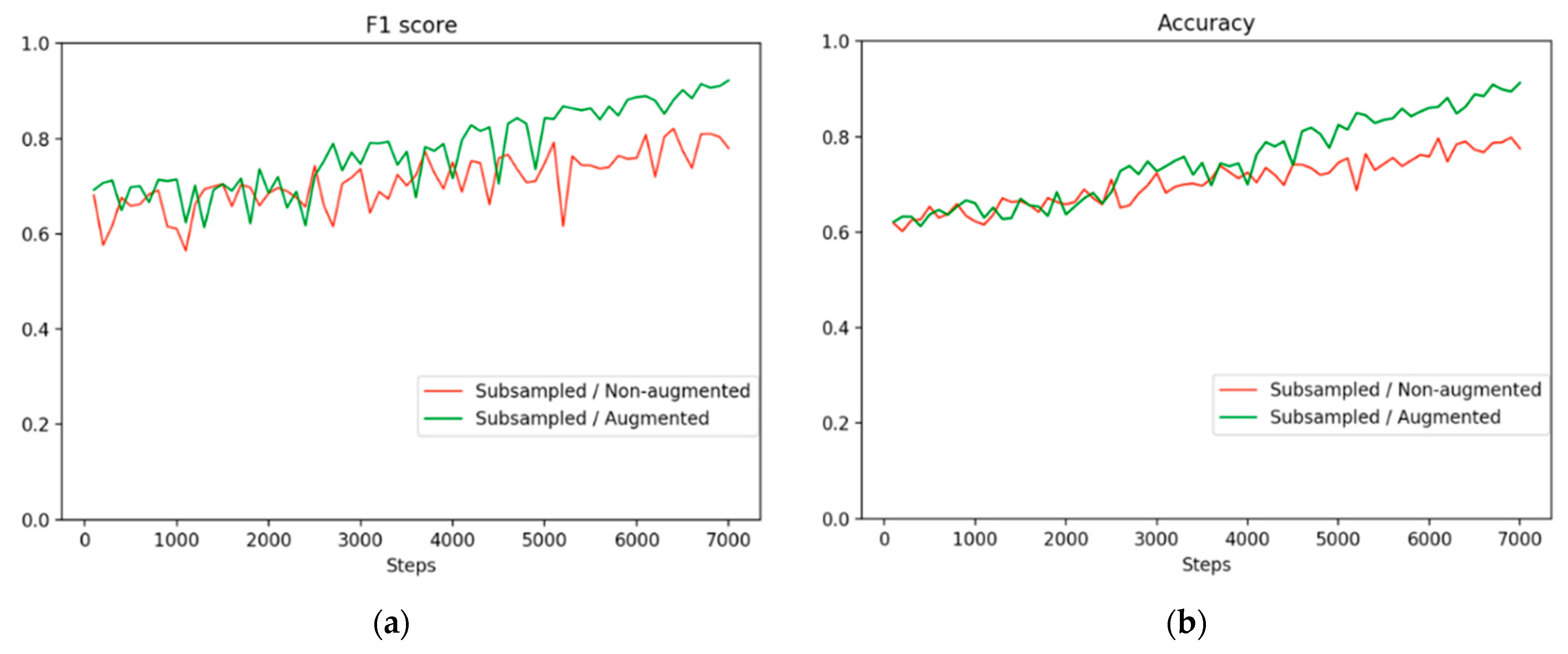
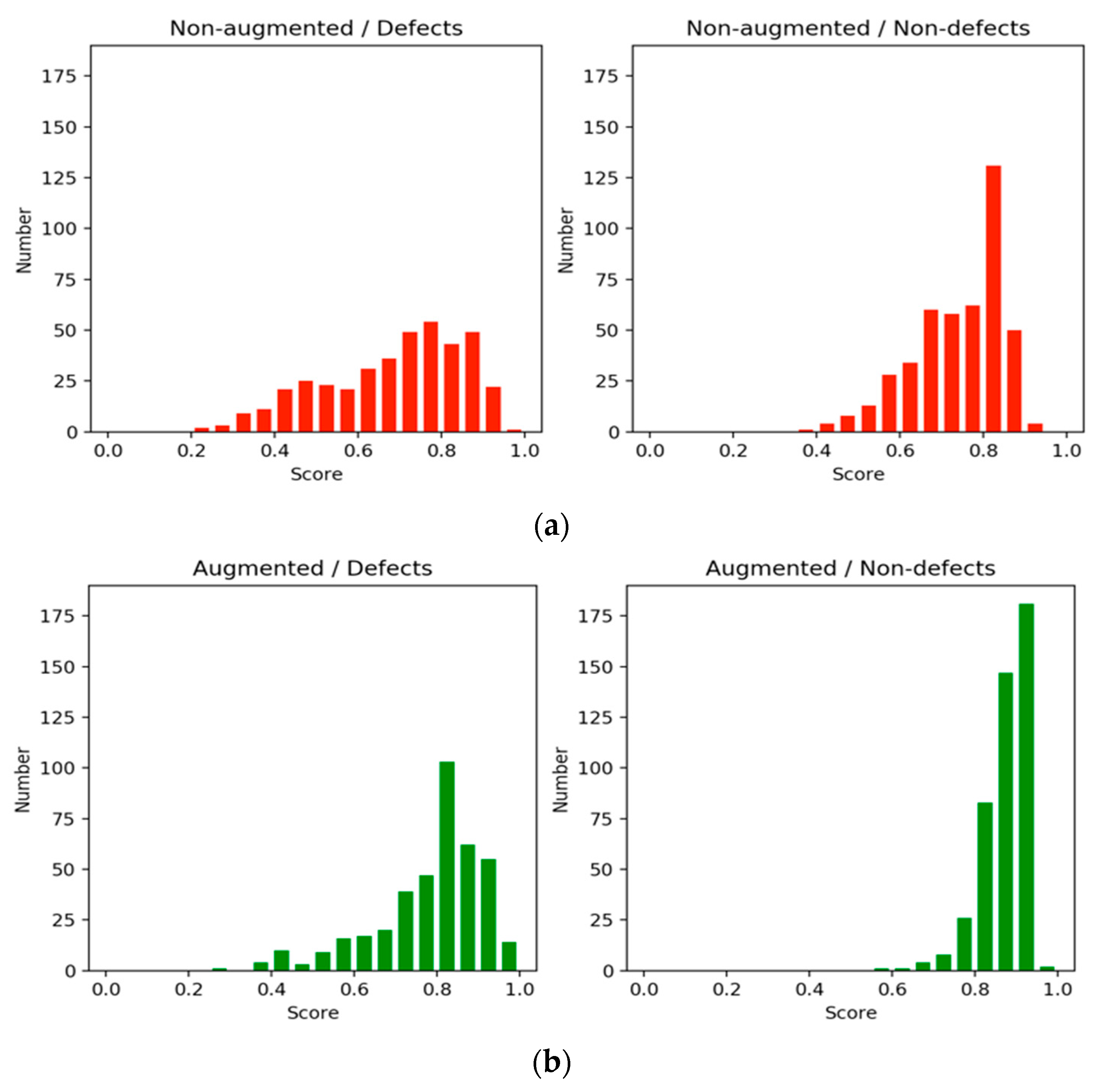
On the basis of how defects and nondefects influence each other, we conducted an additional experiment on subsampling with 10-fold cross-validation. The method used in this experiment was called an augmented method, and its results were compared with those of the original, or nonaugmented, method. The number of nondefects increased by a factor of 1.25 compared with that of defects. Figure 7a shows the F1 scores for the nonaugmented method and augmented method learning trajectories. Figure 7b displays the accuracy trajectories. Figure 8a displays a comparison of the score distribution for defects and nondefects in 7000 steps of the nonaugmented method. Figure 8b displays a comparison of the score distribution of the augmented method. The augmented method exhibited a stable upward trend compared with the nonaugmented method, although its distribution was slightly skewed. The distribution of scores demonstrates that both defects and nondefects tended to be higher and to be more concentrated at higher values. Our observations indicated that a large amount of information from nondefects, which might be crucial for identifying defects, was ignored, potentially causing the model to learn fewer features. Thus, the frequency of nondefect sampling has an effect on the results for defects.
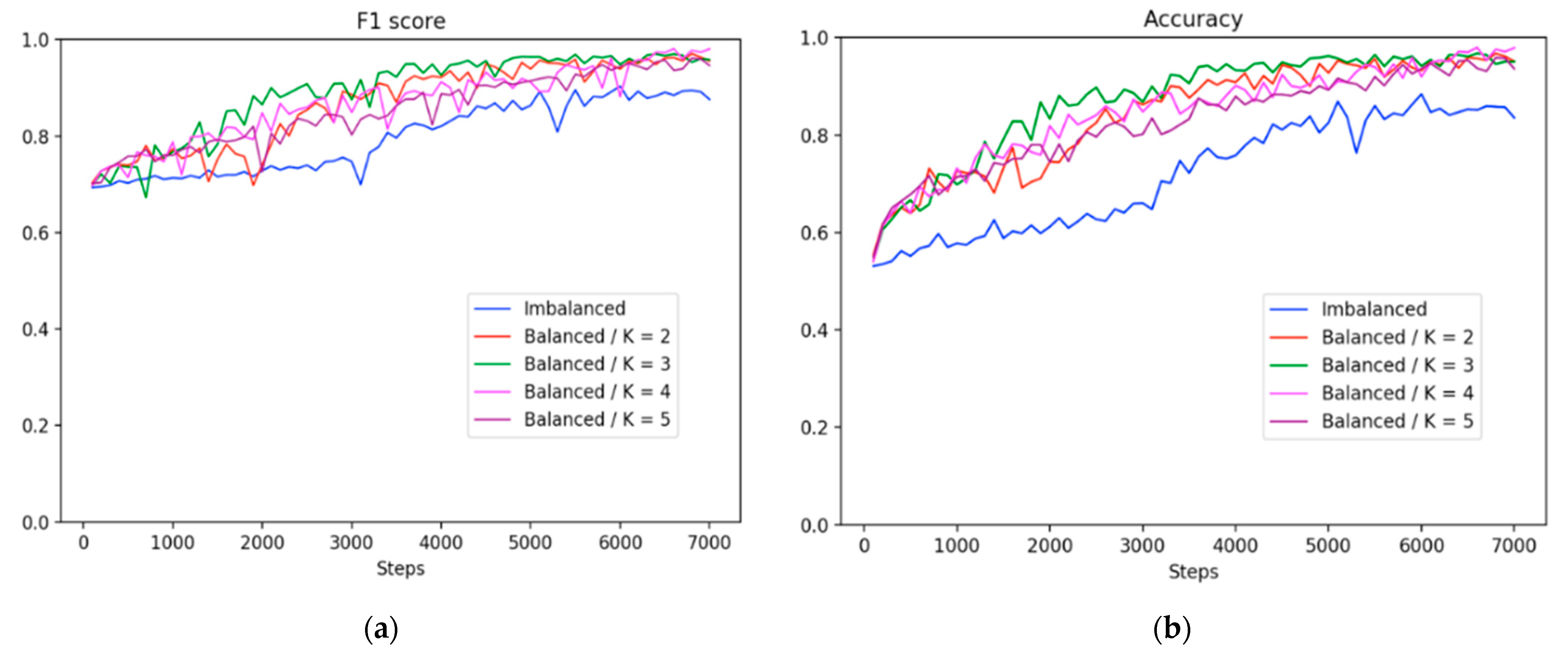
Furthermore, we also conducted an experiment by using two to five clusters to determine the various performance of the clusters, as shown in Figure 9 and Figure 10. Overall, the balancing method outperformed the imbalanced strategy across all clusters. For instance, the learning trajectories in Figure 9 revealed that K = 4 outperformed the other clusters in terms of F1 score and accuracy matrices.
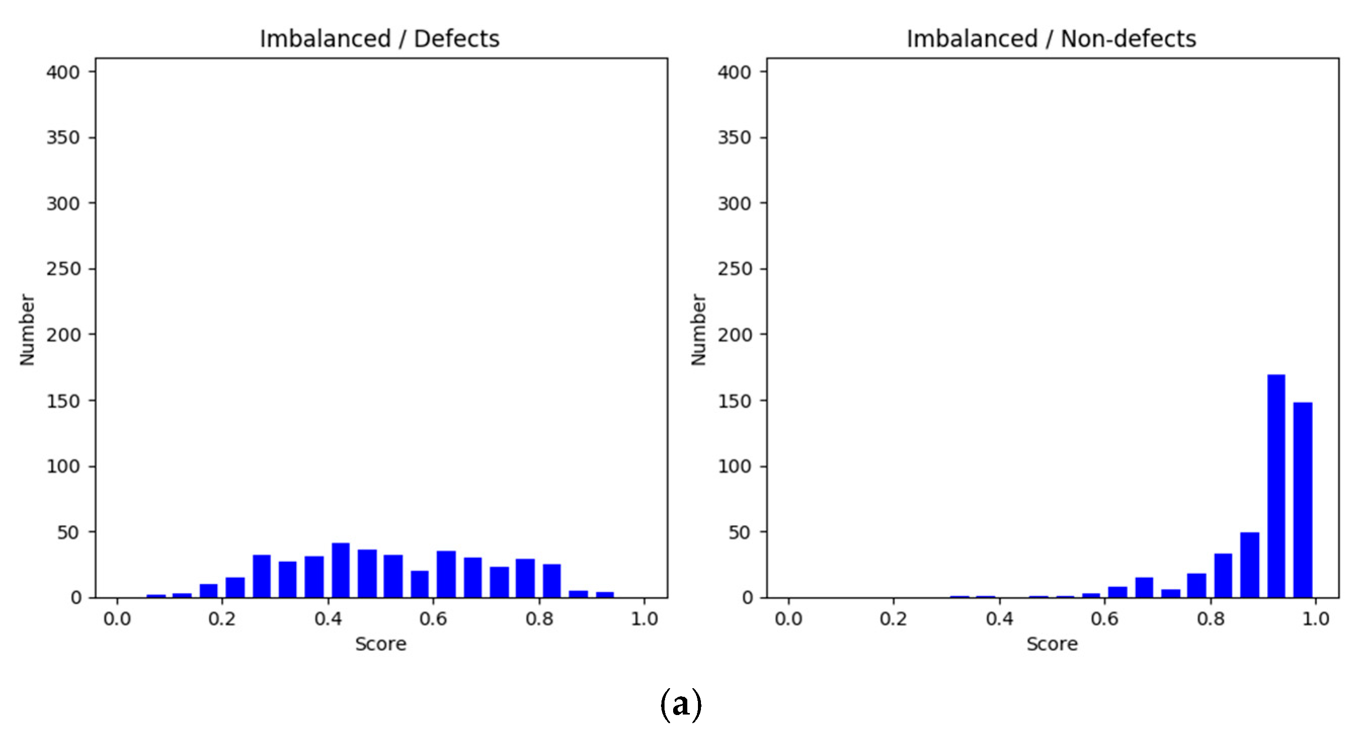
Additionally, histogram in Figure 10 compares the confidence level of the two methods. The X-axis represents the confidence interval range between 0.0 and 1.0, and the Y-axis is the confidence values of the sample size. In the imbalanced approach, the number of nondefects was higher than the number of defects, making the degree of confidence in nondefects more concentrated, but it was not effective and highly confident to distinguish the categories on the defect samples (Figure 10a). In the balanced method, the confidence score of the defect category was more concentrated with higher scores (Figure 10b–e). However, among them all, K = 4 (Figure 10d) showed an improved confidence score, and the number of nondefects was above 350. Therefore, we employed four clusters in most experiments for comparisons with other clusters.
Table 3 shows the final accuracy and F1 score of each setting when the iterations cease at 7000. This clearly demonstrates the effectiveness of integrating unsupervised balancing with the CNN in our framework.
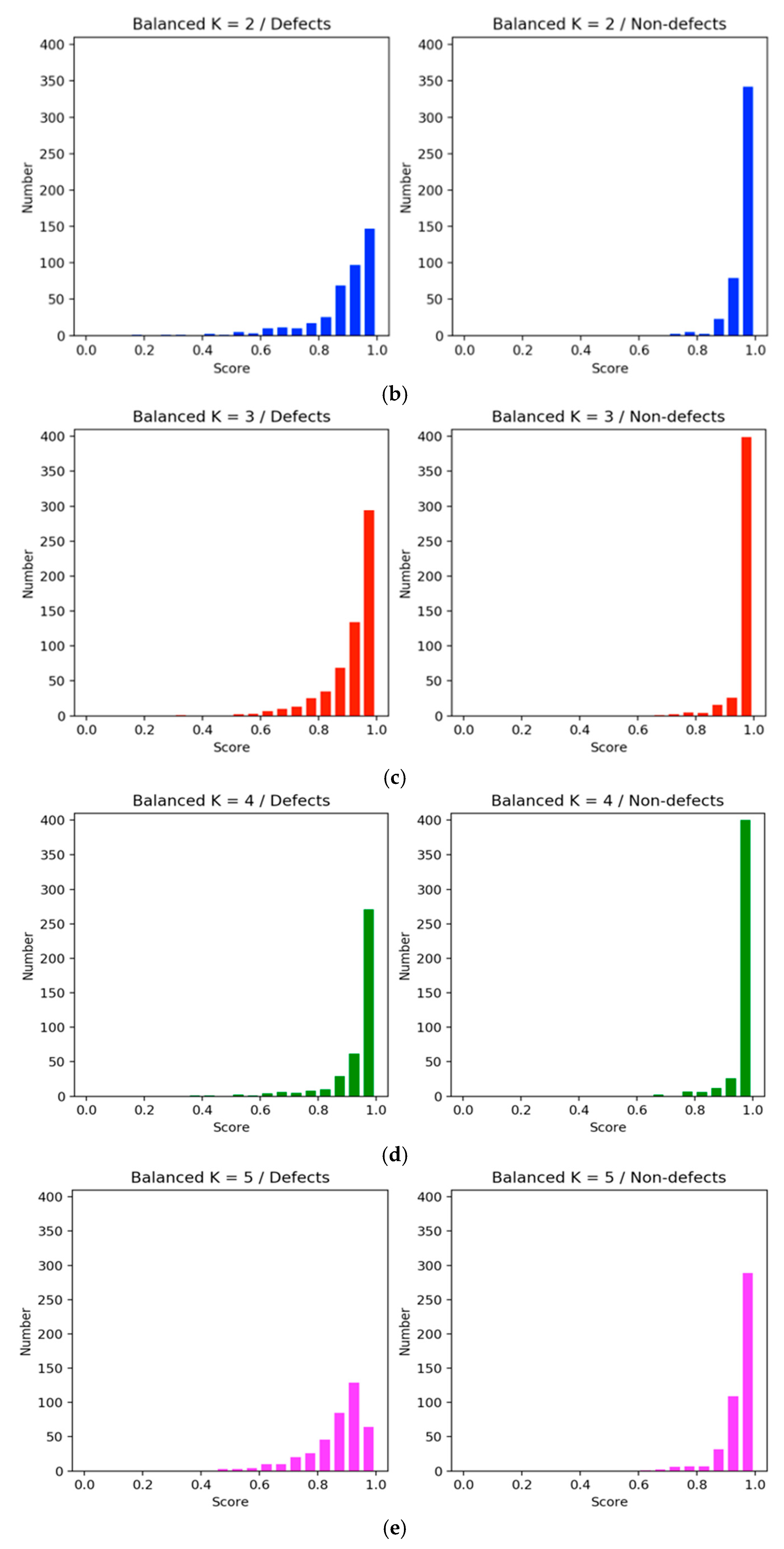
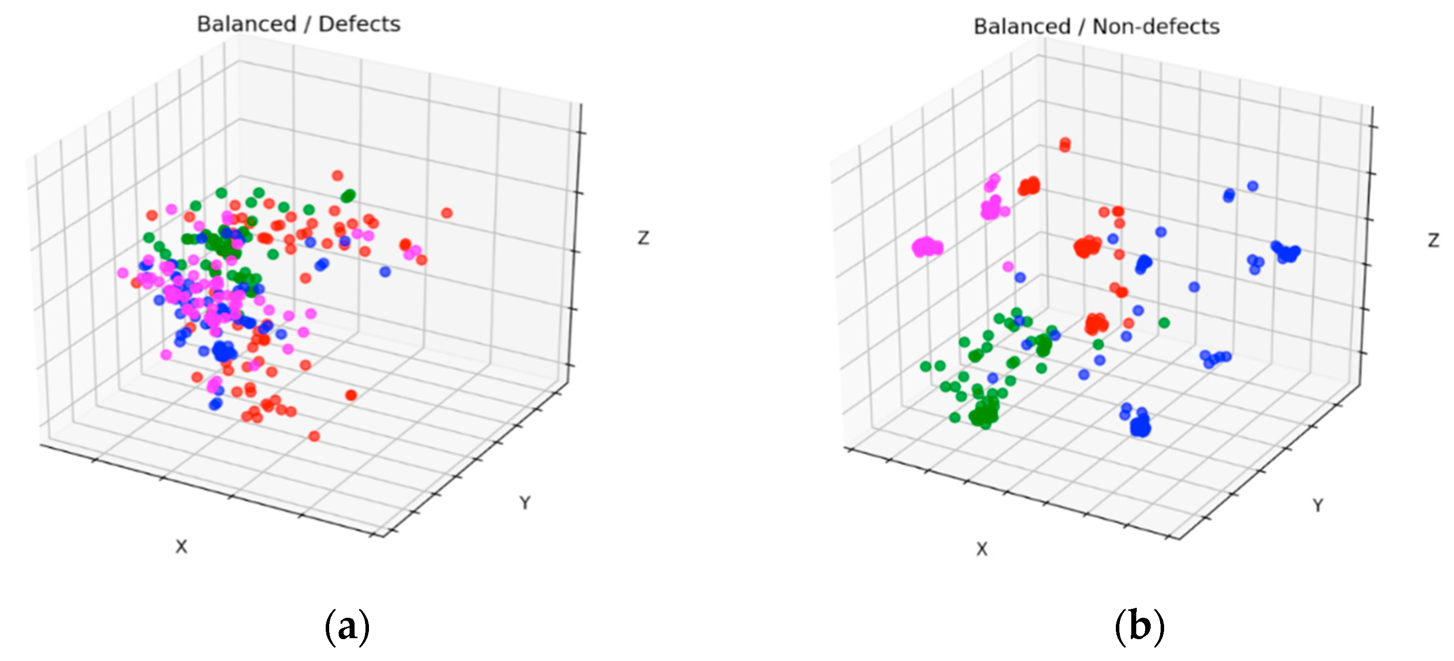
Figure 11 and Figure 12 show scatter results of the datasets with four clusters before and after balancing for defects and nondefects, respectively. These figures were plotted by applying PCA [35] to one of the 10-fold experimental results. By comparing Figure 11a with Figure 12a, we observed that the new stochastic points in Figure 12a represent the balanced minority examples, which become widespread when the minority instances are augmented with a sequence of filters to virtually enlarge training set size and avoid overfitting. In contrast to the SMOTE method, which creates new duplicated examples by interpolating the neighboring minority class, our proposed method will not extend dissimilar images because it has a tendency toward overgeneralization. In Figure 11b, small disjunctions appear, although nondefects account for the majority of the dataset. In other words, a small portion of minority examples that should be oversampled exists. In particular, the green dots in Figure 12b show the oversampled minority examples in nondefects.
6. Conclusions
In this study, we observed that the learning process oscillates and tends toward overfitting during training of the CNNs when a small dataset was used, even if it was balanced. The reason for the imbalanced classes and the similarity of surfaces must be identified. Therefore, we presented a method to balance the complexity both between classes and within classes, which reduced FPs in defect classification among chip images by changing the occurrence frequency of the minority and majority instances along the training epochs. We demonstrated that the proposed method achieved superior performance in comparison with imbalanced and oversampling learning methods. The empirical results demonstrated the effectiveness of our method in classifying defects with highly skewed classes and highly uneven instance distributions.
Since there were limited real crack datasets available, it is better to collect more crack datasets from different manufacturing procedures or from different data sources to further verify the transfer learning method and the applicability of the proposed method in the future.
Author Contributions
Conceptualization, Y.-P.H. and C.-M.S.; methodology, Y.-P.H. and C.-M.S.; software, C.-M.S. and H.B.; validation, Y.-P.H., C.-M.S. and Y.-L.T.; formal analysis, Y.-P.H. and C.-M.S.; investigation, Y.-P.H., C.-M.S., H.B. and Y.-L.T.; resources, Y.-P.H. and Y.-L.T.; data curation, Y.-P.H. and Y.-L.T.; writing—original draft preparation, Y.-P.H. and C.-M.S.; writing—review and editing, Y.-P.H., C.-M.S. and H.B.; visualization, Y.-P.H. and Y.-L.T.; supervision, Y.-P.H. and Y.-L.T.; project administration, Y.-P.H.; funding acquisition, Y.-P.H. and Y.-L.T.; All authors have read and agreed to the published version of the manuscript.
Funding
This work was supported in part by the Ministry of Science and Technology, Taiwan, under grant numbers MOST106-2221-E-027-001 and MOST108-2221-E-027-111-MY3, and in part by the National Taipei University of Technology International Joint Research Project, under Grants NTUT-IJRP-109-03 and NTUT-IJRP-110-01.
Conflicts of Interest
The authors declare no conflict of interest.
References
- Yang, J.; Li, S.; Wang, Z.; Dong, H.; Wang, J.; Tang, S. Using Deep Learning to Detect Defects in Manufacturing: A Comprehensive Survey and Current Challenges. Materials 2020, 13, 5755. [Google Scholar] [CrossRef] [PubMed]
- Park, Y.-J.; Fan, S.-K.S.; Hsu, C.-Y. A Review on Fault Detection and Process Diagnostics in Industrial Processes. Processes 2020, 8, 1123. [Google Scholar] [CrossRef]
- Czimmermann, T.; Ciuti, G.; Milazzo, M.; Chiurazzi, M.; Roccella, S.; Oddo, C.M.; Dario, P. Visual-Based Defect Detection and Classification Approaches for Industrial Applications—A Survey. Sensors 2020, 20, 1459. [Google Scholar] [CrossRef] [PubMed] [Green Version]
- Sheu, R.-K.; Chen, L.-C.; Pardeshi, M.S.; Pai, K.-C.; Chen, C.-Y. AI Landing for Sheet Metal-Based Drawer Box Defect Detection Using Deep Learning (ALDB-DL). Processes 2021, 9, 768. [Google Scholar] [CrossRef]
- Paraskevoudis, K.; Karayannis, P.; Koumoulos, E.P. Real-Time 3D Printing Remote Defect Detection (Stringing) with Computer Vision and Artificial Intelligence. Processes 2020, 8, 1464. [Google Scholar] [CrossRef]
- Ferguson, M.K.; Ronay, A.; Lee, Y.T.; Law, K.H. Detection and Segmentation of Manufacturing Defects with Convolutional Neural Networks and Transfer Learning. Smart Sustain. Manuf. Syst. 2018, 2, 1–43. [Google Scholar] [CrossRef]
- Takada, Y.; Shiina, T.; Usami, H.; Iwahori, Y.; Bhuyan, M.K. Defect Detection and Classification of Electronic Circuit Boards Using Keypoint Extraction and CNN Features. In Proceedings of the Ninth International Conference on Pervasive Patterns and Application, Athens, Greece, 19–23 February 2017. [Google Scholar]
- Pereira, S.; Pinto, A.; Alves, V.; Silva, C.A. Brain Tumor Segmentation Using Convolutional Neural Networks in MRI Images. IEEE Trans. Med. Imaging 2016, 35, 1240–1251. [Google Scholar] [CrossRef] [PubMed]
- Setio, A.A.A.; Ciompi, F.; Litjens, G.; Gerke, P.; Jacobs, C.; Van Riel, S.J.; Wille, M.M.W.; Naqibullah, M.; Sánchez, C.I.; van Ginneken, B. Pulmonary Nodule Detection in CT images: False Positive Reduction Using Multi-View Convolutional Networks. IEEE Trans. Med. Imaging 2016, 35, 1160–1169. [Google Scholar]
- Sakamoto, M.; Nakano, H.; Zhao, K.; Sekiyama, T. Multi-Stage Neural Networks with Single-Sided Classifiers for False Positive Reduction and Its Evaluation Using Lung X-Ray CT Images. In Proceedings of the 19th International Conference on Image Analysis and Processing, Catania, Italy, 11–15 September 2017. [Google Scholar]
- Yan, Y.; Chen, M.; Shyu, M.-L.; Chen, S.-C. Deep Learning for Imbalanced Multimedia Data Classification. In Proceedings of the IEEE International Symposium on Multimedia, Miami, FL, USA, 14–16 December 2015. [Google Scholar]
- Arthur, D.; Vassilvitskii, S. k-means++: The Advantages of Careful Seeding. In Proceedings of the Eighteenth Annual ACM-SIAM Symposium on Discrete Algorithms, New Orleans, LA, USA, 7–9 January 2007. [Google Scholar]
- Sculley, D. Web-scale K-means Clustering. In Proceedings of the 19th International Conference on World Wide Web, Raleigh, NC, USA, 26–30 April 2010; pp. 1177–1178. [Google Scholar]
- He, H.; Garcia, E.A. Learning from Imbalanced Data. IEEE Trans. Knowl. Data Eng. 2009, 21, 1263–1284. [Google Scholar]
- Liu, M.; Miao, L.; Zhang, D. Two-stage Cost-sensitive Learning for Software Defect Prediction. IEEE Trans. Reliab. 2014, 63, 676–686. [Google Scholar] [CrossRef]
- Lu, J.; Liong, V.E.; Zhou, J. Cost-Sensitive local binary feature learning for facial age estimation. IEEE Trans. Image Process. 2015, 24, 5356–5368. [Google Scholar] [CrossRef]
- Wang, S.; Liu, W.; Wu, J.; Cao, L.; Meng, Q.; Kennedy, P.J. Training deep neural networks on imbalanced data sets. In Proceedings of the IEEE International Joint Conference on Neural Networks, Vancouver, BC, Canada, 24–29 July 2016. [Google Scholar]
- Maciejewski, T.; Stefanowski, J. Local Neighborhood Extension of SMOTE for Mining Imbalanced Data. In Proceedings of the IEEE Symposium on Computational Intelligence and Data Mining, Paris, France, 11–15 April 2011. [Google Scholar]
- Chawla, N.V.; Bowyer, K.W.; Hall, L.O.; Kegelmeyer, W.P. Smote: Synthetic Minority Over-sampling Technique. J. Artif. Intell. Res. 2002, 16, 321–357. [Google Scholar] [CrossRef]
- Dablain, D.; Krawczyk, B.; Chawla, N.V. DeepSMOTE: Fusing Deep Learning and SMOTE for Imbalanced Data. arXiv 2021, arXiv:2105.02340. [Google Scholar]
- Blagus, R.; Lusa, L. SMOTE for High-dimensional Class-Imbalanced Data. BMC Bioinform. 2013, 14, 1–19. [Google Scholar] [CrossRef] [PubMed] [Green Version]
- Johnson, J.M.; Khoshgoftaar, T.M. Survey on Deep Learning with Class Imbalance. J. Big Data 2014, 6, 1–54. [Google Scholar] [CrossRef]
- Khan, S.H.; Hayat, M.; Bennamoun, M.; Sohel, F.; Togneri, R. Cost Sensitive Learning of Deep Feature Representations from Imbalanced Data. IEEE Trans. Neural Netw. Learn. Syst. 2017, 29, 3573–3587. [Google Scholar] [PubMed] [Green Version]
- Simonyan, K.; Zisserman, A. Very Deep Convolutional Networks for Large-scale Image Recognition. arXiv 2014, arXiv:1409.1556. [Google Scholar]
- Szegedy, C.; Liu, W.; Jia, Y.; Sermanet, P.; Reed, S.; Anguelov, D.; Erhan, D.; Vanhoucke, V.; Rabinovich, A. Going Deeper with Convolutions. arXiv 2014, arXiv:1409.4842. [Google Scholar]
- He, K.; Zhang, X.; Ren, S.; Sun, J. Identity Mappings in Deep Residual Networks. arXiv 2016, arXiv:1603.05027. [Google Scholar]
- Szegedy, C.; Vanhoucke, V.; Ioffe, S.; Shlens, J.; Wojna, Z. Rethinking the Inception Architecture for Computer Vision. arXiv 2014, arXiv:1512.00567. [Google Scholar]
- Szegedy, C.; Ioffe, S.; Vanhoucke, V.; Alemi, A.A. Inception-v4, Inception-ResNet and the Impact of Residual Connections on Learning. arXiv 2016, arXiv:1602.07261. [Google Scholar]
- He, K.; Zhang, X.; Ren, S.; Sun, J. Deep Residual Learning for Image Recognition. In Proceedings of the IEEE Conference on Computer Vision and Pattern Recognition, Las Vegas, NV, USA, 27–30 June 2016. [Google Scholar]
- Ando, S.; Huang, C.-Y. Deep Over-Sampling Framework for Classifying Imbalanced Data. In Proceedings of the European Conference on Machine Learning and Principles and Practice of Knowledge Discovery in Databases, Skopje, Macedonia, 18–22 September 2017. [Google Scholar]
- Huang, C.; Li, Y.; Change Loy, C.; Tang, X. Learning Deep Representation for Imbalanced Classification. In Proceedings of the IEEE Conference on Computer Vision and Pattern Recognition, Seattle, WA, USA, 27–30 June 2016; pp. 5375–5384. [Google Scholar]
- Yang, B.; Fu, X.; Sidiropoulos NDHong, M. Towards K-means-friendly Spaces: Simultaneous Deep Learning and Clustering. arXiv 2016, arXiv:1610.04794. [Google Scholar]
- Gong, Y.; Liu, L.; Ming, Y.; Bourdev, L. Compressing Deep Convolutional Networks Using Vector Quantization. arXiv 2014, arXiv:1412.6115. [Google Scholar]
- Castro, C.L.; Braga, A.P. Novel Cost-sensitive Approach to Improve the Multilayer Perceptron Performance on Imbalanced Data. IEEE Trans. Neural Netw. Learn. Syst. 2013, 24, 888–899. [Google Scholar] [CrossRef] [PubMed]
- Tipping, M.E.; Bishop, C.M. Mixtures of Probabilistic Principal Component Analyzers. Neural Comput. 1999, 11, 443–482. [Google Scholar] [CrossRef]
Figure 1.
Defects in chipset at various positions on a substrate. (a) In the corner, (b) and (c) on borders, and (d) in the middle.
Figure 1.
Defects in chipset at various positions on a substrate. (a) In the corner, (b) and (c) on borders, and (d) in the middle.

Figure 2.
Defect chipsets with associated heat maps where red color indicates the locations of defect parts.
Figure 2.
Defect chipsets with associated heat maps where red color indicates the locations of defect parts.

Figure 3.
Framework of the proposed method.

Figure 4.
Building block in residual learning.

Figure 5.
Comparison of the learning trajectories. (a) F1 score and (b) accuracy.

Figure 6.
Comparison of the histograms of the scores of various methods. (a) Imbalanced, (b) subsampled, and (c) balanced.
Figure 6.
Comparison of the histograms of the scores of various methods. (a) Imbalanced, (b) subsampled, and (c) balanced.

Figure 7.
Performance comparison between nonaugmented and augmented methods. (a) F1 score and (b) accuracy.
Figure 7.
Performance comparison between nonaugmented and augmented methods. (a) F1 score and (b) accuracy.

Figure 8.
Comparison of the score distribution. (a) Nonaugmented method and (b) augmented method.

Figure 9.
Comparison of the learning trajectories for various clusters. (a) F1 score and (b) accuracy.
Figure 9.
Comparison of the learning trajectories for various clusters. (a) F1 score and (b) accuracy.

Figure 10.
Performance comparisons of various numbers of clusters. (a) Imbalanced, (b) two clusters, (c) three clusters, (d) four clusters, and (e) five clusters.
Figure 10.
Performance comparisons of various numbers of clusters. (a) Imbalanced, (b) two clusters, (c) three clusters, (d) four clusters, and (e) five clusters.


Figure 11.
Scatter comparisons of the training data with four clusters for (a) defects and (b) non-defects in the imbalanced method.
Figure 11.
Scatter comparisons of the training data with four clusters for (a) defects and (b) non-defects in the imbalanced method.

Figure 12.
Scatter comparisons of the training dataset with four clusters for (a) defects and (b) nondefects in the balanced method.
Figure 12.
Scatter comparisons of the training dataset with four clusters for (a) defects and (b) nondefects in the balanced method.


Table 1.
Detailed architecture of 29-layers ResNet.
| Layer Name | Output Size | 29 Layers |
|---|---|---|
| input | 200 × 200 | read input image |
| conv1 | 200 × 200 | 3 × 3, 64, stride 1, ReLU |
| conv2_x | 200 × 200 | , |
| conv3_x | 100 × 100 | |
| conv4_x | 50 × 50 | |
| batch normalization, ReLU | ||
| output | 1 × 1 | average pool, 2-d fc, softmax |
Table 2.
Ceramic substrate defect and nondefect data distribution.
| Name | Method | Total Number | Defects | Non-Defects |
|---|---|---|---|---|
| Training set | Imbalanced | 334 | 62 | 272 |
| Subsampled | 124 | 62 | 62 | |
| Balanced | 334 | 62 | 272 | |
| Validation set | Imbalanced | 144 | 27 | 117 |
| Subsampled | 354 | 27 | 327 | |
| Balanced | 144 | 27 | 117 | |
| Test set | 853 | 400 | 453 |
Table 3.
Performance evaluation of ceramic substrate defect.
| Training Setting | Accuracy (%) | Precision | Recall | F1 Score (%) |
|---|---|---|---|---|
| Imbalanced | 82.5 | 87.3 | 85.6 | 86.4 |
| Subsampled | 77.5 | 77.0 | 78.7 | 78.0 |
| Balanced | 97.9 | 98.5 | 97.7 | 98.1 |
Publisher’s Note: MDPI stays neutral with regard to jurisdictional claims in published maps and institutional affiliations. |
© 2021 by the authors. Licensee MDPI, Basel, Switzerland. This article is an open access article distributed under the terms and conditions of the Creative Commons Attribution (CC BY) license (https://creativecommons.org/licenses/by/4.0/).
Share and Cite
MDPI and ACS Style
Huang, Y.-P.; Su, C.-M.; Basanta, H.; Tsai, Y.-L. Imbalance Modelling for Defect Detection in Ceramic Substrate by Using Convolutional Neural Network. Processes 2021, 9, 1678. https://0-doi-org.brum.beds.ac.uk/10.3390/pr9091678
AMA Style
Huang Y-P, Su C-M, Basanta H, Tsai Y-L. Imbalance Modelling for Defect Detection in Ceramic Substrate by Using Convolutional Neural Network. Processes. 2021; 9(9):1678. https://0-doi-org.brum.beds.ac.uk/10.3390/pr9091678
Chicago/Turabian StyleHuang, Yo-Ping, Chun-Ming Su, Haobijam Basanta, and Yau-Liang Tsai. 2021. "Imbalance Modelling for Defect Detection in Ceramic Substrate by Using Convolutional Neural Network" Processes 9, no. 9: 1678. https://0-doi-org.brum.beds.ac.uk/10.3390/pr9091678
Note that from the first issue of 2016, this journal uses article numbers instead of page numbers. See further details here.