Optimization of Cascade Cooling System Based on Lithium Bromide Refrigeration in the Polysilicon Industry

Abstract

Cascade cooling systems containing different cooling methods (e.g., air cooling, water cooling, refrigerating) are used to satisfy the cooling process of hot streams with large temperature spans. An effective cooling system can significantly save energy and costs. In a cascade cooling system, the heat load distribution between different cooling methods has great impacts on the capital cost and operation cost of the system, but the relative optimization method is not well established. In this work, a cascade cooling system containing waste heat recovery, air cooling, water cooling, absorption refrigeration, and compression refrigeration is proposed. The objective is to find the optimal heat load distribution between different cooling methods with the minimum total annual cost. Aspen Plus and MATLAB were combined to solve the established mathematical optimization model, and the genetic algorithm (GA) in MATLAB was adopted to solve the model. A case study in a polysilicon enterprise was used to illustrate the feasibility and economy of the cascade cooling system. Compared to the base case, which only includes air cooling, water cooling, and compression refrigeration, the cascade cooling system can reduce the total annual cost by USD 931,025·y⁻¹ and save 7,800,820 kWh of electricity per year. It also can recover 3139 kW of low-grade waste heat, and generate and replace a cooling capacity of 2404 kW.

1. Introduction

In the process industry, cooling systems are a key element that takes away waste heat or cools down streams to a target temperature. Three main cooling methods are usually applied in industry, i.e., air cooling, water cooling, and refrigeration.

Air cooling takes ambient air as the cooling medium to cool the process stream. In general, air cooling has a higher capital cost, but it can save water and does not suffer from severe fouling problems in comparison with water cooling. Air cooling has been studied by many researchers. Doodman et al. [1] proposed an optimization model for air cooler designing. Manassaldi et al. [2] presented a disjunctive mathematical model for the optimal design of air coolers, which minimize the total annual cost considering both minimum heat transfer area and minimum fan power consumption. The research above studied the design and selection of air coolers. Other scholars studied the environmental effects on air cooler performance, including the impact of ambient air temperature and heat load variation [3], the freezing of air coolers [4], and fouling effects [5].

Water cooling uses water as the cooling medium. Cooling water systems are widely used due to their high heat transfer efficiency and relatively low cost. Studies on cooling water systems have been continued for many decades. Kim and Smith [6] proposed a pinch-based method to combine a cooling tower with a water cooler network and studied the interactions between the two parts. Reusing cooling water for different coolers makes cooling tower performance better. Panjeshahi and Ataei [7] extended the design of cooling water systems, intending to minimize costs and to maximize resource conservation based on the pinch approach. Castro et al. [8] also focused on decreasing operation costs in cooling water systems through minimizing the water flowrate. However, all research previously conducted mainly focuses on minimizing the water flowrate. In order to meet the heat transfer demand, more contact areas are required. The MINLP model proposed by Ponce-Ortega [9] is different from the previous models minimizing the energy consumption; it takes the capital cost for coolers and utility costs into consideration simultaneously.

Absorption refrigeration technology uses a binary solution composed of refrigerant and absorbent as working fluids for refrigeration. Compared with traditional compression refrigeration technology, absorption refrigeration technology can be driven by waste heat, rather than power. Over the past few decades, a number of studies were conducted on absorption refrigeration. Srikhirin et al. [10] reviewed the research on working pairs before 2001. They pointed out that there are more than 40 refrigerant compounds and 200 absorbent compounds available, but the most widely used working pairs are still LiBr-H₂O and NH₃-H₂O. Sun et al. [11] divided the working fluids of absorption refrigeration into NH₃ series, H₂O series, ethanol series, halogenated hydrocarbon series, and other series according to the different refrigerants, and listed the characteristics of various working pairs and their corresponding research literature. Another important study of absorption refrigeration is the performance of the cycle, that is, the coefficient of performance (COP). Karamangil et al. [12] developed visualization software and applied it to the simulation of cycle performance. The results showed that the operating temperature of generator, absorber, evaporator and condenser would all affect the COP of the cycle. Kaynakli and Kilic [13] also studied the influence of different operating parameters on system performance, such as an increase of the temperature of the generator and evaporator, decreases in the heat load of absorber and generator, and increases in the COP of the cycle. Absorption refrigeration is an attractive way for low-grade waste heat recovery. Ebrahimi et al. [14] discussed the technical and economic problems of using absorption refrigeration to recover waste heat from servers in data centers. The recovery process of Liquefied Natural Gas (LNG) requires low temperature cooling, which is generally provided by vapor compression refrigeration. If the absorption refrigeration system is driven by waste heat generated by the generating gas turbine, it can meet necessary cooling demands while reducing the overall energy consumption [15]. Zhang et al. [16] introduced a waste heat recovery, refrigeration, and application system to improve the energy utilization performance of industrial parks. Salmi et al. [17] proposed a steady-state thermodynamic model of absorption refrigeration cycles (ARCs) with water–LiBr and ammonia–water working pairs for ships. By using different waste heat sources and ARCs, the optimal generation temperatures under evaporation temperature were determined. Yang et al. [18] proposed the cascade utilization of 90–150 °C low-grade waste heat by LiBr/H₂O absorption refrigeration cycle and transcritical CO₂ cycle. The cascade system provides a potential way to generate electricity and refrigeration capacity using low-grade waste heat.

Compression refrigeration technology takes advantage of the phase change of the refrigerant with a low boiling point, to achieve refrigeration. Most of the research on compression refrigeration systems is related to the refrigerants. Dalkilic and Wongwise [19] studied the theoretical performance of traditional vapor-compression refrigeration using various rations of refrigerant mixtures based on HFC134a, HFC152a, HFC32, HC290, HC1270, HC600, and HC600a. Although HC series refrigerants are highly flammable, they are used in many applications because they do not affect the ozone layer and global warming. An exergy analysis of compression refrigeration system was also carried out to evaluate the economic performance of the system. Ahamed et al. [20] found that exergy is related to evaporation temperature, condensation temperature, degree of supercooling, and compressor pressure and also depends on the ambient temperature. A large number of studies showed that the main exergy loss occurred in the compressor in the compression refrigeration system.

In the cooling system, the hot stream’s temperature influences the temperature of the refrigerating medium (such as chilled water), and the evaporating temperature of the refrigeration system. The evaporating temperature of the refrigeration system has a certain influence on the efficiency of the system. A theoretical analysis of the compression refrigeration system with different refrigerants was performed. The investigation showed that with an increase in the evaporating temperature, the COP of the compression refrigeration system increases [21]. Selbas et al. [22] optimized the subcooled and superheated vapor compression refrigeration cycle through thermo-economy. the results indicated that the heat exchangers capital cost of the system increases with the evaporating temperature. Kaushik and Arora [23] studied the energy and exergic analysis of a lithium bromide absorption refrigeration system. The results showed that an increase in the generator temperature increases the COP and exergic efficiency up to an optimal generator temperature. An increase in the evaporator temperature increases the COP but reduces exergetic efficiency.

Air cooling, water cooling, absorption refrigeration, and compression refrigeration have been studied over a long period of time. Among them, air cooling and water cooling are combined to take away waste heat, and absorption refrigeration and compression refrigeration are applied to cool down the stream to a sub-ambient target temperature. In the polysilicon industry, some hot streams have a large cooling temperature span from over 100 °C to sub-ambient temperature. In a conventional design for such a situation, air/water cooling is used to cool down hot streams to near ambient temperature, and compression refrigeration is used to cool down streams to target temperature. In this situation, absorption refrigeration can be used to firstly recover low-grade waste heat to reduce the duty of air/water cooling, and then the generated cooling duty can be used to reduce the duty of compression refrigeration. However, such cascade cooling systems have not been widely studied.

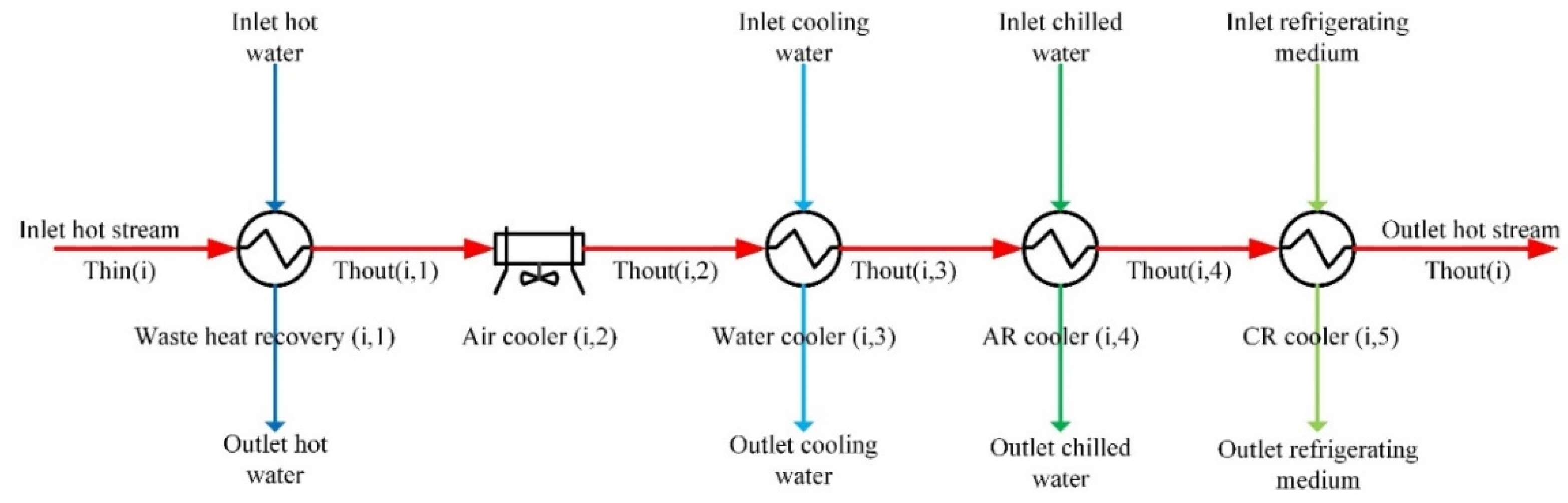
Therefore, in this work, a cascade cooling system containing waste heat recovery, air cooling, water cooling, absorption refrigeration, and compression refrigeration is proposed. Figure 1 is employed to show the structure of the cascade cooling system. Thout(i,1), Thout(i,2), Thout(i,3) and Thout(i,4) are the outlet temperatures of the hot streams of the waste heat recovery exchanger, air cooler, water cooler, and absorption refrigeration cooler, respectively. They are also the temperature breakpoints between the five heat exchangers. The breakpoints indicate the heat load distribution of the five heat exchangers and influence the capital cost and operation cost of heat exchangers. To obtain the optimal heat load distribution and the temperature breakpoints of hot streams, an optimization method combining Aspen Plus and a GA is proposed. Finally, a case study in a polysilicon enterprise was optimized in this work.

2. Problem Statement

Hot streams of a hydrochlorination plant in a polysilicon enterprise have high supply temperatures (more than 130 °C). These streams were cooled to target temperature by air cooler, water cooler, and compression refrigeration, originally. There are two problems with the original cooling process. Firstly, without waste heat recovery, the cooling duty of air/water cooling is large. Secondly, large amounts of energy will be consumed if the streams are cooled by compression refrigeration directly after water cooling. In view of these two problems, the cascade cooling system containing waste heat recovery, air cooling, water cooling, absorption refrigeration, and compression refrigeration was adopted.

The objective of this work is to determine the optimal heat load distribution of coolers and the optimal breakpoints of temperatures between waste heat recovery, air cooling, water cooling, absorption refrigeration, and compression refrigeration in terms of minimum total annual cost (TAC). The mathematical optimization model is established and solved, and the optimal design is based on several assumptions:

The specific heat capacities and film transfer coefficients of hot water, air, cooling water, chilled water, and ethylene glycol are constant. The film transfer coefficients of hot streams are constant. Due to the large temperature span of the hot stream, the specific heat capacity of the hot stream is not constant.

The heat loss during the heat exchange and the transportation of streams is ignored.

3. Model Formulation

3.1. Heat Exchanger Formulation

In Equation (1), Q is the heat load of the heat exchanger which is obtained through the simulation in Aspen; i and j represent the hot streams and cooling medium; and j = 1–5, respectively, represent hot water, air, cooling water, chilled water, and ethylene glycol. M and m are the mass flow rate of hot stream and cooling medium; I_in and I_out are the inlet and outlet specific enthalpy of hot stream; Cp_m is the specific heat capacity of the cooling medium; T_in and T_out are the inlet and outlet temperature of hot stream; tin and tout are the inlet and outlet temperature of the cooling medium.

$$Q(i,j)=M(i,j)\cdot (Iin(i,j)-Iout(i,j))=m(i,j)\cdot C{p}_{\mathrm{m}}(i,j)\cdot (tout(i,j)-tin(i,j))$$

(1)

For heat exchangers, dt_in and dt_out represent the temperature differences on both sides of the heat exchanger, and temperature differences should be greater than the minimum temperature approach difference preset for the heat exchanger [24], as shown in Equations (2) and (3).

$$d{t}_{\mathrm{in}}(i,j)=T_{in}(i,j)-t_{out}(i,j)\ge \Delta T_{\min }(i,j)$$

(2)

$$d{t}_{\mathrm{out}}(i,j)=T_{out}(i,j)-t_{in}(i,j)\ge \Delta T_{\min }(i,j)$$

(3)

The area of the heat exchanger can be calculated by Equation (4), in which hin and hout are film transfer coefficients of both sides of the heat exchanger.

$$A(i,j)=\frac{Q(i,j)}{{}^{K(i,j)\cdot \Delta T_{\mathrm{m}}(i,j)}}=\frac{Q(i,j)}{\frac{d{t}_{\mathrm{in}}(i,j)-d{t}_{\mathrm{out}}(i,j)}{{}^{\ln (d{t}_{\mathrm{in}}(i,j)/d{t}_{\mathrm{out}}(i,j))}}}\cdot (\frac{1}{h_{in}}+\frac{1}{h_{out}})$$

(4)

Equation (5) shows the capital cost of the heat exchanger; a, b, and c are the cost parameters. Then total capital cost of the heat exchangers in the cascade cooling system is shown as Equation (6).

$$C{C}_{\mathrm{HEX}}(i,j)=a+b\cdot A{(i,j)}^c$$

(5)

$$C{C}_{\mathrm{HEX}}={\displaystyle \sum C{C}_{\mathrm{HEX}}(i,j)}={\displaystyle \sum (a+b\cdot A{(i,j)}^c})$$

(6)

3.2. Pump Formulation and Pipe Formulation

Pumps are used to transport the cooling medium used in the cascade cooling system, such as hot water (HW), cooling water (CW), chilled water (CHW), and ethylene glycol (EG). The diameter of the pipe can be calculated by Equation (7), where ρ is the density of the cooling medium, and u is the flow velocity. It is assumed that the density of the cooling medium does not change with temperature.

$$D_{\mathrm{in}}(j)=\sqrt{\frac{4m(j)}{\pi \cdot \rho (j)\cdot u(j)}}$$

(7)

According to Equation (1), the mass flow rate of cooling medium can be calculated through Equation (8).

$$m(j)={\displaystyle \sum _{i=1}^n\frac{Q(i,j)}{C{p}_{\mathrm{m}}(i,j)\cdot (t_{out}(i,j)-t_{in}(i,j))}}$$

(8)

The capital cost and operation cost of the pump can be calculated through Equations (9) and (10), where α, β, γ are the parameters of the pump capital cost; Pe is the cost of the unit electricity; Hy is the annual operation time; and η_Pump is the pump efficiency [25].

$$C{C}_{\mathrm{Pump}}={\displaystyle \sum _{j\ne 2}^5(\alpha +\beta \cdot {(\frac{m(j)\cdot \Delta P(j)}{\rho (j)})}^{\gamma })}$$

(9)

$$O{C}_{\mathrm{Pump}}={\displaystyle \sum _{j\ne 2}^5(Pe\cdot Hy\cdot \frac{m(j)\cdot \Delta P(j)}{1000\cdot \rho (j)\cdot {\eta }_{\mathrm{Pump}}})}$$

(10)

In the above equation, ∆P is the pressure drop of the pump, which generally contains pipeline pressure drop and heat exchanger pressure drop, as shown in Equation (11).

$$\Delta P(j)=\Delta P_{\mathrm{PIPE}}(j)+\Delta P_{\mathrm{HEX}}(j)$$

(11)

The pressure drop of the pipeline is calculated by Equations (12)–(14), in which Re and f are Reynolds (Re) number and Fanning friction coefficient, μ is viscosity, and L is transmission distance. Fanning friction (the pipe is a hydraulically rough pipe) can be calculated through Equation (13) [26], and it is assumed that the Re number is between 3000 and 3 × 10⁶.

$$\mathrm{Re}=\frac{\rho \cdot D_{\mathrm{in}}\cdot u}{\mu }$$

(12)

$$f=0.0056+\frac{0.5}{{\mathrm{Re}}^{0.32}}$$

(13)

$$\Delta P_{\mathrm{PIPE}}=4\cdot f\cdot \frac{L\cdot \rho \cdot u^2}{2\cdot D_{\mathrm{in}}}$$

(14)

The pressure drop of the heat exchanger can be divided into tube and shell side pressure drop. Since the calculation of the shell side pressure drop is very complicated, and usually, the cooling medium flows in tube side and the hot stream flows in the shell side, only the pressure drop of the tube side is considered in this paper. The pressure drop is related to the constant K_t, the heat transfer area A, and the film heat transfer coefficient h_t. The constant K_t is related to the flow rate of the cooling medium m_t, viscosity μ_t, density ρ_t, heat conductivity κ_t, specific heat capacity Cp_t, and inner diameter Dt_in and outer diameter Dt_out of tube in the heat exchanger [27]. In this paper, except for the air cooler, other heat exchangers choose the same geometric shape and type, which is a counterflow single shell and single tube heat exchanger.

$$\Delta P_{\mathrm{HEX}}=\Delta P_{\mathrm{t}}=K_{\mathrm{t}}\cdot A\cdot h_{\mathrm{t}}^{3.5}$$

(15)

$$K_{\mathrm{t}}=\frac{D{t}_{\mathrm{in}}^{1/2}\cdot {\mu }_{\mathrm{t}}^{11/6}}{{0.023}^{2.5}\cdot {\rho }_{\mathrm{t}}\cdot {\kappa }_{\mathrm{t}}^{7/3}\cdot C{p}_{\mathrm{t}}^{7/6}\cdot m_{\mathrm{t}}}\cdot \frac{D{t}_{\mathrm{in}}}{D{t}_{\mathrm{out}}}\cdot {(\frac{{\mu }_{\mathrm{t}}}{{\mu }_{\mathrm{r}}})}^{-0.63}$$

(16)

In the calculation of the heat exchanger pressure drop, it is necessary to take the series and parallel structure of the heat exchanger into account. In general, the total pressure drop of the series structure is the sum of the pressure drop of all heat exchangers. The maximum pressure drop of the branch stream is taken as the pressure drop of the parallel structure [28]. In this paper, the heat exchanger network of the cooling medium and hot stream is in parallel structure.

In addition to considering the capital and operation cost of the pump for the cooling medium, the investment cost of the pipeline should also be calculated. The outer diameter D_out of the pipe is calculated from the inner diameter by Equation (17) [29], the constants in the equation are the model parameters for the calculation. Then the capital cost of the pipeline can be calculated by Equations (18)–(20) [29]. In the equation that follows, Wt is the weight of the pipe per unit length, Pcul is the investment cost of the pipe per unit length. In this paper, 80# steel pipes are selected, and A₁, A₂, A₃, and A₄ are the related cost parameters [29].

$$D_{\mathrm{out}}(j)=1.101\cdot D_{\mathrm{in}}(j)+0.006349$$

(17)

$$Wt(j)=1330\cdot D_{\mathrm{in}}^2(j)+75.18\cdot D_{\mathrm{in}}(j)+0.9268$$

(18)

$$Pcul(j)=A_1\cdot Wt(j)+A_2\cdot D_{\mathrm{out}}^2(j)+A_3+A_4\cdot D_{\mathrm{out}}(j)$$

(19)

$$C{C}_{\mathrm{PIPE}}={\displaystyle \sum _{j\ne 2}(L\cdot }Pcul(j))$$

(20)

3.3. Air Cooler Formulation

The ambient temperature influences the face velocity of the air cooler. T_ambient is the inlet air temperature of the air cooler. V_F and V_NF are the face velocity and actual face velocity of air cooler [30].

$$V_{\mathrm{NF}}=V_{\mathrm{F}}\cdot \frac{293}{273+T_{\mathrm{ambient}}}$$

(21)

Equation (22) is used to calculate the outside film heat transfer coefficient of the air cooler, which depends on its actual face velocity. In this work, it is assumed that the air flows through triangular pitch banks of finned tubes.

$$h_{\mathrm{a}}=218.9\cdot V_{\mathrm{NF}}^{0.718}$$

(22)

The energy consumption of the air cooler is related to the fan pressure drop. The air cooler fan pressure drop is related to the air mass flowrate and the number of bundles. Equations (23)–(25) were employed to calculate the fan pressure drop, where G represents the mass velocity rate, G_max is the maximum mass velocity when the air flows through the narrow part of air cooler, N_b is the number of bundles in air cooler, and f_friction is the friction factor.

$$G=V_{\mathrm{F}}\cdot {\rho }_{\mathrm{air}}$$

(23)

$$G_{\max }=2G$$

(24)

$$\Delta p_{\mathrm{air}}=9.8\cdot f_{\mathrm{friction}}\frac{N_{\mathrm{b}}\cdot G_{\max }^2}{2g{\rho }_{\mathrm{air}}}$$

(25)

Equation (26) represents the power consumption of the air cooler fan, V_air is the volumetric flow rate of air, and η_fan is the fan efficiency. Then the operation cost of air coolers can be calculated by Equation (27).

$$P_{\mathrm{fan}}(i,j)=\frac{\Delta p_{\mathrm{air}}\cdot V_{\mathrm{air}}(i,j)}{{\eta }_{\mathrm{fan}}}$$

(26)

$$O{C}_{\mathrm{AC}}={\displaystyle \sum _{j=2}{P}_{\mathrm{fan}}(i,j)\cdot Pe\cdot Hy}$$

(27)

3.4. Absorption Refrigeration Cycle Formulation

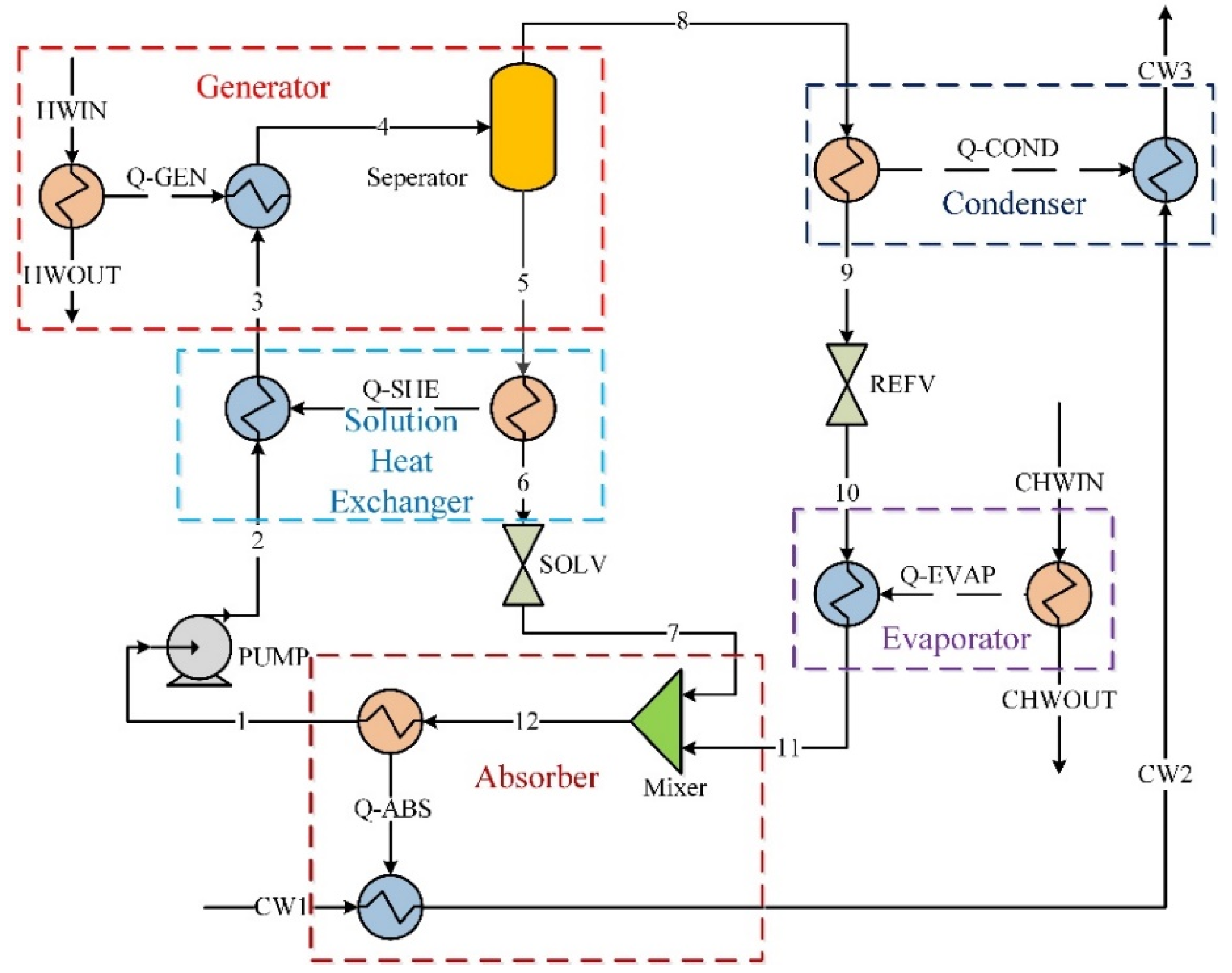
The absorption refrigeration cycle (ARC) used in the cascade cooling system is a traditional single-effect LiBr/H₂O absorption refrigeration cycle. It consists of a generator, condenser, throttle valve, evaporator, absorber, solution heat exchanger, and pump. Figure 2 shows the schematic diagram of the single-effect lithium bromide absorption refrigeration cycle [31].

This absorption refrigeration cycle is simulated in Aspen Plus, and the ELECNRTL Equation of State is selected for the electrolyte system [32]. The working fluid of this cycle is lithium bromide aqueous solution, whose original state (stream 1) is 36.62 °C, 800 Pa and the concentration is 0.58 (mass fraction). The absorbent is LiBr solution, and the refrigerant is pure water. The LiBr solution is heated by heat source (hot water from waste heat recovery) in the generator, and the refrigerant (water) is evaporated to steam and then condensed to saturated liquid in the evaporator and condenser. At the same time, the LiBr solution in the evaporator becomes a strong solution and flows into the absorber through a throttle. The saturated refrigerant liquid steps down to evaporating temperature by a throttle, then evaporates in the evaporator, resulting in a refrigeration effect. Then the saturated steam from the evaporator flows into the absorber and mixes with the strong LiBr solution. The strong solution absorbs the steam and becomes the weak solution as used in the beginning. Since the pressure of the generator is higher than that of the absorber, a pump is used to send the diluted solution back to the generator for the whole process to circulate.

Equation (28) expresses the calculation of the COP for the absorption refrigeration cycle, in which Q_AR-EAVP and Q_AR-GEN are the heat load of the evaporator and generator, respectively. The heat load of the generator should be the same as the total heat load of the waste heat recovery in the cascade cooling system. The heat load of the evaporator should also be the same as the total heat load of the absorption refrigeration in the cascade cooling system.

$$CO{P}_{\mathrm{AR}}=\frac{\mathrm{Cooling}\mathrm{capacity}\mathrm{generated}\mathrm{in}\mathrm{evaporator}}{\mathrm{Heat}\mathrm{absorbed}\mathrm{in}\mathrm{generator}}=\frac{Q_{\mathrm{AR}-\mathrm{EVAP}}}{Q_{\mathrm{AR}-\mathrm{GEN}}}$$

(28)

For simplicity of calculation, the capital cost of the absorption refrigeration machine is calculated by the sum of the capital costs of the heat exchangers and the working fluid pump. The operation cost is the operation cost of working fluid pump. The heat exchangers are the generator, condenser, evaporator, absorber, and solution heat exchanger. The area of these heat exchangers can be calculated by Equation (4). For the ARC model used in MATLAB, they can be found in reference [33]. Because all the models are the same, they are not listed in this paper.

Equations (31) and (32) are employed to calculate the capital cost and operation cost of the absorption refrigeration cycle. The calculation of the capital cost of the heat exchangers is the same as in Equation (5), and the capital and operation costs of pumps for working fluid and cooling water are same as Equations (9) and (10), while the mass flow rate of the working fluid M_LiBr and cooling water M_AR-CW can be calculated by Equations (31) and (32).

$$C{C}_{\mathrm{AR}}=C{C}_{\mathrm{AR}\text{-}\mathrm{GEN}}+C{C}_{\mathrm{AR}\text{-}\mathrm{COND}}+C{C}_{\mathrm{AR}\text{-}\mathrm{EVAP}}+C{C}_{\mathrm{AR}\text{-}\mathrm{ABS}}+C{C}_{\mathrm{AR}\text{-}\mathrm{SHE}}+C{C}_{\mathrm{Pump}\text{-}\mathrm{LiBr}}$$

(29)

$$O{C}_{\mathrm{AR}}=O{C}_{\mathrm{Pump}\text{-}\mathrm{LiBr}}$$

(30)

$$M_{\mathrm{LiBr}}=\frac{Q_{\mathrm{AR}\text{-}\mathrm{GEN}}}{q_{\mathrm{AR}\text{-}\mathrm{GEN}}}$$

(31)

$$M_{\mathrm{AR}\text{-}\mathrm{CW}}=\frac{Q_{\mathrm{AR}\text{-}\mathrm{ABS}}}{C{p}_{\mathrm{CW}}\cdot (T_{\mathrm{CW}2}-T_{\mathrm{CW}1})}$$

(32)

In Equation (31), q_AR-GEN is the heat load of the generator when the working fluid flow rate is 1 kg/s. In Equation (32), Q_AR-ABS is the heat load of the absorber. T_CW1 and T_CW2 are the inlet and outlet temperature of the cooling water in the absorber. T_CW2 can be calculated by Equation (33), in which T_CW3 is the outlet temperature of the cooling water in the condenser, and Q_AR-COND is the heat load of condenser.

$$\frac{T_{\mathrm{CW}2}-T_{\mathrm{CW}1}}{T_{\mathrm{CW}3}-T_{\mathrm{CW}2}}=\frac{Q_{\mathrm{AR}\text{-}\mathrm{ABS}}}{Q_{\mathrm{AR}\text{-}\mathrm{COND}}}$$

(33)

3.5. Compression Refrigeration Cycle Formulation

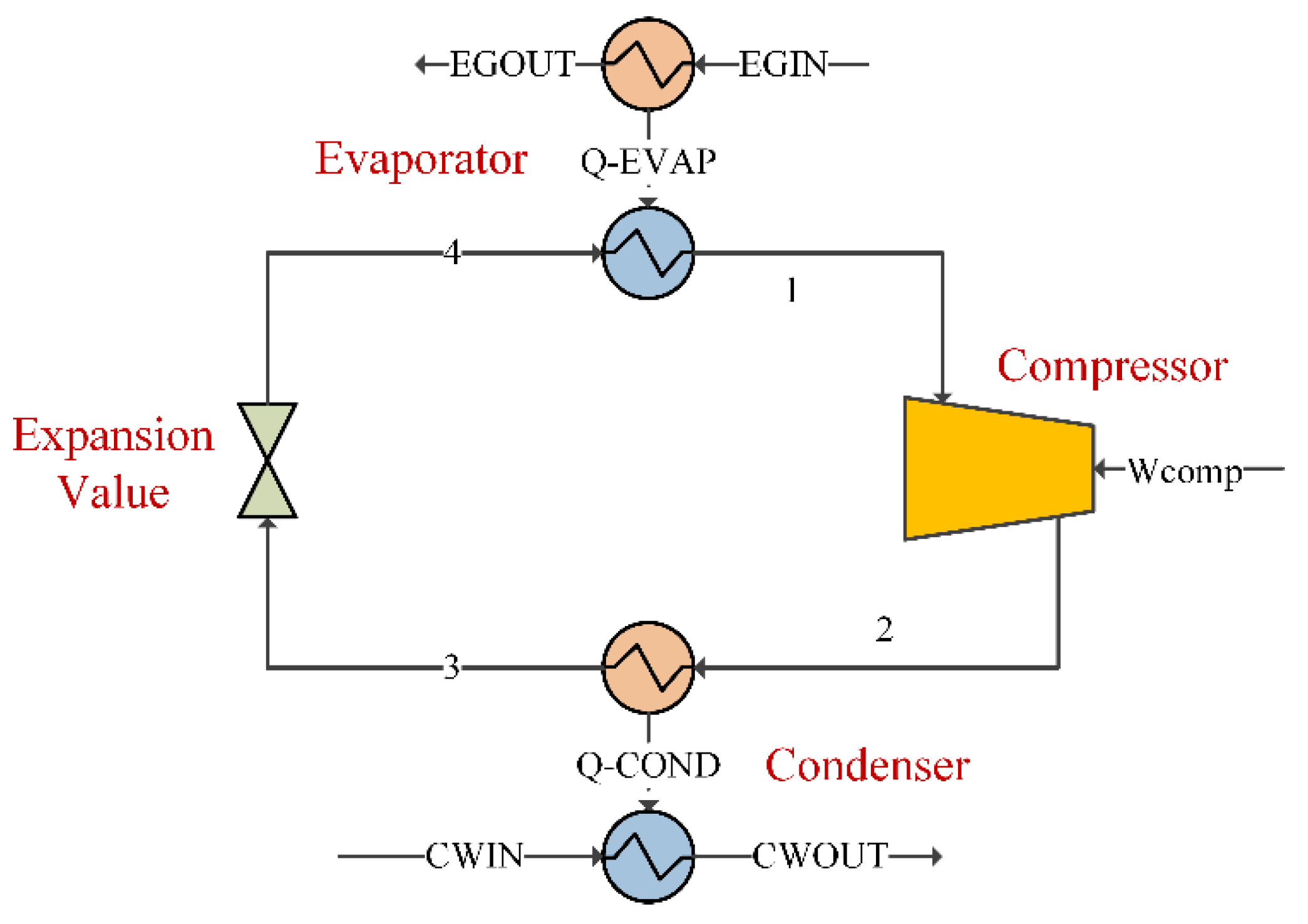
Traditional vapor compression refrigeration (VCR) is composed of an evaporator, a compressor, a condenser, and an expansion valve. This cycle is modeled in the Aspen Plus software, as shown in Figure 3. The REFPROP property method is adopted for simulation. R134a is selected as the refrigerant. For a compressor, the actual compression process is non-isentropic, and the parameter η_isen is used to describe the degree of non-isentropicity [34]. η_isen for the compressor is set as 0.7 during the simulation.

The COP of a vapor compression refrigeration cycle is an important system performance indicator. It represents the refrigeration effect per unit of compressor work required and is expressed by Equation (34) [35].

$$CO{P}_{\mathrm{CR}}=\frac{\mathrm{Refrigerating}\mathrm{effect} \left(\mathrm{Heat}\mathrm{load}\mathrm{of}\mathrm{evaporator}\right) }{\mathrm{Comprssion}\mathrm{work}\mathrm{of}\mathrm{the}\mathrm{compressor}}=\frac{Q_{\mathrm{CR}\text{-}\mathrm{EVAP}}}{W_{\mathrm{Comp}}}$$

(34)

In Equation (34), Q_CR-EVAP is the refrigeration effect which is equal to the total heat load of compression refrigeration coolers in the hot stream cooling process, W_Comp is the non-isentropic work of compressor. Operation cost of compressor can be calculated by Equations (35) and (36) [20]. In Equation (38), η_mech and η_e1 are mechanical efficiency and electrical efficiency. For the VCR model used in MATLAB, they can be found in reference [33]. Because all the models are the same, they are not listed in this paper.

$$W_{\mathrm{Comp}}=\frac{Q_{\mathrm{CR}\text{-}\mathrm{EVAP}}}{CO{P}_{\mathrm{CR}}}={\displaystyle \sum _{j=5}\frac{Q(i,j)}{CO{P}_{\mathrm{CR}}}}$$

(35)

$$O{C}_{\mathrm{Comp}}=\frac{W_{\mathrm{Comp}}}{{\eta }_{\mathrm{mech}}\cdot {\eta }_{\mathrm{el}}}\cdot Pe\cdot Hy$$

(36)

Equation (37) is used to express the capital cost of the compressor, where M_ref is the mass flowrate of the refrigerant. P_cond and P_evap are the operating pressure of the condenser and evaporator, respectively [36]. M_ref can be calculated by Equation (38), ∆H_EVAP is the enthalpy change of the evaporator when M_ref is 1 kg/s. According to the heat balance of the compression refrigeration cycle, the heat load of the condenser is given by Equation (39).

$$C{C}_{\mathrm{Comp}}=\left(\frac{573\cdot M_{\mathrm{ref}}}{0.8996-{\eta }_{\mathrm{isen}}}\right)\left(\frac{P_{\mathrm{cond}}}{P_{\mathrm{evap}}}\right)\ln \left(\frac{P_{\mathrm{cond}}}{P_{\mathrm{evap}}}\right)$$

(37)

$$M_{\mathrm{ref}}=\frac{Q_{\mathrm{CR}\text{-}\mathrm{EVAP}}}{\Delta H_{\mathrm{EVAP}}}$$

(38)

$$Q_{\mathrm{CR}\text{-}\mathrm{COND}}=Q_{\mathrm{CR}\text{-}\mathrm{EVAP}}+W_{\mathrm{Comp}}$$

(39)

Then the capital and operation cost of the compression refrigeration cycle are expressed by Equations (40) and (41).

$$C{C}_{\mathrm{CR}}=C{C}_{\mathrm{CR}\text{-}\mathrm{EVAP}}+C{C}_{\mathrm{CR}\text{-}\mathrm{COND}}+C{C}_{\mathrm{Comp}}$$

(40)

$$O{C}_{\mathrm{CR}}=O{C}_{\mathrm{Comp}}$$

(41)

3.6. Cooling Tower Formulation

Cooling towers are usually present wherever water is used as a cooling medium, there are many factors that influence the performance and cost of a cooling tower, such as atmospheric pressure, local air wet bulb temperature and air humidity, cooling water flowrate, and inlet/outlet temperature, etc. To formulate the cooling tower, the following definitions are necessary.

First, the operation cost of the cooling tower includes the cooling tower fan cost, water treatment cost, make-up water cost, and blowdown treatment cost. The constants in Equation (42) are the cost parameters for the calculation.

$$O{C}_{\mathrm{CT}}=O{C}_{\mathrm{fan}\text{-}\mathrm{tower}}+110\cdot ft+Pw\cdot Hy\cdot M_{\mathrm{makeup}}+1138\cdot B_{\mathrm{blowdown}}$$

(42)

In Equation (42), OC_fan-tower is the operation cost of the tower fan, ft is the total flowrate of the cooling water, M_makeup is the flowrate of make-up water, B_blowdown is the flowrate of water blowdown, and Pw is the price of fresh water [37]. OC_fan-tower can be calculated by Equation (43).

$$O{C}_{\mathrm{fan}\text{-}\mathrm{tower}}=\frac{Pe\cdot Hy\cdot C_{\mathrm{factor}}\cdot F_{\mathrm{air}}}{{\eta }_{\mathrm{fan}\text{-}\mathrm{tower}}}$$

(43)

In Equation (43), C_factor is the fan factor. To draft each 18,216.44 m³/h of air, 1 kW is required. F_air is the air mass flowrate of the cooling tower. η_fan-tower is the fan efficiency.

Mass flowrate of air, make-up water and blowdown water are shown in Equations (44)–(46). E_vop is the amount of water evaporation, w_in and w_out are the inlet and outlet humidity of air, and π_c is the cycle of concentration.

$$F_{\mathrm{air}}=\frac{E_{\mathrm{vop}}}{w_{\mathrm{out}}-w_{\mathrm{in}}}$$

(44)

$$M_{\mathrm{makeup}}=E_{\mathrm{vop}}\cdot \frac{E_{\mathrm{vop}}}{{\pi }_{\mathrm{c}}-1}$$

(45)

$$B_{\mathrm{blowdown}}=\frac{E_{\mathrm{vop}}}{{\pi }_{\mathrm{c}}-1}$$

(46)

The amount of water evaporation is related to the cooling tower range and water flowrate. Range is the difference between the cooling tower inlet temperature T_cin and outlet temperature T_cout.

$$E_{\mathrm{vop}}=0.00153\cdot ft\cdot Range$$

(47)

$$Range=T_{\mathrm{cin}}-T_{\mathrm{cout}}$$

(48)

The cooling tower inlet air humidity is the local air humidity. The outlet air humidity is calculated by Equations (49)–(51). MW_w and MW_air are water and air molecular weight, P_s and P_a are vapor pressure and local atmospheric pressure, and T_mean is the mean temperature of the cooling tower [38].

$$w_{\mathrm{out}}=\frac{M{W}_{\mathrm{w}}}{M{W}_{\mathrm{air}}}\cdot \frac{P_{\mathrm{s}}}{P_{\mathrm{a}}-P_{\mathrm{s}}}$$

(49)

$$Ln{P}_{\mathrm{s}}=23.1-\frac{4111}{T_{\mathrm{mean}}+237.7}$$

(50)

$$T_{\mathrm{mean}}=\frac{T_{\mathrm{cout}}+T_{\mathrm{cin}}}{2}$$

(51)

Besides, the capital cost of the cooling tower is determined by many factors. Equation (52) is the capital cost of the cooling tower, in which Approach is temperature difference between the cooling tower outlet temperature and the air bulb temperature T_wb.

$$C{C}_{\mathrm{CT}}=746.74\cdot f{t}^{0.79}\cdot Rang{e}^{0.57}\cdot Approac{h}^{-0.9924}+{(0.022\cdot T_{\mathrm{wb}}+0.39)}^{2.447}$$

(52)

$$Approach=T_{\mathrm{cout}}-T_{\mathrm{wb}}$$

(53)

In this work, there should be three cooling towers because of the different cooling waters for different cooling requirements, one for the cooling of the hot streams, one for the cooling of the absorber and condenser of the ARC, and one for the cooling of the condenser of the CRC.

3.7. Objective Function

The objective of this work is to determine the optimal heat load distribution of the cascade cooling system with minimizing TAC. TAC includes the heat exchanger capital cost, capital and operation costs of pumps, operation costs of air coolers, capital and operation costs of the absorption refrigeration cycle, capital and operation costs of the compression refrigeration cycle, and capital and operation costs of the cooling towers.

$$\begin{array}{ll}TAC\hfill & =Af\cdot TCC+TOC\hfill \\ \hfill & =Af\cdot \left(C{C}_{\mathrm{HEX}}+C{C}_{\mathrm{Pump}}+C{C}_{\mathrm{PIPE}}+C{C}_{\mathrm{AR}}+C{C}_{\mathrm{CR}}+C{C}_{\mathrm{CT}1}+C{C}_{\mathrm{CT}2}+C{C}_{\mathrm{CT}3}\right)\hfill \\ \hfill & +\left(O{C}_{\mathrm{AC}}+O{C}_{\mathrm{Pump}}+O{C}_{\mathrm{AR}}+O{C}_{\mathrm{CR}}+O{C}_{\mathrm{CT}1}+O{C}_{\mathrm{CT}2}+O{C}_{\mathrm{CT}3}\right)\hfill \end{array}$$

(54)

In the objective function above, TCC, TOC, and TAC are the total capital cost, total operation cost, and total annual cost of the cooling system, respectively. Af is the annualized factor of capital cost which is calculated as Equation (55), where I is the annual interest rate and n is the lifetime of the equipment in terms of years.

$$Af=\frac{I\cdot {(1+I)}^n}{{(1+I)}^n-1}$$

(55)

4. Solution Technique Employed

In this work, Aspen Plus was combined with MATLAB to solve the problem. Aspen Plus was used to simulate the cooling process of hot streams, the LiBr/H₂O absorption refrigeration cycle, and the compression refrigeration cycle, and it provided data for MATLAB calculations. MATLAB was used to assign and read data from Aspen, as well as to control Aspen to open, run, and close [39]. They were combined through an interface program based on ActiveX technology. The interface process between Aspen and MATLAB is shown in Figure 4.

Because the model contains large amounts of nonlinear terms, a heuristic algorithm such as a genetic algorithm (GA) can solve this problem more effectively. GA simulates natural selection and a genetic mechanism for optimization. It is an effective parallel, random, adaptive search algorithm, which has less mathematical requirements for the problem to be solved. It is a black-box solution. The remarkable characteristics of the genetic algorithms are their inner parallelism and their ability to search for global optimization. The combination of GA and process simulation software not only eliminates the need to establish rigorous mathematic models for complex chemical processes, but also enables global optimization for nonlinear, multivariate and multi-objective problems [40].

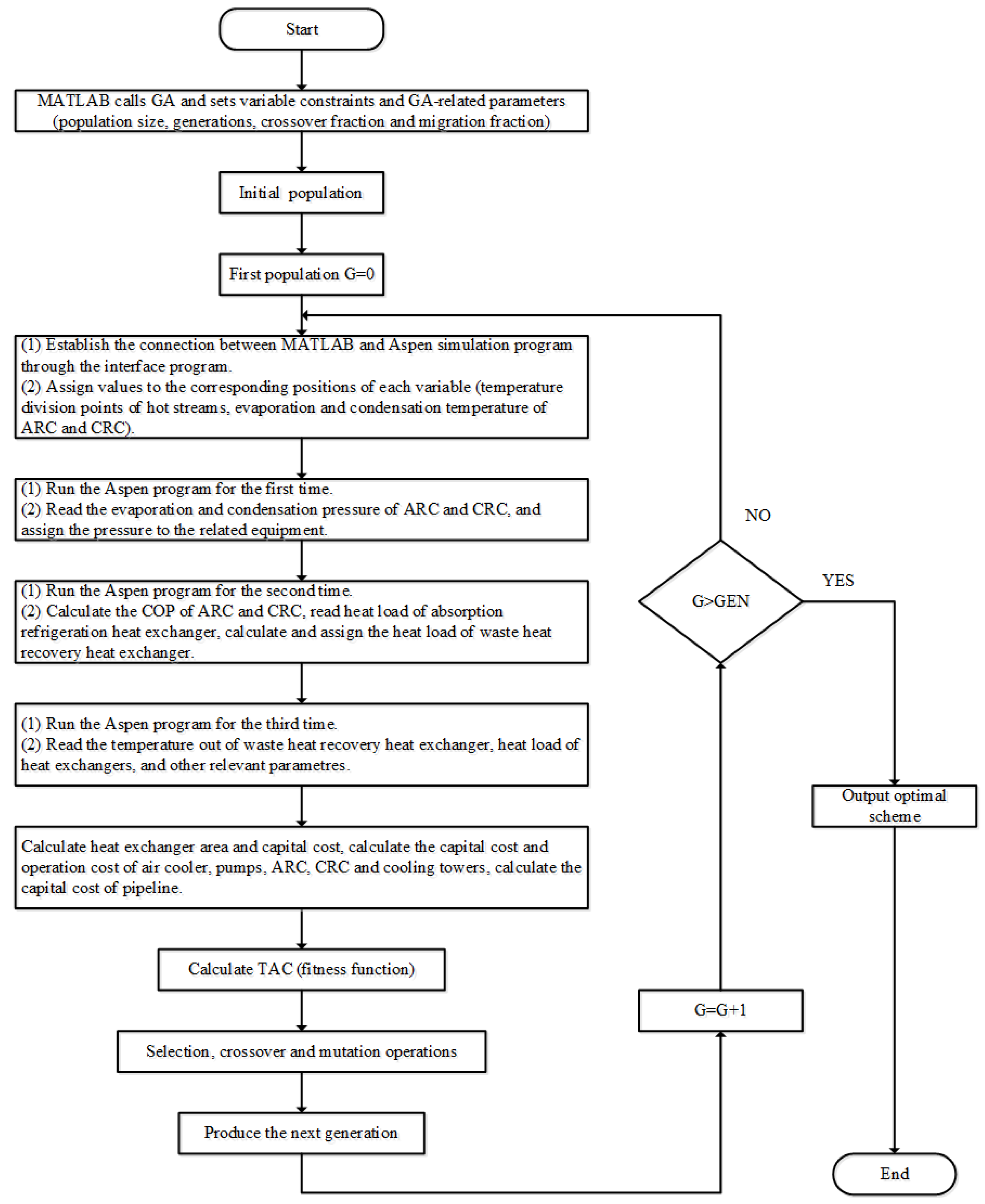
Figure 5 is used to show the block diagram of the optimization program which combines both Aspen Plus and GA. The evaporation and condensation temperatures of ARC and CRC determine the operating pressure of the cycles when simulating. In addition, the cascade cooling system determines the amount of waste heat recovered according to the actual refrigeration requirements. Therefore, the Aspen program needs to be run three times in the optimization. In the first run, evaporation and condensation pressure are calculated according to the input evaporation and condensation temperature. In the second run, the COP of ARC and CRC are calculated after the evaporation and condensation pressure are re-assigned. In the third run, according to the COP calculated and the heat load of the absorption refrigeration heat exchanger, the heat load of the waste heat recovery heat exchanger is recalculated and re-assigned, so as to determine the hot stream temperature out of the waste heat recovery heat exchanger and the heat load of the air cooler.

The variable of the optimization procedure is the temperature in the cascade cooling system, including the breakpoint temperatures of the hot stream cooling process, the evaporation and condensation temperature of refrigeration cycle, the inlet and outlet temperature of cooling medium (e.g., hot water, air, cooling water, chilled water, and ethylene glycol solution). The objective function of optimization is the total annual cost of the system, and the termination condition of the GA is to reach the maximum genetic algebra (GEN).

5. Case Study

To verify the effectiveness of the cascade cooling system, a case study taken from a polysilicon enterprise is employed. The hot streams are the reaction tail gas of a hydrochlorination reaction unit of silicon tetrachloride in the polysilicon enterprise, which are composed of HCl (hydrogen chloride), DCS (dichlorosilane), TCS (trichlorosilane), STC (silicon tetrachloride), and H₂ (hydrogen). In the reactive tail gas treatment process, the tail gas is first used to preheat the raw material STC of the reaction, then it is cooled by series cooling and refrigeration methods. The chlorosilane is condensed down to realize the separation and recycling of H₂ and HCl. In this paper, only the cooling process of hot streams is taken into consideration. The hot streams data is shown in

Table 1. Hot stream data.

$\mathbf{Hot} \mathbf{Stream} \left(\mathit{i}\right)$	Ts (°C)	Tt (°C)	M (kg·s−1)	hH (W·(m2·°C)−1)	Components (Mass Fraction)
H1	132.19	−5.8	34.0	500	HCl: 0.00036, DCS: 0.00615, TCS: 0.19751, STC: 0.78222, H2: 0.01376
H2	131.82	−6.7	33.5	500	HCl: 0.00036, DCS: 0.00619, TCS: 0.19828, STC: 0.78122, H2: 0.01394
H3	131.82	−7.1	33.4	500	HCl: 0.00037, DCS: 0.00619, TCS: 0.19828, STC: 0.78122, H2: 0.01394

, Ts and Tt are the supply temperature after heat exchange with STC and target temperature of hot streams respectively. h_H is the film transfer coefficient of hot streams, but the specific heat capacity of the hot stream is not a constant because it varies with temperature.

The hot streams have relatively high supply temperature (more than 130 °C) and low target temperature (less than 0 °C). The cooling mediums used in the cooling process are hot water (HW), air (AIR), cooling water (CW), chilled water (CHW), and ethylene glycol solution (EG), respectively. The cooling medium data is shown in

Table 2. Cooling medium data.

$\mathbf{Cooling} \mathbf{Medium} \left(\mathit{j}\right)$	tin (°C)	tout (°C)	ρ (kg·m−3)	Cp (kJ·(kg·°C)−1)	μ (Pa·s)	κ (W·(m·K)−1)	hC (W·(m2·°C)−1)
1 (HW)	90~110	100~120	950	4.200	0.0003	0.68	2500
2 (AIR)	35~35	60~65	1.169	1.004	0.0011	0.024	475.93
3 (CW)	20~25	45~50	995	4.182	0.001	0.62	2500
4 (CHW)	7~12	12~17	1000	4.182	0.0015	0.57	2500
5 (EG)	−15~−10	−5~0	1082.45	2.582	0.007	0.39	2500

, tin and tout are the inlet and outlet temperature of the cooling medium in the heat exchangers, ρ is the density of cooling medium, Cp is the specific heat capacity, μ is viscosity, κ is thermal conductivity, and h_C is the film transfer coefficient. Since the inlet and outlet temperature of the cooling medium are also the optimization variables, their value ranges are listed in the table. In addition, hc is selected through industrial experience.

Some other economic parameters and physical parameters of the case study are presented in

Table 3. Economic parameters of case study.

Items	Data
Air coolers capital cost (USD) [1]	4778·A0.525
Other heat exchangers capital cost (USD) [43]	8500 + 409·A0.85
Pump capital cost (USD)	8600 + 7310(M·∆P/ρ)0.2
Air cooler fan efficiency	70%
Cooling tower fan efficiency	70%
Pump efficiency	70%
Compressor isentropic efficiency	70%
Compressor mechanical efficiency	80%
Compressor electrical efficiency	90%
Price of electricity (USD·kWh−1)	0.15
Price of fresh water (USD·t−1)	0.5
Plant operation time (h·y−1)	8000
Plan lifetime (y)	5
Interest rate	15%
Annualized factor	0.298

and

Table 4. Other physical parameters and constrains of case study.

Items		Data
Minimum temperature approach difference of heat exchanger ΔTmin	Waste heat recovery cooler	10 °C
	Water cooler/air cooler	10 °C
	Absorption refrigeration cooler	3 °C
Allowable outlet temperature of air cooler		50~65 °C
Allowable outlet temperature of water cooler		25~35 °C
Allowable outlet temperature of absorption refrigeration heat exchanger		10~15 °C
Ambient temperature Tambient		25 °C
Wet bulb temperature Twb		12 °C
Air saturated humidity at wet bulb temperature		0.011 kgw·kga−1
Atmospheric pressure		101,325 Pa
Air cooler face velocity		3 m·s−1
Air cooler friction factor		0.95
Air cooler number of bundles		4
Cycle of concentration		4
ARC condensation temperature		35~45 °C
ARC evaporation temperature		5~10 °C
ARC cooling water initial temperature		30~32 °C
ARC cooling water final temperature		32~42 °C
CRC condensation temperature		35~45 °C
CRC evaporation temperature		−20~−15 °C
CRC cooling water initial temperature		27~37 °C
CRC cooling water final temperature		32~42 °C

, respectively [41,42].

5.1. The Base-Case Cooling System of Hot Streams

In this work, the cooling system containing air cooling, water cooling, and compression refrigeration were optimized as a base case. The NRTL-RK property method was selected for the simulation of the hot streams cooling process in Aspen Plus, because the hot stream is a weakly polarized system. The base-case cooling system of hot streams is shown in Figure 6. The inlet and outlet air temperature in the air cooler are 20 °C and 60 °C, and the inlet and outlet air temperatures in the cooling tower are 20 °C and 35 °C, respectively.

It can be seen from Figure 6 that the inlet and outlet temperature of the cooling water are 20 °C and 47 °C, and the temperature breakpoints of air cooler, water cooler, and compression refrigeration cooler are 58 °C and 30 °C, which are the minimum allowable outlet temperatures of air cooler and water cooler. The purpose is to reduce the heat load of compression refrigeration as much as possible, so as to reduce the operation cost of the compression refrigeration cycle. At the same time, it can reduce the flow rate of the cooling water as well as the costs of related pumps and pipelines.

The operation cost of the compression refrigeration cycle in this case is USD 2,514,212·y⁻¹, representing 55.80% of the total annual cost and 81.55% of the total operation cost of the cooling system. In addition, the total heat load of the air cooler is 19,829 kW, in which a large amount of low-grade waste heat available for recovery is directly released into the environment. The total heat load of the compression refrigeration heat exchanger is 4226 kW, and the power of the compressor is 1509 kW. This process will consume a lot of electric energy, resulting in the large operation cost of the compression refrigeration cycle. In the base-case cooling system, there are problems such as the loss of low-grade waste heat resources and large energy consumption of refrigerating. How to recover and utilize low-grade waste heat and reduce cooling energy consumption of the cooling system are important questions for improving the economy of the cooling system.

5.2. The Cascade Cooling System of Hot Streams

The cascade cooling system of hot streams consists of waste heat recovery, air cooling, water cooling, absorption refrigeration, and compression refrigeration. In this system, hot water is used as an intermediate medium to recover waste heat from hot streams and drives the LiBr/H₂O absorption refrigeration cycle, providing sub-ambient cooling capacity for the hot streams cooling process. In this way, the heat load of air cooling, water cooling, and compression refrigeration can be reduced, as well as the operation cost of the compression refrigeration cycle.

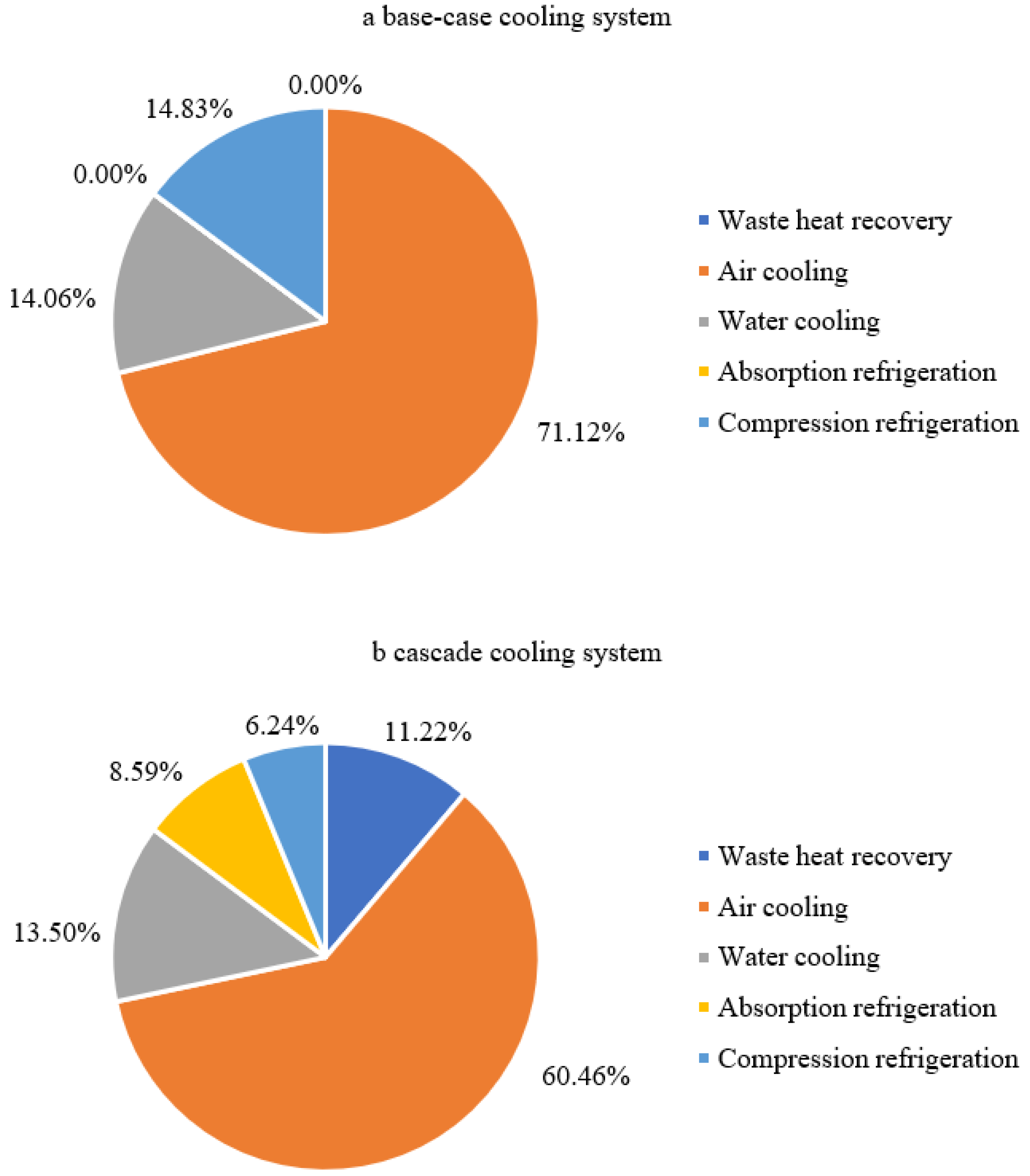
Figure 7a,b is used to indicate the heat load distribution of the base-case and cascade cooling systems, taking hot stream H1 as an example. It can be seen from Figure 7a that large amounts of low-grade waste heat are released into the environment form air coolers, and the heat load of compression refrigeration occupies about 15% of the total heat load, resulting in a large energy consumption of the compressor, i.e., the operation cost of the compressor is large. Compared to the base-case cooling system, the cascade cooling system can recover 11.22% of waste heat and provides 8.59% of sub-ambient cooling capacity through the absorption refrigeration cycle. The heat load of compression refrigeration is reduced by 8.59%, which means a lower operation cost of the compressor.

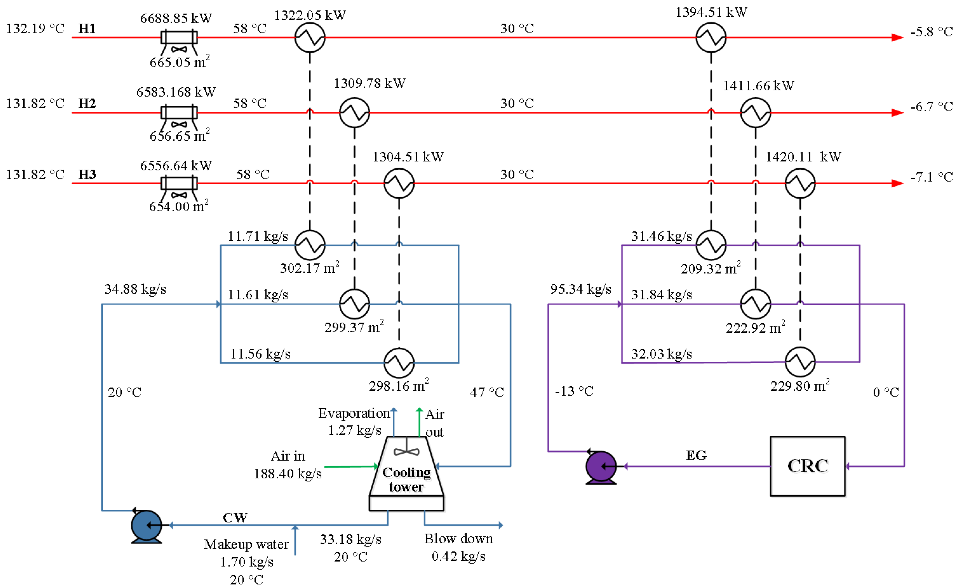
The optimal cascade cooling system of hot streams after optimization is shown in Figure 8. The heat load distribution and temperature breakpoints, the temperature of the cooling medium, and the area of the heat exchangers are also indicated.

As can be seen from Figure 6 and Figure 8, the temperature break point between air cooling and water cooling in the base-case and cascade cooling systems has a small change of only 1 °C. In the cascade cooling system, the temperature break points between air cooling, absorption refrigeration, and compression refrigeration are 30 °C and 10 °C, respectively. The aim was to reduce the heat load of compression refrigeration as much as possible, thus reducing the energy consumption and cost associated with compression refrigeration. In the hot stream cooling process, the cascade cooling system recovered 3139 kW of low-grade waste heat and then generated a refrigerating capacity of 2404 kW through the absorption refrigeration cycle, accounting for 56.87% of the total refrigerating capacity, which effectively reduced the refrigeration load of the compression refrigeration cycle.

A comparison of the system costs between the base case and the cascade cooling system is shown in

Table 5. Comparison of results between base-case and cascade cooling systems.

Items	Base-Case Cooling System	Cascade Cooling System
TAC (USD·y−1)	4,505,811	3,574,786
TCC (USD)	4,773,854	6,029,170
TOC (USD·y−1)	3,083,203	1,778,093
CCHEX (USD)	760,560	970,190
CCPUMP (USD)	203,819	384,554
CCPIPE (USD)	2,894,782	3,961,743
CCAR (USD)	-	208,396
CCCR (USD)	893,692	481,577
CCCT1 (USD)	10,267	10,026
CCCT2 (USD)	-	7282
CCCT3 (USD)	10,734	5403
OCPUMP (USD·y−1)	188,834	267,727
OCAC (USD·y−1)	77,193	65,583
OCAR (USD·y−1)	-	68
OCCR (USD·y−1)	2,514,212	1,178,940
OCCT1 (USD·y−1)	78,092	78,946
OCCT2 (USD·y−1)	-	98,258
OCCT3 (USD·y−1)	224,873	88,572
Fan power (kW)	316	276
Compressor power (kW)	1509	982

. Compared to the base case, the TAC of the cascade cooling system was reduced by USD 931,025·y⁻¹, primarily due to the reduction of USD 1,305,110·y⁻¹ in the TOC of the system. The addition of waste heat recovery and an absorption refrigeration heat exchanger reduced the heat load of air cooling and the compression refrigeration greatly, reducing the operation cost of the air cooler by USD 11,610·y⁻¹ and of the compression refrigeration cycle by USD 1,335,272·y⁻¹, which also greatly reduced the total annual cost of the system. However, the operation cost of the compression refrigeration cycle still accounted for 32.98% of the TAC and 66.30% of the TOC, indicating that the compression refrigeration cycle was still the main energy consumption part of the cascade cooling system. The TCC of the system increased by USD 1,255,316, mainly because of the additional investment in an absorption refrigeration cycle, waste heat recovery heat exchangers, absorption refrigeration heat exchangers, and relevant pumps and pipelines. Compared to the base case, the capital cost of the heat exchanger in a cascade cooling system increased by USD 209,630, and the total area of heat exchangers increased from 3537 m² to 4314 m².

The parameters related to the refrigeration cycle in the base case and the cascade cooling system are shown in

Table 6. Parameters of the refrigeration cycle.

Items	CRC in Base Case	ARC in Cascade System	CRC in Cascade System
COP	2.8016	0.7657	2.5768
Generating temperature (°C)	-	110	-
Evaporating temperature (°C)	−15	5	−17
Condensing temperature (°C)	35	45	36
Evaporating pressure (Pa)	163,940	873	150,837
Condensing pressure (Pa)	886,981	9590	911,849
Refrigerant flow rate (kg·s−1)	30.05	7.18	13.22
Secondary refrigerant flow rate (kg·s−1)	95.34	71.53	35.64
Cooling water inlet temperature (°C)	27	30	27
Cooling water outlet temperature (°C)	32	42	33
Cooling water flow rate (kg·s−1)	274.39	112.24	100.88

. Compared with the base case, the COP of the compression refrigeration cycle decreased. As a result of the reduction of the compression refrigeration heat load, the flow rates of the refrigerant, secondary refrigerant, and cooling water required were greatly reduced. The capital cost of CRC was reduced by USD 412,115, the operation cost of CRC was reduced by USD 1,335,272·y⁻¹, and the corresponding pump and cooling tower costs were reduced. The cascade cooling system used both absorption refrigeration and compression refrigeration to achieve the refrigerating purpose, the cooling water used was 213.1 kg·s⁻¹, which is 61.3 kg·s⁻¹ less than that of the base case only using compression refrigeration.

The base case consumed 18,969,640 kWh of electricity per year, and the cascade cooling system consumed 11,168,820 kWh·y⁻¹. Using the cascade cooling system saved 7,800,820 kWh of electricity per year and about 3120 t of standard coal, and it reduced 7778 t of carbon dioxide emissions.

In order to explore the optimal structure of cascade cooling system under different industrial conditions, the cascade cooling system of the same case was optimized in different areas; Nanchang and Xi’an were selected respectively. Unlike Xi’an, where water is extremely scarce, Nanchang is rich in water; hence, the price of fresh water in Nanchang is much lower than in Xi’an, but the electric charge is slightly higher. The costs of the cascade cooling system in two places after optimization are shown in

Table 7. Comparison of cascade cooling system results in different regions.

Items	Nanchang	Xi’an
Pe (USD·kWh−1)	0.096	0.083
Pw (USD·t−1)	0.344	0.843
TAC (USD·y−1)	2,941,456	2,836,840
TCC (USD)	6,063,125	5,976,545
TOC (USD·y−1)	1,134,644	1,055,830
CCHEX (USD)	968,291	981,735
CCPUMP (USD)	385,700	384,757
CCPIPE (USD)	213,689	208,396
CCAR (USD)	447,170	447,170
CCCR (USD)	10,135	9783
CCCT1 (USD)	6827	7282
CCCT2 (USD)	5189	5189
CCCT3 (USD)	4,026,123	3,932,234
OCPUMP (USD·y−1)	174,547	148,380
OCAC (USD·y−1)	50,212	36,624
OCAR (USD·y−1)	43	37
OCCR (USD·y−1)	732,608	633,401
OCCT1 (USD·y−1)	53,929	74,645
OCCT2 (USD·y−1)	68,128	99,737
OCCT3 (USD·y−1)	55,178	66,006

.

According to the results, the TAC of Nanchang system is USD 168,142·y⁻¹ higher than that of Xi’an system, the TOC is USD 156,558·y⁻¹ higher than that of the Xi’an system, and the TCC is only USD 38,872·y⁻¹ higher. The main reason is that the electricity price in Nanchang is higher than that in Xi’an; hence, the operation cost of compression refrigeration cycle is USD 186,324·y⁻¹ higher, and the operation cost of the pumps is 24,096 USD·y⁻¹ higher than that in Xi’an. Because the fresh water price in Xi’an is much higher than that in Nanchang, the operation costs of cooling towers in the Xi’an system are higher than those in the Nanchang system. It also can be seen from the results that the fresh water price has a small impact on the system cost, while the electricity price has a greater influence on the system cost.

5.3. The Sensitivity Analysis for the Cascade Cooling System

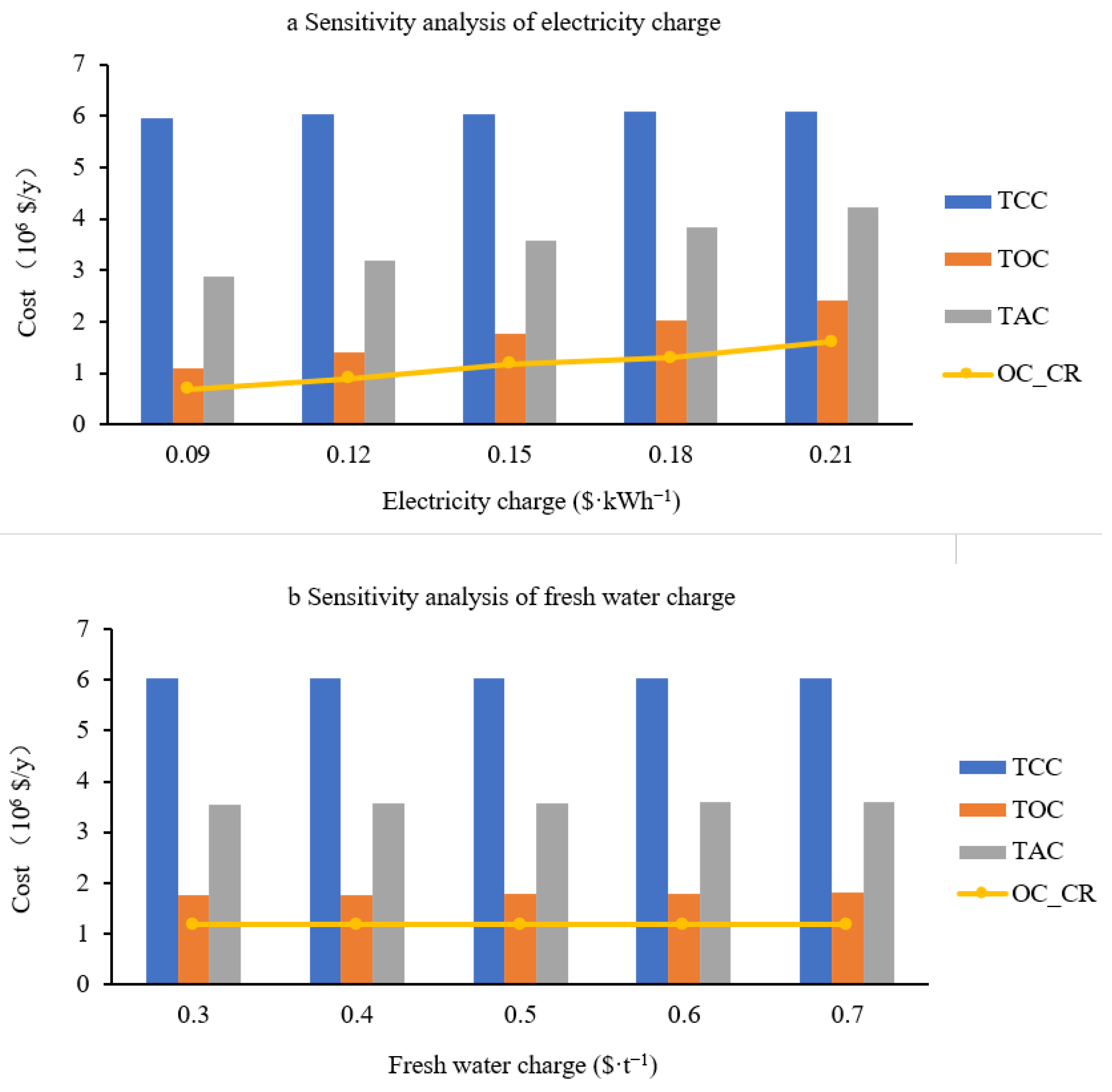
In this section, sensitivity analyses of the electricity charge and fresh water charge were carried out to study their influences on the cascade cooling system. The influences of the electricity charge and fresh water charge on the TCC, TOC, and TAC are shown in Figure 9a,b.

Both the electricity charge and the fresh water charge had little influence on TCC. TOC and TAC increased with the electricity charge, while they increased a little with the fresh water charge. That is because the electricity charge is related to all the operation costs, especially the operation cost of the compressor, but the fresh water charge is only related to the operation cost of the cooling tower. Fresh water was only used as the make-up water in the cooling tower, and its mass flowrate is small in this system; hence, it had little influence on the cost of the system. Figure 9 also shows the change of the operation cost of the compression refrigeration cycle in the cascade cooling system with electricity and fresh water prices. It increased with the increase of the electric charge, while it changed very little with the fresh water charge.

Taking the impact of electric charge and fresh water charge on the total cost of the system into account, as well as the comparative analysis of cascade cooling systems in different regions above, the cascade cooling system proposed in this paper is less dependent on water resources, and can be applied in areas with abundant and scarce water resources. However, it has more advantages in areas with a low electricity price. It is noted that the environment temperature was assumed to be the same in all situations.

5.4. The Comparison of Optimization Method with Using MATLAB Only

In this paper, Aspen and MATLAB were combined to optimize the cascade cooling system. The shortcoming of this optimization method is its low computational efficiency, mainly because the interaction process between Aspen and MATLAB consumes too much time. There is another optimization method to solve the problem, which uses MATLAB only. In this method, the process simulated in Aspen, such as the cooling process of hot streams, the absorption refrigeration cycle, and the compression refrigeration cycle are modeled and calculated in MATLAB. The method using MATLAB can greatly save computation time and improve optimization efficiency.

It can be seen from

Table 8. Parameter comparison of the optimization methods.

	Aspen and MATLAB	MATLAB
Population size	30	300
Maximum generation	500	5000
Computation time (s)	340,471	1884

that the population size and maximum generation in the method using MATLAB is 10 times higher than that in the method using Aspen and MATLAB. However, the computation time of the method using Aspen and MATLAB is 94.57 h, which is 180 times the computation time of the method using MATLAB. Meanwhile, in the base-case cooling system, the number of variables is 16, but the computation time using Aspen and MATLAB is 72.39 h. Thus, the reduction of the number of variables is helpful to improve the computational efficiency of the method using Aspen and MATLAB, but the main reason for the low efficiency of this method is still that the interaction between Aspen and MATLAB consumes too much time.

The method combining Aspen and MATLAB directly models the processes. By selecting the appropriate physical property method, the required data, such as temperature, pressure, and heat load, can be read directly after simulation and calculation. This method is intuitive and convenient. The method using MATLAB only requires not only the establishment of the thermodynamic model of the processes, but also the modeling and solving of the related physical properties of the hot streams and refrigeration working medium, which is a complicated and cumbersome process.

The modeling of the hot streams cooling process, absorption refrigeration cycle, and compression refrigeration cycle is different between the two optimization methods, which results in different calculation results. Aspen and MATLAB combined use a series heat exchanger model to model the cooling process of the heat streams; the heat load of heat exchangers can be obtained directly through the simulation and calculation of Aspen after assigning the outlet temperature of the heat exchanger. The method using only MATLAB calculates the heat load through the enthalpy difference between the inlets and outlets of heat exchangers. Although the enthalpy calculation equation of the hot streams is obtained through the data fitting from Aspen, there is a certain error between the fitting equation and the simulation data; hence, the calculation result is not as accurate as that in Aspen.

Table 9. Heat exchanger load of cascade cooling system (H1).

Heat Exchanger Load (kW)	Waste Heat Recovery	Air Cooling	Water Cooling	Absorption Refrigeration	Compression Refrigeration	Total Heat Load
Aspen and MATLAB	1055.07	5686.41	1269.42	807.85	586.67	9405.41
MATLAB	1062.51	5692.98	1402.14	780.49	560.58	9498.69

shows the heat load of the heat exchangers obtained by the two optimization methods which takes H1 as an example. The total heat load of Aspen and MATALB is 9,405.41 kW, and that of MATLAB is 9,498.69 kW. This constitutes an increase of 93.28 kW, and the margin of error is 0.99%. Meanwhile, compared to Aspen and MATLAB, although the temperature breakpoints between water cooling, absorption refrigeration, and compression refrigeration are the same, the heat load of the heat exchangers in the method using MATLAB is smaller than that in Aspen and MATLAB. The heat load of the absorption refrigeration heat exchanger is reduced by 27.36 kW, and the error is 3.39%. The heat load of the compression refrigeration heat exchanger is reduced by 26.08 kW with an error of 4.45%.

In addition, the calculations of the ARC and CRC, as well as the physical properties of the refrigeration working medium in the two optimization methods are different. Therefore, the calculation results of the two optimization methods are different.

Table 10. Comparison of optimization results of cascade cooling system with different methods.

Items	Aspen and MATLAB	MATLAB
TAC (USD·y−1)	3,574,786	3,475,097
TCC (USD)	6,029,170	5,842,860
TOC (USD·y−1)	1,778,093	1,733,924
CCHEX (USD)	970,190	925,009
CCPUMP (USD)	384,554	384,068
CCPIPE (USD)	3,961,743	3,947,379
CCAR (USD)	208,396	178,450
CCCR (USD)	481,577	385,382
CCCT1 (USD)	10,026	10,483
CCCT2 (USD)	7282	6737
CCCT3 (USD)	5403	5352
OCPUMP (USD·y−1)	267,727	265,594
OCAC (USD·y−1)	65,583	65,304
OCAR (USD·y−1)	68	55
OCCR (USD·y−1)	1,178,940	1,151,132
OCCT1 (USD·y−1)	78,946	72,229
OCCT2 (USD·y−1)	98,258	89,065
OCCT3 (USD·y−1)	88,572	90,545

shows the costs comparison of the cascade cooling system optimized by different methods.

As can be seen from Table 10, the difference of cascade cooling system costs obtained by the two optimization methods is mainly the investment in and operation cost of the absorption refrigeration cycle and compression refrigeration cycle. Compared to the method using MATLAB only, the capital cost of ARC in Aspen and MATLAB is USD 29,946 higher, the capital cost of CRC is USD 96,195 higher, and the operation cost is USD 27,808·y⁻¹ higher. Costs of cooling water, pipeline, and heat exchangers related to the two refrigeration cycles increase, but other costs have a small change.

6. Conclusions

In this paper, the cascade cooling system containing waste heat recovery, air cooling, water cooling, absorption refrigeration, and compression refrigeration is proposed and optimized. An LiBr/H₂O absorption refrigeration cycle was used to recycle low-grade waste heat and provide sub-ambient cooling capacity for the hot streams cooling process.

The optimal design of the cascade cooling system was determined based on minimum TAC. The optimal cascade cooling system has a TAC of USD 3,574,786·y⁻¹ and saves USD 931,025·y⁻¹ compared to the base-case cooling system, which is a 20.66% reduction. As can be seen from the results of both the base-case and the cascade cooling system, the compressor is the main energy consumption of the cooling system, and the operation cost of the compressor accounts for more than 50% and 30% of the TAC in the base-case and cascade cooling systems, respectively. In the cascade cooling system, the absorption refrigeration cycle can recycle 3139.08 kW of waste heat and provide 2403.53 kW of sub-ambient cooling capacity. The COP of the absorption refrigeration cycle and compression refrigeration cycle are 0.7657 and 2.5768. Using a cascade cooling system can save 7,800,820 kWh of electricity per year. The cascade cooling system proposed can achieve good energy savings and economic benefits.

A sensitivity analysis of electricity prices and fresh water prices was also carried out for the cascade cooling system. The price of electricity mainly influences the operation costs of the cascade cooling system, especially the operation cost of the compressor, while the price of fresh water only influences the operation costs of the cooling towers. The electricity charge has a large influence on the TAC of the system, but the fresh water charge has little influence on the TAC. The comparative analysis of the cascade cooling system in different regions showed that the cascade cooling system is less dependent on water resources and has more advantages in areas with low electric charge.

Compared to the method using MATLAB only, the optimization method combining Aspen and MATLAB has the advantages of convenient modeling and accurate calculation results. However, this method has some disadvantages. Firstly, the optimization calculation efficiency using Aspen and MATLAB is low, mainly because the interaction between Aspen and MATLAB is too time-consuming, and Aspen runs the calculation slowly. In addition, it is difficult to optimize convergence and obtain ideal results.

This work considers more cooling methods in a traditional cooling system. To achieve the cooling duty distribution obtained by the proposed method, the control system must be enhanced. This part will be studied in future.

References

- Doodman, A.; Fesanghary, M.; Hosseini, R. A robust stochastic approach for design optimization of air cooled heat exchangers. Appl. Energy 2009, 86, 1240–1245. [Google Scholar] [CrossRef]
- Manassaldi, J.; Scenna, N.; Mussati, S. Optimization mathematical model for the detailed design of air cooled heat exchangers. Energy 2014, 64, 734–746. [Google Scholar] [CrossRef]
- Fahmy, M.; Nabih, H. Impact of ambient air temperature and heat load variation on the performance of air-cooled heat exchangers in propane cycles in LNG plants—Analytical approach. Energy Convers. Manag. 2016, 121, 22–35. [Google Scholar] [CrossRef]
- Chen, L.; Yang, L.; Du, X. Anti-freezing of air-cooled heat exchanger by air flow control of louvers in power plants. Appl. Therm. Eng. 2016, 106, 537–550. [Google Scholar] [CrossRef]
- Kuruneru, S.; Sauret, E.; Saha, S. Numerical investigation of the temporal evolution of particulate fouling in metal foams for air-cooled heat exchangers. Appl. Energy 2016, 184, 531–547. [Google Scholar] [CrossRef] [Green Version]
- Kim, J.; Smith, R. Cooling water system design. Chem. Eng. Sci. 2001, 56, 3641–3658. [Google Scholar] [CrossRef]
- Panjeshahi, M.; Ataei, A. Application of an environmentally optimum cooling water system design to water and energy conservation. Int. J. Environ. Sci. Technol. 2008, 5, 251–262. [Google Scholar] [CrossRef] [Green Version]
- Castro, M.; Song, T.; Pinto, J. Minimization of Operational Costs in Cooling Water Systems. Chem. Eng. Res. Des. 2000, 78, 192–201. [Google Scholar] [CrossRef]
- Ponce-Ortega, J.; Serna-Gonzalez, M.; Jimenez-Gutierrez, A. MINLP synthesis of optimal cooling networks. Chem. Eng. Sci. 2007, 62, 5728–5735. [Google Scholar] [CrossRef]
- Srikhirin, P.; Aphornratana, S.; Chungpaibulpatana, S. A review of absorption refrigeration technologies. Renew. Sustain. Energy Rev. 2001, 5, 343–372. [Google Scholar] [CrossRef]
- Sun, J.; Fu, L.; Zhang, S. A review of working fluids of absorption cycles. Renew. Sustain. Energy Rev. 2012, 16, 1899–1906. [Google Scholar] [CrossRef]
- Karamangil, M.; Coskun, S.; Kaynakli, O. A simulation study of performance evaluation of single-stage absorption refrigeration system using conventional working fluids and alternatives. Renew. Sustain. Energy Rev. 2010, 14, 1969–1978. [Google Scholar] [CrossRef]
- Kaynakli, O.; Kilic, M. Theoretical study on the effect of operating conditions on performance of absorption refrigeration system. Energ. Convers. Manag. 2007, 48, 599–607. [Google Scholar] [CrossRef]
- Ebrahimi, K.; Jones, G.; Fleischer, S. Thermo-economic analysis of steady state waste heat recovery in data centers using absorption refrigeration. Appl. Energy 2015, 139, 384–397. [Google Scholar] [CrossRef]
- Kalinowski, P.; Hwang, Y.; Radermacher, R.; Al Hashimi, S.; Rodgers, P. Application of waste heat powered absorption refrigeration system to the LNG recovery process. Int. J. Refrig. 2009, 32, 687–694. [Google Scholar] [CrossRef]
- Zhang, B.; Zhang, Z.; Liu, K. Network Modeling and Design for Low Grade Heat Recovery, Refrigeration, and Utilization in Industrial Parks. Ind. Eng. Chem. Res. 2016, 55, 9725–9737. [Google Scholar] [CrossRef]
- Salmi, W.; Vanttola, J.; Elg, M. Using waste heat of ship as energy source for an absorption refrigeration system. Appl. Therm. Eng. 2017, 115, 501–516. [Google Scholar] [CrossRef]
- Yang, S.; Deng, C.; Liu, Z. Optimal design and analysis of a cascade LiBr/H2O absorption refrigeration/transcritical CO2 process for low-grade waste heat recovery. Energy Convers. Manag. 2019, 192, 232–242. [Google Scholar] [CrossRef]
- Dalkilic, A.; Wongwises, S. A performance comparison of vapour-compression refrigeration system using various alternative refrigerants. Int. Commun. Heat Mass 2010, 37, 1340–1349. [Google Scholar] [CrossRef]
- Ahamed, J.; Saidur, R.; Masjuki, H. A review on exergy analysis of vapor compression refrigeration system. Renew. Sustain. Energy Rev. 2011, 15, 1593–1600. [Google Scholar] [CrossRef]
- Arora, A.; Kaushik, S. Theoretical analysis of a vapour compression refrigeration system with R502, R404A and R507A. Int. J. Refrig. 2008, 31, 998–1005. [Google Scholar] [CrossRef]
- Selbas, R.; Kizilkan, O.; Sencan, A. Thermoeconomic optimization of subcooled and superheated vapor compression refrigeration cycle. Energy 2006, 31, 2108–2128. [Google Scholar] [CrossRef]
- Kaushik, S.; Arora, A. Energy and exergy analysis of single effect and series flow double effect water-lithium bromide absorption refrigeration systems. Int. J. Refrig. 2009, 32, 1247–1258. [Google Scholar] [CrossRef]
- Yerramsetty, K.; Murty, C. Synthesis of cost-optimal heat exchanger networks using differential evolution. Comput. Chem. Eng. 2008, 32, 1861–1876. [Google Scholar] [CrossRef]
- Chang, C.; Wang, Y.; Feng, X. Indirect heat integration across plants using hot water circles. Chin. J. Chem. Eng. 2015, 23, 992–997. [Google Scholar] [CrossRef]
- Gu, Y. Friction factor of fluids in pipes. Chem. Eng. 1936, 3, 3–14. [Google Scholar]
- Soltani, H.; Shafiei, S. Heat exchanger networks retrofit with considering pressure drop by coupling genetic algorithm with LP (linear programming) and ILP (integer linear programming) methods. Energy 2011, 36, 2381–2391. [Google Scholar] [CrossRef]
- Zhu, X.; Nie, X. Pressure drop considerations for heat exchanger network grassroots design. Comput. Chem. Eng. 2002, 26, 1661–1676. [Google Scholar] [CrossRef]
- Stijepovic, M.; Linke, P. Optimal waste heat recovery and reuse in industrial zones. Energy 2011, 36, 4019–4031. [Google Scholar]
- Briggs, D.; Young, E. Convection Heat Transfer and Pressure Drop of Air Flowing Across Triabgular Pitch Banks of Finned Tubes. Chem. Eng. Prog. Symp. Ser. 1963, 59, 1–10. [Google Scholar]
- Wang, M.; Wang, Y.; Feng, X. Energy Performance Comparison between Power and Absorption Refrigeration Cycles for Low Grade Waste Heat Recovery. ACS Sustain. Chem. Eng. 2018, 6, 4614–4624. [Google Scholar] [CrossRef]
- Reid, R.; Prausnitz, J.; Poling, B. The Properties of Gases & Liquids; McGraw-Hill: New York, NY, USA, 1988. [Google Scholar]
- Shi, S.; Wang, Y.; Wang, Y.; Feng, X. A new optimization method for cooling systems considering low-temperature waste heat utilization in a polysilicon industry. Energy 2021, 238, 121800. [Google Scholar] [CrossRef]
- Kilicarslan, A.; Muller, N. A comparative study of water as a refrigerant with some current refrigerants. Int. J. Eenrgy Res. 2005, 29, 947–959. [Google Scholar] [CrossRef]
- Chen, Q. Simulation of a vapour-compression refrigeration cycles using HFC134A and CFC12. Int. Commun. Heat Mass 1999, 26, 513–521. [Google Scholar] [CrossRef]
- Sayyaadi, H.; Nejatolahi, M. Multi-objective optimization of a cooling tower assisted vapor compression refrigeration system. Int. J. Refrig. 2011, 34, 243–256. [Google Scholar] [CrossRef]
- Panjeshahi, M.; Ataei, A.; Gharaie, M. Optimum design of cooling water systems for energy and water conservation. Chem. Eng. Res. Des. 2009, 87, 200–209. [Google Scholar] [CrossRef]
- Kim, J.; Smith, R. Automated retrofit design of cooling-water systems. AICHE J. 2003, 49, 1712–1730. [Google Scholar] [CrossRef]
- Lee, U.; Mitsos, A.; Han, C. Optimal retrofit of a CO2 capture pilot plant using superstructure and rate-based models. Int. J. Grennh. Gas Control 2016, 50, 57–69. [Google Scholar] [CrossRef]
- Lee, U.; Jeon, J.; Han, C. Superstructure based techno-economic optimization of the organic rankine cycle using LNG cryogenic energy. Energy 2017, 137, 83–94. [Google Scholar] [CrossRef]
- Ma, J.; Wang, Y.; Feng, X. Synthesis cooling water system with air coolers. Chem. Eng. Res. Des. 2018, 131, 643–655. [Google Scholar] [CrossRef]
- Towler, G.; Sinnott, R. Chemical Engineering Design: Principles, Practice and Economics of Plant and Process Design; Butterworth-Heinemann: Oxford, UK, 2007. [Google Scholar]
- Jabbari, B.; Tahouni, N.; Ataei, A. Design and optimization of CCHP system incorporated into kraft process, using Pinch Analysis with pressure drop consideration. Appl. Therm. Eng. 2013, 61, 88–97. [Google Scholar] [CrossRef]
Figure 1.
Structure of the cascade cooling system.
Figure 2.
Schematic diagram of single-effect LiBr/H2O absorption refrigeration cycle.
Figure 3.
Schematic diagram of the vapor compression refrigeration cycle.
Figure 4.
Interface diagram between Aspen and MATLAB.
Figure 5.
Block diagram of the optimization program.