Marshall–Olkin Length-Biased Maxwell Distribution and Its Applications

Abstract

It is well established that classical one-parameter distributions lack the flexibility to model the characteristics of a complex random phenomenon. This fact motivates clever generalizations of these distributions by applying various mathematical schemes. In this paper, we contribute in extending the one-parameter length-biased Maxwell distribution through the famous Marshall–Olkin scheme. We thus introduce a new two-parameter lifetime distribution called the Marshall–Olkin length-biased Maxwell distribution. We emphasize the pliancy of the main functions, strong stochastic order results and versatile moments measures, including the mean, variance, skewness and kurtosis, offering more possibilities compared to the parental length-biased Maxwell distribution. The statistical characteristics of the new model are discussed on the basis of the maximum likelihood estimation method. Applications to simulated and practical data sets are presented. In particular, for five referenced data sets, we show that the proposed model outperforms five other comparable models, also well known for their fitting skills.

1. Introduction

The Maxwell (M) distribution, also called Maxwell–Boltzmann distribution, is a classical one-parameter distribution, finding numerous applications in engineering, physics, chemistry and reliability. Formerly, it appears in statistical mechanics, corresponding to the distribution of the speed of molecules in a gas. Mathematically, the M distribution with parameter $\alpha >0$ is specified by the following cumulative distribution function (cdf):

$$\begin{array}{c}\hfill F_M(x;\alpha )=\mathrm{erf}\left(\frac{x}{\sqrt{2}\alpha }\right)-\sqrt{\frac{2}{\pi }}\frac{1}{\alpha }x{e}^{-x^2/\left(2{\alpha }^2\right)},x>0,\end{array}$$

and $F_M(x;\alpha )=0$ for $x\le 0$, where $\mathrm{erf}\left(x\right)=(2/\sqrt{\pi }){\int }_0^x{e}^{-t^2}dt$ is the standard error function. The corresponding probability density function (pdf) is obtained as

$$\begin{array}{c}\hfill f_M(x;\alpha )=\sqrt{\frac{2}{\pi }}\frac{1}{{\alpha }^3}{x}^2{e}^{-x^2/\left(2{\alpha }^2\right)},x>0,\end{array}$$

and $f_M(x;\alpha )=0$ for $x\le 0$. Historically, the parameter $\alpha$ connected with the Boltzmann constant (k), the temperature of the gas (T) and the mass of a molecule $\left(m\right)$ through the following formula: $\alpha =\sqrt{kT/m}$. Beyond the previous use, many studies have shown the interest of the M distribution, both from a theoretical and statistical point of view. We refer the reader to [1,2,3,4,5,6,7,8].

However, like most one-parameter distributions, the M distribution is not suitable to model certain lifetime phenomena. This is especially true for those with highly biased right distributed values or any other type of left skewed distributed values. For this reason, some extensions were developed by applying diverse notorious schemes. We may refer to those presented in [9,10,11,12]. In particular, Modi [11] and Saghir [12] proposed to extend the M distribution through the use of the length-biased scheme, introducing the length-biased Maxwell (LBM) distribution with parameter $\alpha >0$. The corresponding cdf is

$$\begin{array}{c}\hfill F_{LBM}(x;\alpha )=1-e^{-x^2/\left(2{\alpha }^2\right)}\left(1+\frac{x^2}{2{\alpha }^2}\right),x>0,\end{array}$$

and $F_{LBM}(x;\alpha )=0$ for $x\le 0$, and the pdf is expressed as

$$\begin{array}{c}\hfill f_{LBM}(x;\alpha )=\frac{1}{2{\alpha }^4}{x}^3{e}^{-x^2/\left(2{\alpha }^2\right)},x>0,\end{array}$$

and $f_{LBM}(x;\alpha )=0$ for $x\le 0$. This pdf is defined such that $f_{LBM}(x;\alpha )=x{f}_M(x;\alpha )/{\mu }_M$, where ${\mu }_M={\int }_0^{+\infty }x{f}_M(x;\alpha )dx$. It is proven that the LBM model offers an interesting alternative to the M model on certain aspects, while keeping the simplicity of one-parameter adjustment. The merits of the LBM distribution are discussed in more detail in [11,12,13,14]. For these reasons, the LBM distribution is a candidate to be at the top of the list of useful one-parameter lifetime distributions, alongside the exponential distribution, Rayleigh distribution, Maxwell distribution, Lindley distribution by [15], Shanker distribution by [16], length-biased exponential (LBE) distribution introduced by [17] and the distribution for instantaneous failures proposed by [18], to name a few.

As a new remark, the LBM distribution can be viewed as a special power version of the LBE distribution, the LBE distribution being defined by the following cdf:

$$\begin{array}{c}\hfill F_{LBE}(x;\gamma )=1-e^{-x/\gamma }\left(1+\frac{x}{\gamma }\right),x>0,\end{array}$$

and $F_{LBM}(x;\gamma )=0$ for $x\le 0$, where $\gamma >0$ denotes the related parameter. More precisely, if X denotes a random variable following the LBE distribution with parameter $2{\alpha }^2$, then $\sqrt{X}$ follows the LBM distribution with parameter $\alpha$. This remark combined with recent developments on the LBE distribution inspired this study. In particular, Haq [19] proposed to extend the LBE distribution through the famous Marshall–Olkin scheme established by [20]. Then, it is proven that the ratio transform and the additional tuning parameter of the Marshall–Olkin scheme extend the perspectives of applications of the former LBE distribution. More precisely, Haq [19] introduced the Marshall–Olkin length-biased exponential (MOLBE) distribution defined by following cdf:

$$F_{MOLBE}(x;\gamma ,\beta )=\frac{F_{LBE}(x;\gamma )}{1-(1-\beta )[1-F_{LBE}(x;\gamma )]},x\in \mathbb{R},$$

where $\beta >0$ is an additional parameter. In some senses, the MOLBE corrects the lack of flexibility in skewness and kurtosis of the LBE distribution. As a consequence, it demonstrates a more adequate fit to the LBE distribution for various data sets.

In this study, based on the link between the LBE and LBM distributions and the successful strategy of [19], we seek to apply the Marshall–Olkin scheme for the LBM distribution. We thus introduce the Marshall–Olkin LBM (MOLBM) distribution, defined with the following cdf:

$$\begin{array}{c}\hfill F_{MOLBM}(x;\alpha ,\beta )=\frac{F_{LBM}(x;\alpha )}{1-(1-\beta )[1-F_{LBM}(x;\alpha )]},x\in \mathbb{R},\end{array}$$

where $\beta >0$. Explicitly, for $x>0$, we have

$$\begin{array}{c}\hfill F_{MOLBM}(x;\alpha ,\beta )=\frac{1-e^{-x^2/\left(2{\alpha }^2\right)}\left(1+x^2/\left(2{\alpha }^2\right)\right)}{1-(1-\beta )e^{-x^2/\left(2{\alpha }^2\right)}\left(1+x^2/\left(2{\alpha }^2\right)\right)}.\end{array}$$

(1)

We investigate the basics of the MOLBM distribution, defining the corresponding pdf, survival function (sf), hazard rate function (hrf) and quantile function (qf). Then, we analyze the shape properties of the pdf and hrf, showing that they are more pliant than the corresponding pdf and hrf of the LBM distribution. In particular, we show that the pdf can be skewed to the right or to the left, with wide variations on the kurtosis. Strong compounding and stochastic dominance results are proven, revealing some hierarchy between the pdfs and hrfs of the MOLBM and LBM distributions, mainly depending on $\beta$. We perform a moment analysis of the new distribution by providing theoretical and numerical results. The versatility of the skewness and kurtosis is emphasized. We define the incomplete moments and some related functions having possible applications in lifetime analysis. Then, the statistical side of the MOLBM distribution is explored through the use of the maximum likelihood method. A simulation work provides some guarantee of convergence of the related estimates. Then, the new model is applied to fit five practical data sets. As a notable result, it outperforms the fit behavior of five well-referenced models based on the following reputed criteria: Akaike information criterion (AIC), consistent Akaike information criterion (CAIC), Bayesian information criterion (BIC) and Hannan–Quinn information criterion (HQIC), and based on the following well-known goodness of fit measures as well: Anderson–Darling ($A^{*}$), Cramer-von Mises ($W^{*}$), Kolmogorov–Smirnov (KS) and its p-value.

The structure of the paper is as follows. Section 2 is devoted to the fundamental functions of the MOLBM distribution. The stochastic and moments properties are examined in Section 3. Estimation of the model parameters is discussed in Section 4. Section 5 contains our data analyzes. The paper ends with concluding notes in Section 6.

2. Basics of the MOLBM Distribution

The fundamental functions of the MOLBM distribution are now derived and analyzed.

2.1. Useful Functions

Hereafter, we recall that the MOLBM distribution is defined with the cdf $F_{MOLBM}(x;\alpha ,\beta )$ specified by (1) for $x>0$, and $F_{MOLBM}(x;\alpha ,\beta )=0$ for $x\le 0$. The pdf of the MOLBM distribution is obtained as

$$\begin{array}{c}\hfill f_{MOLBM}(x;\alpha ,\beta )=\frac{\beta x^3{e}^{-x^2/\left(2{\alpha }^2\right)}}{2{\alpha }^4{\left[1-(1-\beta )e^{-x^2/\left(2{\alpha }^2\right)}\left(1+x^2/\left(2{\alpha }^2\right)\right)\right]}^2},x>0,\end{array}$$

(2)

and $f_{MOLBM}(x;\alpha ,\beta )=0$ for $x\le 0$. The analytical behavior of this function is essential to understand the tuning capability of the MOLBM model.

As a key reliability function, the sf is obtained as

$$\begin{array}{c}\hfill S_{MOLBM}(x;\alpha ,\beta )=\frac{\beta e^{-x^2/\left(2{\alpha }^2\right)}\left(1+x^2/\left(2{\alpha }^2\right)\right)}{1-(1-\beta )e^{-x^2/\left(2{\alpha }^2\right)}\left(1+x^2/\left(2{\alpha }^2\right)\right)},x>0,\end{array}$$

and $S_{MOLBM}(x;\alpha ,\beta )=1$ for $x\le 0$.

The hrf is given by

$$\begin{array}{c}\hfill h_{MOLBM}(x;\alpha ,\beta )=\frac{x^3}{2{\alpha }^4\left[1-(1-\beta )e^{-x^2/\left(2{\alpha }^2\right)}\left(1+x^2/\left(2{\alpha }^2\right)\right)\right]\left(1+x^2/\left(2{\alpha }^2\right)\right)},x>0,\end{array}$$

(3)

and $h_{MOLBM}(x;\alpha ,\beta )=0$ for $x\le 0$. The possible shapes of this function are particularly informative on the fit behavior of the MOLBM model. See [21].

The qf of the MOLBM distribution is quite manageable; it is given by

$$\begin{array}{c}\hfill Q_{MOLBM}(y;\alpha ,\beta )=\alpha {\left(-2\left\{W\left[e^{-1}\left(\frac{y-1}{1-(1-\beta )y}\right)\right]+1\right\}\right)}^{1/2},y\in (0,1),\end{array}$$

(4)

where $W\left(x\right)$ denotes the Lambert function satisfying the following equation: $W\left(x\right)e^{W\left(x\right)}=x$. Thanks to this function, the quartiles can be defined. In particular, the median is given as $M=\alpha {\left(-2\left\{W\left[-e^{-1}{(1+\beta )}^{-1}\right]+1\right\}\right)}^{1/2}$. The qf can also serve in various procedures allowing the generation of values from the MOLBM distribution.

2.2. Analysis of $f_{MOLBM}(x;\alpha ,\beta )$

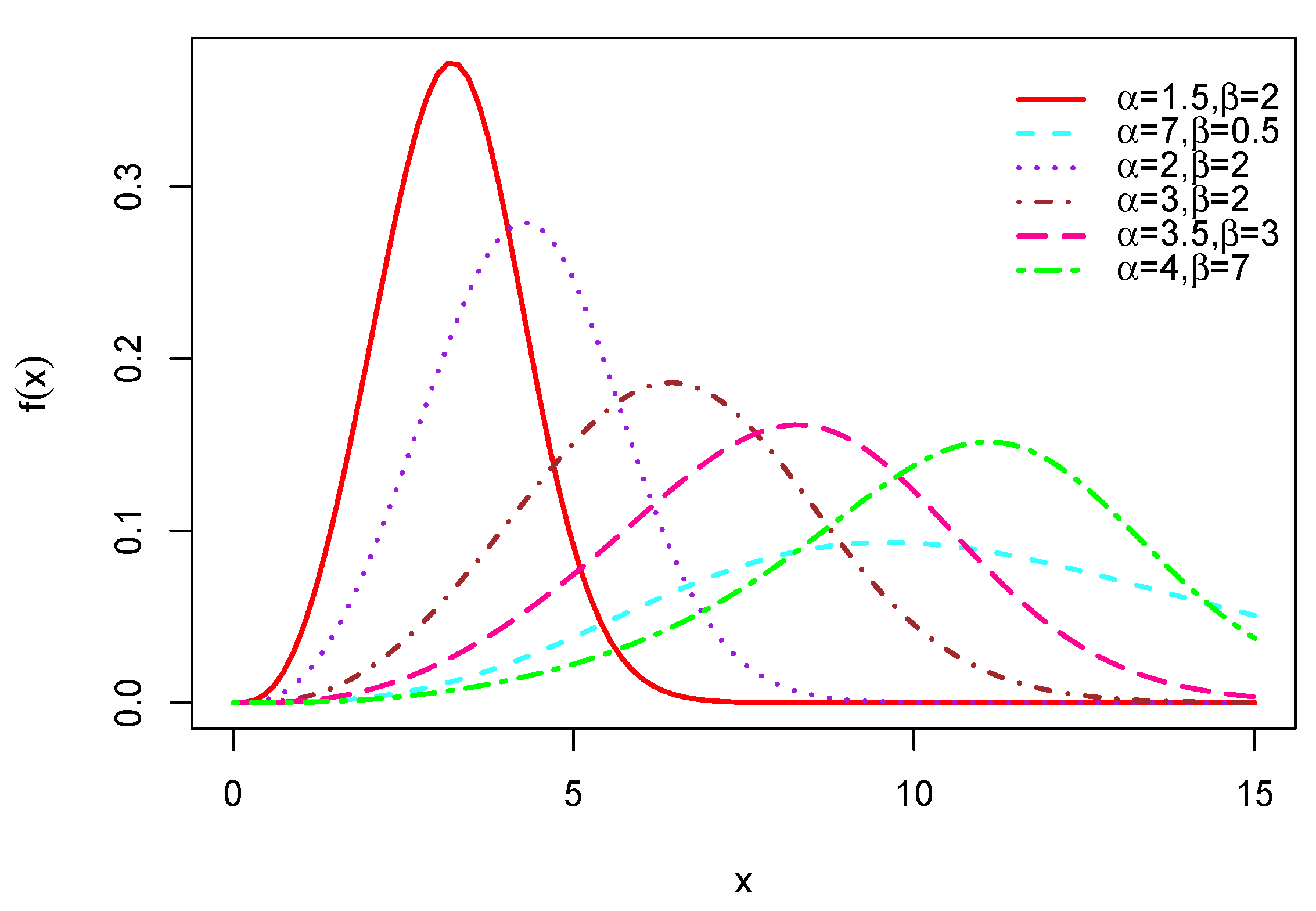
Based on (2), some analytical facts about $f_{MOLBM}(x;\alpha ,\beta )$ are now discussed. First, we have $f_{MOLBM}(0;\alpha ,\beta )=0$ with $f_{MOLBM}(x;\alpha ,\beta )\sim x^3/\left(2{\alpha }^4\beta \right)$ when $x\to 0$. In addition, we have $f_{MOLBM}(x;\alpha ,\beta )\to 0$ when $x\to +\infty$, along with the following equivalence: $f_{MOLBM}(x;\alpha ,\beta )\sim \beta x^3{e}^{-x^2/\left(2{\alpha }^2\right)}/\left(2{\alpha }^4\right)$. Hence, the convergence to 0 is with a polynomial-exponential decay. Let us now discuss the maximum(s) and possible shapes of $f_{MOLBM}(x;\alpha ,\beta )$ through a graphical analysis. In this aim, several curves of $f_{MOLBM}(x;\alpha ,\beta )$ are shown in Figure 1 for diverse values of $\alpha$ and $\beta$.

This figure shows that the pdf of the MOLBM distribution has many shape possibilities; it can be bell shaped, right-skewed, left-skewed with all types of peakedness and with various weights on the tails. These combined qualities are rare for a lifetime distribution.

2.3. Analysis of $h_{MOLBM}(x;\alpha ,\beta )$

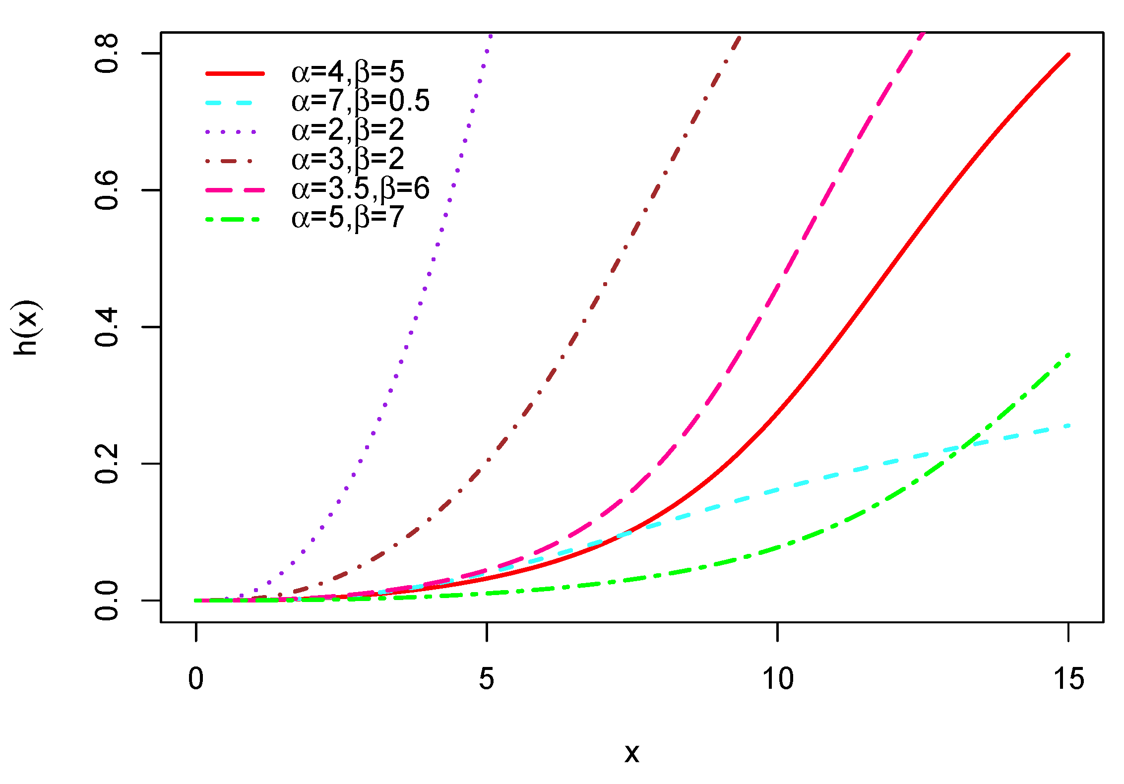
Here, we focus on $h_{MOLBM}(x;\alpha ,\beta )$. From (3), it is clear that $h_{MOLBM}(0;\alpha ,\beta )=0$, along with the following equivalence: $h_{MOLBM}(x;\alpha ,\beta )\sim x^3/\left(2{\alpha }^4\beta \right)$ when $x\to 0$. In addition, we have $h_{MOLBM}(x;\alpha ,\beta )\to +\infty$ when $x\to +\infty$, with $h_{MOLBM}(x;\alpha ,\beta )\sim x/{\alpha }^2$. Let us now investigate the mode and possible shapes of $h_{MOLBM}(x;\alpha ,\beta )$ through a graphical analysis. In this regard, several curves of $h_{MOLBM}(x;\alpha ,\beta )$ are displayed in Figure 2.

This figure shows that the hrf possesses increasing shapes, with concave and convex forms.

3. Compounding, Dominance and Moments

We now put the light on some interesting results involving the MOLBM distribution.

3.1. Compounding

The following theorem is about a compounding characterization of the MOLBM distribution.

Theorem 1.

Let X and Y be two random variables such that $X\mid \{Y=y\}$ has the following conditional sf:

$$S(x\mid y;\alpha )=exp\left\{-\left[e^{x^2/\left(2{\alpha }^2\right)}{\left(1+x^2/\left(2{\alpha }^2\right)\right)}^{-1}-1\right]y\right\},x>0$$

and $S(x\mid y;\alpha )=1$ for $x\le 0$, with $y>0$ and $\alpha >0$, and Y follows the exponential distribution with parameter $\beta >0$, i.e., with pdf $f_{Ex}(y;\beta )=\beta e^{-\beta y}$ for $y>0$ and $f_{Ex}(y;\beta )=0$ for $y\le 0$. Then, X follows the MOLBM distribution with parameters α and β.

Proof. 

By the definition, the sf of X is obtained as

$$\begin{array}{cc}\hfill S(x;\alpha ,\beta )& ={\int }_0^{+\infty }S(x\mid y;\alpha )f_{Ex}(y;\beta )dy\hfill \\ \hfill & =\beta {\int }_0^{+\infty }exp\left\{-\left[e^{x^2/\left(2{\alpha }^2\right)}{\left(1+x^2/\left(2{\alpha }^2\right)\right)}^{-1}-(1-\beta )\right]y\right\}dy\hfill \\ \hfill & =\beta {\int }_0^{+\infty }exp\left\{-\left[\frac{1-(1-\beta )e^{-x^2/\left(2{\alpha }^2\right)}\left(1+x^2/\left(2{\alpha }^2\right)\right)}{e^{-x^2/\left(2{\alpha }^2\right)}\left(1+x^2/\left(2{\alpha }^2\right)\right)}\right]y\right\}dy\hfill \\ \hfill & =\frac{\beta e^{-x^2/\left(2{\alpha }^2\right)}\left(1+x^2/\left(2{\alpha }^2\right)\right)}{1-(1-\beta )e^{-x^2/\left(2{\alpha }^2\right)}\left(1+x^2/\left(2{\alpha }^2\right)\right)}.\hfill \end{array}$$

We recognize $S_{MOLBM}(x;\alpha ,\beta )$, ending the proof of Theorem 1. □

3.2. Stochastic Dominance

The following first-order stochastic dominance result holds.

Proposition 1.

For any $0<{\alpha }_1\le {\alpha }_2$, $0\le {\beta }_1\le {\beta }_2$, and $x\in \mathbb{R}$, we have

$$F_{MOLBM}(x;{\alpha }_2,{\beta }_2)\le F_{MOLBM}(x;{\alpha }_1,{\beta }_1).$$

Proof. 

This inequality is clear for $x\le 0$, the both cdfs being equal to 0. For $x>0$, we have

$$\begin{array}{c}\hfill \frac{\partial }{\partial \alpha }{F}_{MOLBM}(x;\alpha ,\beta )=-\frac{2\beta x^4{e}^{x^2/\left(2{\alpha }^2\right)}}{\alpha {\left[2{\alpha }^2(e^{x^2/\left(2{\alpha }^2\right)}+\beta -1)+(\beta -1)x^2\right]}^2}<0\end{array}$$

and

$$\begin{array}{c}\hfill \frac{\partial }{\partial \beta }{F}_{MOLBM}(x;\alpha ,\beta )=-\frac{e^{-x^2/\left(2{\alpha }^2\right)}\left(1+x^2/\left(2{\alpha }^2\right)\right)\left[1-e^{-x^2/\left(2{\alpha }^2\right)}\left(1+x^2/\left(2{\alpha }^2\right)\right)\right]}{{\left[1-(1-\beta )e^{-x^2/\left(2{\alpha }^2\right)}\left(1+x^2/\left(2{\alpha }^2\right)\right)\right]}^2}<0.\end{array}$$

Therefore, $F_{MOLBM}(x;\alpha ,\beta )$ is a decreasing function with respect to $\alpha$ and $\beta$, proving the desired result. □

In particular, since $F_{MOLBM}(x;\alpha ,1)=F_{LBM}(x;\alpha )$, Proposition 1 implies the following first-order stochastic dominance related to the MOLBM and LBM distributions: For $\beta \in (0,1)$, we have $F_{LBM}(x;\alpha )\le F_{MOLBM}(x;\alpha ,\beta )$, and for $\beta \ge 1$, $F_{MOLBM}(x;\alpha ,\beta )\le F_{LBM}(x;\alpha )$.

The MOLBM distribution also enjoys a strong hazard rate dominance, formulated in the next result.

Proposition 2.

For any $0\le {\beta }_1\le {\beta }_2$ and $x\in \mathbb{R}$, we have

$$h_{MOLBM}(x;\alpha ,{\beta }_2)\le h_{MOLBM}(x;\alpha ,{\beta }_1).$$

Proof. 

This inequality is clear for $x\le 0$, the both hrfs being equal to 0. For $x>0$, we have

$$\begin{array}{c}\hfill \frac{\partial }{\partial \beta }{h}_{MOLBM}(x;\alpha ,\beta )=-\frac{x^3{e}^{-x^2/\left(2{\alpha }^2\right)}}{2{\alpha }^4{\left[1-(1-\beta )e^{-x^2/\left(2{\alpha }^2\right)}\left(1+x^2/\left(2{\alpha }^2\right)\right)\right]}^2}<0.\end{array}$$

Therefore, $h_{MOLBM}(x;\alpha ,\beta )$ is a decreasing function with respect to $\beta$, proving the desired result. □

In particular, since $h_{MOLBM}(x;\alpha ,1)$ corresponds to the hazard rate function of the LBM distribution denoted by $h_{LBM}(x;\alpha )$, the following hazard rate dominance result holds: For $\beta \in (0,1)$, we have $h_{LBM}(x;\alpha )\le h_{MOLBM}(x;\alpha ,\beta )$, and for $\beta \ge 1$, $h_{MOLBM}(x;\alpha ,\beta )\le h_{LBM}(x;\alpha )$.

All the above results demonstrate the power of $\beta$ in the pliancy of the MOLBM distribution in comparison to the classic LBM distribution. For further results about the first-order stochastic dominance, we refer the reader to [22].

3.3. Moments

Hereafter, we work with a random variable X following the MOLBM distribution with parameters $\alpha >0$ and $\beta >0$. Then, for any integer s, the $s^{\mathrm{th}}$ moment of X is obtained as

$$\begin{array}{c}\hfill {\theta }_s=\mathbb{E}\left(X^s\right)={\int }_0^{+\infty }{x}^s{f}_{MOLBM}(x;\alpha ,\beta )dx,\end{array}$$

where $\mathbb{E}$ denotes the expectation. Thanks to the obtained equivalences functions of $f_{MOLBM}(x;\alpha ,\beta )$ at $x\to 0$ and $x\to +\infty$, owing to the Riemann integral criteria, ${\theta }_s$ exists in the integral convergence sense.

However, in view of the complexity of $f_{MOLBM}(x;\alpha ,\beta )$, there is no simple analytical expression for ${\theta }_s$. From a computational point of view, numerical integration techniques can be employed to evaluate it through the use of mathematical software. A more transparency, direct and analytical approach consists in providing series expansion for ${\theta }_s$. A such expansion is given in the following result for the case $\beta \in (0,1)$ through the use of the gamma function defined by $\Gamma \left(a\right)={\int }_0^{+\infty }{t}^{a-1}{e}^{-t}dt$ with $a>0$.

Proposition 3.

For $\beta \in (0,1)$, we have

$$\begin{array}{cc}\hfill {\theta }_s& =\beta 2^{s/2}{\alpha }^s\sum _{k=0}^{+\infty }\sum _{\ell =0}^k\left(\genfrac{}{}{0pt}{}{k}{\ell }\right)\frac{{(1-\beta )}^k}{{(k+1)}^{s/2+\ell +1}}\Gamma \left(\frac{s}{2}+\ell +2\right).\hfill \end{array}$$

Proof. 

In the case $\beta \in (0,1)$, we have $(1-\beta )e^{-x^2/\left(2{\alpha }^2\right)}\left(1+x^2/\left(2{\alpha }^2\right)\right)\in (0,1)$. By applying the geometric series formula, followed by the classic binomial formula, a series expansion of $f_{MOLBM}(x;\alpha ,\beta )$ is given as

$$\begin{array}{cc}\hfill f_{MOLBM}(x;\alpha ,\beta )& =\frac{\beta x^3{e}^{-x^2/\left(2{\alpha }^2\right)}}{2{\alpha }^4}\left\{\sum _{k=0}^{+\infty }(k+1){(1-\beta )}^k{e}^{-k{x}^2/\left(2{\alpha }^2\right)}{\left(1+\frac{x^2}{2{\alpha }^2}\right)}^k\right\}\hfill \\ \hfill & =\frac{\beta x^3{e}^{-x^2/\left(2{\alpha }^2\right)}}{2{\alpha }^4}\left\{\sum _{k=0}^{+\infty }\sum _{\ell =0}^k\left(\genfrac{}{}{0pt}{}{k}{\ell }\right)(k+1){(1-\beta )}^k{e}^{-k{x}^2/\left(2{\alpha }^2\right)}\frac{x^{2\ell }}{{\left(2{\alpha }^2\right)}^{\ell }}\right\}\hfill \\ \hfill & =\sum _{k=0}^{+\infty }\sum _{\ell =0}^k{u}_{k,\ell }\left[x^{2\ell +3}{e}^{-(k+1)x^2/\left(2{\alpha }^2\right)}\right],u_{k,\ell }=\frac{\beta }{2^{\ell +1}{\alpha }^{2\ell +4}}\left(\genfrac{}{}{0pt}{}{k}{\ell }\right)(k+1){(1-\beta )}^k.\hfill \end{array}$$

Now, by the dominated convergence theorem, we get

$$\begin{array}{cc}\hfill {\theta }_s& =\sum _{k=0}^{+\infty }\sum _{\ell =0}^k{u}_{k,\ell }{{\rm Y}}_{k,\ell |s},{{\rm Y}}_{k,\ell |s}={\int }_0^{+\infty }{x}^{s+2\ell +3}{e}^{-(k+1)x^2/\left(2{\alpha }^2\right)}dx.\hfill \end{array}$$

By applying the change of variable $y=(k+1)x^2/\left(2{\alpha }^2\right)$ and introducing the well-known gamma function, we can express ${{\rm Y}}_{k,\ell |s}$ as

$$\begin{array}{c}\hfill {{\rm Y}}_{k,\ell |s}=\frac{2^{s/2+\ell +1}{\alpha }^{s+2\ell +4}}{{(k+1)}^{s/2+\ell +2}}{\int }_0^{+\infty }{y}^{s/2+\ell +1}{e}^{-y}dy=\frac{2^{s/2+\ell +1}{\alpha }^{s+2\ell +4}}{{(k+1)}^{s/2+\ell +2}}\Gamma \left(\frac{s}{2}+\ell +2\right).\end{array}$$

(5)

Therefore, by putting the previous equalities together, we get

$$\begin{array}{cc}\hfill {\theta }_s& =\beta 2^{s/2}{\alpha }^s\sum _{k=0}^{+\infty }\sum _{\ell =0}^k\left(\genfrac{}{}{0pt}{}{k}{\ell }\right)\frac{{(1-\beta )}^k}{{(k+1)}^{s/2+\ell +1}}\Gamma \left(\frac{s}{2}+\ell +2\right).\hfill \end{array}$$

This ends the proof of Proposition 3. □

From Proposition 3, it is clear that ${\theta }_s$ is an increasing function with respect to $\alpha$.

The case $\beta =1$, corresponding to the classic LBM distribution, can be found in [12]. From this reference, the following formula is reported:

$${\theta }_s=2^{s/2}{\alpha }^s\Gamma \left(\frac{s}{2}+2\right).$$

The next result discusses a series expansion for ${\theta }_s$ in the case $\beta >1$, demanding another strategy of proof.

Proposition 4.

For $\beta >1$, we have

$$\begin{array}{cc}\hfill {\theta }_s& =\frac{2^{s/2}{\alpha }^s}{\beta }\sum _{k=0}^{+\infty }\sum _{\ell =0}^k\sum _{m=0}^{\ell }\left(\genfrac{}{}{0pt}{}{k}{\ell }\right)\left(\genfrac{}{}{0pt}{}{\ell }{m}\right)(k+1)\frac{{\left(1-1/\beta \right)}^k{(-1)}^{\ell }}{{(\ell +1)}^{s/2+m+2}}\Gamma \left(\frac{s}{2}+m+2\right).\hfill \end{array}$$

Proof. 

In the case $\beta >1$, in view of using some generic formula, we need to re-express $f_{MOLBM}(x;\alpha ,\beta )$. In this regard, for $x>0$, we have

$$f_{MOLBM}(x;\alpha ,\beta )=\frac{x^3{e}^{-x^2/\left(2{\alpha }^2\right)}}{2{\alpha }^4\beta {\left\{1-(1-1/\beta )\left[1-e^{-x^2/\left(2{\alpha }^2\right)}\left(1+x^2/\left(2{\alpha }^2\right)\right)\right]\right\}}^2}.$$

Now, let us notice that $(1-1/\beta )\left[1-e^{-x^2/\left(2{\alpha }^2\right)}\left(1+x^2/\left(2{\alpha }^2\right)\right)\right]\in (0,1)$. By applying the geometric series formula, followed by the classic binomial formula two times in a row, the following series expansion of $f_{MOLBM}(x;\alpha ,\beta )$ holds:

$$\begin{array}{cc}\hfill & f_{MOLBM}(x;\alpha ,\beta )=\frac{x^3{e}^{-x^2/\left(2{\alpha }^2\right)}}{2{\alpha }^4\beta }\left\{\sum _{k=0}^{+\infty }(k+1){\left(1-\frac{1}{\beta }\right)}^k{\left[1-e^{-x^2/\left(2{\alpha }^2\right)}\left(1+\frac{x^2}{2{\alpha }^2}\right)\right]}^k\right\}\hfill \\ \hfill & =\frac{x^3{e}^{-x^2/\left(2{\alpha }^2\right)}}{2{\alpha }^4\beta }\left\{\sum _{k=0}^{+\infty }\sum _{\ell =0}^k\sum _{m=0}^{\ell }\left(\genfrac{}{}{0pt}{}{k}{\ell }\right)\left(\genfrac{}{}{0pt}{}{\ell }{m}\right)(k+1){\left(1-\frac{1}{\beta }\right)}^k{(-1)}^{\ell }{e}^{-\ell x^2/\left(2{\alpha }^2\right)}\frac{x^{2m}}{{\left(2{\alpha }^2\right)}^m}\right\}\hfill \\ \hfill & =\sum _{k=0}^{+\infty }\sum _{\ell =0}^k\sum _{m=0}^{\ell }{v}_{k,\ell ,m}\left[x^{2m+3}{e}^{-(\ell +1)x^2/\left(2{\alpha }^2\right)}\right],\hfill \end{array}$$

where

$$v_{k,\ell ,m}=\frac{1}{\beta 2^{m+1}{\alpha }^{2m+4}}\left(\genfrac{}{}{0pt}{}{k}{\ell }\right)\left(\genfrac{}{}{0pt}{}{\ell }{m}\right)(k+1){\left(1-\frac{1}{\beta }\right)}^k{(-1)}^{\ell }.$$

Now, by the dominated convergence theorem, we get

$$\begin{array}{cc}\hfill {\theta }_s& =\sum _{k=0}^{+\infty }\sum _{\ell =0}^k\sum _{m=0}^{\ell }{v}_{k,\ell ,m}{\Xi }_{\ell ,m|s},{\Xi }_{\ell ,m|s}={\int }_0^{+\infty }{x}^{s+2m+3}{e}^{-(\ell +1)x^2/\left(2{\alpha }^2\right)}dx.\hfill \end{array}$$

By proceeding as in (5), we arrive at

$${\Xi }_{\ell ,m|s}=\frac{2^{s/2+m+1}{\alpha }^{s+2m+4}}{{(\ell +1)}^{s/2+m+2}}{\int }_0^{+\infty }{y}^{s/2+m+1}{e}^{-y}dy=\frac{2^{s/2+m+1}{\alpha }^{s+2m+4}}{{(\ell +1)}^{s/2+m+2}}\Gamma \left(\frac{s}{2}+m+2\right).$$

Therefore, by putting the previous equalities together, we get

$$\begin{array}{cc}\hfill {\theta }_s& =\frac{2^{s/2}{\alpha }^s}{\beta }\sum _{k=0}^{+\infty }\sum _{\ell =0}^k\sum _{m=0}^{\ell }\left(\genfrac{}{}{0pt}{}{k}{\ell }\right)\left(\genfrac{}{}{0pt}{}{\ell }{m}\right)(k+1)\frac{{\left(1-1/\beta \right)}^k{(-1)}^{\ell }}{{(\ell +1)}^{s/2+m+2}}\Gamma \left(\frac{s}{2}+m+2\right).\hfill \end{array}$$

This ends the proof of Proposition 4. □

From Proposition 4, as for the case $\beta \in (0,1)$, we can notice ${\theta }_s$ is an increasing function with respect to $\alpha$. By combining Propositions 3 and 4, we can derive a manageable approximation finite sum expression of ${\theta }_s$ by substituting the infinite limits by large integers. From the computational point of view, such series approximation can be more precise than direct integral approximation techniques from the initial definition of ${\theta }_s$.

Remark 1.

One can show that $\mathbb{E}\left(X^{\upsilon }\right)$ exists provided $\upsilon >-4$, allowing the consideration of some negative moments for X. The $s^{\mathrm{th}}$ negative moment being defined by

$$\begin{array}{c}\hfill {\theta }_s^{-}=\mathbb{E}\left(X^{-s}\right)={\int }_0^{+\infty }{x}^{-s}{f}_{MOLBM}(x;\alpha ,\beta )dx.\end{array}$$

Therefore, for $s=1$, 2 and 3, ${\theta }_s^{-}$ can be expressed as ${\theta }_s$ in Propositions 3 and 4 by putting $-s$ instead of s in the series expansions.

The moments of X include the mean of X corresponding to ${\theta }_1$. The variance of X is obtained by the standard Koenig–Huygens formula: $V={\theta }_2-{\theta }_1^2$. In addition, the $s^{\mathrm{th}}$ central moment of X is obtained as

$$\begin{array}{cc}\hfill {\theta }_s^o& =\mathbb{E}\left({(X-{\theta }_1)}^s\right)=\sum _{\ell =0}^s\left(\genfrac{}{}{0pt}{}{s}{\ell }\right){(-1)}^{s-\ell }{\theta }_1^{s-\ell }{\theta }_{\ell }.\hfill \end{array}$$

From this central moment, we can define the $s^{\mathrm{th}}$ general coefficient of X by $G_s={\theta }_s^o/V^{s/2}$. The coefficients of asymmetry and kurtosis of X are given as $G_3$ and $G_4$, respectively.

Table 1. Numerical values for moments, asymmetry and kurtosis of the MOLBM distribution for selected values of the parameters.

$(\mathit{\alpha },\mathit{\beta })$	${\mathit{\theta }}_1$ (${\mathit{\theta }}_1^{-})$	${\mathit{\theta }}_2$(${\mathit{\theta }}_2^{-})$	${\mathit{\theta }}_3$ (${\mathit{\theta }}_3^{-})$	${\mathit{\theta }}_4$	V	${\mathit{G}}_3$	${\mathit{G}}_4$
$(0.005,100)$	0.0184	0.0008	1.01$\times {10}^{-6}$	1.3$\times {10}^{-8}$	0.0005	$-2.9011$	5.0819
	(57.1350)	(4528.16)	(274,453)
$(0.05,20)$	0.1524	0.0243	0.0039	0.0006	0.0010	$-1.6821$	27.7787
	(7.0120)	(55.3985)	(598.8584)
$(75,25)$	234.5479	57,449.4207	14,572,745	3,783,926,248	2436.636	$-0.3737$	$-0.7699$
	(0.0045)	(0.00002)	(1.5$\times {10}^{-7}$)
$(0.5,2)$	1.0757	1.2802	1.6493	2.2691	0.1230	0.1693	2.9014
	(1.0693)	(1.4253)	(2.9580)
$(15,0.5)$	14.1882	311.9162	8183.9644	246,252	110.6081	0.5327	3.0209
	(0.0765)	(0.0008)	(0.0001)
$(20,0.05)$	5.9051	126.1360	3444.8536	115,297	91.2657	1.8604	6.8036
	(0.0389)	(0.0020)	(0.0004)
$(100,0.005)$	7.0709	532.4942	57,231.6903	8,346,402.62	482.4955	4.4009	29.5526
	(0.0047)	(0.00001)	(9.4183$\times {10}^{-7}$)

indicates numerical values for moments (standard and negative), asymmetry and kurtosis of the MOLBM distribution for selected values of parameters $\alpha$ and $\beta$.

From this table, we see wide variations in the values of the mean, the other moments and negatives moments. The variance can be small or large. In addition, the MOLBM distribution can have $G_3<0$ or $G_3>0$, revealing the versatile nature of its skewness. The same remark holds for the kurtosis; we have $G_4<3$, $G_4\approx 3$ or $G_4>3$, showing that the MOLBM distribution can be platykurtic, mesokurtic or leptokurtic, respectively.

3.4. Incomplete Moments

Let $t\ge 0$ and $I(X\le t)$ be the indicator random variable over the event $\{X\le t\}$, that is $I(X\le t)=1$ if $\{X\le t\}$ realized, and 0 otherwise. Then, for any integer s, the $s^{\mathrm{th}}$ incomplete moment of X at t exists and it is obtained as

$$\begin{array}{c}\hfill {\theta }_s\left(t\right)=\mathbb{E}\left(X^{s}I(X\le t)\right)={\int }_0^t{x}^s{f}_{MOLBM}(x;\alpha ,\beta )dx.\end{array}$$

An analytical expression for ${\theta }_s\left(t\right)$ is not expected, but numerical integration techniques can be considered. Alternatively, we can express it as in Propositions 3 and 4 through the use of the lower incomplete gamma function defined by $\gamma (a,x)={\int }_0^x{t}^{a-1}{e}^{-t}dt$ with $a>0$ and $t\ge 0$. The proposition below formalizes this expression, according to $\beta \in (0,1)$, $\beta =1$ and $\beta >1$.

Proposition 5.

The following expansions for ${\theta }_s\left(t\right)$ hold:

• For $\beta \in (0,1)$, we have

  $$\begin{array}{cc}\hfill {\theta }_s\left(t\right)& =\beta 2^{s/2}{\alpha }^s\sum _{k=0}^{+\infty }\sum _{\ell =0}^k\left(\genfrac{}{}{0pt}{}{k}{\ell }\right)\frac{{(1-\beta )}^k}{{(k+1)}^{s/2+\ell +1}}\gamma \left(\frac{s}{2}+\ell +2,\frac{k+1}{2{\alpha }^2}{t}^2\right).\hfill \end{array}$$
• For $\beta =1$, we have

  $$\begin{array}{cc}\hfill {\theta }_s\left(t\right)& =2^{s/2}{\alpha }^s\gamma \left(\frac{s}{2}+2,\frac{t^2}{2{\alpha }^2}\right).\hfill \end{array}$$
• For $\beta >1$, we have

  $$\begin{array}{cc}\hfill {\theta }_s\left(t\right)& =\frac{2^{s/2}{\alpha }^s}{\beta }\sum _{k=0}^{+\infty }\sum _{\ell =0}^k\sum _{m=0}^{\ell }\left(\genfrac{}{}{0pt}{}{k}{\ell }\right)\left(\genfrac{}{}{0pt}{}{\ell }{m}\right)(k+1)\frac{{\left(1-1/\beta \right)}^k{(-1)}^{\ell }}{{(\ell +1)}^{s/2+m+2}}\gamma \left(\frac{s}{2}+m+2,\frac{\ell +1}{2{\alpha }^2}{t}^2\right).\hfill \end{array}$$

The proof of Proposition 5 follows the lines of Propositions 3 and 4, just an adjustment of the upper bound in the integral needs special treatment according to the respective changes of variables. For this reason, the detailed proof is omitted.

By applying $t\to +\infty$, we rediscover the $s^{\mathrm{th}}$ moment of X. Several related quantities can be derived from $m_s\left(t\right)$, such as the mean deviation about the mean defined by

$$\delta =\mathbb{E}\left(\right|X-{\theta }_1\left|\right)={\int }_0^{+\infty }|x-{\theta }_1|f_{MOLBM}(x;\alpha ,\beta )dx=2{\theta }_1{F}_{MOLBM}({\theta }_1;\alpha ,\beta )-2{\theta }_1\left({\theta }_1\right),$$

where ${\theta }_1\left({\theta }_1\right)$ denotes the first incomplete moment of X taken at $t={\theta }_1$. As a second famous example, one can discuss the reversed residual life of X defined by

$${\mathsf{\Phi }}_s\left(t\right)=\mathbb{E}\left({(t-X)}^{s}I(X\le t)\right)=\frac{1}{F_{MOLBM}(t;\alpha ,\beta )}{\int }_0^t{(t-x)}^s{f}_{MOLBM}(x;\alpha ,\beta )dx,$$

where, by the classic binomial formula, the integral term can be developed as

$$\begin{array}{cc}\hfill {\int }_0^t{(t-x)}^s{f}_{MOLBM}(x;\alpha ,\beta )dx& =\sum _{k=0}^s\left(\genfrac{}{}{0pt}{}{s}{k}\right)t^{s-k}{(-1)}^k{\theta }_k\left(t\right).\hfill \end{array}$$

We thus have a generic expression for ${\mathsf{\Phi }}_s\left(t\right)$ according to the incomplete moments, from which we can deduce the mean waiting time of X by taking $s=1$. Similarly, the variance and coefficient of variation of the reversed residual life of X can be defined from ${\mathsf{\Phi }}_1\left(t\right)$ and ${\mathsf{\Phi }}_2\left(t\right)$. More details are provided in [23].

4. Estimation

In view of exploring the fitting behavior of the MOLBM model, we discuss the estimation of the parameters via the famous maximum likelihood method.

4.1. Estimates

Let $x_1,\dots ,x_n$ be n values distributed from the MOLBM distribution with parameters $\alpha >0$ and $\beta >0$. We now assume that $\alpha$ and $\beta$ are unknown, and seek to estimate them via $x_1,\dots ,x_n$. In this regard, the maximum likelihood approach is considered. The likelihood function of $\alpha$ and $\beta$ based on $x_1,\dots ,x_n$ is given by

$$\begin{array}{cc}\hfill L(\alpha ,\beta )& =\prod _{i=1}^n{f}_{MOLBM}(x_i;\alpha ,\beta )\hfill \\ \hfill & =\frac{{\beta }^n\left({\prod }_{i=1}^n{x}_i^3\right)e^{-[1/\left(2{\alpha }^2\right)]{\sum }_{i=1}^n{x}_i^2}}{2^n{\alpha }^{4n}{\prod }_{i=1}^n{\left[1-(1-\beta )e^{-x_i^2/\left(2{\alpha }^2\right)}\left(1+x_i^2/\left(2{\alpha }^2\right)\right)\right]}^2},\hfill \end{array}$$

from which we deduce the log-likelihood function obtained as

$$\begin{array}{cc}\hfill \ell (\alpha ,\beta )& =nlog\beta -nlog2-4nlog\alpha +3\sum _{i=1}^{n}log{x}_i-\frac{1}{2{\alpha }^2}\sum _{i=1}^n{x}_i^2\hfill \\ \hfill & -2\sum _{i=1}^{n}log\left[1-(1-\beta )e^{-x_i^2/\left(2{\alpha }^2\right)}\left(1+\frac{x_i^2}{2{\alpha }^2}\right)\right].\hfill \end{array}$$

The maximum likelihood estimates (MLEs) of $\alpha$ and $\beta$ are defined by

$$(\widehat{\alpha },\widehat{\beta })={argmax}_{(\alpha ,\beta )\in {(0,+\infty )}^2}\ell (\alpha ,\beta ),$$

assuming that there are uniques. That is, $\widehat{\alpha }$ and $\widehat{\beta }$ satisfy the score equations corresponding to $\partial \ell (\alpha ,\beta )/\partial \alpha {\mid }_{\alpha =\widehat{\alpha },\beta =\widehat{\beta }}=0$, that is

$$\begin{array}{c}\hfill {\left.-\frac{4n}{\alpha }+\frac{1}{{\alpha }^3}\sum _{i=1}^n{x}_i^2-\frac{\beta -1}{{\alpha }^5}\sum _{i=1}^n\frac{x_i^4{e}^{-x_i^2/\left(2{\alpha }^2\right)}}{1-(1-\beta )e^{-x_i^2/\left(2{\alpha }^2\right)}\left(1+x_i^2/\left(2{\alpha }^2\right)\right)}\right|}_{\alpha =\widehat{\alpha },\beta =\widehat{\beta }}=0,\end{array}$$

and $\partial \ell (\alpha ,\beta )/\partial \beta {\mid }_{\alpha =\widehat{\alpha },\beta =\widehat{\beta }}=0$, that is

$$\begin{array}{cc}\hfill & {\left.\frac{n}{\beta }-2\sum _{i=1}^n\frac{e^{-x_i^2/\left(2{\alpha }^2\right)}\left(1+x_i^2/\left(2{\alpha }^2\right)\right)}{1-(1-\beta )e^{-x_i^2/\left(2{\alpha }^2\right)}\left(1+x_i^2/\left(2{\alpha }^2\right)\right)}\right|}_{\alpha =\widehat{\alpha },\beta =\widehat{\beta }}=0.\hfill \end{array}$$

The mathematical expressions of $\widehat{\alpha }$ and $\widehat{\beta }$ depending $x_1,\dots ,x_n$ are not available. However, their numerical values can be determined via statistical softwares. Theoretical results guarantee the convergence of the MLEs in several senses, including the following desirable asymptotic normality. Under some smoothness conditions, we have $(\widehat{\alpha },\widehat{\beta })\sim {\mathcal{N}}_2((\alpha ,\beta ),C)$, where

$$C={\left(\begin{array}{cc}{c}_{1,1}(\alpha ,\beta )& c_{1,2}(\alpha ,\beta )\\ c_{2,1}(\alpha ,\beta )& c_{2,2}(\alpha ,\beta )\end{array}\right)}^{-1},$$

$$c_{1,1}(\alpha ,\beta )=-\frac{{\partial }^2}{\partial {\alpha }^2}\ell (\alpha ,\beta ),c_{2,2}(\alpha ,\beta )=-\frac{{\partial }^2}{\partial {\beta }^2}\ell (\alpha ,\beta ),c_{1,2}(\alpha ,\beta )=c_{2,1}(\alpha ,\beta )=-\frac{{\partial }^2}{\partial \alpha \partial \beta }\ell (\alpha ,\beta ).$$

From this result, the estimated standard errors (SEs) corresponding to $\widehat{\alpha }$ and $\widehat{\beta }$ are, respectively, given as

$${\mathrm{SE}}_{\widehat{\alpha }}={\left.\sqrt{\frac{c_{2,2}(\alpha ,\beta )}{\Delta (\alpha ,\beta )}}\right|}_{\alpha =\widehat{\alpha },\beta =\widehat{\beta }},{\mathrm{SE}}_{\widehat{\beta }}={\left.\sqrt{\frac{c_{1,1}(\alpha ,\beta )}{\Delta (\alpha ,\beta )}}\right|}_{\alpha =\widehat{\alpha },\beta =\widehat{\beta }},$$

where $\Delta (\alpha ,\beta )=c_{2,2}(\alpha ,\beta )c_{1,1}(\alpha ,\beta )-c_{1,2}{(\alpha ,\beta )}^2$. In addition, the maximum likelihood approach allows us to define some criteria to compare the fit behavior of different models, such as the AIC, CAIC, BIC and HQIC. In the case of the MOLBM model, they are defined by

$$\begin{array}{cc}\hfill & \mathrm{AIC}=-2logL+2k,\mathrm{CAIC}=-2logL+\frac{2kn}{n-k-1},\hfill \\ \hfill & \mathrm{BIC}=-2logL+klog\left(n\right),\mathrm{HQIC}=-2logL+2klog(log(n\left)\right),\hfill \end{array}$$

where $-logL=-\ell (\widehat{\alpha },\widehat{\beta })$ and $k=2$ is the number of parameters. In the simulated and concrete applications of this study, R will be used (see [24]).

4.2. Simulation

A Monte Carlo simulation study is conducted for the MOLBM model. The results are obtained from 1000 Monte Carlo replications and the simulations are carried out using the statistical software R. In each replication, a random sample of size 10, 20, 30, 50 and 100 is generated for different combinations of $\alpha$ and $\beta$. The combination values of $\alpha$ and $\beta$ are $(0.75,0.4)$, $(0.75,1.5)$, $(0.5,0.5)$, $(0.5,1.5)$ and $(1.2,0.5)$.

Table 2. Estimates, biases and mean squared errors (MSEs) for $\alpha =0.75$ and $\beta =0.4$.

Sample Size (n)	Parameters	Estimates	Biases	MSEs
10	$\alpha$	0.1975	$-0.5524$	0.4492
	$\beta$	0.5397	0.1397	4.5310
20	$\alpha$	0.2779	$-0.4720$	0.4652
	$\beta$	0.3733	$-0.0266$	0.8851
30	$\alpha$	0.3938	$-0.3561$	0.3993
	$\beta$	0.3730	$-0.0269$	0.4443
50	$\alpha$	0.5864	$-0.1635$	0.3541
	$\beta$	0.4278	0.0278	0.2246
100	$\alpha$	0.6157	$-0.1342$	0.1341
	$\beta$	0.4081	0.0081	0.0979

,

Table 3. Estimates, biases and MSEs for $\alpha =0.75$ and $\beta =1.5$.

Sample Size (n)	Parameters	Estimates	Biases	MSEs
10	$\alpha$	0.7360	$-0.0139$	0.1338
	$\beta$	7.1195	5.6195	433.1667
20	$\alpha$	0.7461	$-0.0038$	0.1172
	$\beta$	3.0168	1.5168	15.3585
30	$\alpha$	0.7532	0.0032	0.0758
	$\beta$	2.3176	0.8176	5.6637
50	$\alpha$	0.7472	$-0.0027$	0.0070
	$\beta$	1.9418	0.4418	1.9821
100	$\alpha$	0.7489	$-0.001$0	0.0032
	$\beta$	1.6727	0.1727	0.5373

,

Table 4. Estimates, biases and MSEs for $\alpha =0.5$ and $\beta =0.5$.

Sample Size (n)	Parameters	Estimates	Biases	MSEs
10	$\alpha$	0.1231	$-0.3768$	0.2132
	$\beta$	0.9647	0.4647	49.7625
20	$\alpha$	0.4079	$-0.0920$	0.2659
	$\beta$	0.9165	0.4165	6.2857
30	$\alpha$	0.5026	0.0026	0.0735
	$\beta$	0.9406	0.4406	1.1700
50	$\alpha$	0.5025	0.0025	0.0376
	$\beta$	0.7437	0.2437	0.3841
100	$\alpha$	0.4987	$-0.0012$	0.0035
	$\beta$	0.5992	0.0992	0.1135

,

Table 5. Estimates, biases and MSEs for $\alpha =0.5$ and $\beta =1.5$.

Sample Size (n)	Parameters	Estimates	Biases	MSEs
10	$\alpha$	0.4840	$-0.01597$	0.0325
	$\beta$	6.3054	4.8054	385.5095
20	$\alpha$	0.4975	$-0.0024$	0.0408
	$\beta$	2.9662	1.4662	13.2258
30	$\alpha$	0.4987	$-0.0012$	0.0230
	$\beta$	2.3570	0.8570	5.2564
50	$\alpha$	0.4988	$-0.0011$	0.0033
	$\beta$	1.9295	0.4295	1.6671
100	$\alpha$	0.4994	$-0.0005$	0.0014
	$\beta$	1.6842	0.1842	0.5081

and

Table 6. Estimates, biases and MSEs for $\alpha =1.2$ and $\beta =0.5$.

Sample Size (n)	Parameters	Estimates	Biases	MSEs
10	$\alpha$	0.4919	$-0.7080$	1.3195
	$\beta$	0.9573	0.4573	11.3779
20	$\alpha$	1.2441	0.0441	0.9715
	$\beta$	1.1786	0.6786	2.3047
30	$\alpha$	1.2325	0.0325	0.6709
	$\beta$	0.9305	0.4305	0.9875
50	$\alpha$	1.2264	0.0264	0.3633
	$\beta$	0.7026	0.2026	0.3233
100	$\alpha$	1.2112	0.0112	0.0644
	$\beta$	0.5868	0.0868	0.1046

list the average MLEs, biases and the corresponding mean squared errors (MSEs).

The results in these tables reveal that the estimates are stable and relatively close to the true parameter values for these sample sizes. In particular, as expected, the MSEs decrease as n increases from 20.

5. Applications

In this section, we explore the potentiality of the new model with other five well known competitive models which are the Marshall–Olkin length-biased exponential (MOLBE), Marshall–Olkin extended Lindley (MOEL) (see [25]), generalized Rayleigh (GR) (see [26]), Weibull and length-biased Maxwell (LBM) models. For the sake of transparency, the pdfs of these competitive models are expressed below.

The pdf of the MOLBE model is

$$\begin{array}{c}\hfill f_{MOLBE}(x;\alpha ,\beta )=\frac{\alpha x{e}^{-x/\beta }}{{\beta }^2{\left[1-(1-\alpha )(1+x/\beta )e^{-x/\beta }\right]}^2},x>0,\end{array}$$

and $f_{MOLBE}(x;\alpha ,\beta )=0$ for $x\le 0$.

The pdf of the MOEL model is

$$\begin{array}{c}\hfill f_{MOEL}(x;\alpha ,\beta )=\frac{\alpha {\beta }^2(1+x)e^{-\beta x}}{(\beta +1){\left[1-(1-\alpha )(1+\beta x/(\beta +1))e^{-\beta x}\right]}^2},x>0,\end{array}$$

and $f_{MOEL}(x;\alpha ,\beta )=0$ for $x\le 0$.

The pdf of the GR model is

$$\begin{array}{c}\hfill f_{GR}(x;\alpha ,\beta )=2\alpha {\beta }^{2}x{e}^{-{\left(\beta x\right)}^2}{\left(1-e^{-{\left(\beta x\right)}^2}\right)}^{\alpha -1},x>0,\end{array}$$

and $f_{GR}(x;\alpha ,\beta )=0$ for $x\le 0$.

The pdf of the Weibull model is

$$\begin{array}{c}\hfill f_{Weibull}(x;\alpha ,\beta )=\frac{\beta }{\alpha }{\left(\frac{x}{\alpha }\right)}^{\beta -1}{e}^{-{(x/\alpha )}^{\beta }},x>0,\end{array}$$

and $f_{Weibull}(x;\alpha ,\beta )=0$ for $x\le 0$.

The pdf of the LBM model is

$$\begin{array}{c}\hfill f_{LBM}(x;\alpha )=\frac{1}{2{\alpha }^4}{x}^3{e}^{-x^2/\left(2{\alpha }^2\right)},x>0,\end{array}$$

and $f_{LBM}(x;\alpha )=0$ for $x\le 0$.

All the involved parameters $\alpha$ and $\beta$ are supposed to be strictly positive.

The five data sets considered are given below, along with the estimated model parameters, the values of the following models comparison criteria: AIC, CAIC, BIC and HQIC, and the following goodness-of-fit statistics values: $A^{*}$, $W^{*}$ and KS, as well as the p-value of the KS test. We recall that a lower AIC, BIC, CAIC, BIC, HQIC, $A^{*}$, $W^{*}$ or KS value indicates a better fit for the corresponding model. Moreover, the larger the p-value of the KS test, the less we can reject the suitability of the model to fit the data.

Data set 1: The data are extracted from [27]. They represent the failure times of mechanical components. They are given as follows: 30.94, 18.51, 16.62, 51.56, 22.85, 22.38, 19.08, 49.56, 17.12, 10.67, 25.43, 10.24, 27.47, 14.70, 14.10, 29.93, 27.98, 36.02, 19.40, 14.97, 22.57, 12.26, 18.14, 18.84.

Table 7. Estimates and standard errors (in parentheses) of the parameters for Data set 1.

Models	$\mathit{\alpha }$	$\mathit{\beta }$
MOLBM	21.5256 (11.4235)	0.0849 (0.1721)
MOLBE	9.7838 (8.0270)	5.3859 (1.1659)
MOEL	12.0423 (9.9529)	0.1885 (0.0393)
GR	1.6630 (0.5149)	0.0463 (0.0057)
Weibull	26.0260 (2.4458)	2.3091 (0.3377)
LBM	12.6351 (0.9118)	-

shows the MLEs of the parameters of the considered models, with their standard errors.

Table 8. Some criteria and goodness of fit measures for Data set 1.

Model	−$log\mathit{L}$	AIC	CAIC	BIC	HQIC	${\mathit{A}}^{*}$	${\mathit{W}}^{*}$	KS	p-Value
MOLBM	86.2493	176.4986	177.0700	178.8547	177.1237	0.2184	0.0278	0.0991	0.9538
MOLBE	88.8814	181.7629	182.3343	184.1190	182.3880	0.6057	0.0694	0.1257	0.7982
MOEL	89.0309	182.0618	182.6332	184.4179	182.6869	0.6197	0.0699	0.1274	0.7852
GR	88.0440	180.0882	180.6596	182.4443	180.7133	0.6661	0.1014	0.1660	0.4723
Weibull	88.8909	181.7820	182.3532	184.1381	182.4069	0.7470	0.1083	0.1437	0.6523
LBM	88.9802	179.9605	180.1423	181.1386	180.2730	1.1852	0.1940	0.2120	0.2001

indicates the −$logL$, AIC, CAIC, BIC, HQIC, $A^{*}$, $W^{*}$, KS and p-value of the considered models.

A global conclusion on the fit behavior of the MOLBM model for the five data sets will be formulated later.

Data set 2: The data are taken from [28]. They represent fracture toughness MPa $m^{1/2}$ data from the Alumina $\left(A{l}_2{O}_3\right)$ material. They are given as follows: 5.5, 5, 4.9, 6.4, 5.1, 5.2, 5.2, 5, 4.7, 4, 4.5, 4.2, 4.1, 4.56, 5.01, 4.7, 3.13, 3.12, 2.68, 2.77, 2.7, 2.36, 4.38, 5.73, 4.35, 6.81, 1.91, 2.66, 2.61, 1.68, 2.04, 2.08, 2.13, 3.8, 3.73, 3.71, 3.28, 3.9, 4, 3.8, 4.1, 3.9, 4.05, 4, 3.95, 4, 4.5, 4.5, 4.2, 4.55, 4.65, 4.1, 4.25, 4.3, 4.5, 4.7, 5.15, 4.3, 4.5, 4.9, 5, 5.35, 5.15, 5.25, 5.8, 5.85, 5.9, 5.75, 6.25, 6.05, 5.9, 3.6, 4.1, 4.5, 5.3, 4.85, 5.3, 5.45, 5.1, 5.3, 5.2, 5.3, 5.25, 4.75, 4.5, 4.2, 4, 4.15, 4.25, 4.3, 3.75, 3.95, 3.51, 4.13, 5.4, 5, 2.1, 4.6, 3.2, 2.5, 4.1, 3.5, 3.2, 3.3, 4.6, 4.3, 4.3, 4.5, 5.5, 4.6, 4.9, 4.3, 3, 3.4, 3.7, 4.4, 4.9, 4.9, 5.

Table 9. Estimates and standard errors (in parentheses) of the parameters for Data set 2.

Model	$\mathit{\alpha }$	$\mathit{\beta }$
MOLBM	1.4870 (0.0649)	14.0943 (5.3469)
MOLBE	568.6299 (330.1662)	0.5089 (0.0364)
MOEL	1208.9799 (742.3799)	1.9306 (0.1382)
GR	4.9728 (0.7871)	0.3370 (0.0139)
Weibull	4.7131 (0.0914)	4.9649 (0.3562)
LBM	2.2213 (0.0719)	-

shows the MLEs of the parameters of the considered models, with their standard errors.

Table 10. Some criteria and goodness of fit measures for Data set 2.

Model	−$log\mathit{L}$	AIC	CAIC	BIC	HQIC	${\mathit{A}}^{*}$	${\mathit{W}}^{*}$	KS	p-Value
MOLBM	167.6899	339.3799	339.4832	344.9381	341.6368	0.2935	0.0424	0.0482	0.9445
MOLBE	170.0202	344.0405	344.1438	349.5987	346.2974	0.5320	0.0573	0.0530	0.8918
MOEL	170.1588	344.3176	344.4210	349.8759	346.5746	0.5478	0.0586	0.0534	0.8860
GR	176.9805	357.9610	358.0644	363.5193	360.2180	2.3203	0.3972	0.1285	0.0391
Weibull	168.7069	341.4137	341.5172	346.9720	343.6708	0.5431	0.0839	0.0720	0.5665
LBM	189.1835	380.3669	380.4012	383.1460	381.4955	7.0059	1.3320	0.2037	0.0001

indicates the −$logL$, AIC, CAIC, BIC, HQIC, $A^{*}$, $W^{*}$, KS and p-value of the considered models.

Data set 3: The data are taken from [29]. These data represent the monthly taxes revenue in Egypt. They are given as follows: 5.9, 20.4, 14.9, 16.2, 17.2, 7.8, 6.1, 9.2, 10.2, 9.6, 13.3, 8.5, 21.6, 18.5, 5.1, 6.7, 17, 8.6, 9.7, 39.2, 35.7, 15.7, 9.7, 10, 4.1, 36, 8.5, 8, 9.2, 26.2, 21.9, 16.7, 21.3, 35.4, 14.3, 8.5, 10.6, 19.1, 20.5, 7.1, 7.7, 18.1, 16.5, 11.9, 7, 8.6, 12.5, 10.3, 11.2, 6.1, 8.4, 11, 11.6, 11.9, 5.2, 6.8, 8.9, 7.1, 10.8.

Table 11. Estimates and standard errors (in parentheses) of the parameters for Data set 3.

Model	$\mathit{\alpha }$	$\mathit{\beta }$
MOLBM	15.4189 (4.0534)	0.0308 (0.0314)
MOLBE	2.5119 (1.3294)	4.7696 (0.9069)
MOEL	3.5707 (1.8257)	0.2221 (0.0380)
GR	1.0310 (0.1844)	0.0644 (0.0056)
Weibull	15.3060 (1.1511)	1.8406 (0.1711)
LBM	7.8367 (0.3607)	-

shows the MLEs of the parameters of the considered models, with their standard errors.

Table 12. Some criteria and goodness of fit measures for Data set 3.

Model	−$log\mathit{L}$	AIC	CAIC	BIC	HQIC	${\mathit{A}}^{*}$	${\mathit{W}}^{*}$	KS	p-Value
MOLBM	190.5571	385.1141	385.3285	389.2692	386.7362	0.9461	0.1326	0.0994	0.6044
MOLBE	196.8304	397.6609	397.8751	401.8159	399.2828	1.6284	0.2241	0.1261	0.3050
MOEL	198.1121	400.2241	400.4385	404.3792	401.8462	1.7622	0.2402	0.1302	0.2696
GR	197.6964	399.3927	399.6071	403.5478	401.0148	2.2879	0.3971	0.1764	0.0507
Weibull	197.2905	398.5811	398.7953	402.7361	400.2030	1.8404	0.2803	0.1431	0.1778
LBM	209.4001	420.8002	420.8704	422.8777	421.6112	9.3091	1.5012	0.2898	0.0000

indicates the −$logL$, AIC, CAIC, BIC, HQIC, $A^{*}$, $W^{*}$, KS and p-value of the considered models.

Data set 4: The data are taken from [30]. They represent the strengths of 1.5 cm glass fibers. They are given as follows: 0.55, 0.74, 0.77, 0.81, 0.84, 1.24, 0.93, 1.04, 1.11, 1.13, 1.30, 1.25, 1.27, 1.28, 1.29, 1.48, 1.36, 1.39, 1.42, 1.48, 1.51, 1.49, 1.49, 1.50, 1.50, 1.55, 1.52, 1.53, 1.54, 1.55, 1.61, 1.58, 1.59, 1.60, 1.61, 1.63, 1.61, 1.61, 1.62, 1.62, 1.67, 1.64, 1.66, 1.66, 1.66, 1.70, 1.68, 1.68, 1.69, 1.70, 1.78, 1.73, 1.76, 1.76, 1.77, 1.89, 1.81, 1.82, 1.84, 1.84, 2.00, 2.01, 2.24.

Table 13. Estimates and standard errors (in parentheses) of the parameters for Data set 4.

Model	$\mathit{\alpha }$	$\mathit{\beta }$
MOLBM	0.4646 (0.0253)	39.4015 (23.2301)
MOLBE	1977.1222 (1.8 × ${10}^3$)	0.1544 (1.5× ${10}^{-2}$)
MOEL	6400.3238 (6682.1222)	6.2326 (0.6538)
GR	5.4848 (1.1848)	0.9868 (0.0539)
Weibull	1.6281 (0.0371)	5.7793 (0.5759)
LBM	0.7703 (0.0343)	-

shows the MLEs of the parameters of the considered models, with their standard errors.

Table 14. Some criteria and goodness of fit measures for Data set 4.

Model	−$log\mathit{L}$	AIC	CAIC	BIC	HQIC	${\mathit{A}}^{*}$	${\mathit{W}}^{*}$	KS	p-Value
MOLBM	12.6613	29.3226	29.5226	33.6089	31.0084	0.7307	0.1023	0.1052	0.4873
MOLBE	15.5968	35.1936	35.3936	39.4799	36.8794	1.2144	0.1653	0.1235	0.2912
MOEL	15.8503	35.7006	35.9006	39.9869	37.3864	1.2587	0.1699	0.1247	0.2810
GR	23.9287	51.8575	52.0575	56.1437	53.5433	3.1284	0.5829	0.2150	0.0059
Weibull	15.2068	34.4136	34.6136	38.6999	36.0994	1.2412	0.2152	0.1522	0.1077
LBM	31.9066	65.8133	65.8789	67.9565	66.6562	6.1291	1.2265	0.2648	0.0002

indicates the −$logL$, AIC, CAIC, BIC, HQIC, $A^{*}$, $W^{*}$, KS and p-value of the considered models.

Data set 5: The data are taken from [31]. These data represent the survival times of injected guinea pigs with different doses of tubercle bacilli. They are given as follows: 34, 38, 38, 43, 44, 48, 52, 53, 54, 54, 55, 56, 57, 58, 58, 59, 60, 60, 60, 60, 61, 62, 63, 65, 65, 67, 68, 70, 70, 72, 73, 75, 76, 76, 81, 83, 84, 85, 87, 91, 95, 96, 98, 99, 109, 110, 121, 127, 129, 131, 143, 146, 175, 175, 211, 233, 258, 258, 263, 297, 341, 341, 376.

Table 15. Estimates and standard errors (in parentheses) of the parameters for Data set 5.

Model	$\mathit{\alpha }$	$\mathit{\beta }$
MOLBM	142.5637 (27.6842)	0.0119 (0.0090)
MOLBE	0.5478 (0.3876)	70.2665 (23.7620)
MOEL	0.5837 (0.3842)	0.0144 (0.0044)
GR	0.7176 (0.1162)	0.0065 (0.0006)
Weibull	122.1597 (10.7737)	1.5217 (0.1358)
LBM	67.7747 (3.0177)	-

gives the MLEs of the parameters of the considered models, with their standard errors.

Table 16. Some criteria and goodness of fit measures for Data set 5.

Model	−$log\mathit{L}$	AIC	CAIC	BIC	HQIC	${\mathit{A}}^{*}$	${\mathit{W}}^{*}$	KS	p-Value
MOLBM	340.3010	684.6020	684.8020	688.8883	686.2878	2.6973	0.2383	0.1213	0.3117
MOLBE	346.1912	696.3824	696.5824	700.6687	698.0682	3.0670	0.5144	0.1766	0.0391
MOEL	346.6147	697.2294	697.4294	701.5157	698.9152	3.1350	0.5310	0.1753	0.0416
GR	352.9955	709.9909	710.1910	714.2772	711.6768	5.2559	1.0402	0.2381	0.0015
Weibull	349.7034	703.4067	703.6068	707.6930	705.0926	3.7094	0.6570	0.1821	0.0306
LBM	383.9953	769.9905	770.0562	772.1336	770.8335	27.4030	4.0878	0.4192	0.0000

presents the −$logL$, AIC, CAIC, BIC, HQIC, $A^{*}$, $W^{*}$, KS and p-value of the considered models.

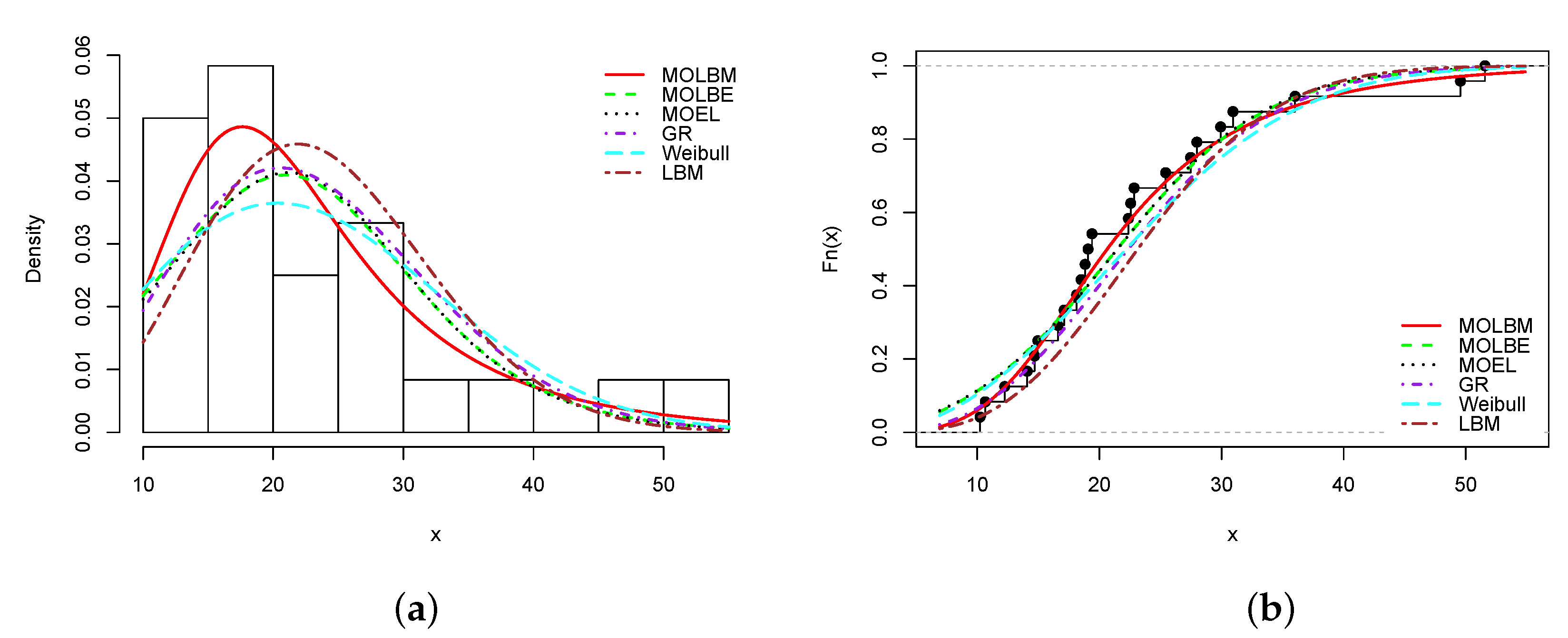
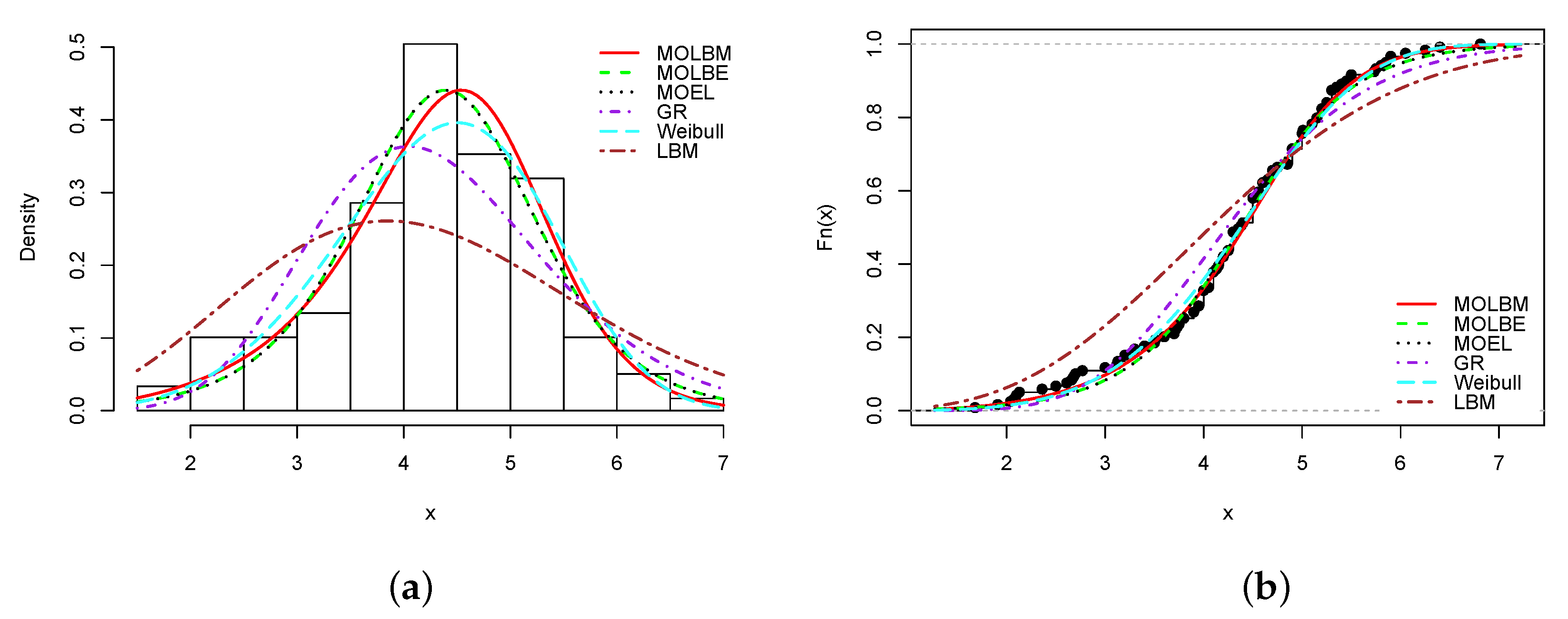
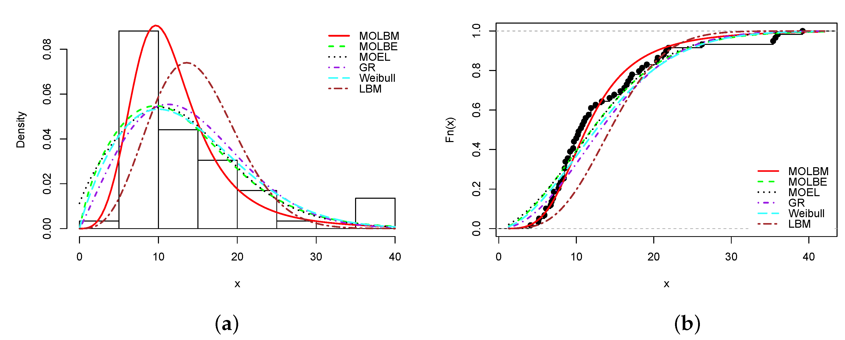
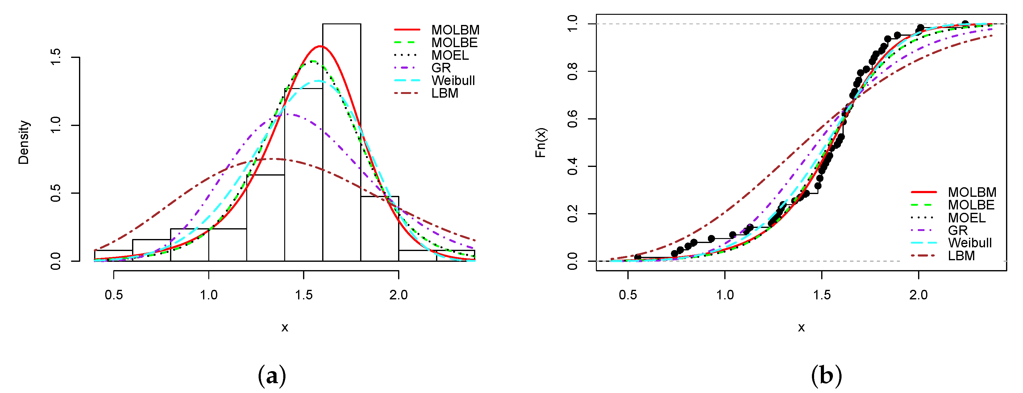
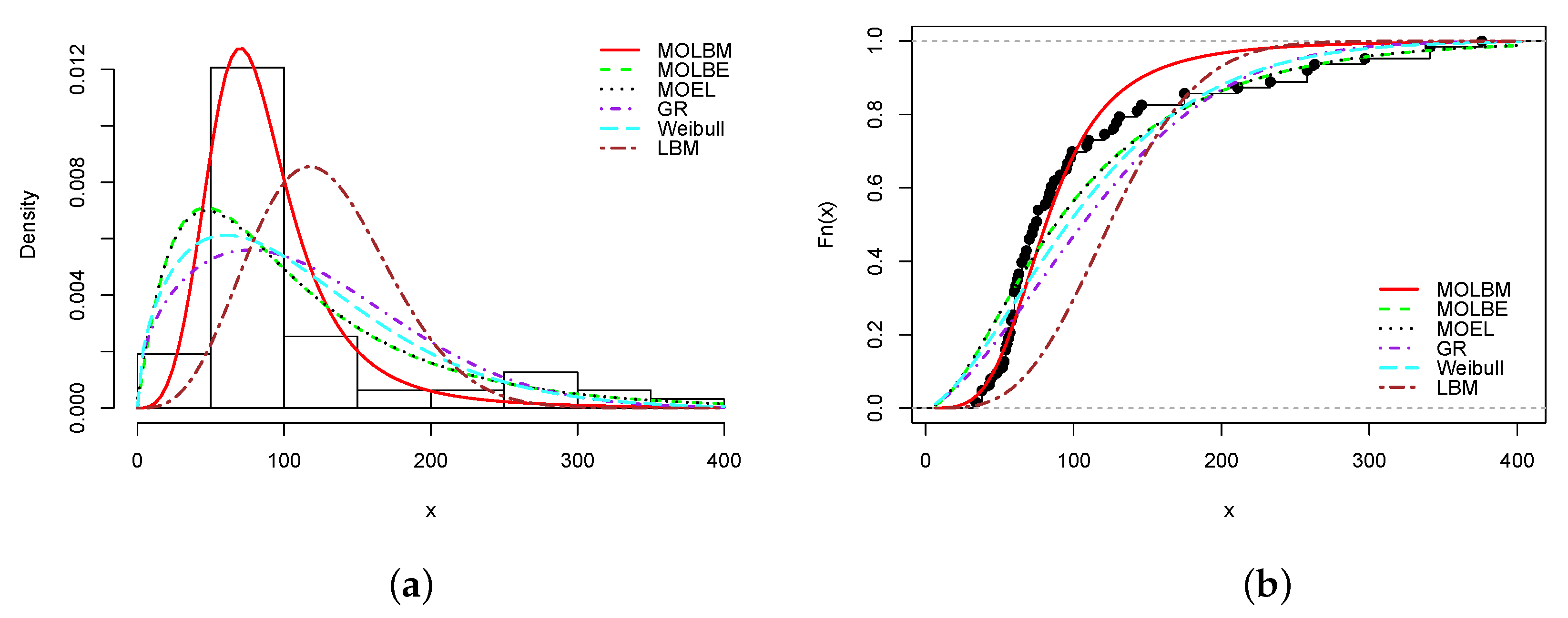
From Table 8, Table 10, Table 12, Table 14 and Table 16, it is clear that the smallest AIC, CAIC, BIC, HQIC, $A^{*}$, $W^{*}$ and KS statistics, and largest KS p-value are obtained for the MOLBM model; it is the best model. As the main illustrations, the plots of the estimated pdfs over the histograms and cdfs over the empirical cdfs are presented in Figure 3, Figure 4, Figure 5, Figure 6 and Figure 7 for Data sets 1, 2, 3, 4 and 5, respectively.

In all the graphs, we see that the red curves fit the empirical objects better than the other colored curves. From these numerical and visual evidences, we can conclude that the MOLBM model can be adequate for modeling these data.

6. Conclusion with Perspectives

In this article, we introduced a generalization of the length-biased Maxwell distribution known as Marshall–Olkin length-biased Maxwell distribution. We studied its statistical properties such as compounding, stochastic dominance, moments and incomplete moments in detail. In addition, we estimated the parameter of the distribution via maximum likelihood estimation method and checked the stability of the parameters using a Monte Carlo simulation study. Five referenced data sets are used to check the flexibility of the new model and found a better fit than the other five well known competitive models, namely the Marshall–Olkin length-biased exponential, Marshall–Olkin extended Lindley, generalized Rayleigh, Weibull and length-biased Maxwell models. The success of this new model motivates greater possibilities and future prospects. One of these possibilities is discussed below. First, we can notice that the cdfs of the length-biased exponential and length-biased Maxwell distributions can be written in the following form:

$$\begin{array}{c}\hfill F(x;\tau ,m,\upsilon )=1-e^{-x^{\tau }/\upsilon }\sum _{k=0}^m\frac{{(x^{\tau }/\upsilon )}^k}{k!},x>0,\end{array}$$

(6)

and $F(x;\tau ,m,\upsilon )=0$ for $x\le 0$, where $\tau >0$, m denotes a positive integer and $\upsilon >0$. This function is a valid cdf; it corresponds to the cdf of a power version of the Erlang distribution. Thus, a possible direction of work can be the study of the Marshall–Olkin transformation of (6) in the general case, or under a “new motivated and simple” configuration for $\tau$ and m to reduce the complexity, like in Marshall–Olkin length-biased exponential and Marshall–Olkin length-biased Maxwell distributions.

References

- Tyagi, R.K.; Bhattacharya, S.K. A note on the MVU estimation of reliability for the Maxwell failure distribution. Estadistica 1989, 41, 73–79. [Google Scholar]
- Chaturvedi, A.; Rani, U. Classical and Bayesian reliability estimation of the generalized Maxwell failure distribution. J. Stat. Res. 1998, 32, 113–120. [Google Scholar]
- Bekker, A.; Roux, J.J. Reliability characteristics of the Maxwell distribution: A Bayes estimation study. Commun. Stat. Theory Methods 2005, 34, 2169–2178. [Google Scholar] [CrossRef]
- Kazmi, S.M.A.; Aslam, M.; Sajid, A. A note on the maximum likelihood estimators for the mixture of Maxwell distributions using type-I censored scheme. Open Stat. Probab. J. 2011, 3, 31–35. [Google Scholar] [CrossRef] [Green Version]
- Kazmi, S.M.A.; Aslam, M.; Sajid, A. Preference of prior for the class of lifetime distributions under different loss functions. Pak. J. Stat. 2012, 28, 467–484. [Google Scholar]
- Radha, R.K.; Venkatesan, P. On the double prior selection for the parameter of Maxwell distribution. Int. J. Sci. Eng. Res. 2013, 4, 1238–1241. [Google Scholar]
- Tomer, S.K.; Panwar, M.S. Estimation procedures for Maxwell distribution under type I progressive hybrid censoring scheme. J. Stat. Comput. Simul. 2015, 85, 339–356. [Google Scholar] [CrossRef]
- Arslan, T.; Acitas, S.; Senoglu, B. Parameter estimation for the two-parameter Maxwell distribution under complete and censored samples. Revstat 2017, 1, 1–20. [Google Scholar]
- Venegas, O.; Iriarte, Y.; Astorga, J.M.; Börger, A.; Bolfarine, H.; Gómez, H.W. A new generalization of the Maxwell distribution. Appl. Math. Inf. Sci. 2017, 11, 867–876. [Google Scholar] [CrossRef]
- Sarma, S.; Das, K.K. A new one parameter Rayleigh Maxwell distribution. J. Math. Comput. Sci. 2020, 10, 1948–1959. [Google Scholar]
- Modi, K.; Gill, V. Length-biased weighted Maxwell distribution. Pak. J. Stat. Oper. Res. 2015, 11, 465–472. [Google Scholar] [CrossRef] [Green Version]
- Saghir, A.; Khadim, A.; Lin, Z. The Maxwell length-biased distribution: Properties and estimation. J. Stat. Theory Pract. 2017, 11, 26–40. [Google Scholar] [CrossRef]
- Saghir, A.; Khadim, A. The mathematical properties of length biased Maxwell distribution. J. Basic Appl. Res. Int. 2016, 16, 189–195. [Google Scholar]
- Saghir, A.; Hamedani, G.G.; Tazeem, S.; Khadim, A. Weighted distributions: A brief review, perspective and characterizations. Int. J. Stat. Probab. 2017, 6, 109–131. [Google Scholar] [CrossRef] [Green Version]
- Lindley, D.V. Fiducial distributions and Bayes theorem. J. R. Stat. Soc. A 1958, 20, 102–107. [Google Scholar] [CrossRef]
- Shanker, R. Shanker distribution and its applications. Int. J. Stat. Appl. 2015, 5, 338–348. [Google Scholar] [CrossRef] [Green Version]
- Dara, S.T.; Ahmad, M. Recent Advances in Moment Distribution and Their Hazard Rates; Lap Lambert Academic Publishing: Riga, Latvia, 2012. [Google Scholar]
- Ramos, P.L.; Louzada, F. A distribution for instantaneous failures. Stats 2019, 2, 19. [Google Scholar] [CrossRef] [Green Version]
- Haq, M.A.; Usman, R.M.; Hashmi, S.; Al-Omeri, A.I. The Marshall–Olkin length-biased exponential distribution and its applications. J. King Saud Univ. Sci. 2017, 4763, 1–11. [Google Scholar] [CrossRef]
- Marshall, A.W.; Olkin, I. A new method for adding a parameter to a family of distributions with application to the exponential and Weibull families. Biometrica 1997, 84, 641–652. [Google Scholar] [CrossRef]
- Aarset, M.V. How to identify bathtub hazard rate. IEEE Trans. Reliab. 1987, 36, 106–108. [Google Scholar] [CrossRef]
- Shaked, M.; Shanthikumar, J.G. Stochastic Orders; Wiley: New York, NY, USA, 2007. [Google Scholar]
- Barlow, R.E.; Proschan, F. Statistical Theory of Reliability and Life Testing; Holt, Rinehart, and Winston: New York, NY, USA, 1975. [Google Scholar]
- R Development Core Team. R: A language and environment for statistical computing. Available online: http://www.R-project.org (accessed on 30 September 2020).
- Ghitany, M.E.; Al-Mutairi, D.K.; Al-Awadhi, F.A.; Al-Burais, M.M. Marshall–Olkin extended Lindley distribution and its application. Int. J. Appl. Math. 2012, 25, 709–721. [Google Scholar]
- Kundu, D.; Raqab, M.Z. Generalized Rayleigh distribution: Different methods of estimations. Comput. Stat. Data Anal. 2005, 49, 187–200. [Google Scholar] [CrossRef]
- Murthy, D.P.; Xie, M.; Jiang, R. Weibull Models; John Wiley and Sons: Hoboken, NJ, USA, 2004; Volume 505. [Google Scholar]
- Ali, A.; Hasnain, S.A.; Ahmad, M. Modified Burr III distribution:Properties and Applications. Pak. J. Stat. 2015, 31, 697–708. [Google Scholar]
- Hassan, A.S.; Assar, S.M. The exponentiated Weibull power function distribution. J. Data Sci. 2017, 16, 589–614. [Google Scholar]
- Alzaatreh, A.; Ghosh, I. On the Weibull-X family of distributions. J. Stat. Theory Appl. 2015, 14, 169–183. [Google Scholar] [CrossRef] [Green Version]
- Bjerkedal, T. Acquisition of resistance in guinea pies infected with different doses of virulent tubercle bacilli. Am. J. Hyg. 1960, 72, 130–148. [Google Scholar] [PubMed]
Figure 1.
Curves of the pdf of the Marshall–Olkin length-biased Maxwell (MOLBM) distribution for different values of the parameters.
Figure 2.
Curves of the hrf of the MOLBM distribution for different values of the parameters.
Figure 3.
Plots of (a) estimated probability density function (pdf) and (b) estimated cumulative distribution function (cdf) of the MOLBM model with those of the other competitive models for Data set 1.
Figure 4.
Plots of (a) estimated pdf and (b) estimated cdf of the MOLBM model with those of the other competitive models for Data set 2.
Figure 5.
Plots of (a) estimated pdf and (b) estimated cdf of the MOLBM model with those of the other competitive models for Data set 3.
Figure 6.
Plots of (a) estimated pdf and (b) estimated cdf of the MOLBM model with those of the other competitive models for Data set 4.
Figure 7.
Plots of (a) estimated pdf and (b) estimated cdf of the MOLBM model with those of the other competitive models for Data set 5.