Convolutional Neural Network Based Ensemble Approach for Homoglyph Recognition

Abstract

Homoglyphs are pairs of visual representations of Unicode characters that look similar to the human eye. Identifying homoglyphs is extremely useful for building a strong defence mechanism against many phishing and spoofing attacks, ID imitation, profanity abusing, etc. Although there is a list of discovered homoglyphs published by Unicode consortium, regular expansion of Unicode character scripts necessitates a robust and reliable algorithm that is capable of identifying all possible new homoglyphs. In this article, we first show that shallow Convolutional Neural Networks are capable of identifying homoglyphs. We propose two variations, both of which obtain very high accuracy ($99.44\%$) on our benchmark dataset. We also report that adoption of transfer learning allows for another model to achieve 100% recall on our dataset. We ensemble these three methods to obtain 99.72% accuracy on our independent test dataset. These results illustrate the superiority of our ensembled model in detecting homoglyphs and suggest that our model can be used to detect new homoglyphs when increasing Unicode characters are added. As a by-product, we also prepare a benchmark dataset based on the currently available list of homoglyphs.

1. Introduction

With the Internet’s boom in the recent decades, the threat of losing invaluable personal and security information is growing exponentially. There is almost no end to virtual threats lurking in the shadow of the Internet waiting to pounce in moments of a user’s inattentiveness. One of many ways to realize such threats is to take advantage of the so-called homoglyphs, i.e., a pair of characters (that may be from the same or different alphabets) that are visually similar after being rendered by fonts [1,2]. For instance, Latin ‘a’ (U+0061) and Cyrillic ‘a’ (U+0430) look visually similar and they are almost impossible for human eyes to distinguish.

Homoglyphs are quite common in Unicode and, hence, could be exploited by an attacker. Being unaware that this might be a trap, she may click a link (containing the visually similar characters), or may do some other action that will lead to some unexpected and unwanted consequences. This article aims to explore how such homoglyphs can be discovered. The motivation behind this research principally comes from network security and related areas thereof. In particular, as has already been mentioned above, homoglyphs can be exploited to orchestrate a number of security threats, such as phishing attack, profanity abuse, ID imitation, etc., as briefly discussed below.

A phishing attack entraps an average user into submitting her personal (e.g., credit card number) or important security information (e.g., password) by presenting her with a link to a website that looks almost similar or even identical to a legitimate URL link or (a reputable) website. Additionally, mail clients who use Simple Mail Transfer Protocol (SMTP) may all be vulnerable to phishing emails.

Homoglyphs can also be exploited in bypassing profanity filters. Setting up an effective profanity filter is extremely important in the public (open) sites, especially those targeted to children or teenagers, because it is imperative to maintain decency therein by filtering out violent, indecent, or age-inappropriate words [3,4]. If the filter relies on hard-coded blacklisted words, a ‘predator’ can potentially and easily bypass that by replacing a letter of an abusive word with the help of homoglyphs [5]. Homoglyphs can also be cleverly exploited to impersonate another user’s ID in a social media and harm her reputation [6]. A person with malicious intent can open up an ID that looks similar to the popular ID, fool people, and sell them fake information, or harm them in some other way using the popularity and trust on that particular ID [7,8].

Identifying all known homoglyphs can be instrumental in developing a preventive defense mechanism against the attacks mentioned above. Identifying homoglyphs can reduce ID imitation instances using single script spoofing (to be discussed shortly) to a great extent. String matching algorithms combined with homoglyph-based character replacements can strengthen profanity filters. Recognizing all common homoglyphs between two different scripts can defend against whole script spoofing attacks (elaborated in Section 2) to a great extent. The main contributions of this paper can be summarized as follows (Codes for this research work can be found at: https://github.com/Taksir/Homoglyph).

• For the purpose of training and testing our models, we prepare a benchmark dataset based on already discovered homoglyphs (Section 4.1).
• We develop two shallow Convolutional Neural Networks (CNNs), namely ${CNN|}_{Scratch}^1$ and ${CNN|}_{Scratch}^2$, utilizing small filters to obtain very strong performance in the detection of homoglyphs (Section 5.1 and Section 5.2).
• We unfold how transfer learning with fine-tuning can also be utilized in order to develop a strong homoglyph detector despite the dissimilarity between the source and the target domains (in the context of transfer learning). In what follows, we will refer to this model as ${CNN|}_{Xfer}$ (Section 5.3).
• We describe how ensembling the above models’ strengths can be exploited to implement a final model that performs even better (Section 5.4).
• We achieve 98.83%, 98.61%, and 96% validation accuracy with ${CNN|}_{Scratch}^1$, ${CNN|}_{Scratch}^2$ and ${CNN|}_{Xfer}$, respectively. Our final ensemble model manages to achieve 99.72% accuracy in the test dataset. We compare the final ensemble model’s performance with state-of-the-art techniques and show that our model performs the best for detecting homoglyphs (Section 5.5).

2. Background

In this section, we briefly describe some background information.

2.1. Different Types of Spoofing

There are several types of Unicode based spoofing attacks [9,10]. Spoofing with characters entirely within one script is called single-script spoofing. Characters familiar across scripts (such as numbers) can be exploited in this attack category. In the whole script spoofing, a subset of characters of one script looking similar to a subset of characters of another is exploited, and that of the latter replaces all the characters of the former. For instance, the address http://apple.com, which is in Latin, can be phished by replacing all of the characters with characters from the Cyrillic alphabet, rendering visually identical output. On the other hand, in mixed-script spoofing, one or several characters are replaced while using other scripts. For example, the address http://spoofing.com may have one ‘o’ from Cyrillic and another ‘o’ from Omicron. Another type of spoofing is known as numeric spoofing, where visually similar digits or numbers from across different scripts are exploited. For instance, the English numeric digit of eight is identical to the Bangla numeric digit of four.

2.2. Convolutional Neural Network (CNN)

CNN [11] is a variation of deep neural networks that is mainly used in computer vision. Because we exploit CNNs in our models, here we give a very brief introduction thereof. CNN is the go-to deep learning architecture for most of the two-dimensional (2-D) image or vision-related problems. CNNs display computational efficiency as compared to normal feed-forward networks due to sharing of parameters and using fewer connections. The core part of CNN contributes convolutional layers that utilize convolution as a mathematical operation to merge two sets of information. The convolution is applied on the input data while using a convolution filter, which is slid over the input (it may be an image, or any other signal). The convolution operation consists of element-wise matrix multiplication and aggregation. Thus, feature maps are formed representing different features (low-level features in earlier layers and high-level features in the latter ones). Convolutional filters can be of size $3\times 3$, $5\times 5$, or more. Additionally, it is important to note that CNNs are capable of extracting relevant features on their own, thereby eliminating the need for manual feature engineering.

2.3. Transfer Learning

Transfer learning [12] refers to the technique that leverages knowledge that is gained from a previous similar task to a new task at hand. This is especially useful when supervised learning of a new task from a new domain suffers due to the lack of labelled training and test data. Transfer learning allows for the exploitation of data from a similar domain.

Convolutional neural networks usually learn low level features, such as edges and colors, in earlier layers. The mid level layers learn to detect comparatively higher level features such as geometric shapes. The high level layers generally learn high level features that are specific to the task at hand. Notably, in our case, color is negligible as a feature, since all of our images have the Unicode characters as black, and the background as white. However, Unicode characters can be thought of as an accumulation of many linear and non-linear edges. Hence, we can leverage low level features, including edges from another model and transfer the learning in our domain.

3. Related Works

Optical Character Recognition (OCR) techniques were the cornerstones of the earlier efforts for homoglyph detection. The main idea was to input character glyphs into OCR algorithms and observe whether they were incorrectly identified as other glyphs. The incorrectly mismatched character glyphs are considered to be homoglyphs [13]. The history of OCR techniques dates back to 1982 [14]. The works in [15,16,17,18,19,20] propose various OCR based methodologies in an attempt to recognise typewritten and handwritten text containing characters from many scripts. In some cases, OCR methods for typewritten text target one character glyph at a time. In other cases, they target one word at a time. The authors in [16] propose a Recurrent Neural Network based approach for word level segmentation. The authors in [19] propose two new feature descriptors, called Co-HOG and ConvCo-HOG, in order to detect scene characters of different languages.

The problem with applying OCR techniques for identifying homoglyphs is manifold. Firstly, it requires existing OCR techniques to recognise all possible Unicode characters. Secondly, it allows for us to find only one homoglyph for a particular glyph as input, whereas the other possible homoglyphs remain undiscovered. Thirdly, it does not take into account the fonts used and the performance metrics of the OCR techniques themselves. Last but not the least, they cannot handle working with new glyphs. Only the character glyphs present in the training data can reliably be tested against. This is a serious issue, as Unicode character sets are regularly expanding.

The work in [10] directly focuses on our problem and tries to find visually similar glyphs with the help of Kolmogorov complexity theory [21]. The intuition here is based on the fact that, if an image can not be described with respect to another image in any way at all, they are supposed to have a totally random relationship and be completely opposite to one another. Therefore, from the opposite angle, if a pair of glyphs have too much similarity, which is, less randomness than a certain threshold value, then they can be thought of as homoglyphs. Therefore, the authors in [10] compute normalized compression distance (NCD) to approximate the non-computable normalized information distance. They use the NCD function to measure the degree of similarity between two glyphs. Similar to our work, they also experiment with a subset of all Unicode characters. They exclude the ancient scripts and include 40 modern scripts, symbols, and punctuations (around 6200 characters) in their experiments. They argue that fixing a NCD value for measuring the similarity between two glyphs (so that they may be called homoglyphs) is a hard task, since it can depend on people’s perspective: what may seem as a homoglyph pair to one, may seem as a dissimilar pair to another. They experimented with different NCD values as a threshold and finally chose 0.25 as the best threshold value. since it generated around 5902 most probable pairs as homoglyphs. Their work has a serious limitation in the sense that the NCD value has to be tuned and agreed upon by lots of users. Notably, this work is also limited by available fonts.

Recently, Woodbridge et al. [22] have studied homoglyph based attacks and proposed a Siamese Convolutional Neural Network based approach to detect potential attacks. Their goal is not to detect homoglyphs directly. Instead, they extract feature vectors of URL strings as images and then index those features with randomized KD-trees in order to search for potential risky URLs that can be exploited for carrying out homoglyph based spoofing attacks. Effectively, the purpose of their work is to determine whether two URLs, rendered as images, look visually similar.

Koch et al. [23] exploited the Siamese Convolutional Neural Network earlier to distinguish between an image pair based on their class identity. Although their main purpose was one-shot image classification, their model could be used to evaluate images in a pairwise manner in order to determine whether they belong to the same class. As a result, their method can be used for training a model that can check whether two glyphs look similar.

Fu et al. [24] built a Unicode character similarity list based on the amount of visual semantic similarity between all pairs of characters. In order to measure character similarity, they used a nondeterministic finite automaton (NFA). Fu et al. ran a pixel-overlapping method to build a pattern generator to identify potential phishing patterns. Their work requires setting up a semantic similarity threshold value (that may vary from person to person). Moreover, they only used a single font in their experiment.

There exist a number of methods in the literature for image similarity detection, albeit not in the context of homoglyphs recognition directly. The Structural Similarity Index (SSIM) [25] is used for measuring similarity of two images. The Scale-Invariant Feature Transformation (SIFT) algorithm [26] can be applied to create image descriptors for two images, which can then be used for computing image similarity. Both of these methods can be used for calculating a similarity score. Additionally, Earth Mover’s Distance (EMD) can be used for obtaining a similarity score between two images, as reported in [27]. All of these methods may be exploited for building machine learning models in order to detect homoglyphs.

In the literature, several works exist that rely on the similarity between phishing sites and victim sites to establish a solid phishing detection mechanism. Liu et al. [28] proposed a block level, layout, and style based metric evaluation scheme for visual similarity detection. Fu et al. in [29] utilized earth mover’s distance (EMD) for visual similarity assessment. Similarly, [30,31] relied on manual feature extraction for visual similarity detection.

During the publication process of this manuscript, some more works have appeared in the literature. For example, Vinayakumar et al. in [32] proposed a Siamese CNN based network to detect visually similar domain names and compares them against approaches, such as edit distance and visual edit distance methods. Additionally, Lu et al., in [33], proposed a CNN network to detect domain name similarities. Unlike our character-based approach, this one is word-based and, hence, likely to face challenge when single characters are transformed.

4. Methodology

The Unicode Consortium published a list [34] of 6167 pairs of visually confusable characters. Most of these character pairs have been discovered and proposed as homoglyphs by several industry experts. Using these pairs of characters as the ground truth, we make an attempt to build up a machine learning model that can identify visually confusable characters. Such a model is expected to be useful for the professionals as (when) more character code points are being (will be) added to Unicode (in the future).

One can propose using manual feature extraction and applying template matching in order to identify a visually similar character pair. However, one attractive benefit of recently popular deep learning methods is that they can extract important features on their own [35]. CNNs can take pixels of images as input, learn features using its hidden layers and finally classify using the extracted feature information [36,37]. CNNs have repeatedly demonstrated their superiority over manual feature engineering of images by breaking their benchmarks [11,38,39,40]. Their powerful capability of extracting important features and removing noises on their own motivated us to utilize them for similarity detection in character pairs (all of which are similar in their own unique way).

We model and study this problem as a binary classification problem. Using the ground truth of the available confusable list, we feed the images of the pairs to a CNN model so that it can learn homoglyphs. However, we also need to teach it how to identify visually dissimilar looking pairs. Because this model needs to distinguish between a visually similar character pair and a visually dissimilar character pair, it can be thought of as a strong approximator for binary classification of images [41]. In other words, our CNN model will have to be a discriminative classifier that is based on similarity features that it would learn by itself during the training phase.

4.1. Dataset Generation

We omit Private Use Area (PUA) characters from the list of confusable character pairs provided by the Unicode consortium, since they are not defined by the Unicode consortium standard and are rather left to third parties for glyph formation, font creation etc. Also, we had difficulty in finding many of the fonts capable of rendering many scripts correctly. The work by [10] also faced similar problems during the dataset generation. Hence, the character pairs that were dependent on those fonts were also omitted in favor of having a cleaner dataset. Throughout the paper, we will refer to the set that consists of the character image pairs that look similar (dissimilar) as a similar (dissimilar) dataset. We used five fonts in total, namely, GNU, Unifont, EversonMono, Quivira, and Cunieform. For our similar dataset, we have 2257 character pairs. We have picked 1693 out of 2257 character pairs for the training, 385 character pairs for validation, and 179 character pairs for independent testing. For a binary classification problem, we need data with the opposite label, which, in this case, constitutes the different dataset. We have intentionally created a balanced dataset for our binary classification problem in order to avoid any issue related to imbalanced data [42,43]. The ratio of training-validation-test dataset is thus 75:17:8 (

Table 1. A short summary of the dataset.

Dataset	Similar Pairs	Dissimilar Pairs	Total Pairs
Training	1693	1693	3386
Validation	385	385	770
Test	179	179	358

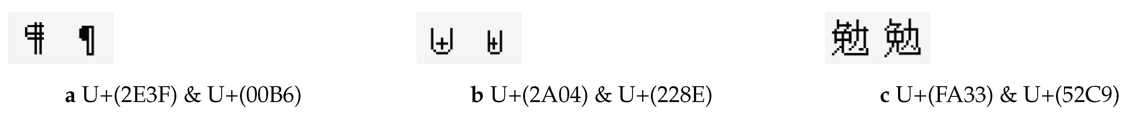
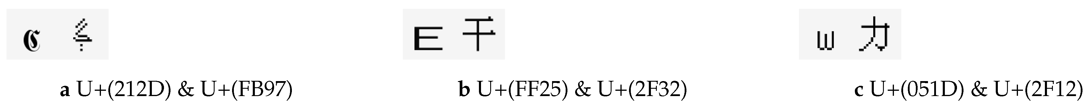
) summarizes the dataset that was used in our experiments. Figure 1 and Figure 2 show several example samples of our dataset.

It is important to note that CJK (Chinese, Japanese, Korean) characters comprise a large portion of Unicode characters. Around $36\%$ of our entire dataset (which is, training, validation, and test dataset) consists of CJK characters. There are 874 CJK characters each in both of the entire similar dataset and dissimilar dataset. Our test dataset is highly dominant with CJK characters. They comprise $46.65\%$ of the dissimilar test dataset and $66.76\%$ of the similar test dataset. Such a comparatively higher ratio in the independent test dataset does not introduce any bias, since they were neither used in training nor in the validation set for hyperparameter tuning.

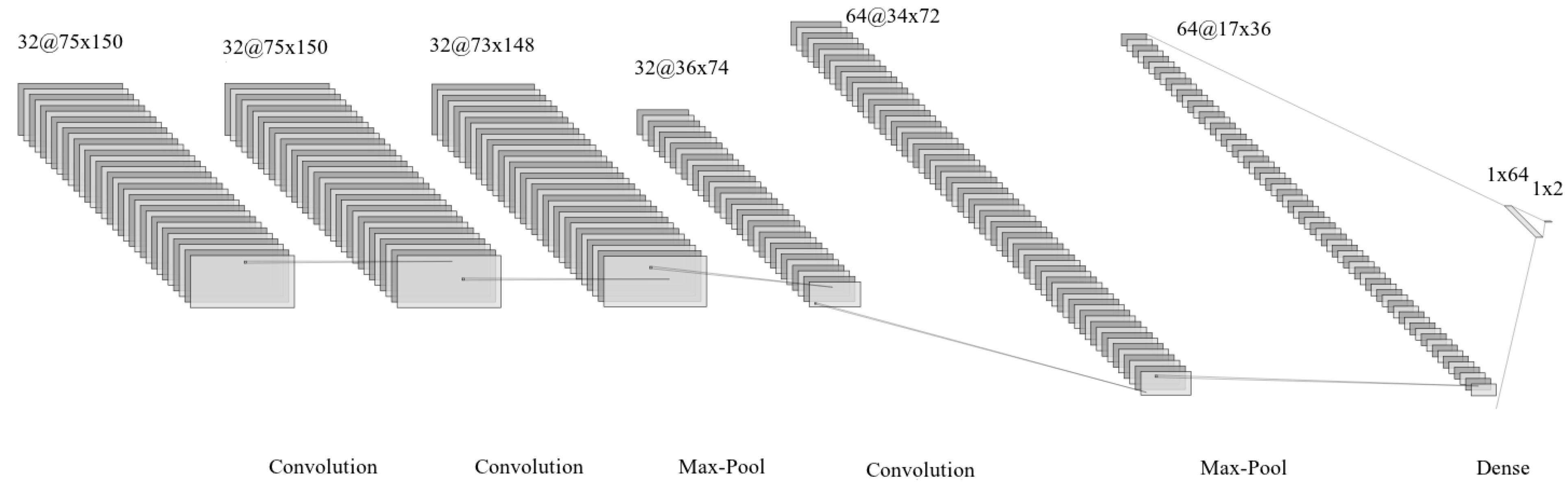
4.2. Proposed Models

We first propose a shallow CNN architecture with two variations to build a model for identifying homoglyphs (Figure 3 and Figure 4, both of which were drawn with the help of the NN-architecture schematics [44]). In the first variation, CNN has four convolutional layers while having two max-pooling layers. The first max-pooling layer comes after the second convolutional layer, whereas the second max-pooling layer comes after the third convolutional layer. The absence of a max-pooling, the layer after the first convolutional layers, is because we want the second layer to learn more complex glyphs’ features based on the first layer’s features. Because maxpooling down-samples an input representation and reduces its dimensionality, the curvy regions of the input image change to linear regions (imagine a semi-circle curve being changed to a right angle). With the assumption that the second layer can learn the representation of curves, we include max-pooling after the second and third layers. In what follows, we refer to this model as ${CNN|}_{Scratch}^1$. The second variation differs from the first, in that we include a dense layer after three convolutional layers. The dense layer is useful here, since we want to ignore spatial information from the previous three convolutional layers. The intuition here is that the similarity of two glyphs also depends on their local features’ similarity. For example, ‘T’ (Cyrillic) and ‘T’ (Latin) should be counted as homoglyph pairs. They both have exactly one horizontal edge on top of a vertical edge. The dense layer is used to count the number of such horizontal and vertical edges (which, in turn, are learned in earlier convolutional layers). Hence, this variation first learns the spatial information of the glyphs and then learns the number in which the spatial features are present to decide whether they are homoglyphs. We call this variation ${CNN|}_{Scratch}^2$. Next, as discussed in Section 2.3, we aim to leverage transfer learning for homoglyph detection by exploiting the features that were learned from several pre-trained models. We will extract features while using pre-trained network weights from popular models. All of these models are state-of-the-art models for ImageNet datasets, and as a result, they already have strong feature extraction capability (for edges, shapes, color blobs, regions, and so on). We refer to this transfer learning-based model as ${CNN|}_{Xfer}$.

5. Experiments

We have conducted extensive experiments while using our dataset. First, we show how several CNN models achieve satisfactory performance on our validation dataset. Then, we justify building an ensembled model and demonstrate that the ensembled model actually perform better in the independent test dataset when compared to the CNN models. After that, we compare our approach to several other techniques in the literature. Finally, we explore various other scenarios, such as artificially augmented test dataset, other pre-trained models for transfer learning, etc.

Table 2. Performance summary (on validation dataset) of the best models in our experiments.

Model	Accuracy	Precision	Recall	F1-Score	MCC
${CNN|}_{Scratch}^1$	0.9883	0.9845	0.9922	0.9884	0.9767
${CNN|}_{Scratch}^2$	0.9861	1.0000	0.9740	0.9868	0.9744
${CNN|}_{Xfer}$	0.9600	0.9255	1.0000	0.9613	0.9255

presents the summary of the results on the validation dataset. As for performance metrics, we have calculated accuracy, precision, recall, F1-Score, and Mathews correlation coefficient (MCC). In what follows, we describe the experiments to analyze our proposed models’ efficiency and efficacy and conduct a comparative study among these models. We also describe a series of preliminary experiments that we have conducted to finalize our different models.

We have experimented with various architectures, built and trained them from scratch, and have observed that networks that rely on smaller filter size perform more consistently than others. In the following subsections, we discuss the two variations of our CNN model built from scratch, i.e., ${CNN|}_{Scratch}^1$, and ${CNN|}_{Scratch}^2$. Subsequently, we discuss our transfer learning-based model ${CNN|}_{Xfer}$. We show that ensembling models in some instances can stochastically have better predictive properties. We conduct independent testing with all of our models. We also compare our results with other SOTA techniques.

5.1. ${CNN|}_{Scratch}^1$

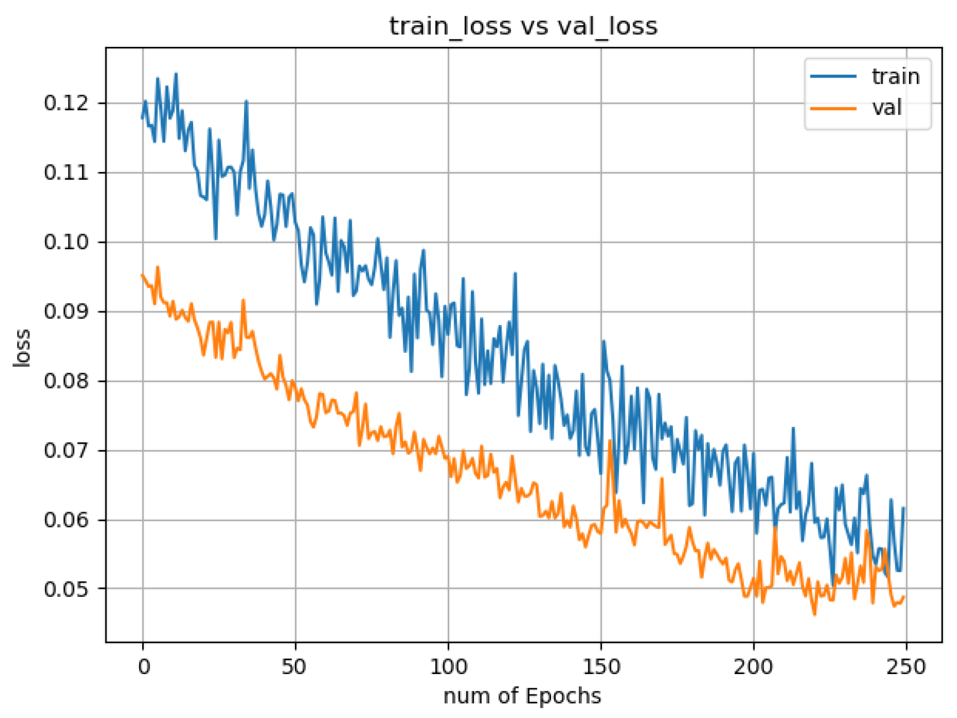
${CNN|}_{Scratch}^1$ utilizes filters with small kernel size ($3\times$ 3). Figure 5 demonstrates the high capability of the model, with accuracy reaching $98.83\%$. The absence of a max-pooling layer after the first convolutional layer means that the model can retain spatial information up to that layer, as discussed before. There is a trade-off between spatial information and dimension-reductional in the latter layers due to max-pooling layers. A reduction in the dimension by max-pooling layers results in a reduced computational cost by reducing the number of parameters to learn and provides basic translation invariance to the input image’s internal representation. However, such a downsampling strategy also means that we lose some spatial information.

Figure 5 also shows that the training and validation curve for the loss function decreases smoothly over time (until it hits a saturation level). An important observation is that the model never was in an overfit state during training. Even though it was slightly underfit, the gap between the training loss and the validation loss remains very little throughout the training phase. Thus, the result justifies the usability of this model and also the proper implementation of training and validation process.

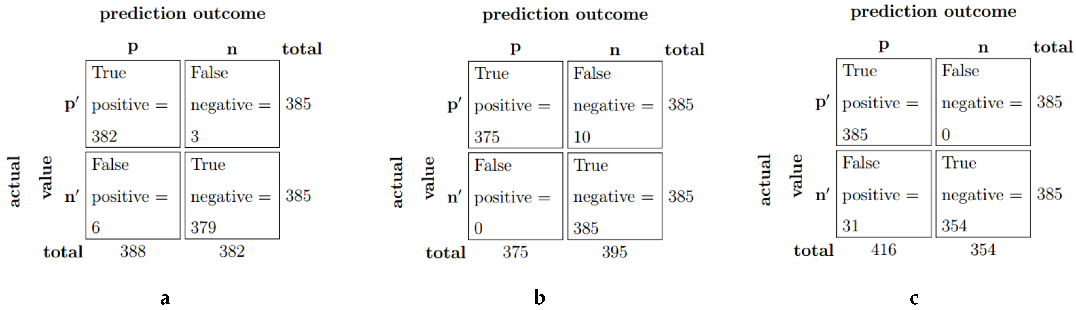
In Figure 6a we report the confusion matrix of of ${CNN|}_{Scratch}^1$ for the validation dataset. A few false positives and false negatives are evident from its 98.45% precision and 99.22% recall value, indicating the model’s strength in detecting both homoglyphs and non-homoglyphs.

5.2. ${CNN|}_{Scratch}^2$

The ${CNN|}_{Scratch}^2$ model differs from the previous model in two aspects: firstly, it contains one less convolutional layer and, secondly, a dense layer replaces the fourth convolutional layer. This allows the model to ignore spatial information. Interestingly, this allows for ${CNN|}_{Scratch}^2$ to have a significant edge over ${CNN|}_{Scratch}^1$ in non-homoglyph detection. Figure 6b presents the confusion matrix of the model. The absence of any false positive sample shows that it correctly identifies all non-homoglyphs. Ignoring spatial information is crucial for the model to have stronger performance (than ${CNN|}_{Scratch}^1$) in non-homoglyphs identification. On the other hand, its performance in identifying homoglyphs drops as compared to the previous model, which confirms that spatial information is more important in identifying homoglyphs. Accuracy-wise ($98.61\%$), this model performs similarly to the previous model accuracy-wise. Notably, all of the convolutional layers here use filters of small kernels with a size of $3\times 3$. Such small receptive fields allow them to detect the letters’ edges and curves more accurately than kernels with higher receptive fields (for example, a kernel of size $5\times 5$).

5.3. ${CNN|}_{Xfer}$

For this model, we have extracted features while using pre-trained network weights from popular models. First, we describe below our experimental findings on the performance of several pre-trained models (after they were fine-tuned).

We leverage VGG-16 architecture, which was pre-trained on the ImageNet dataset [38]. This has a uniform architecture and consists of 16 convolutional layers. We start with the trained network and fine-tune several of the last convolutional blocks of the VGG-16 model alongside the top-level classifier. Subsequently, the unfrozen layers have small weight updates due to the training of the new smaller dataset of ours. We also adopt a very slow learning rate in order to ensure updates of small magnitude.

We have conducted several experiments to identify which layers’ features of the VGG-16 are most potential for our task, and the results are reported in Figure 7 and Figure 8. We do not unfreeze the first five layers, because they capture universal features such as edges, and curves and such features are crucial for our cause. From the Figure 7 and Figure 8, Layer 9 and Layer 12 of the VGG-16 network seem most promising due to a lower loss value. In our experiments, the best model from VGG-16 was achieved utilizing features from Layer 12. Figure 8 shows the accuracy values of the layers during their training. Figure 6c provides clear evidence on the strength of $CNN|Xfer$ in homoglyph detection (based on validation dataset).

Figure 7 and Figure 8 provide us with some interesting insights. Fine-tuning the parameters of the unfrozen layers using transfer learning in our context is slightly harder, as the loss curve for both training and validation fluctuates more when compared to that of Figure 5 . However, as the loss values usually stay within a small range over a large number of epochs (>50), the training is still considered to be stable.

5.4. Ensembled Model

The majority voting is done, as below:

$$f_{ensemble}\left(x\right)=mode\{f_1\left(x\right),f_2\left(x\right),f_3\left(x\right)\}$$

(1)

where, $f_1\left(x\right)$, $f_2\left(x\right)$ and $f_3\left(x\right)$ denotes output, o by ${CNN|}_{Scratch}^1$, ${CNN|}_{Scratch}^2$ and ${CNN|}_{Xfer}$ models respectively. Note that, $o\in \{0,1\}$. $f_{ensemble}\left(x\right)$ is the output of our ensembled model. x is the input image pair. Let us assume that the probability of correctly classifying a homoglyph by ${CNN|}_{Scratch}^1$, ${CNN|}_{Scratch}^2$ and ${CNN|}_{Xfer}$ is $p_1$, $p_2$ and $p_3$ respectively. Additionally, assume that a majority voting process is similarly applied to triple-modular redundancy. The idea is that, even if one of the models misclassifies, the other two can mask the error. Our goal is to increase the probability of correctly classifying a homoglyph by such fault masking. Hence, we want the following condition to be met:

$$\begin{array}{c}\hfill \begin{array}{c}{p}_1{p}_2{p}_3+p_1{p}_2(1-p_3)+p_1(1-p_2)p_3+(1-p_1)p_2{p}_3>p_1(1-p_2)(1-p_3)+\hfill \\ (1-p_1)(1-p_2)p_3+(1-p_1)p_2(1-p_3),\hfill \end{array}\end{array}$$

(2)

where at least two of the models will have the correct output. Recall value of 1.00 of the ${CNN|}_{Xfer}$ model (Table 2) allows us to assume that $p_3\simeq 1$. We can rewrite the above inequaltiy condition as below:

$$\begin{array}{cc}\hfill & p_1{p}_2+(1-p_1)p_2+(1-p_2)p_1>(1-p_1)(1-p_2)\hfill \\ \hfill \Rightarrow & 2p_1+2p_2>1+2p_1{p}_2\Rightarrow p_1+p_2-p_1{p}_2>\frac{1}{2}\hfill \end{array}$$

(3)

$p_1+p_2-p_1{p}_2=\frac{1}{2}$ represents a hyperbola of the form $x+y-xy=\frac{1}{2}$ or $y=\frac{1-2x}{2-2x}$.

The black region that is bounded by the hyperbola in Figure 9 indicates the condition in (3) being unsatisfied. The area of the black region is:

$$\begin{array}{cc}\hfill {\int }_0^{\frac{1}{2}}dy& ={\int }_0^{\frac{1}{2}}\frac{1-2x}{2-2x}dx={\left[x+\frac{1}{2}log(1-x)\right]}_0^{\frac{1}{2}}=\frac{1}{2}(1+log\frac{1}{2})=0.3494\hfill \end{array}$$

Therefore, the white region area is $1-0.3494=0.6506>0.5$, which indicates that the majority voting of the ensembled models improves the detection of homoglyphs. Table 2 also displays precision value of the ${CNN|}_{Scratch}^2$ model being $1.00$. Following the same argument as above, ensembling the models is more likely to yield better accuracy in detecting non-homoglyphs. This is further strengthened by the experimental analysis that is discussed below.

Clearly ${CNN|}_{Scratch}^1$ exhibits superior performance (100% specificity, or true negative rate (TNR) in the validation dataset) in detecting non-homoglyphs. However, its 96.80% recall rate suggests that it can not always detect homoglyphs. On the other hand, ${CNN|}_{Xfer}$ exhibits 100% recall in detecting homoglyphs while misclassifying several non-homoglyphs as homoglyphs (which is evident from its 94.60% precision in the validation dataset). On the other hand, ${CNN|}_{Scratch}^2$ has both high precision and recall values.

Table 3. Verdict on the three models.

Model	Pros	Cons
${CNN|}_{Scratch}^1$	Strong at detecting both homoglyphs and non-homoglyphs	Neither Precision nor Recall is 1.00
${CNN|}_{Scratch}^2$	Very strong at detecting non-homoglyphs	May miss a few homoglyphs
${CNN|}_{Xfer}$	Very strong at detecting homoglyphs	May misclassify some non-homoglyphs as homoglyphs.

summarizes the strengths and weaknesses of the three models.

Because detecting homoglyphs is of utmost priority (i.e., there should not be any false negatives), we can not wholly rely on ${CNN|}_{Scratch}^1$, or ${CNN|}_{Scratch}^2$, despite its very high accuracy (our validation result from Table 2 shows that these two have higher accuracy than the ${CNN|}_{Xfer}$ model).

This allows for the decision module (applying majority voting) to mask any faults in prediction potentially. Such a fault-tolerant approach allows us to potentially overcome the mistake/fault by a single module since the other two do not make a faulty prediction. Figure 10 displays the final ensemble model.

5.5. Independent Testing

This section evaluates the performance of our ensemble model in the test dataset. The modules are also tested individually in order to see how they would perform as a stand-alone module. The goal is to check how well our models perform when presented with a previously unseen glyph set. This evaluation’s performance will indicate that our model is generalized and robust enough to detect homoglyphs in real-life scenarios as and when new homoglyphs are/will be introduced.

Table 4. Performance summary of the final ensemble model and the individual modules on the test dataset.

Model	Accuracy	Precision	Recall	F1-Score	MCC
Ensembled Model	0.9972	1.0000	0.9944	0.9972	0.9944
${CNN|}_{Xfer}$	0.9274	0.8732	1.0000	0.9323	0.8639
${CNN|}_{Scratch}^1$	0.9944	1.0000	0.9888	0.9944	0.9889
${CNN|}_{Scratch}^2$	0.9944	1.0000	0.9888	0.9944	0.9889

reports the performance comparison.

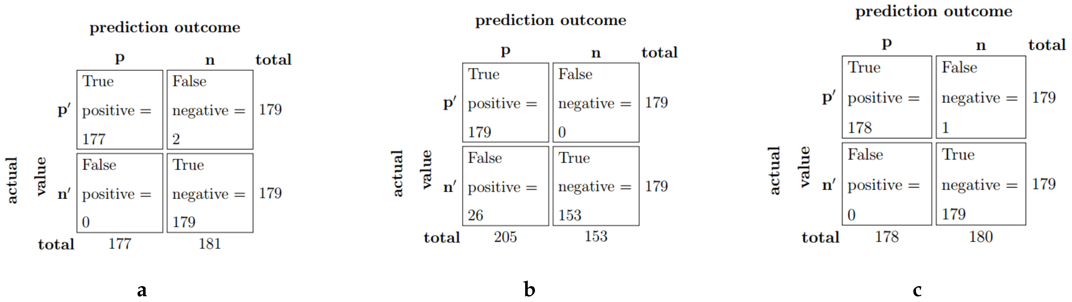
5.5.1. Ensembled Model Performance

Figure 11c shows the confusion matrix of our ensembled model on the test dataset. The model achieves 99.72% accuracy, with one sample being a false negative. Both ${CNN|}_{Scratch}^1$ and ${CNN|}_{Scratch}^2$ mistakenly identify the (originally homoglyph) glyph pair as non-homoglyphs.

Figure 12 shows the false negative sample.

5.5.2. ${CNN|}_{Xfer}$ as a Stand-Alone Model

We also experiment while using ${CNN|}_{Xfer}$ independently. From Figure 11b, we see that there is no false negative prediction by ${CNN|}_{Xfer}$ in the test dataset. However, there are some false positives. Hence, this model correctly predicted labels of all the homoglyphs. The result is similar to its performance in the validation dataset. It mostly had trouble with CJK Unified Ideograph and CJK Radical Supplement character pairs (see Supplementary Materials).

Our observation is that learning similarity features of homoglyphs is much easier for ${CNN|}_{Xfer}$ than learning dissimilarity features. ${CNN|}_{Xfer}$ has a deep 16-layer architecture, unlike ${CNN|}_{Scratch}^1$ and ${CNN|}_{Scratch}^2$, which are shallow CNNs. It exhibits stronger performance in detecting homoglyphs, whereas ${CNN|}_{Scratch}^1$ and ${CNN|}_{Scratch}^2$ exhibit stronger performance in detecting non-homoglyphs.

5.5.3. ${CNN|}_{Scratch}^1$ and ${CNN|}_{Scratch}^2$ as Stand-Alone Models

Stand-alone ${CNN|}_{Scratch}^1$ performs much better than stand-alone ${CNN|}_{Xfer}$ in the test dataset, as is evident from its 99.44% accuracy along with 100% precision. There are two samples where the former fails to successfully classify them as homoglyphs. One of them is a CJK Compatibility Ideograph and CJK Unified Ideograph pair and another one is a CJK Radical Supplement and CJK Unified Ideograph pair.

Stand-alone ${CNN|}_{Scratch}^2$ performs similarly to stand-alone ${CNN|}_{Scratch}^1$. In fact, they exhibit identical confusion matrix (Figure 11a). However, the sets of false negatives are different for the two models. In particular, stand-alone ${CNN|}_{Scratch}^2$ also misclassifies the sample in Figure 12. It correctly classifies the CJK Radical Supplement and CJK Unified Ideograph pair that stand-alone ${CNN|}_{Scratch}^1$ misclassified, as seen in Figure 12. The other pair that it misclassified is a CJK Unified Ideograph and CJK Unified Ideograph pair. The inaccurate classifications by the stand-alone models can be seen in Figure 13.

5.5.4. Comparison with Other Techniques

Once we have ensembled our final model, we demonstrate the model’s classification ability by comparing it with other state-of-the-art image similarity techniques. Note that we have manually prepared a dataset following a systematic approach. We have evaluated other image similarity-based techniques on the same dataset for a fair comparison.

Table 5. Comparison of performance with image similarity based techniques on our dataset. Structured Similarity Index Metric (SSIM), Pixel_Sim, Scale-Invariant Feature Transform (SIFT), and Earth Mover’s Distance (EMD) denote the support vector machine (SVM) models which were built while using the respective features.

	Accuracy	Precision	Recall	F1-Score
SSIM [25]	0.56	0.66	0.23	0.34
Pixel_Sim [46]	0.64	0.79	0.39	0.52
SIFT [26]	0.5	0.5	1	0.67
EMD [27]	0.67	0.60	1	0.75
Siamese1 [22]	0.26	1	0.51	0.67
Siamese2 [23]	0.48	0.34	0.4	0.37
AlexNet [38]	0.91	0.89	0.93	0.91
LeNet [47]	0.92	0.91	0.93	0.92
Our Ensembled Model	0.9972	1	0.9944	0.9972

reports the results. In particular, we have reported the accuracy, precision, recall, as well as the F1-score.

Structured Similarity Index Metric (SSIM) [25] is a method for measuring the similarity between two images. Usually, it gives a score within a range of $-1$ to 1, where a higher value means more similarity and a lower value means more dissimilarity. We calculate SSIM values for our pair of glyphs and stores them as features. We build a Support Vector Machine (SVM) model that is trained with these features and finally evaluate on our test dataset. Unfortunately, 56% accuracy on the test dataset shows that the SSIM scores are not suitable for our task at hand.

Next, being inspired by the approach of [46], we compute pixel similarity among glyphs. In particular, we use the normalized absolute difference value of the pixels. Using these values as features, we build another SVM model, henceforth referred to as Pixel_Sim. The performance metrics clearly show that such a simple feature is, in fact, better than SSIM. However, the result is not satisfactory at all as compared to our final ensemble model.

Similarly, Scale-Invariant Feature Transform (SIFT) [26] and Earth Mover’s Distance (EMD) [27] algorithms are exploited for extracting features for SVM models in a similar manner. In the first case, we first extract keypoints and descriptors. We initialize a Bruteforce matcher with normalized Hamming distance to find similar regions based on the extracted keypoints and descriptors. We use the normalized distance as feature for our SVM model. SIFT based features do not yield acceptable results, as seen in Table 5. In the second case, we take inspiration from [27] and measure EMD between glyphs’ pairs. Again, we use this measurement as features for another SVM model, achieving an accuracy of only 67%. It implies that we cannot use EMD between two glyphs as a reliable feature for detecting homoglyphs.

Next, we compare our results with Siamese Convolutional Neural Network based methods reported in [22,23]. We train both Siamese Neural Networks on our dataset. However, in our experiments, we observe that the generated models are highly overfitting. With the method of [22], we achieve approximately 99.50% training accuracy, but only 25% validation accuracy on average. We observe a similar overfitting phenomena with the method of [23], even with a very low number (4–8) of feature maps per convolutional layer. However, in this case, the difference between the training and validation accuracy is about 15% on average. We observe that both of the approaches have very poor accuracy when trained on our dataset. Notably, to keep our comparisons as fair as possible, we refrain from applying data augmentation in both of these approaches.

A brief discussion on why the methods of [22,23] perform poorly in our context is in order. Intuitively, the reason for a poor performance by the method of [22] can be attributed to the fact that its architecture has been fine-tuned for images that contain the whole URL as an image. On the contrary, in our case, our model learned to distinguish two-character glyphs in a visual manner. As a result, it is safe to say that their Siamese neural network was built for a more complex image dataset, resulting in overfitting when applied in our context. As for the method of [23], we believe that the network’s architecture is too complex for our task at hand. This is evident from the fact that the results were not improving, even after reducing the number of filters per layer.

Finally, we test the effectiveness of Alexnet [38] and LeNet [47]. Both of them perform worse when compared to our results. From an empirical study, we found that both filters with higher size and CNN with 5 or more layers have a poor impact on the result. Alexnet and LeNet exploit filters of $11\times 11$ and $5\times 5$ size, respectively. LeNet also uses the tanh activation function, which performed poorly in our experiments.

5.5.5. Comparison with OCR Based Techniques

OCR based techniques are trained to recognize a pre-defined set of characters. To determine if two Unicode characters form a homoglyph pair, both of the characters are taken as input to an OCR module and checked whether both of them are considered to be the same character. In case both are treated as the same character, the pair is labeled as a homoglyph pair. Otherwise, the pair is labeled as a non-homoglyph pair. An OCR module is required to recognize all Unicode characters in existence to determine whether a new character forms a homoglyph pair with any of them, as discussed in Section 3. Due to such limitations, we only work with CJK characters for experimental purposes. We compare our performance against the studies in [48].

The authors in [48] train their model to learn Chinese word representations from the bitmaps of character glyphs with a convolutional auto-encoder with two main steps, as follows. Firstly, the authors extract character glyph features with the help of an convolutional auto-encoder. Secondly, using the features that were obtained from the first step, Chinese word representations are learned. We emulate their approach, as stated in the first step for OCR based comparison. The extracted character glyph features are directly used to classify Chinese characters.

Out of all CJK homoglyph pairs from our test dataset, we randomly choose 100 pairs. We also choose 100 non-homoglyph pairs randomly, irrespective of which alphabet/script they are from. The OCR modules are trained in order to recognize at most one character glyph from a homoglyph pair. Trained glyphs belong to the Chinese alphabet and untrained glyphs belong to Hangul, Yi syllables, Yi radicals, Kangxi radicals, Katakana, miscellaneous technicals etc. To detect a homoglyph using OCR technique, we pass both of the characters into the OCR model as input at first and notice whether they are classified as the same character class.

Table 6. Comparison with OCR based techniques. We focus on CJK characters only due to OCR techniques being limited to the number of characters it can classify.

Model	Accuracy	Precision	Recall	F1-Score
Approach in [48]	0.9650	1.0000	0.9300	0.9637
Our Ensembled Model	0.9972	1	0.9944	0.9972

shows that our ensembled model outperforms both of the OCR based approaches. We find that the performance of both approaches deteriorates when they are given low-resolution character glyphs as input. As a result, we had to separately resize the datasets to enhance their performance. We also observe that performance degrades for both these models when the images of the two glyphs to be compared had different sizes. Figure 14 presents several homoglyph pairs that were troublesome for both of the OCR methods. Because OCR models are usually trained with characters that are usually similar in size, they are less robust to inputs with varying size. However, our model is trained to detect two glyphs similarity no matter which script they belong to or whatever the size of their image be.

5.5.6. Testing on Augmented Dataset

Our test dataset being small (179 instances for both classes) may not truly reflect our ensembled model’s capability. In order to address the issue, we artificially augment our test dataset with the following transformations:

• Rotation (The rotation can be from −10° to 10°.)
• Scaling (a scaling factor of $0.9$ to $1.1$ is applied. Anti-aliasing is applied if the image is being downscaled.)
• Horizontal flipping (a horizontally flipped homoglyph pair should remain a homoglyph pair. The same can be said true for non-homoglyphs.)
• Vertical flipping (the same reasoning as above can be applied here.)

We also induce random noise by randomly setting pixels to white or black. In the case of setting pixels to white, $1\%$ of the pixels were randomly set, whereas, in the case of setting pixels to black, $5\%$ of the pixels were chosen. We set more pixels to black than white because the character glyphs are dominant with white background. We apply the transformations mentioned above to generate the augmented test dataset. The probabilities of a glyph pair being chosen and a transformation to be applied are uniform. Additionally, the rotation and scaling factors may vary between the glyphs within a glyph pair. However, flipping and noising are kept consistent, so that the relationship (similar or dissimilar) between the glyphs is also consistent. The comparison is shown in

Table 7. Our augmented test dataset is four times the original dataset. Therefore, there are 716 similar/homoglyph pairs and 716 dissimilar/non-homoglyph pairs. The augmented test dataset is originated from the original test dataset.

	Accuracy	Precision	Recall	F1-Score
Augmented test dataset	0.9972	1.00	0.9944	0.9972
Original test dataset	0.9986	1.00	0.9972	0.9986

. Evaluating the individual predictions of the glyph pairs reveal that the model behaves exactly similar in both cases. The higher accuracy and F1-score in the augmented test dataset are because the homoglyph pair in Figure 12 was transformed only twice instead of four times (which is the mean of the number of transformations for all glyph pairs). In a separate experiment, we apply k-fold validation (where $k=3$) and find that our ensembled model achieves 99.63% accuracy on average.

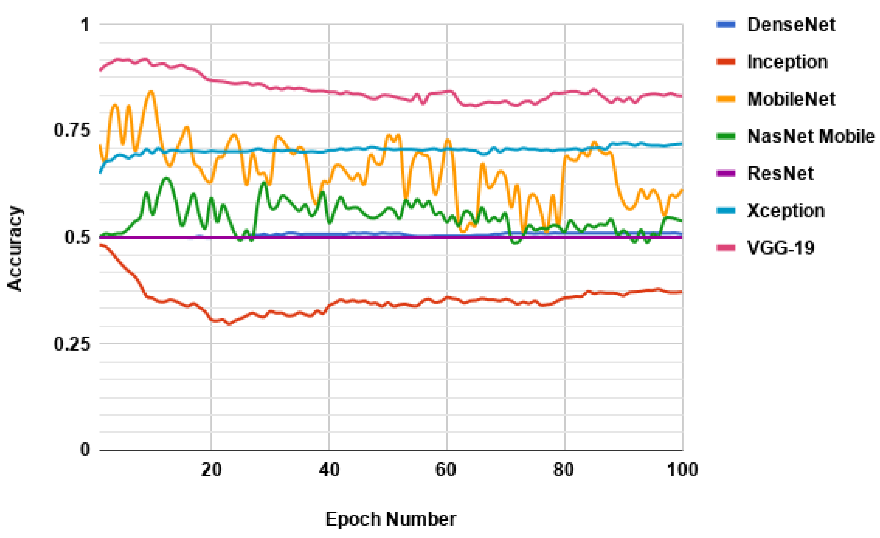
5.5.7. Performance of ${CNN|}_{Xfer}$ Module with Other Pre-Trained Models

We replace VGG-16 network with other pre-trained networks for the ${CNN|}_{Xfer}$ module. VGG-19 [37], ResNet [40], NasNet [49], MobileNet [50], Inception Network [51], XceptionNet [52], and DenseNet [53] are the most used pre-trained networks in computer vision for transfer learning. VGG-19 network resembles the VGG-16 network most (which was used in our ${CNN|}_{Xfer}$ module), except that it contains three more layers. The other models mentioned above are more complex in nature. They also contain many more layers than VGG-16, and hence can be considered deeper networks.

Figure 15 shows the result when the VGG-16 network is replaced with these networks. Deep networks perform far worse than those that use a fewer number of layers. For example, the VGG-19 network has almost identical performance to that of the VGG-16 network. It has 91.80% validation accuracy, which is 4:20% less than the VGG-16 network. Other networks achieve 65.43% accuracy on average. Only the accuracy of the mobilenet crosses 80% threshold in our experiments. Xception is the closest in performance with around 72.14% accuracy. All others achieve an accuracy closer to 50%. Because this is a binary classification with an equal number of training and validation samples, 50% can be the least possible accuracy and, hence, is the baseline for our experiments. 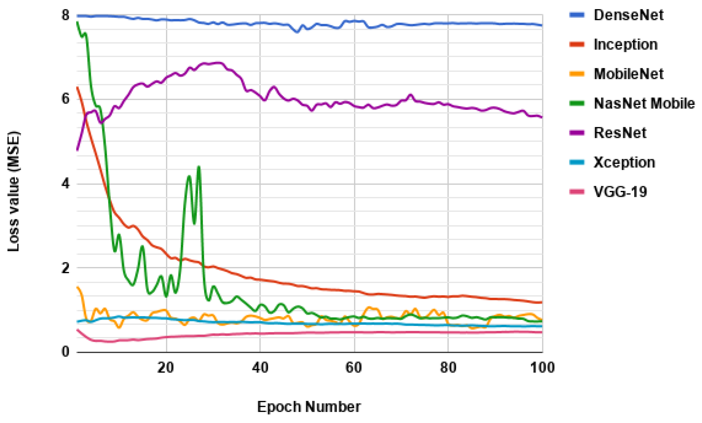Figure 16 reports the training of the models.

Figure 16 shows the instability of the transfer learning based approach for many of the architectures. For example, the loss value of DenseNet is unreasonably high as its value tends to stay close to $8.0$. Same can be said for ResNet. Other models exhibit smoother training. In fact, all the models used in our ensembled model have smooth training, as seen from Figure 5, Figure 7 and Figure 8. On the other hand, most of the models that we excluded exhibit non-smooth training or non-convergence, as seen in Figure 16. Thus, this result justifies our selection of model.

5.5.8. Other Observations

We choose Stochastic Gradient Descent (SGD) as the optimizer based on its performance on a series of experiments. We fix all the hyperparameters except optimizers. We train the models several times for each optimizer and measure the average accuracy for all of them. Figure 17 indicates that, although they are almost identical in performance, SGD is slightly better than others.

Another observation from our experiments is that restricting the size of the filters to $3\times 3$ achieves best performance. Filters of size $5\times 5$ and $7\times 7$ obtain 96.02% and 95.04% accuracy on average, respectively, when used in our ${CNN|}_{Scratch}^1$ module.

6. Conclusions

We have developed a deep learning based model for discovering homoglyphs as a preventive defense mechanism that is expected to be useful against different attacks, like phishing, ID impersonation, etc. Our final model is an ensemble of three separate models. We first exploit a shallow CNN architecture with limiting max-pooling layers in order to retain spatial information to predict if two glyphs are similar. This model, referred to as ${CNN|}_{Scratch}^1$, shows 100% accuracy in detecting non-homoglyphs in our test dataset. We also show that ignoring spatial information with a dense layer (while also exploiting shallow CNN architecture) achieves high-performance in terms of accuracy. This model, referred to as ${CNN|}_{Scratch}^2$, exhibits strong performance in both homoglyph and non-homoglyph detection. We also leverage transfer learning from the VGG-16 network to build a model, called ${CNN|}_{Xfer}$, which can detect homoglyphs with 100% accuracy. The developed model’s contrasting performance in homoglyph vs. non-homoglyph detection inspired us to build an ensemble model. Our ensemble model, applying a majority voting policy on three other models’ output, registers its robust capability as a homoglyph detector model.

The purpose of this research is to provide a classifier that can be used for discovering homoglyphs. Section 5.5 shows that our model is highly accurate in detecting whether a pair of glyphs is a homoglyph. Such checks can be carried out offline, given that a user using the model has access to fonts that are capable of rendering glyphs of the characters. However, in the case of real-time defense, an application should already have a list of homoglyphs in hand. Modern browsers, with the help of punycodes [54], can detect phishing links/URLs with some limitations. One exciting use of our model could be to suggest and produce a list of potential phishing links/URLs from a given link. This has several benefits, including, but not limited to, creating a database as a preventive defense mechanism for phishing attacks in the browser. Organizations, like banks, can also carry out awareness initiatives and prevent their users from inadvertently clicking phishing URLs. Our model can also be exploited to assign a threat level to a partial link/URL. We estimate the threat level by looking at the output of softmax probabilities of the last layer. We define the predicted class’s softmax probability output as the confidence with which our model predicts a homoglyph (or a non-homoglyph). The more confidence our model has in detecting a homoglyph, the higher the threat level is for the pair. Thus, a link can be assigned a threat level based on the characters that it contains.

In future, we aim to expand the detection of similarity to more general cases, such as handwriting recognition, signature verification, etc.