Finite Cascades of Pitchfork Bifurcations and Multistability in Generalized Lorenz-96 Models


Bernoulli Institute for Mathematics, Computer Science, and Artificial Intelligence, University of Groningen, P.O. Box 407, 9700 AK Groningen, The Netherlands
*
Author to whom correspondence should be addressed.
†
These authors contributed equally to this work.
Math. Comput. Appl. 2020, 25(4), 78; https://0-doi-org.brum.beds.ac.uk/10.3390/mca25040078
Submission received: 12 November 2020
/
Revised: 5 December 2020
/
Accepted: 7 December 2020
/
Published: 9 December 2020
(This article belongs to the Section Natural Sciences)
Abstract
:In this paper, we study a family of dynamical systems with circulant symmetry, which are obtained from the Lorenz-96 model by modifying its nonlinear terms. For each member of this family, the dimension n can be arbitrarily chosen and a forcing parameter F acts as a bifurcation parameter. The primary focus in this paper is on the occurrence of finite cascades of pitchfork bifurcations, where the length of such a cascade depends on the divisibility properties of the dimension n. A particularly intriguing aspect of this phenomenon is that the parameter values F of the pitchfork bifurcations seem to satisfy the Feigenbaum scaling law. Further bifurcations can lead to the coexistence of periodic or chaotic attractors. We also describe scenarios in which the number of coexisting attractors can be reduced through collisions with an equilibrium.
1. Introduction
The Lorenz-96 model, which was constructed by E.N. Lorenz [1], is a frequently used toy model in studies that are related to predictability and weather forecasting. The so-called monoscale version of the model is given by the equations
where the indices of the variables are taken modulo a fixed integer :
Equation (2) can be interpreted as a periodic boundary condition. In fact, Lorenz [1] interpreted the variables as values of some atmospheric quantity in n equispaced sectors of a latitude circle, where the index j plays the role of longitude. The dimension and forcing parameter are free parameters.
Low-dimensional atmospheric models that were used in earlier predictability studies, such as the Lorenz-63 and Lorenz-84 models, were derived as Galerkin projections of partial differential equations describing the laws of physics [2,3,4,5]. In contrast, the Lorenz-96 model was not constructed as a physically realistic model, but rather as a model that is easy to use in numerical experiments. Nevertheless, the model has physically relevant components, such as advection terms, damping terms, and external forcing. The feature that the dimension n of the model can be chosen arbitrarily large allows for much richer dynamics in comparison to the aforementioned Lorenz-63 and Lorenz-84 models. The latter property has made the Lorenz-96 model an attractive model for studies on forecasting [6,7,8,9], predictability [10,11,12], high-dimensional chaos [13,14,15,16], and data assimilation schemes [17,18,19,20].
The broad interest in the Lorenz-96 model has inspired several authors to introduce and study modifications of the model. Kerin and Engler [21] identified the desired properties for the nonlinear advection terms and provided a classification of all advection terms that are quadratic, energy-preserving, and equivariant with respect to circulant permutations of coordinates, and localized up to some degree. Vissio and Lucarini [22] supplement the Lorenz-96 model with temperature-like variables. This addition allows for the existence of an energy cycle, in which conversion between kinetic and potential energy is possible.
In this paper, we introduce our own variant of the Lorenz-96 model. Instead of deriving our modification from physical considerations, we stay closer to the structure of the nonlinear terms in Equation (1). Specifically, we modify the nonlinear terms by simply changing indices: for a given triple , we consider the system
which is again subject to the condition in Equation (2). Note that the boundary condition in Equation (2) implies that the numbers , , and can always be taken modulo the dimension n, whenever this is necessary. In the remainder of this paper, these systems will be identified by the symbol . Note that is just the original Lorenz-96 model of Equation (1). The dynamics of the latter model has been studied in detail in the papers [23,24,25]. A particular phenomenon that was discovered was the succession of pitchfork bifurcations, which, in combination with further bifurcations, leads to the coexistence of attractors. The main purpose of this paper is to determine what extent this scenario occurs in the systems . Rather than providing an exhaustive analysis of all possible cases, we will highlight the differences and similarities for three concrete choices of .
This paper is structured, as follows. In Section 2, we first discuss some general properties of the system , such as the boundedness of orbits and stability properties. In Section 3, we first derive sufficient conditions under which a pitchfork bifurcation occurs. Next, we numerically investigate whether the first pitchfork bifurcation is followed by a cascade of such bifurcations. Section 4 shows how pitchfork bifurcations in conjunction with other bifurcations lead to the coexistence of periodic or chaotic attractors. Section 5 concludes the paper with a discussion of the open questions that arise from our results.
2. General Properties
In this section, we study the properties that all members of the family have in common, such as boundedness of orbits and the stability of equilibria.
2.1. Boundedness of Orbits
In this section, we determine sufficient conditions under which orbits of the system remain bounded for all time. This is a necessary first step, since, unlike the generalized Lorenz-96 models that were introduced in [21], the quadratic advection terms in our model do not necessarily preserve the total energy. Although unbounded orbits are not of physical relevance, they can still appear in physically relevant models, such as those that are derived from the shallow water equations, see [26,27].
The discussion in this section closely follows the arguments that are presented in [26]. Let
denote the unit sphere in and define the following quantities:
where we take the indices of the variables modulo n. Note that , since both of the quantities are obtained by maximizing a polynomial of odd degree. If we define , then it follows that
which implies that
Now, assume that , or, equivalently,
If , then this condition trivially holds and whenever , which means that the orbits of the system are bounded for all . If , then whenever , where
Orbits for which for some satisfy for all , which gives a sufficient condition for the boundedness of orbits. Orbits for which for some are potentially unbounded. Hence, we are mainly interested in the region .
The next question is for which the values of n and F the condition in Equation (4) holds. For the original Lorenz-96 model , it can be easily verified that for all , which, in particular, implies that all of the orbits are bounded. Another example is given by the system . More generally, if the system has the property that for all , then so does the system . However, for some systems, it may occur that for some . A concrete example is the system for which when , but when . In such cases, it is useful to know how and vary with n in order to check the condition in Equation (4).
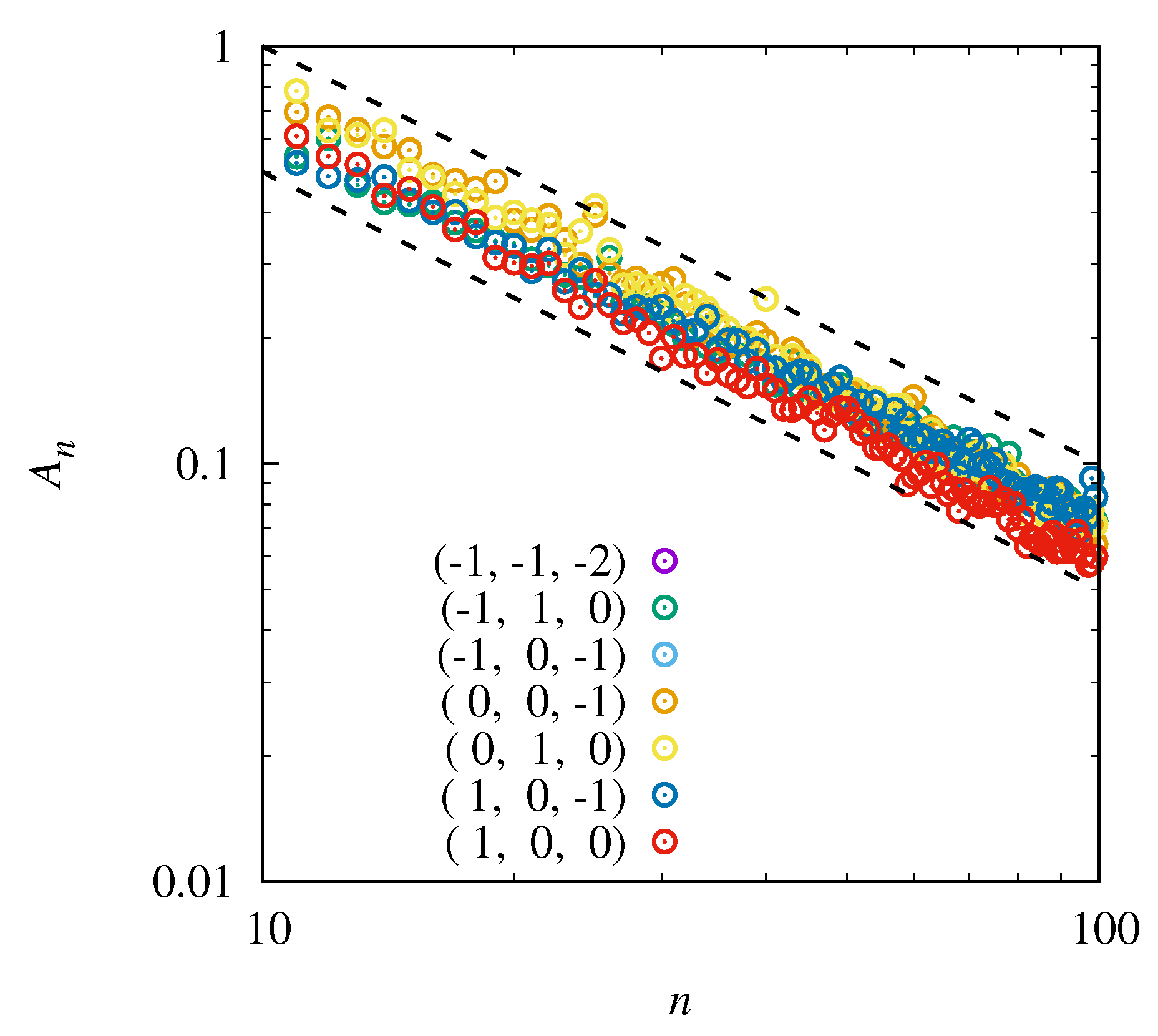
The equality case of the Cauchy–Schwarz inequality implies that . However, an exact expression for the quantity is not so easy to derive analytically: for example, when applying the method of Lagrange multipliers, a system of quadratic equations needs to be solved as a result of the cubic terms in the expression for . Therefore, we perform a numerical experiment in order to determine the dependence of on n. For a fixed choice of and n, the quantity is approximated by taking the largest value of the sum
over randomly chosen points . These maxima are plotted as a function of n in Figure 1; increasing the number of points in the maximization procedure only produces very minor differences. The figure clearly suggests, for several choices of the triple , that with , which implies that . In these cases, the condition presented in Equation (4) will be satisfied for sufficiently large n and sufficiently small . Moreover, a larger n allows for a larger value of .
Note that Figure 1 only shows the results for small values of the triple . For the larger range , the decay of with n is the same as in Figure 1 (not shown). In the remainder of this paper, we will restrict ourselves to small values of . This is motivated by the observation that the Lorenz-96 model and its generalizations shown in Equation (3) have a similar structure as finite-difference discretisations of partial differential equations in which the interaction between the nonlinear terms are often local in nature; also see the discussion in [21].
2.2. Stability of Equilibria
All of the systems have an equilibrium solution that is given by . The eigenvalues of the Jacobian matrix at this equilibrium can be expressed explicitly in terms of and n, as the next result shows.
Lemma 1.
The eigenvalues of the Jacobian matrix of at are given by
where
Moreover, the eigenvector corresponding to the eigenvalue is given by
where are the n-th roots of unity.
Proof.
Without a loss of generality we may assume that . Note that the Jacobian matrix of System (3) evaluated at is circulant, which means that each row is a cyclic right shift of the row above. If we denote the first row by , then it follows from [28] that the eigenvalues and corresponding eigenvectors are given by
Because we have that , , , and for all , it follows that
This completes the proof. □
Note that the parameter does not influence the stability of the equilibrium . Hence, in the remainder of the paper, we will mainly focus on the case . The next result follows directly from Lemma 1.
Proposition 1.
For a fixed integer , we have the following:
- If for some , then and, hence, the eigenvalue cannot cross the imaginary axis upon varying F. In particular, if , then for all , which implies that the equilibrium is stable for all .
- If for some , then the eigenvalue will cross the imaginary axis at the parameter value .
- If for all , then bifurcations of the equilibrium can only occur for . In particular, this holds when .
- If for all , then bifurcations of the equilibrium can only occur for . In particular, this holds when .
Lemma 1 also implies that the equilibrium is stable for sufficiently small. The shape of the graphs of the functions and strongly determines the nature of the first bifurcation of .
2.3. Degenerate Cases
For specific choices of , the bifurcations of the system can be degenerate. For example, consider the system . If , where , Lemma 1 implies that for , which means that the equilibrium becomes unstable by two real eigenvalues crossing zero. The occurrence of a Bogdanov–Takens bifurcation can be ruled out, since the Jacobian matrix at is diagonalizable [29]. In fact, the next result shows that two lines of equilibria appear at .
Proposition 2.
For system with and , the following sets are equilibrium solutions:
Proof.
For , the right hand side of System (3) reads as
A vector belongs to if and only if one the following cases is satisfied:
- ;
- ;
- ; and,
- .
Straightforward computations show that, in each of theses cases, for all . This proves that elements of are indeed equilibria of System (3). The proof for is similar. □
The previous result implies that the equilibrium undergoes a degenerate bifurcation at . For , the equilibrium is unstable and numerical experiments show that orbits can become unbounded when their initial point is not contained in a compact invariant set, such as an equilibrium or periodic orbit.
The occurrence of multiple zero eigenvalues is not limited to the specific system . More generally, the Jacobian matrix of the system at has precisely eigenvalues that are equal to zero when n is a multiple of and . Indeed, if and , then Lemma 1 implies that the eigenvalues are given by
Solving the equation for gives
The restriction leads to the restriction . Hence, if divides n, then there precisely exist integers for which .
In the remainder of this paper, we will only consider systems for which degeneracies, as described above, do not occur.
3. Finite Cascades of Pitchfork Bifurcations
In this section, we first discuss under which conditions on the triple the equilibrium loses stability through a pitchfork bifurcation. Next, we discuss the resulting bifurcation scenario for specific choices of . Rather than providing an exhaustive analysis of all possible cases, we will restrict the discussion to three concrete examples. In particular, we discuss to what extent these examples differ from the original Lorenz-96 system.
3.1. Conditions for a First Pitchfork Bifurcation
For to loose stability through a pitchfork bifurcation, it is necessary that one of the eigenvalues equals zero, whereas all other eigenvalues have a negative real part. A sufficient condition on for which this holds is given in the next result.
Proposition 3.
Assume that, for , the function
attains a unique global maximum or minimum on the interval at . Subsequently, it follows that:
- If n is odd, then zero eigenvalues of the equilibrium must occur at least in pairs; and,
- If n is even, then one eigenvalue equals zero for , whereas the other eigenvalues have a negative real part.
Proof.
Recall, from Lemma 1, that the eigenvalues , where , of satisfy . It is straightforward to check that . This implies that , which means that eigenvalues cross the imaginary axis in pairs.
When n is even, it follows that for . Because is assumed to have a unique global maximum or minimum at , it immediately follows that all of the other eigenvalues have a negative real part at . □
It is straightforward to verify that the Lorenz-96 model satisfies the conditions of Proposition 3. Other choices of given by , , and which will be discussed in more detail below. In addition, observe that
Therefore, if the equilibrium loses stability through a zero eigenvalue crossing, then this will necessarily occur at or .
A zero eigenvalue crossing is a signature of a saddle-node bifurcation, a transcritical bifurcation, or a pitchfork bifurcation. The saddle-node bifurcation can be ruled out, since the equilibrium continues to exist after the eigenvalue crossing has taken place. However, further analysis is needed in order to distinguish between a transcritical and a pitchfork bifurcation. A typical approach is to compute a normal form while using a center manifold reduction [29], but these computations are rather long. For the Lorenz-96 model, such computations are provided in [30], but below we shall adopt a more elementary and quicker approach. The next result shows, for certain members of the family , a supercritical pitchfork bifurcation of the equilibrium takes place when and .
Proposition 4.
If , with , then it follows that, for the systems , , and , the equilibrium loses stability through a supercritical pitchfork bifurcation at , while, in the system , a supercritical pitchfork bifurcation occurs at .
Proof.
As an ansatz, we assume that System (3) has an equilibrium of the form , in which case by circulant symmetry is also an equilibrium. For the system , it then follows that
Of course, is a solution, but this would lead to the already known equilibrium . Solving a from the first equation gives , so that the second equation yields a cubic equation for b:
If , , and denote the roots of the latter equation, then Vieta’s formulas give
Without loss of generality, we can take , in which case we find
Solving and from these equations is straightforward and it gives the following expressions for a and b:
This means that, for , two new equilibria appear that coalesce with at . Because the two new branches of equilibria extend in the direction, in which becomes unstable, we conclude that a supercritical pitchfork bifurcation takes place.
For the systems and , we obtain the same result and, therefore, the computations are omitted. For the system , we obtain the equations
which reduces to Equation (6) by substituting for . Hence, we obtain the solutions
This means that, for , two new equilibria appear, which coalesce with at . Again, because the two new branches of equilibria extend in the direction in which becomes unstable, we conclude that a supercritical pitchfork bifurcation takes place. □
3.2. Beyond the First Pitchfork Bifurcation
In [25], it was numerically shown for the Lorenz-96 model that the first supercritical pitchfork bifurcation is, in fact, followed by a finite cascade of subsequent supercritical pitchfork bifurcations. More precisely, for dimension , the equilibrium and the subsequent branches that emanate from it undergo a finite cascade of p pitchfork bifurcations at the parameter values for . The numerically computed parameter values that are listed in Table 1 suggest that the following scaling law is satisfied:
where is Feigenbaum’s constant.
In addition to this scaling law, the pitchfork cascade satisfies another property, which has an analogy with the classical period doubling cascade of periodic points in iterated maps. We say that a vector is periodic with period p if for all . Numerical computations show that, after each pitchfork bifurcation, the period of newly born equilibria is being doubled. This observation forms the motivation for the ansatz, which was used in the proof of Proposition 4.
The following result implies that, if a pitchfork bifurcation occurs in system for dimension n, then this pitchfork bifurcation will also occur for dimensions that are multiples of n.
Proposition 5.
Assume that is an equilibrium of system .
- For , the point , where the coordinates of x are repeated k times, is an equilibrium of system .
- Denote the Jacobian matrices evaluated at these equilibria with and , respectively. Subsequently, the spectrum of is contained in the spectrum of .
In particular, if the equilibrium x undergoes a bifurcation at some parameter value , then the equilibrium will undergo the same bifurcation at the same parameter value.
Proof.
Note that the components of are related to those of x by
Denote, by and , the right hand sides of System (3) for dimensions n and , respectively. Subsequently, by using the relation between the components of x and , it follows that
In particular, for all implies that for all . This proves statement 1.
If is any vector, then the j-th components of the righthand side of (3) evaluated at and are given by
respectively. Because System (3) only has uadratic nonlinearities, it follows that the j-th component of the Jacobian matrix evaluated at x multiplied by v is given by
In particular, if v is an eigenvector of the Jacobian matrix that corresponds to an eigenvalue , then it follows that
A similar reasoning as for statement 1 then shows that is an eigenvector of the Jacobian matrix of (3) with dimension that corresponds to the eigenvalue . This completes the proof.
However, note that Proposition 5 does not guarantee that the equilibrium in system is stable whenever the equilibrium x in system is stable. Indeed, it may happen that the equilibrium undergoes bifurcations that do not occur for the equilibrium x. Indeed, becuase the matrix has more eigenvalues than the matrix , there are more possibilities for the equilibrium to bifurcate. A concrete example for which this happens is system , which will be discussed below.
In the next sections, we will discuss to what extent a cascade of pitchfork bifurcation is observed in system for three particular choices of . The analysis will mainly rely on numerical computations that are performed by the continuation software AUTO-07p [31].
3.3. The System
In dimension , a cascade of p pitchfork bifurcations occurs; see Table 1 for the parameter values up to . Note that the numerical results suggest that the parameter values of the pitchfork bifurcations satisfy the Feigenbaum scaling of Equation (7). This bifurcation scenario is the same as for the Lorenz-96 model, albeit that the parameter values of the pitchfork bifurcations are different.
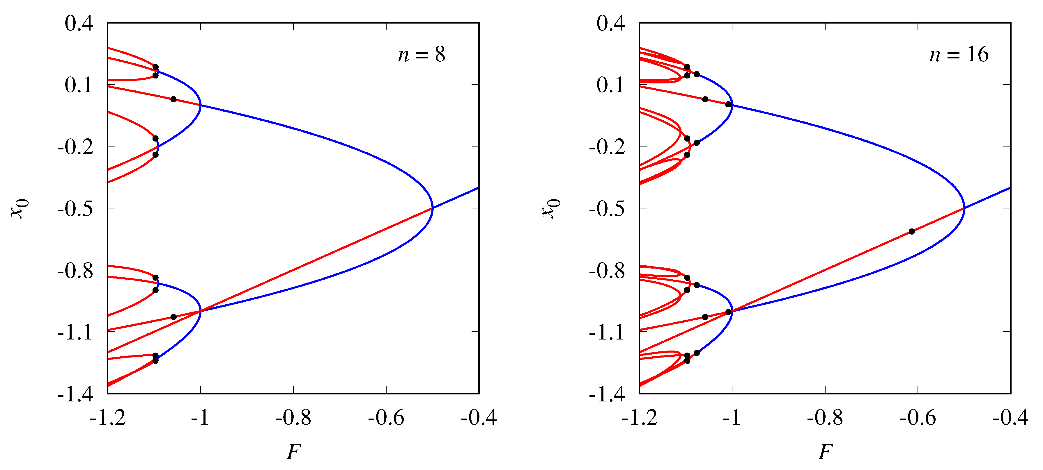
However, apart from this quantitative difference, there is also a qualitative difference. In the Lorenz-96 model with the four equilibria created at the second pitchfork bifurcation lose stability through a Hopf bifurcation before they bifurcate again through a third pitchfork bifurcation, and this leads to 8 unstable equilibria after the pitchfork cascade. For and a Hopf bifurcation only takes place after the third pitchfork bifurcation; see Figure 2. For , the scenario is again the same as for the Lorenz-96 model: now, a Hopf bifurcation occurs again after the second pitchfork bifurcation, as in the case ; see Figure 2.
3.4. The System
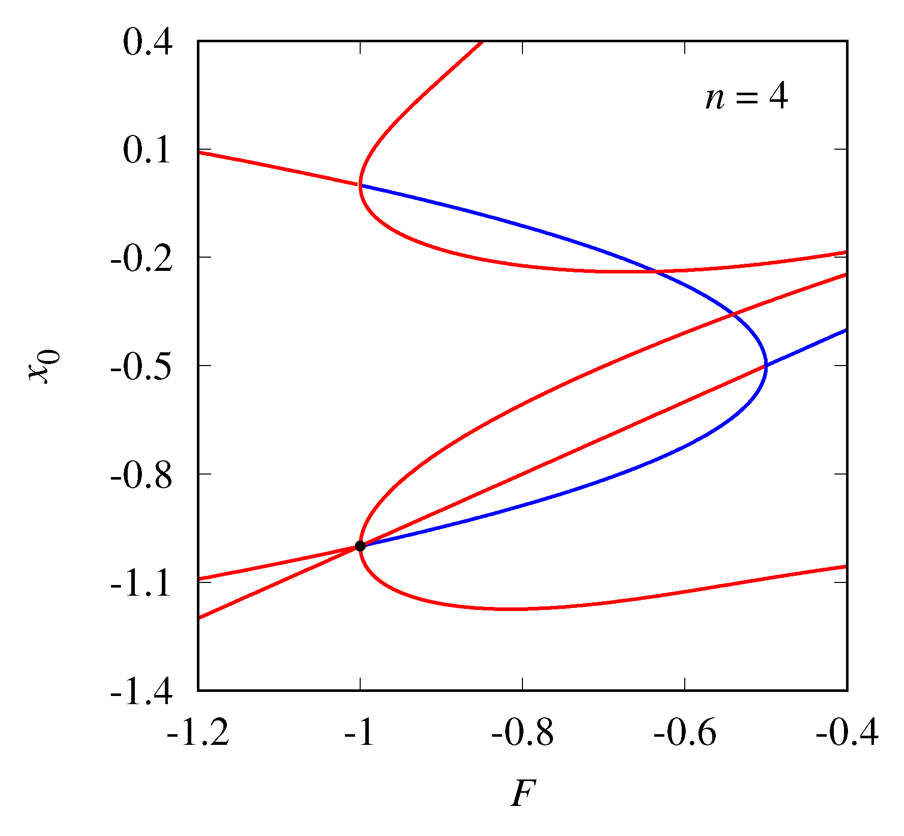
This case is very different from the Lorenz-96 model: for dimension , the second pitchfork bifurcation is subcritical. This means that the two stable equilibria that were born at the first pitchfork bifurcation for become unstable at and four new unstable equilibria come into existence for , as opposed to stable equilibria being created for ; see Figure 3. By Proposition 5, this bifurcation scenario will carry over to all dimensions n that are a multiples of four.
3.5. The System
In dimension , a succession of p pitchfork bifurcations occurs; see Table 1 for the parameter values up to . Again, the numerical results suggest that the parameter values of the pitchfork bifurcations satisfy the Feigenbaum scaling of Equation (7). However, from a qualitative point of view, this case is different from the Lorenz-96 model. Numerical computations show that, up to , the equilibria that were created in the pitchfork bifurcations do not lose stability before the last pitchfork bifurcation has occurred. Hence, there is a coexistence of stable equilibria. A Hopf bifurcation occurs only after the last pitchfork bifurcation, which leads to the coexistence of stable periodic orbits. The latter may bifurcate into chaotic attractors. Section 4 discusses some particular routes to chaos.
4. Multistability in the System
The system is of particular interest. For odd dimensions n, it follows from Lemma 1 that the equilibrium loses stability through a complex conjugate pair of eigenvalues that cross the imaginary axis. The periodic orbits that are born through this Hopf bifurcation typically bifurcate further through period doublings or Neĭmark–Sacker bifurcations. Because these scenarios are very common, they will not be discussed further in the present paper. Instead, we will focus on dimension for which a cascade of p pitchfork bifurcations is followed by a Hopf bifurcation. In this section, we discuss the fate of the coexisting stable periodic orbits that arise in this way. To that end, we will numerically compute Lyapunov exponents as a function of the parameter F to detect the relevant bifurcations. In particular, we will show that the number of coexisting attractors may become smaller than due to collisions.
4.1. Lyapunov Exponents for Coexisting Attractors
A convenient way to detect bifurcations of attractors is by computing Lyapunov exponents as a function of the continuation parameter. In systems that exhibit multistability, i.e., the coexistence of attractors, care must be taken in selecting the initial condition. However, in System (3), coexisting attractors are related by circulant shifts of coordinates. We will now explain that the Lyapunov exponents for such attractors are equal.
Denote, with C, the matrix that has the following circulant shift property:
If denotes the right-hand side of Equation (3), then for all . In particular, if is a solution of (3), then it is . If two vectors satisfy the relation , then the fact that f only has quadratic nonlinearities implies that
In particular, if satisfies the variational equation , then satisfies the variational equation . The usual algorithm for computing Lyapunov exponents consists of integrating the variational equations and applying the Gram–Schmidt procedure to the variational vectors [32,33]; see [34,35] for alternative methods. It is clear that the matrix C is unitary and, thus, preserves the Euclidean inner product. Hence, the Lyapunov exponents that are computed for the orbits and must be the same. By induction, the Lyapunov exponents will be the same for the orbits for all .
For a fixed parameter value F, we first perform a transient integration in order to obtain an initial condition on an attractor. For the attractor, we then compute the Lyapunov exponents while using the algorithm described in [32,33]. As explained above, the attractors with initial condition have the same Lyapunov exponents for all . During the computation, we also minimize the -coordinate along the attractors:
where T is the total integration time is used in our computations. If for , then the attractors with initial points and are different. In case that , we have a strong indication that the attractors with initial points and are equal. Hence, the quantities help to detect collisions of attractors. To the final point on the attractor, a small random perturbation is added, the parameter F is increased by a small step size, and the computations are repeated. The two largest Lyapunov exponents and the quantities are then plotted as a function of F. In the resulting diagram, bifurcations of attractors manifest themselves as parameter values for which a Lyapunov exponent becomes zero, and collisions of attractors manifest themselves as parameter values for which at least two of the quantities attain the same value.
4.2. Dimension
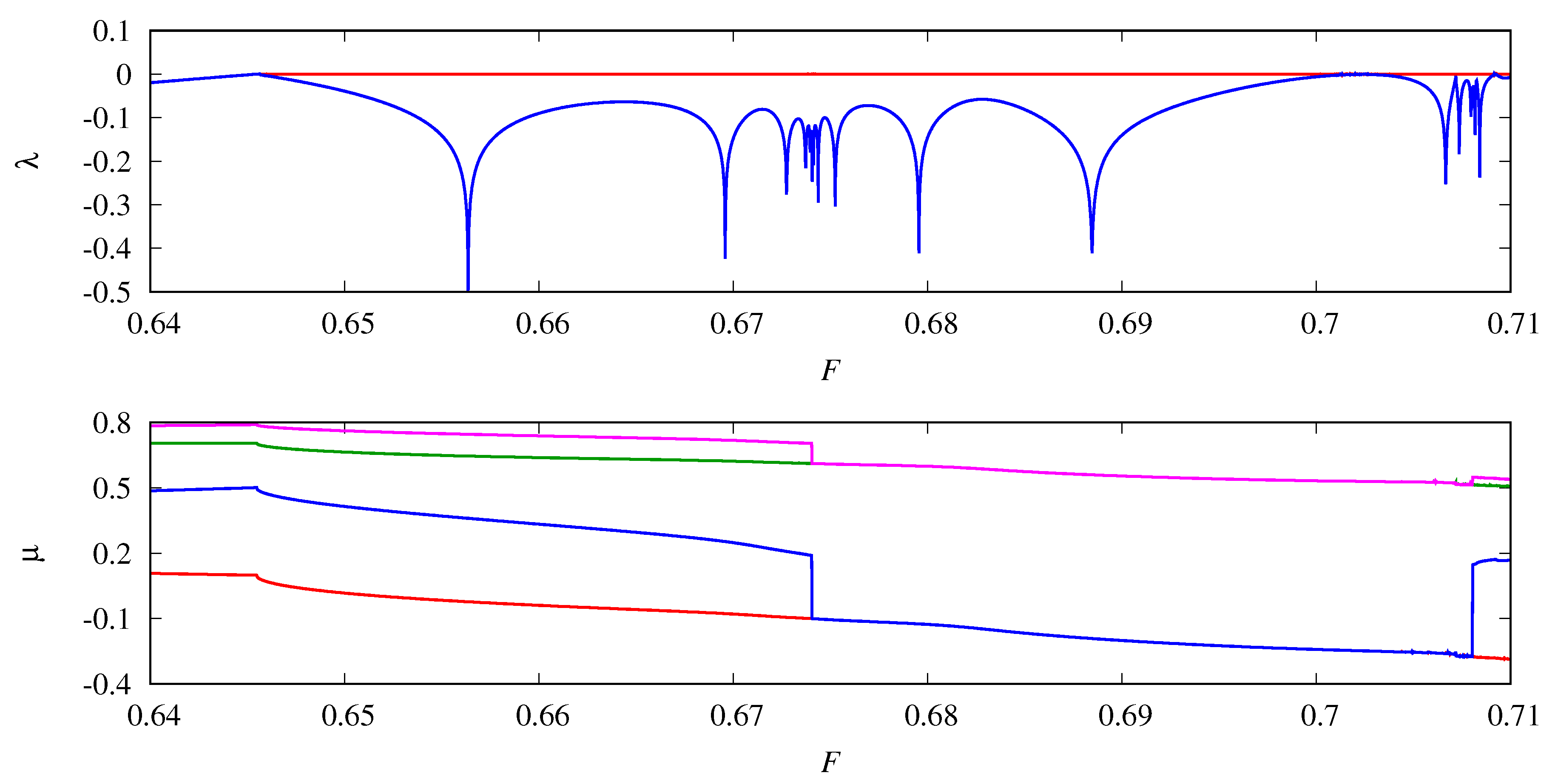
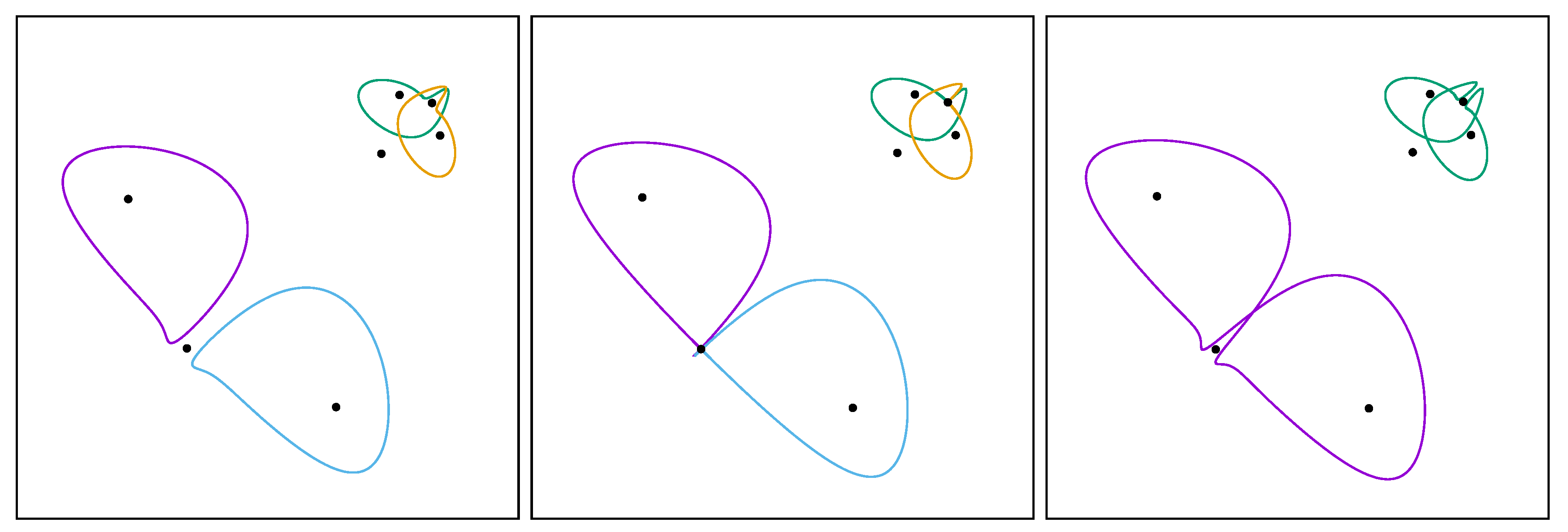
Figure 4 shows the Lyapunov diagram for dimension . After the second pitchfork bifurcation at , four stable equilibria coexist. At , these equilibria become unstable through a supercritical Hopf bifurcation, which leads to the coexistence of four stable periodic orbits; for , these orbits are shown in Figure 5 (left panel). At , one pair of periodic orbits collides with an equilibrium, while another pair of periodic orbits collides with a different equilibrium. This leads to the creation of four homoclinic orbits that form two curves in a “figure eight” configuration, see Figure 5 (middle panel). After the collision, each of the “figure eight” curves split into two coexisting stable periodic orbits, see Figure 5 (right panel). This shows how the number coexisting attractors can change due to the collision of an attractor with another invariant object.
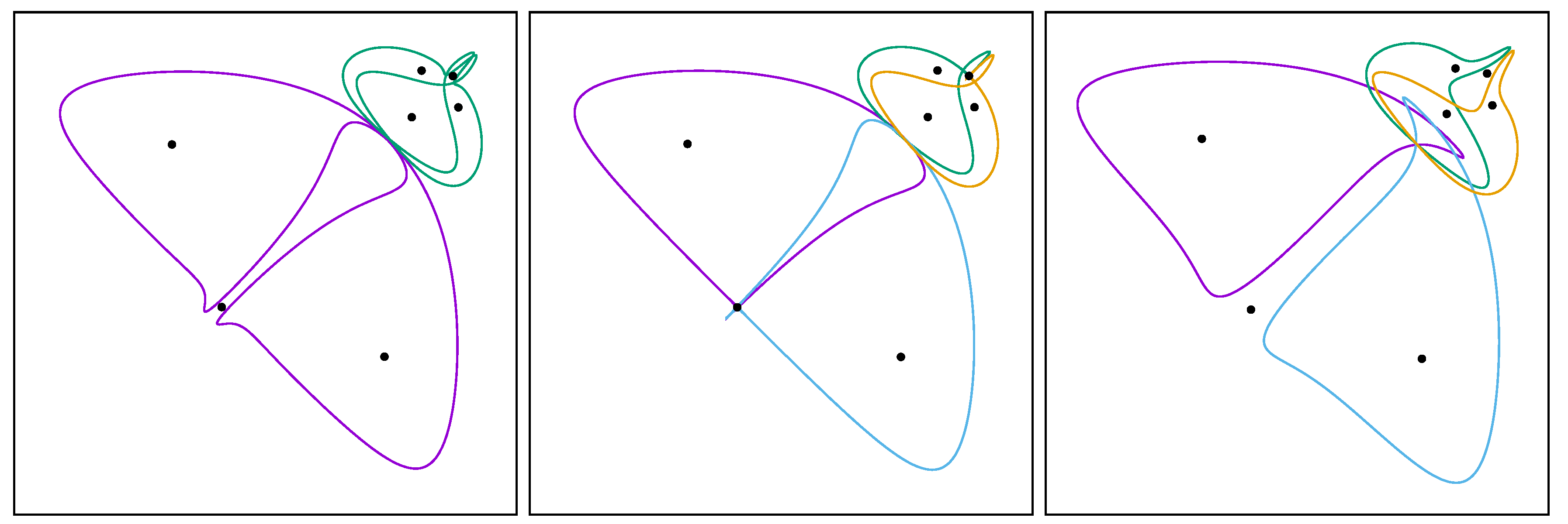
A similar scenario, as described above, can also increase the number of coexisting attractors. At , two stable periodic orbits collide with an equilibrium. This gives rise to four homoclinic orbits forming two “figure eight” curves. After the homoclinic bifurcation, there are again four coexisting stable periodic orbits, see Figure 6.
4.3. Dimension
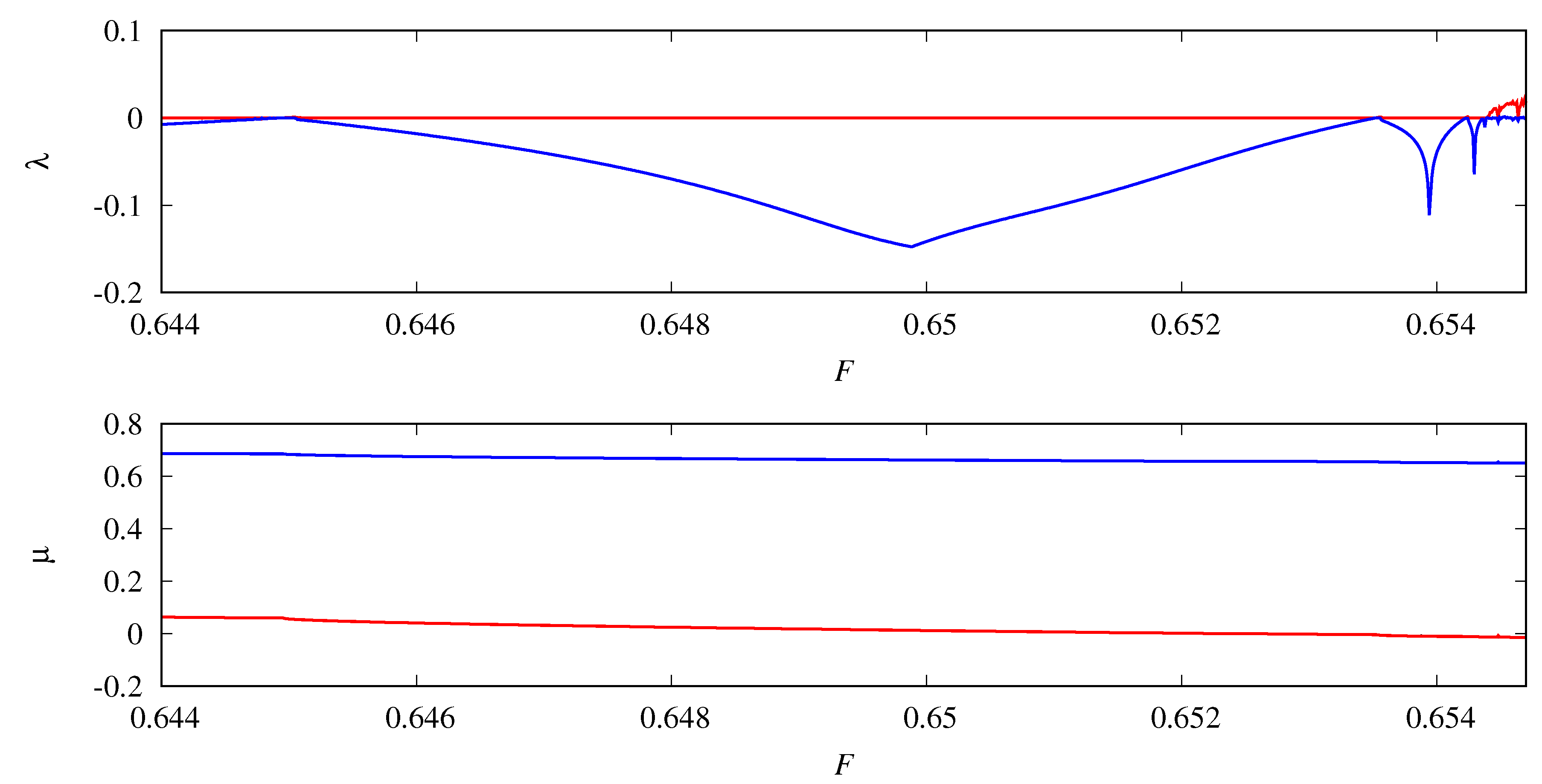
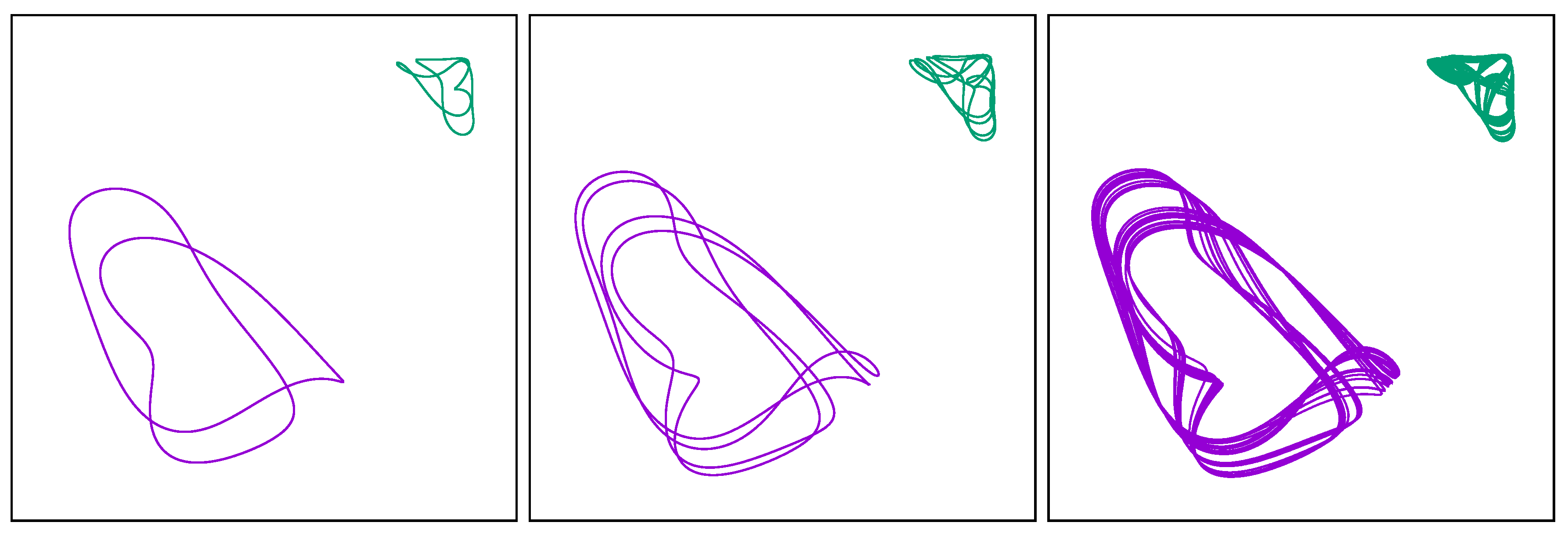
Figure 7 shows the Lyapunov diagram for dimension . Despite the dimension being larger, the bifurcation scenario is somewhat simpler in this case, since periodic orbits do not collide with equilibria, as in the case . There is only one pitchfork bifurcation at after which two stable equilibria coexist. Each of these equilibria becomes unstable through a supercritical Hopf bifurcation at , which leads to the coexistence of two stable periodic orbits. Each of these bifurcates through a period doubling cascade, which leads to the coexistence of two chaotic attractors. Figure 8 shows periodic orbits after one period doubling (), after two period doublings (), and the chaotic attractors after the cascade (). Chaotic attractors that arise after a period doubling cascade are typically observed to have a Hénon-like structure, which means that the attractors are formed by the closure of the unstable manifold of saddle periodic orbit [23,36,37].
4.4. Dimension
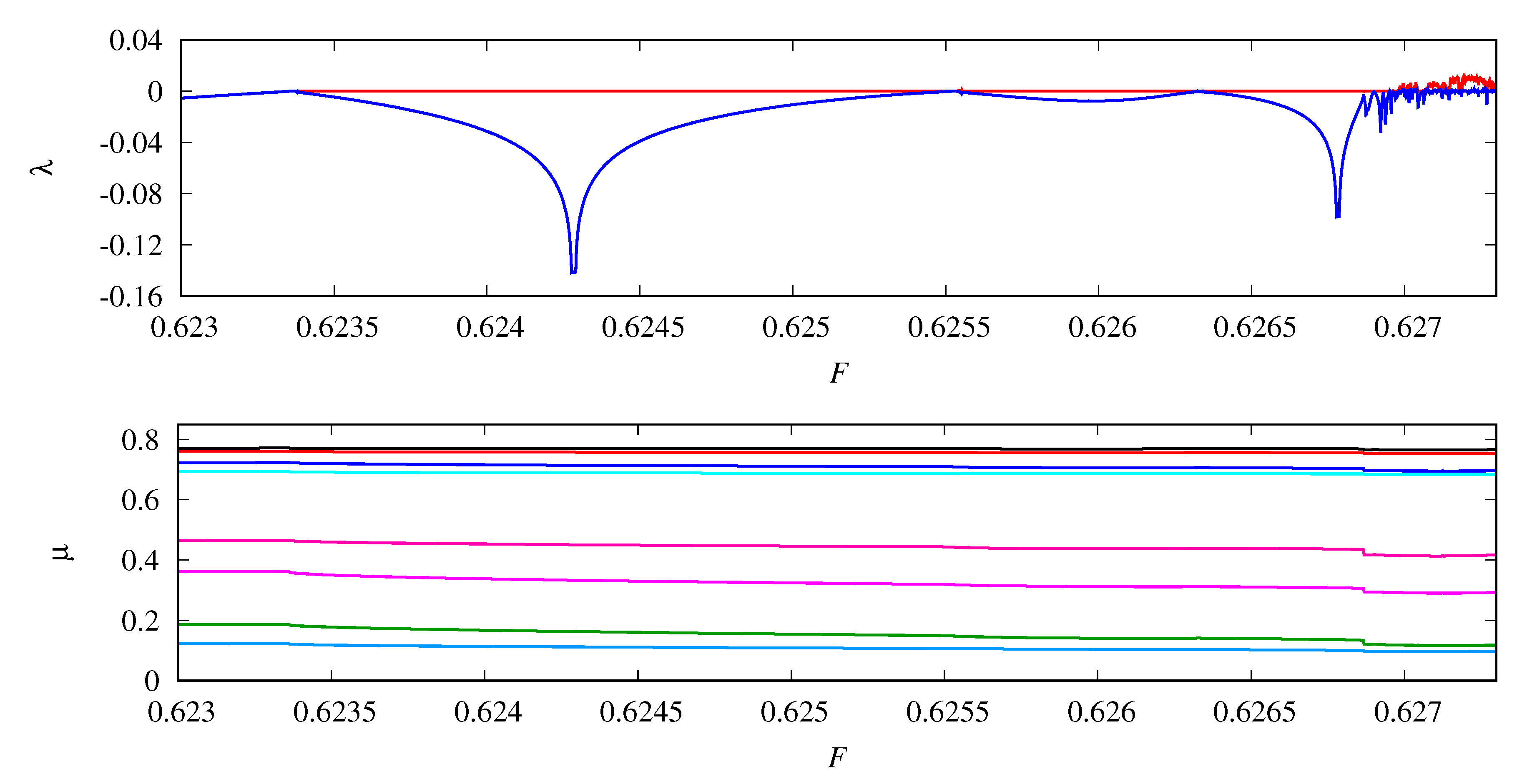
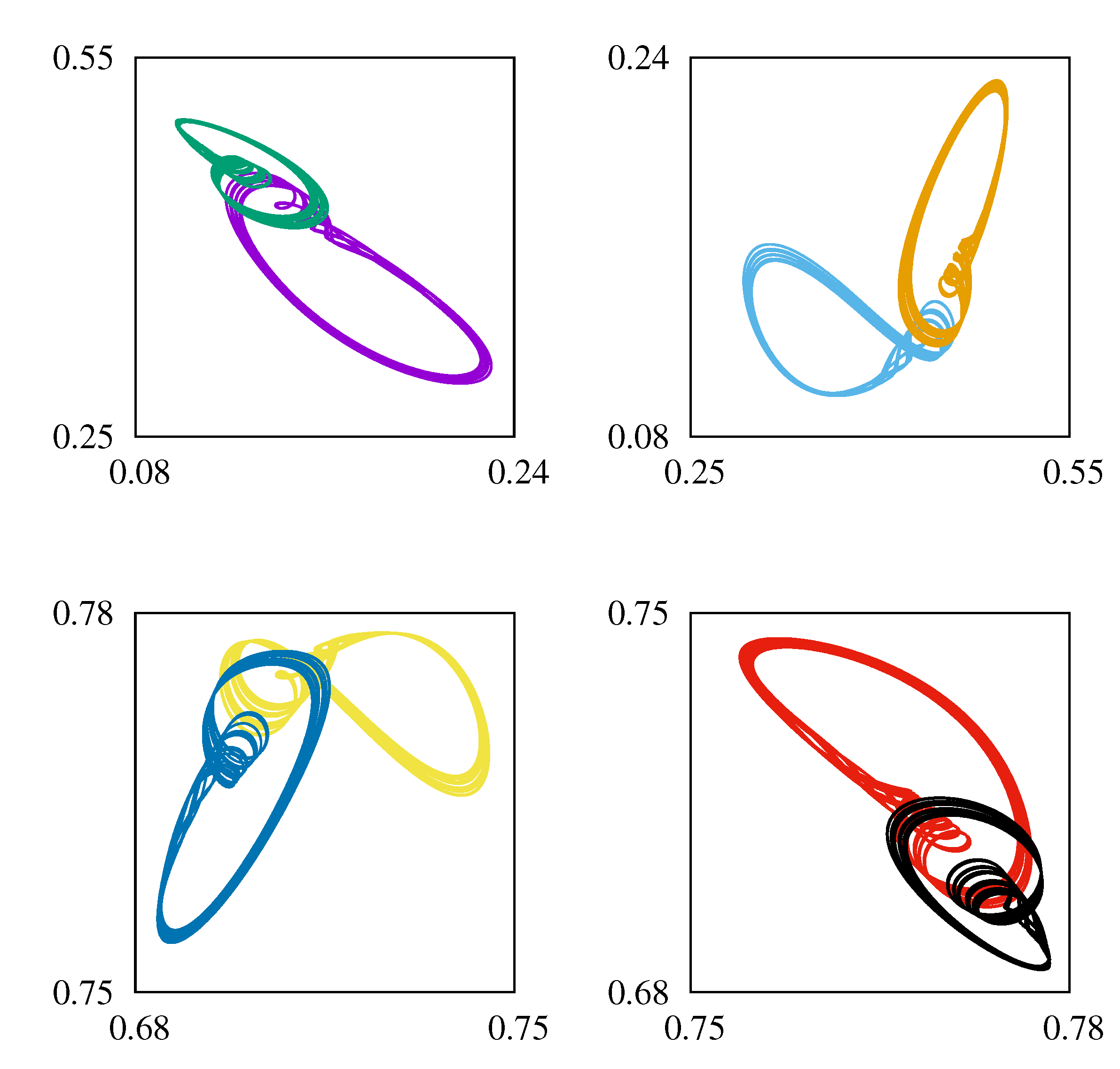
Figure 9 shows the Lyapunov diagram for dimension . After the last pitchfork bifurcation at , eight stable equilibria coexist. Each of these equilibria becomes unstable at through a supercritical Hopf bifurcation, which leads to the coexistence of eight stable periodic orbits. These periodic orbits undergo a period doubling bifurcation at and a period halving bifurcation at . At , the periodic orbits disappear through a saddle-node bifurcation. For , eight different stable periodic orbits coexist. The latter have more windings than the formerly existing periodic orbits, which suggests that the new periodic orbits already have bifurcated through a succession of period doubling bifurcations. Finally, a period doubling cascade takes place, which leads to the formation of eight coexisting chaotic attractors; for , these are plotted in Figure 10.
5. Discussion
In this paper, we have considered a family of generalized Lorenz-96 models, of which each member is parameterized by a triple . In particular, we have shown for two concrete members in this family that a finite cascade of pitchfork bifurcations takes place, just as in the original Lorenz-96 model. In particular, in the system , the equilibria remain stable up to the last pitchfork bifurcation. This is a qualitative difference with the Lorenz-96 model, in which equilibria already undergo a Hopf bifurcation after the second pitchfork bifurcation. The Hopf bifurcations of the stable equilibria lead to the coexistence of periodic attractors. Further bifurcations of the latter can result in the coexistence of chaotic attractors. The number of attractors that coexist can change due to collisions.
The results that are presented in this paper give rise to several open questions that warrant further research. The first question is whether the pitchfork cascade in the models , , and continues indefinitely when the dimension n increases. Numerical computations show the occurrence of pitchfork bifurcations up to dimension , but this does not guarantee that the pitchfork bifurcations will persist for . Indeed, in the model , the second pitchfork bifurcation becomes subcritical and the cascade comes to a halt.
How to check whether the pitchfork bifurcations persist for dimensions ? An attempt at explicitly computing all of the equilibria and their bifurcations would not be useful for at least two reasons. The first reason is that an analytical computation is simply not feasible due to the fact that the equilibria born through pitchfork bifurcations will have complicated expressions involving radicals; already after two pitchfork bifurcations, analytical expressions become unwieldy. The second reason is that an explicit computation would only provide information regarding one particular model, whereas our numerical computations suggest that properties of the pitchfork cascade are common to at least three members of the family .
Another open question is whether there exist dynamical systems with a finite-dimensional state space, in which an infinite cascade of pitchfork bifurcations occurs. Most likely, such systems cannot have only polynomial nonlinearities. Indeed, as a consequence of Bezout’s theorem, generically one expects only finitely many equilibria in such systems. Exceptions are degenerate cases, such as system , which has infinitely many equilibria for certain parameter values. However, for systems with transcendental nonlinearities, the situation might be different. These open questions will have to be addressed in future research.
It is an intriguing numerical observation that the parameter values of the pitchfork bifurcations that are described above satisfy the Feigenbaum scaling in Equation (7). The latter scaling was originally discovered in period doubling cascades of periodic points in unimodal maps [38,39]. A key feature is its universal nature, which means that the scaling holds for an entire class of unimodal maps possesing a quadratic maximum, rather than just one particular map. Lanford [40] and Eckmann and Wittwer [41] provided computer assisted proofs of the Feigenbaum conjectures. A computer-free proof was given by Lyubich [42]. Briggs [43,44] carried out high-precision computations of the Feigenbaum constants.
The fact that the Feigenbaum scaling for the pitchfork bifurcations occurs in at least three different members of the family suggests that it might be a universal property within a suitably chosen class of systems. However, it is not clear a priori how this could be analytically proven. Proof strategies, as in [40,41,42], are not applicable in the context of System (3) because of several conceptual differences. Firstly, (3) is not a map but a differential equation. Secondly, the pitchfork cascade in System (3) is finite and the dimension needs to increase in order to observe a longer cascade. If one is interested in universality, then the first step is to identify an appropriate class of systems for which a universal result can be conjectured. Perhaps pitchfork cascades can occur in systems that are different from Equation (3) provided a sufficient amount of symmetry is present. However, to the best of our knowledge, examples of such systems are unknown to us.
Finally, the results that are presented in this paper also illustrate the important point that bifurcation scenarios in the models strongly depend on divisibility properties of the dimension n. The relevance of this phenomenon extends beyond the context of this paper. As an example, for discretisations of Burgers’ equation, it has been observed that, for odd degrees of freedom, the dynamics are confined to an invariant subspace, whereas, for even degrees of freedom, this is not the case. In turn, this has an effect on the bifurcation diagrams that one observes in this model [45]. Similar phenomena can be expected in the discretisations of partial differential equations, in which periodic boundary conditions lead to circulant symmetries.
Author Contributions
Conceptualization, A.E.S.; methodology, A.F.G.P. and A.E.S.; software, A.F.G.P. and A.E.S.; formal analysis, A.F.G.P. and A.E.S.; writing—original draft preparation, A.E.S.; writing—review and editing, A.F.G.P.; visualization, A.F.G.P. and A.E.S.; supervision, A.E.S.; All authors have read and agreed to the published version of the manuscript.
Funding
This research received no external funding.
Conflicts of Interest
The authors declare no conflict of interest.
References
- Lorenz, E.N. Predictability—A problem partly solved. In Predictability of Weather and Climate; Palmer, T.N., Hagedorn, R., Eds.; Cambridge University Press: Cambridge, UK, 2006; pp. 40–58. [Google Scholar]
- Lorenz, E. Deterministic nonperiodic flow. J. Atmos. Sci. 1963, 20, 130–141. [Google Scholar] [CrossRef] [Green Version]
- Lorenz, E. Irregularity: A fundamental property of the atmosphere. Tellus 1984, 36A, 98–110. [Google Scholar] [CrossRef]
- Van Veen, L. Baroclinic flow and the Lorenz-84 model. Int. J. Bifurc. Chaos 2003, 13, 2117–2139. [Google Scholar] [CrossRef] [Green Version]
- Viana, M. What’s new on Lorenz strange attractors? Math. Intell. 2000, 22, 6–19. [Google Scholar] [CrossRef]
- Basnarkov, L.; Kocarev, L. Forecast improvement in Lorenz 96 system. Nonlinear Process. Geophys. 2012, 19, 569–575. [Google Scholar] [CrossRef] [Green Version]
- Danforth, C.; Yorke, J. Making forecasts for chaotic physical processes. Phys. Rev. Lett. 2006, 96, 144102. [Google Scholar] [CrossRef] [Green Version]
- Orrell, D. Role of the metric in forecast error growth: How chaotic is the weather? Tellus A 2002, 54, 350–362. [Google Scholar] [CrossRef]
- Orrell, D.; Smith, L.; Barkmeijer, J.; Palmer, T. Model error in weather forecasting. Nonlinear Process. Geophys. 2001, 8, 357–371. [Google Scholar] [CrossRef] [Green Version]
- Haven, K.; Majda, A.; Abramov, R. Quantifying predictability through information theory: Small sample estimation in a non-Gaussian framework. J. Comput. Phys. 2005, 206, 334–362. [Google Scholar] [CrossRef]
- Sterk, A.; Holland, M.; Rabassa, P.; Broer, H.; Vitolo, R. Predictability of extreme values in geophysical models. Nonlinear Process. Geophys. 2012, 19, 529–539. [Google Scholar] [CrossRef] [Green Version]
- Sterk, A.; Van Kekem, D. Predictability of extreme waves in the Lorenz-96 model near intermittency and quasi-periodicity. Complexity 2017, 2017, 9419024. [Google Scholar] [CrossRef]
- Hallerberg, S.; Pazó, D.; López, J.; Rodríguez, M. Logarithmic bred vectors in spatiotemporal chaos: Structure and growth. Phys. Rev. E 2010, 81, 066204. [Google Scholar] [CrossRef] [PubMed] [Green Version]
- Karimi, A.; Paul, M. Extensive chaos in the Lorenz-96 model. Chaos Interdiscip. J. Nonlinear Sci. 2010, 20, 043105. [Google Scholar] [CrossRef] [PubMed] [Green Version]
- Orrell, D.; Smith, L. Visualising bifurcations in high dimensional systems: The spectral bifurcation diagram. Int. J. Bifurc. Chaos 2003, 13, 3015–3027. [Google Scholar] [CrossRef] [Green Version]
- Pazó, D.; Szendro, I.; López, J.; Rodríguez, M. Structure of characteristic Lyapunov vectors in spatiotemporal chaos. Phys. Rev. E 2008, 78, 016209. [Google Scholar] [CrossRef] [Green Version]
- De Leeuw, B.; Dubinkina, S.; Frank, J.; Steyer, A.; Tu, X.; Van Vleck, E. Projected shadowing-based data assimilation. SIAM J. Appl. Dyn. Syst. 2018, 17, 2446–2477. [Google Scholar] [CrossRef] [Green Version]
- Ott, E.; Hunt, B.; Szunyogh, I.; Zimin, A.; Kostelich, E.; Corazza, M.; Kalnay, E.; Patil, D.; Yorke, J. A local ensemble Kalman filter for atmospheric data assimilation. Tellus 2004, 56A, 415–428. [Google Scholar] [CrossRef]
- Stappers, R.; Barkmeijer, J. Optimal linearization trajectories for tangent linear models. Q. J. R. Meteorol. Soc. 2012, 138, 170–184. [Google Scholar] [CrossRef] [Green Version]
- Trevisan, A.; Palatella, L. On the Kalman filter error covariance collapse into the unstable subspace. Nonlinear Process. Geophys. 2011, 18, 243–250. [Google Scholar] [CrossRef]
- Kerin, J.; Engler, H. On the Lorenz ’96 model and some generalizations. arXiv 2020, arXiv:2005.07767. [Google Scholar]
- Vissio, G.; Lucarini, V. Mechanics and thermodynamics of a new minimal model of the atmosphere. Eur. Phys. J. Plus 2020, 135, 807. [Google Scholar] [CrossRef]
- Van Kekem, D.; Sterk, A. Travelling waves and their bifurcations in the Lorenz-96 model. Phys. D Nonlinear Phenom. 2018, 367, 38–60. [Google Scholar] [CrossRef] [Green Version]
- Van Kekem, D.; Sterk, A. Wave propagation in the Lorenz-96 model. Nonlinear Process. Geophys. 2018, 25, 301–314. [Google Scholar] [CrossRef] [Green Version]
- Van Kekem, D.; Sterk, A. Symmetries in the Lorenz-96 model. Int. J. Bifurc. Chaos 2019, 29, 1950008. [Google Scholar] [CrossRef] [Green Version]
- Lorenz, E. Attractor sets and quasi-geostrophic equilibrium. J. Atmos. Sci. 1980, 37, 1685–1699. [Google Scholar] [CrossRef]
- Sterk, A.; Vitolo, R.; Broer, H.; Simó, C.; Dijkstra, H. New nonlinear mechanisms of midlatitude atmospheric low-frequency variability. Phys. D Nonlinear Phenom. 2010, 239, 702–718. [Google Scholar] [CrossRef] [Green Version]
- Gray, R. Toeplitz and circulant matrices: A review. Found. Trends Commun. Inf. Theory 2006, 2, 155–239. [Google Scholar] [CrossRef]
- Kuznetsov, Y.A. Elements of Applied Bifurcation Theory, 3rd ed.; Springer: New York, NY, USA, 2004. [Google Scholar]
- Van Kekem, D. Dynamics of the Lorenz-96 model: Bifurcations, symmetries and waves. Ph.D. Thesis, University of Groningen, Groningen, The Netherlands, 2018. [Google Scholar]
- Doedel, E.; Oldeman, B. AUTO–07p: Continuation and Bifurcation Software for Ordinary Differential Equations. Available online: https://www.macs.hw.ac.uk/~gabriel/auto07/auto.html (accessed on 9 December 2020).
- Benettin, G.; Galgani, L.; Giorgilli, A.; Strelcyn, J.M. Lyapunov characteristic exponents for smooth dynamical systems and for Hamiltonian systems; A method for computing all of them. Part 1: Theory. Meccanica 1980, 15, 9–20. [Google Scholar] [CrossRef]
- Benettin, G.; Galgani, L.; Giorgilli, A.; Strelcyn, J.M. Lyapunov characteristic exponents for smooth dynamical systems and for Hamiltonian systems; A method for computing all of them. Part 2: Numerical application. Meccanica 1980, 15, 21–30. [Google Scholar] [CrossRef]
- Dieci, L. Jacobian Free Computation of Lyapunov Exponents. J. Dyn. Differ. Equ. 2002, 14, 697–717. [Google Scholar] [CrossRef]
- Dieci, L.; Russel, R.; van Vleck, E. On the Computation of Lyapunov Exponents for Continuous Dynamical Systems. SIAM J. Numer. Anal. 1997, 34, 402–423. [Google Scholar] [CrossRef] [Green Version]
- Broer, H.; Dijkstra, H.; Simó, C.; Sterk, A.; Vitolo, R. The dynamics of a low-order model for the Atlantic Multidecadal Oscillation. Discrete Contin. Dyn. Syst. B 2011, 16, 73–107. [Google Scholar] [CrossRef]
- Ghane, H.; Sterk, A.; Waalkens, H. Chaotic dynamics from a pseudo-linear system. IMA J. Math. Control Inf. 2019. [Google Scholar] [CrossRef]
- Feigenbaum, M. Quantitative universality for a class of nonlinear transformations. J. Stat. Phys. 1978, 19, 25–52. [Google Scholar] [CrossRef]
- Feigenbaum, M. The universal metric properties of nonlinear transformations. J. Stat. Phys. 1979, 21, 669–706. [Google Scholar] [CrossRef]
- Lanford, O., III. A computer-assisted proof of the Feigenbaum conjectures. Bull. Am. Math. Soc. 1982, 6, 427–434. [Google Scholar] [CrossRef] [Green Version]
- Eckmann, J.P.; Wittwer, P. A complete proof of the Feigenbaum conjectures. J. Stat. Phys. 1987, 46, 455–475. [Google Scholar] [CrossRef]
- Lyubich, M. Feigenbaum–Coullet–Tresser universality and Milnor’s hairiness conjecture. Ann. Math. 1999, 149, 319–420. [Google Scholar] [CrossRef]
- Briggs, K. A precise calculation of the Feigenbaum constants. Math. Comput. 1991, 57, 435–439. [Google Scholar] [CrossRef]
- Briggs, K. Feigenbaum Scaling in Discrete Dynamical Systems. Ph.D. Thesis, University of Melbourne, Melbourne, Australia, 1997. [Google Scholar]
- Basto, M.; Semiao, V.; Calheiros, F. Dynamics in spectral solutions of Burgers equation. J. Comput. Appl. Math. 2006, 205, 296–304. [Google Scholar] [CrossRef] [Green Version]
Figure 1.
Numerical estimates of the quantity plotted as a function of n for seven different choices of the triple . Note that a logarithmic scale is used for both axes. The two dashed lines represent the curves and , which suggest that with .
Figure 1.
Numerical estimates of the quantity plotted as a function of n for seven different choices of the triple . Note that a logarithmic scale is used for both axes. The two dashed lines represent the curves and , which suggest that with .

Figure 2.
Bifurcation diagrams for the system with and . For dimension a Hopf bifurcation (marked with a bullet) destabilizes the equilibria after the last pitchfork bifurcation, whereas, for dimension , the Hopf bifurcation already occurs before the last pitchfork bifurcation.
Figure 2.
Bifurcation diagrams for the system with and . For dimension a Hopf bifurcation (marked with a bullet) destabilizes the equilibria after the last pitchfork bifurcation, whereas, for dimension , the Hopf bifurcation already occurs before the last pitchfork bifurcation.

Figure 3.
Bifurcation diagram for system with . The equilibrium becomes unstable through a supercritical pitchfork bifurcation at and the two newly created branches bifurcate through a subcritical pitchfork bifurcation at . The bullet marks a Hopf bifurcation of at .
Figure 3.
Bifurcation diagram for system with . The equilibrium becomes unstable through a supercritical pitchfork bifurcation at and the two newly created branches bifurcate through a subcritical pitchfork bifurcation at . The bullet marks a Hopf bifurcation of at .

Figure 4.
Top panel: the two largest Lyapunov exponents plotted as a function of the parameter F for the system for dimension . Bottom panel: the quantities , as defined in Equation (8) plotted as a function of F.
Figure 4.
Top panel: the two largest Lyapunov exponents plotted as a function of the parameter F for the system for dimension . Bottom panel: the quantities , as defined in Equation (8) plotted as a function of F.

Figure 5.
Collision of two pairs of periodic orbits with an equilibrium (middle); the equilibria are marked by a bullet. Before the collision (left), four periodic stable periodic orbits coexist. After the collision (right), only two stable periodic orbits coexist. Hence, the collision of periodic orbits with an equilibrium reduces the number of coexisting attractors. All panels represent the square in the -plane. The used parameter values are: (left), (middle), and (right).

Figure 6.
Similar to Figure 5, but now the collision of periodic orbits with an equilibrium increases the number of coexisting attractors; the equilibria are marked by a bullet. All panels represent the square in the -plane. The used parameter values are: (left), (middle), and (right).
Figure 6.
Similar to Figure 5, but now the collision of periodic orbits with an equilibrium increases the number of coexisting attractors; the equilibria are marked by a bullet. All panels represent the square in the -plane. The used parameter values are: (left), (middle), and (right).

Figure 7.
As Figure 4, but for dimension . Period doubling bifurcations take place for parameter values where the second Lyapunov exponent equals zero. Observe that the number of coexisting attractors remains the same across this range of parameters.
Figure 7.
As Figure 4, but for dimension . Period doubling bifurcations take place for parameter values where the second Lyapunov exponent equals zero. Observe that the number of coexisting attractors remains the same across this range of parameters.

Figure 8.
Period doubled versions of two coexisting periodic orbits (left and middle) and the coexistence of two chaotic attractors after a full cascade (right). All of the panels represent the square in the -plane. The used parameter values are: (left), (middle), and (right).
Figure 8.
Period doubled versions of two coexisting periodic orbits (left and middle) and the coexistence of two chaotic attractors after a full cascade (right). All of the panels represent the square in the -plane. The used parameter values are: (left), (middle), and (right).

Figure 9.
As Figure 4, but for dimension .
Figure 9.
As Figure 4, but for dimension .

Figure 10.
Coexistence of eight chaotic attractors. All of the panels represent a square in the -plane, but, for visual clarity, pairs of attractors are plotted in different windows. The parameter value is .
Figure 10.
Coexistence of eight chaotic attractors. All of the panels represent a square in the -plane, but, for visual clarity, pairs of attractors are plotted in different windows. The parameter value is .


Table 1.
Numerically computed parameter values for which a pitchfork bifurcation takes place in the system with dimension for . Note that is the original Lorenz-96 model. In addition, the ratio is listed, except for the system , in which case the second pitchfork bifurcation is subcritical and the cascade terminates. See the main text for explanations.
| 1 | |||||||
| 2 | |||||||
| 3 | |||||||
| 4 | |||||||
| 5 | |||||||
| 6 | |||||||
| 7 | |||||||
| 8 | |||||||
| 9 | |||||||
Publisher’s Note: MDPI stays neutral with regard to jurisdictional claims in published maps and institutional affiliations. |
© 2020 by the authors. Licensee MDPI, Basel, Switzerland. This article is an open access article distributed under the terms and conditions of the Creative Commons Attribution (CC BY) license (http://creativecommons.org/licenses/by/4.0/).
Share and Cite
MDPI and ACS Style
Pelzer, A.F.G.; Sterk, A.E. Finite Cascades of Pitchfork Bifurcations and Multistability in Generalized Lorenz-96 Models. Math. Comput. Appl. 2020, 25, 78. https://0-doi-org.brum.beds.ac.uk/10.3390/mca25040078
AMA Style
Pelzer AFG, Sterk AE. Finite Cascades of Pitchfork Bifurcations and Multistability in Generalized Lorenz-96 Models. Mathematical and Computational Applications. 2020; 25(4):78. https://0-doi-org.brum.beds.ac.uk/10.3390/mca25040078
Chicago/Turabian StylePelzer, Anouk F. G., and Alef E. Sterk. 2020. "Finite Cascades of Pitchfork Bifurcations and Multistability in Generalized Lorenz-96 Models" Mathematical and Computational Applications 25, no. 4: 78. https://0-doi-org.brum.beds.ac.uk/10.3390/mca25040078