Finite Element Analysis of Laminar Heat Transfer within an Axial-Flux Permanent Magnet Machine


Abstract
:1. Introduction
1.1. Flow Characteristics
1.2. Thermal Characteristics
1.3. Research Objective
2. Flow Model
2.1. Strong Form
2.2. Mixed Variational Form
2.2.1. Weakly Imposed Dirichlet Boundary Condition
2.2.2. Directional Do-Nothing Boundary Condition
2.3. Validation
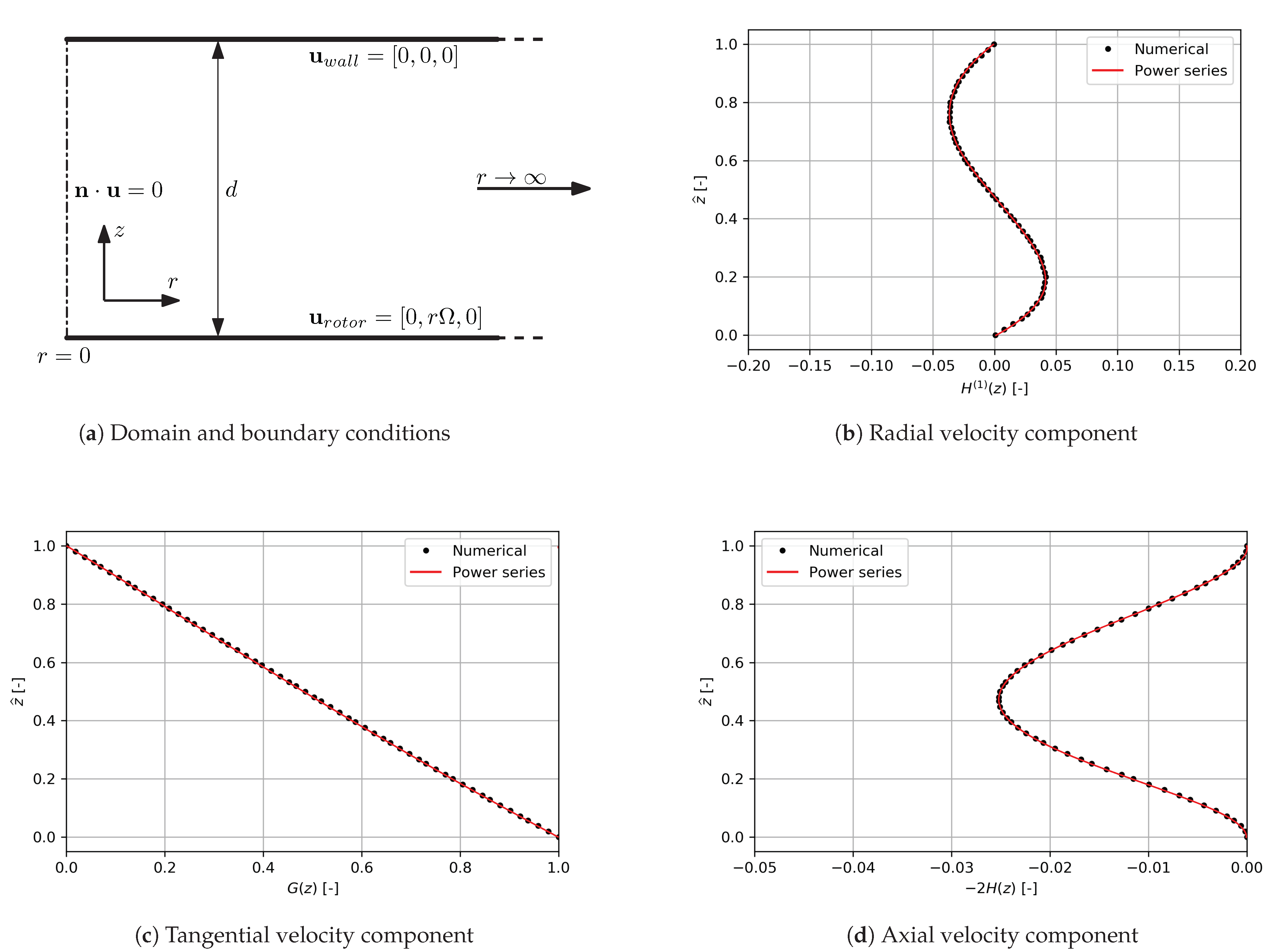
2.3.1. Enclosed Rotating Disk
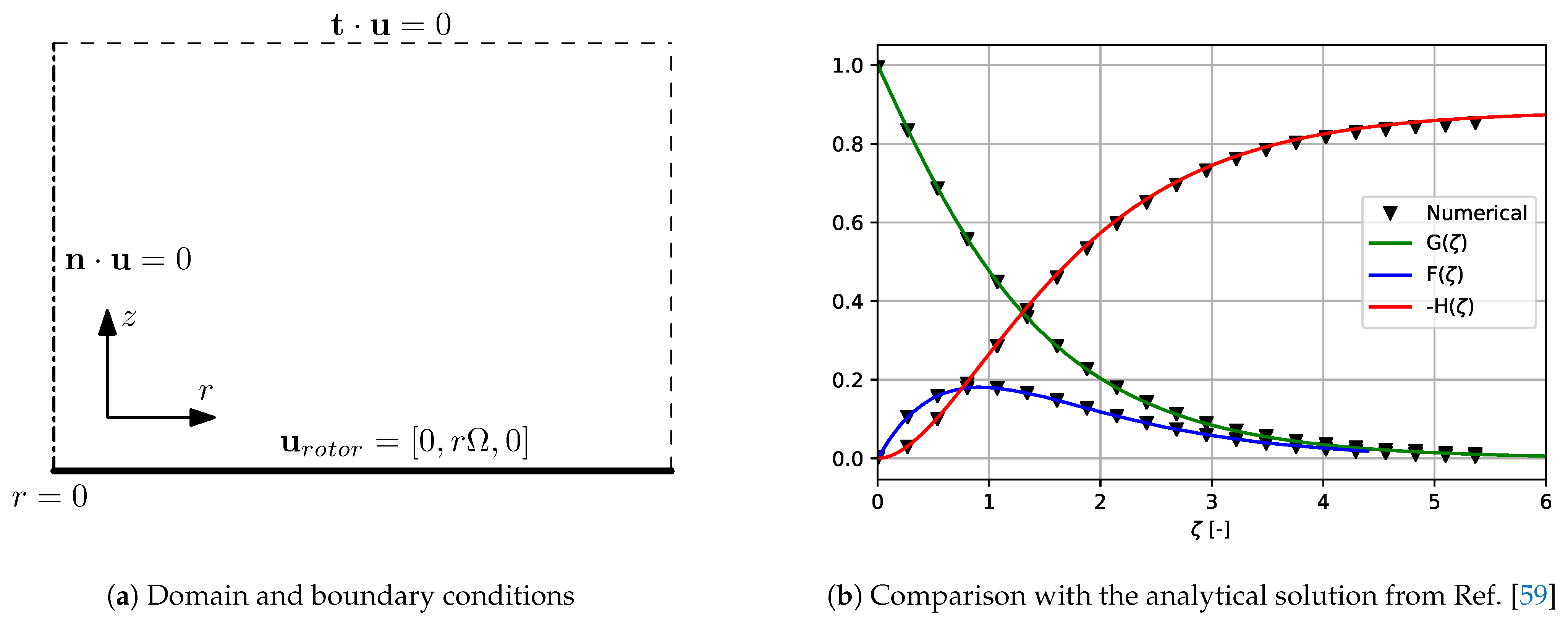
2.3.2. Von Kármán Swirling Flow
2.3.3. Infinite Rotor-Stator Configuration
3. Thermal Model
3.1. Strong Form
3.2. Variational Form
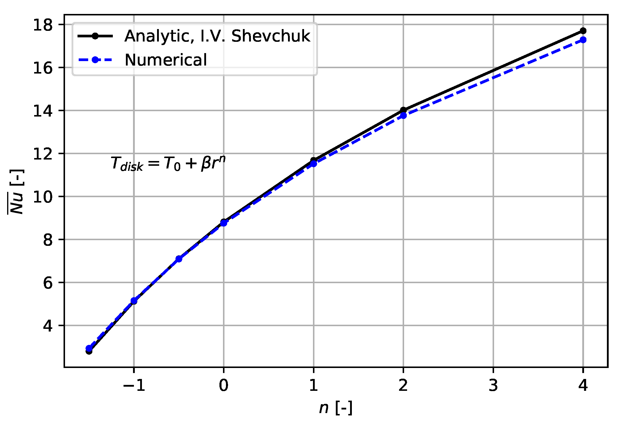
3.3. Nusselt Number
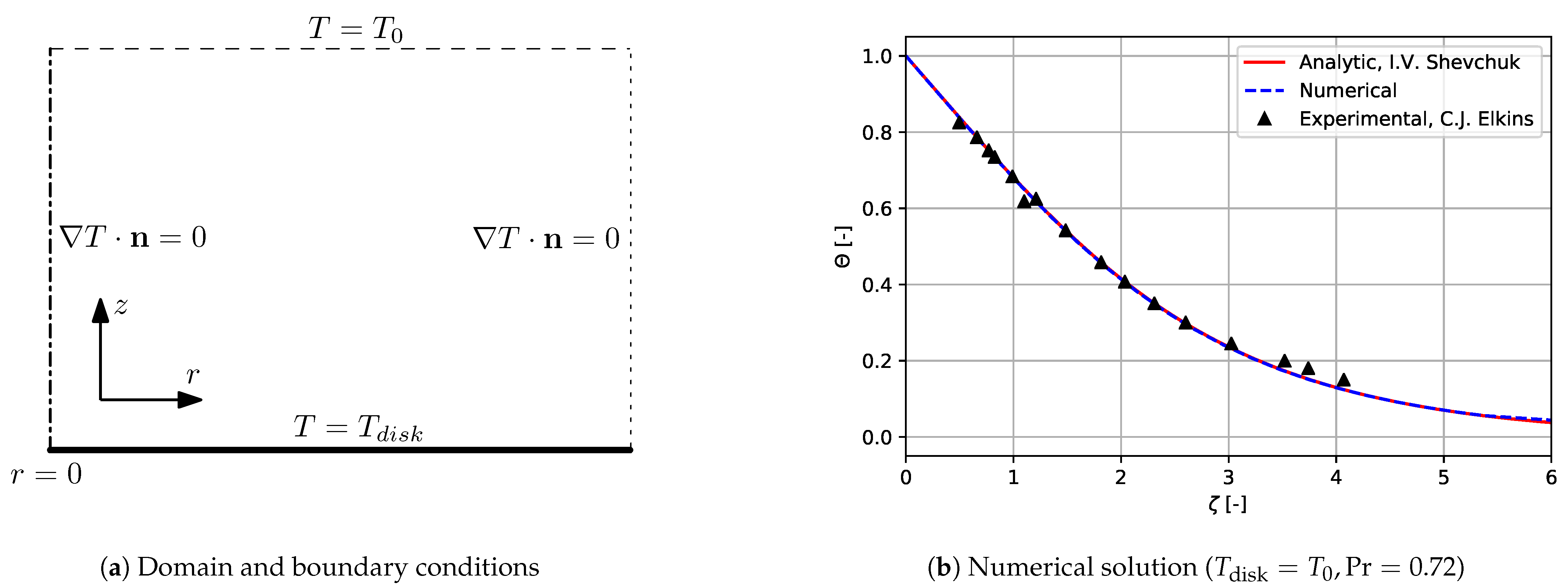
3.4. Validation
4. AFPM Simulation Setup
4.1. Numerical Domain and Mesh
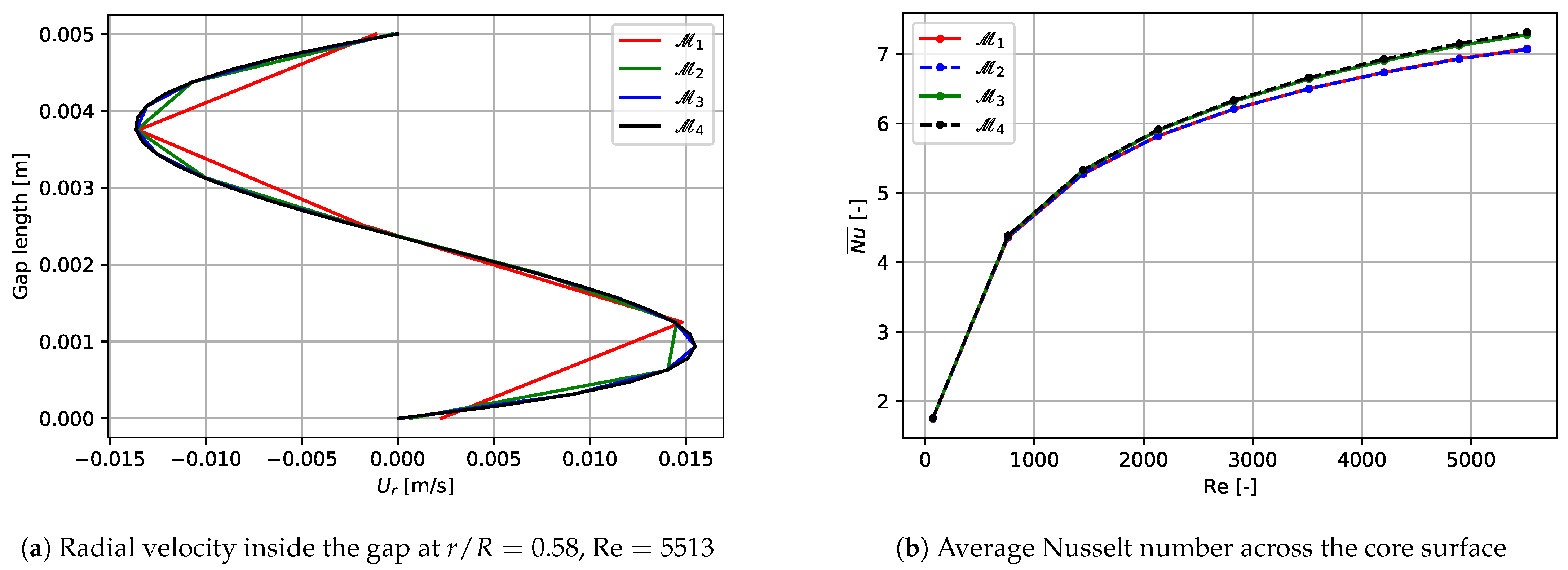
4.2. Mesh Convergence
5. AFPM Design Analyses
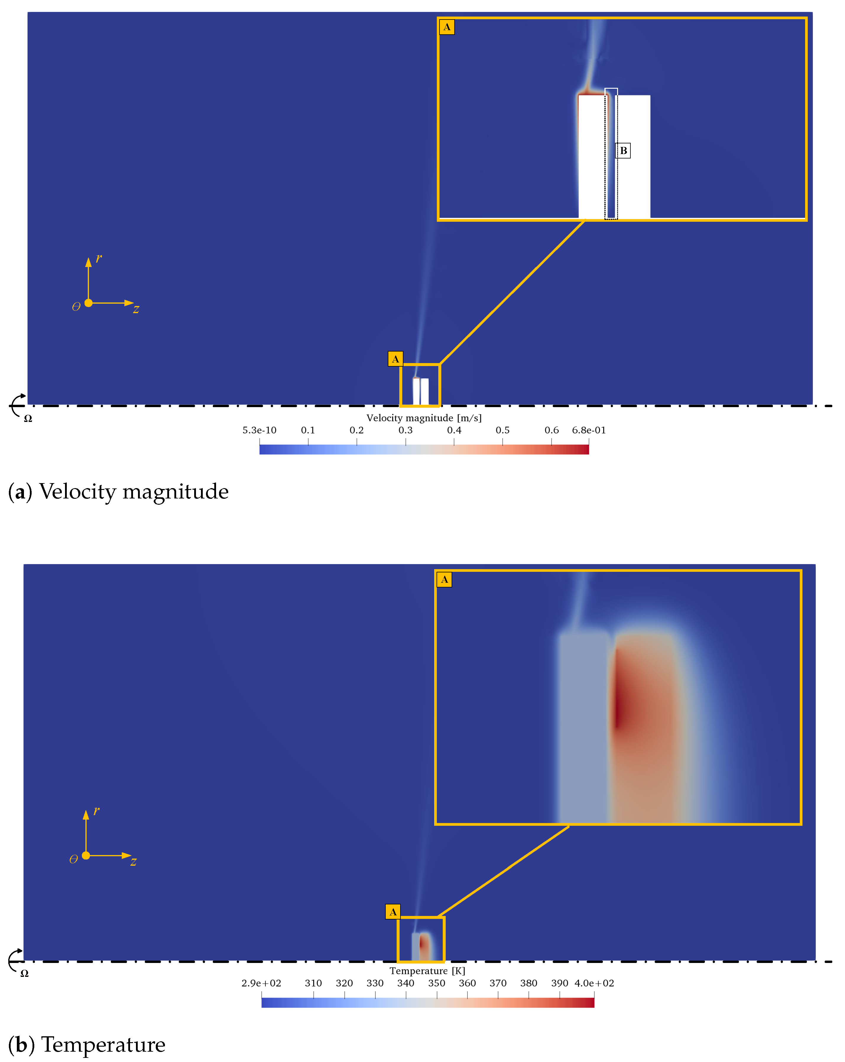
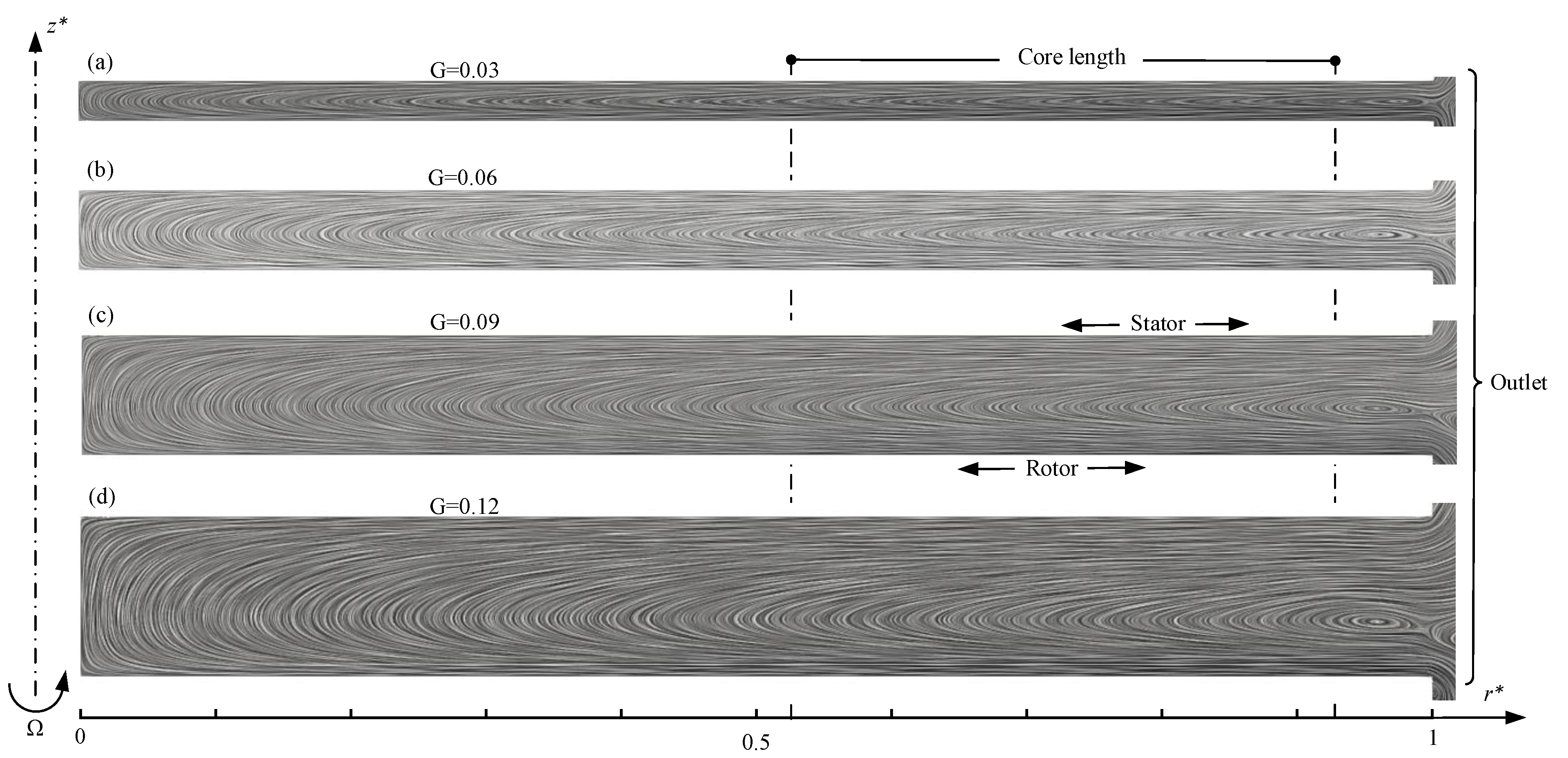
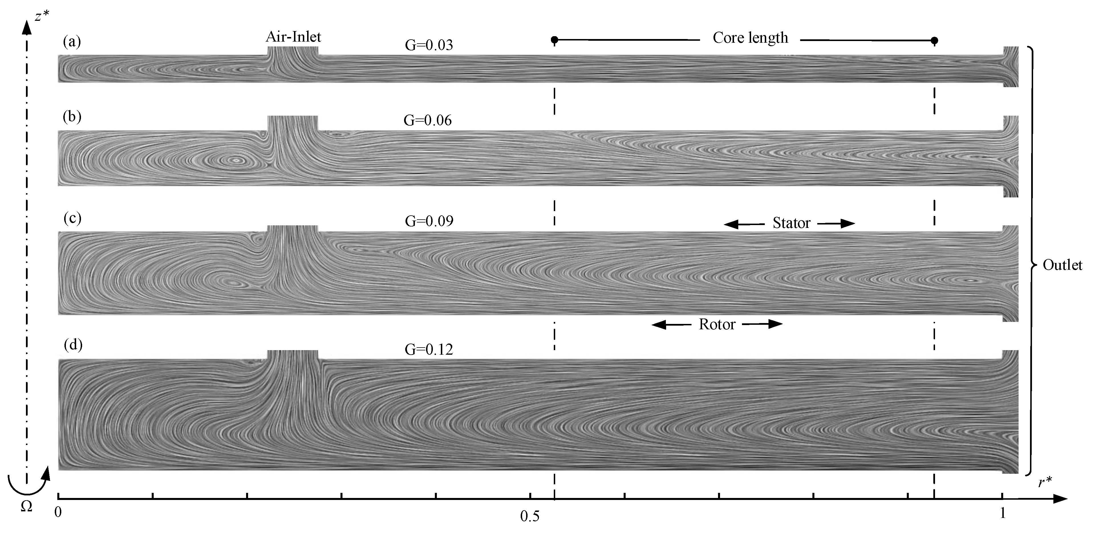
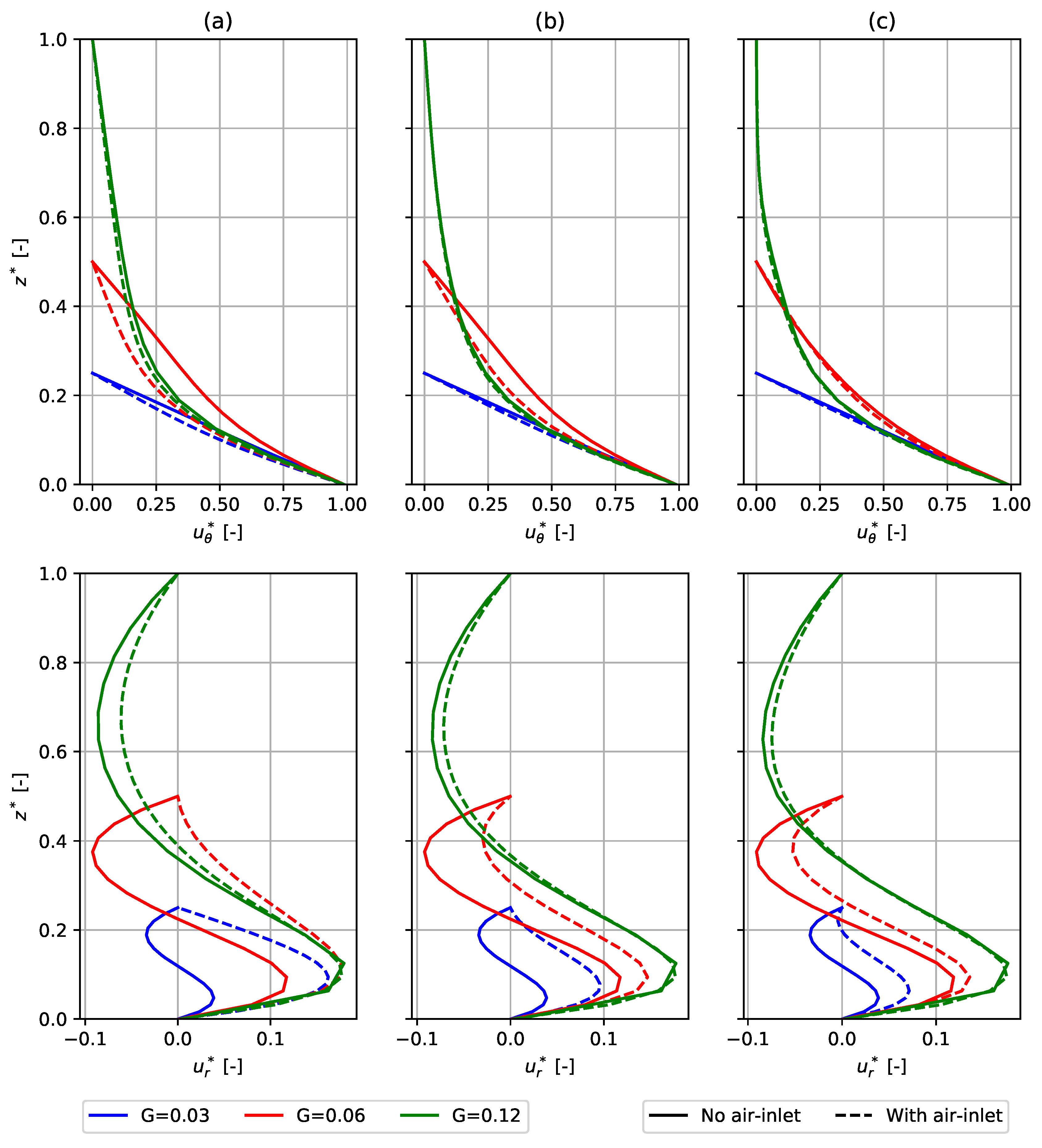
5.1. Flow Field
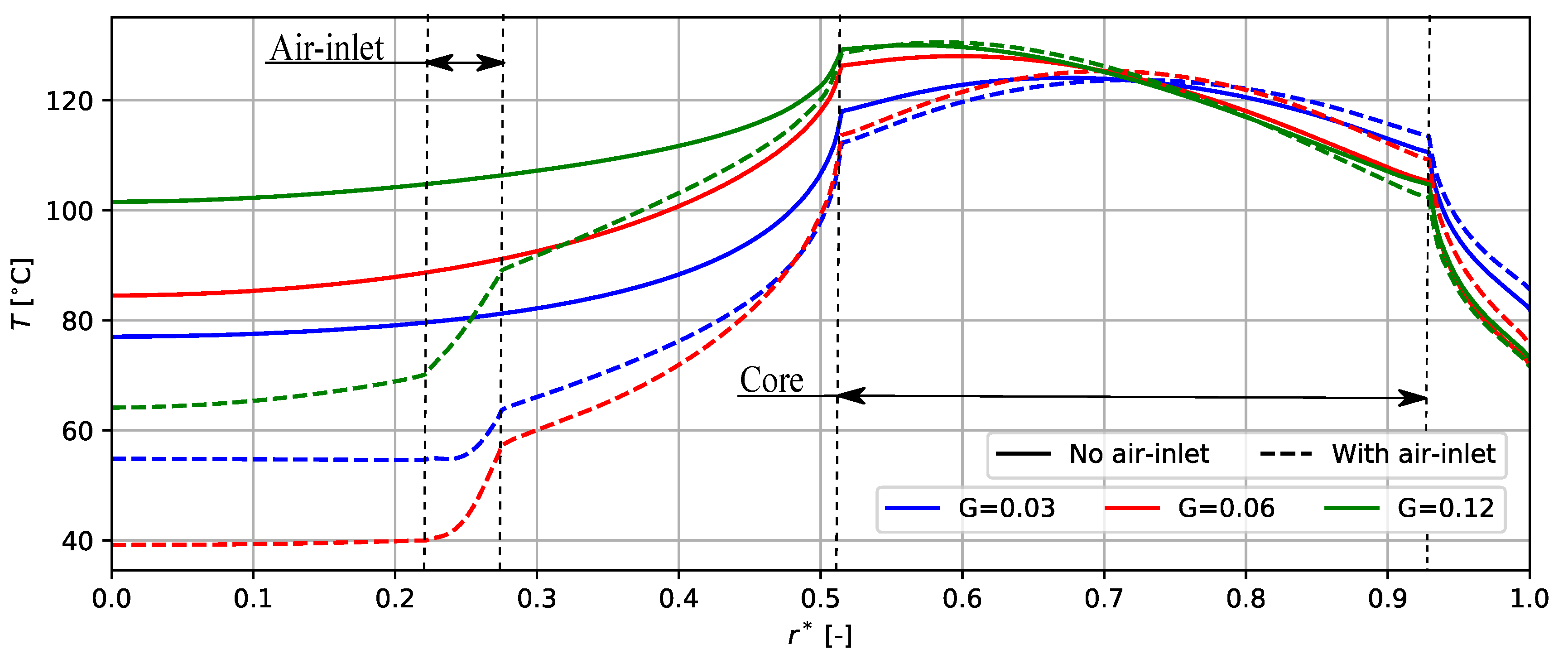
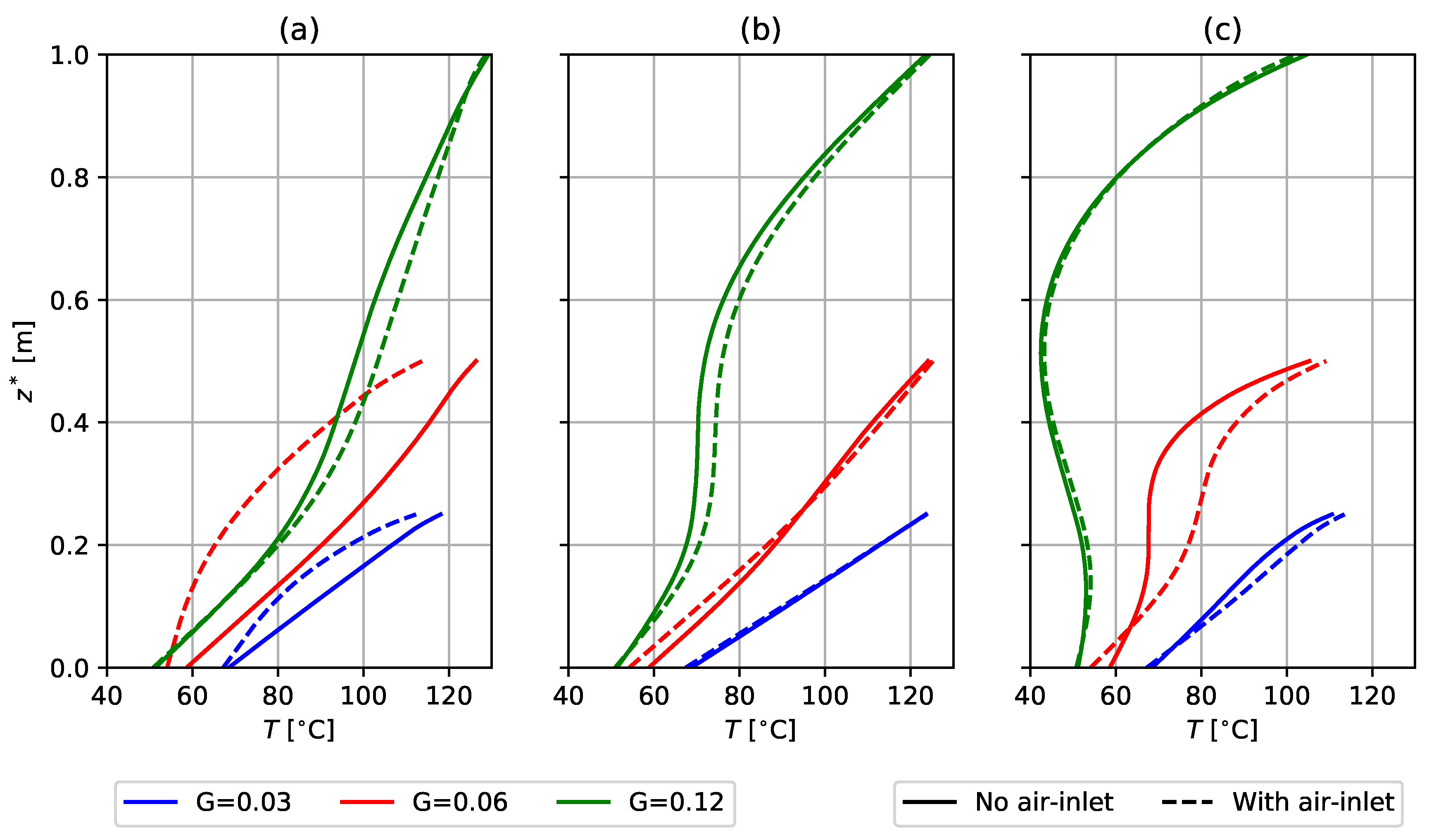
5.2. Temperature Field
6. Conclusions
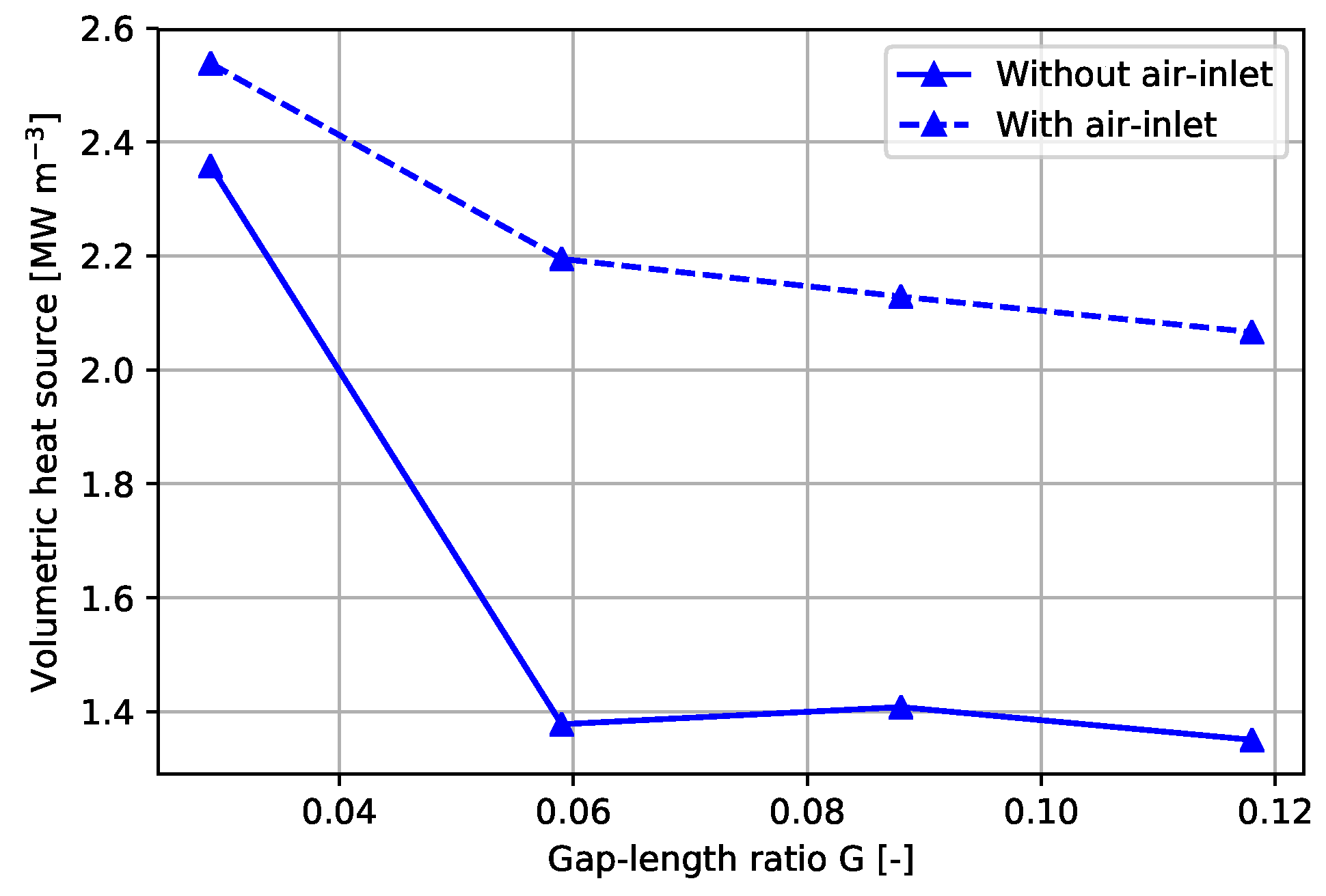
- When dealing with a partially heated stator surface, different heat transfer behavior is observed compared to the literature based on a uniformly heated stator surface. By partially heating the stator, one enables the entering fluid to dissipate its thermal energy in its path toward the axis of rotation. Decreasing the gap-length enhances this effect, as a lower surface-area-to-volume ratio is obtained, thereby effectively increasing the dissipation rate.
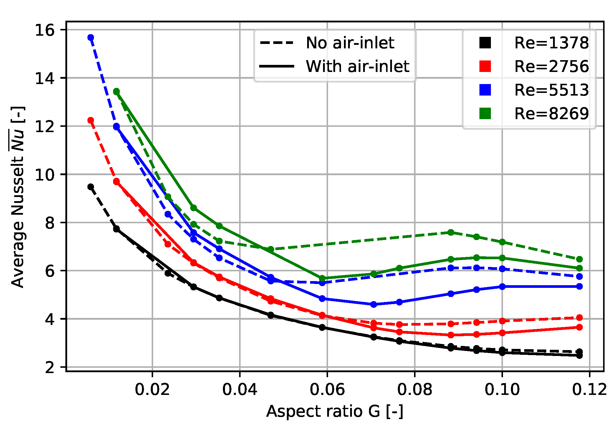
- Adding air-inlets will improve the overall cooling of the stator, but will locally worsen it inside the gap near the core surface. The main reason for this is the circulation zone at the core surface, which increases in size with an increase in gap-length or Reynolds number. It is noted that this observation for the laminar flow case does not necessarily translate to the turbulent regime.
- An air-inlet is always desired, even though the heat transfer at the core may locally become worse. The cooling through the remaining sides of the stator is expected to be substantially larger compared to having no air-inlet.
- A superposed throughflow at the air-inlet is desired over a conventional open air-inlet configuration. The reason for this is that one can then influence the flow field and therefore control the temperature of the core to some extent. The superposed flow is also able to remove the troublesome circulation zone near the core, increasing the heat transfer.
- An additional cooling circuit that could actively circulate a liquid, i.e., water, refrigerants, etc., will benefit the overall cooling of the stator. The circuit should be positioned such that it can dissipate the heat from the core both efficiently and practically, i.e., preferably located at the back of the stator disk.
- One could use highly conductive non-metal materials for the stator and rotor, dissipating the heat from critical areas even faster.
Author Contributions
Funding
Conflicts of Interest
Abbreviations
| AFPM | Axial-Flux Permanent Magnet |
| RFPM | Radial-Flux Permanent Magnet |
| FEM | Finite Element Method |
| IGA | Isogeometric Analysis |
| DOF | Degree of Freedom |
| BC | Boundary Condition |
| 3D | Three-dimensional |
| SUPG | Streamline-Upwind Petrov-Galerkin |
| DDN | Directional Do-Nothing |
| LIC | Line Integral Convolution |
| MKL | Math Kernel Library |
Appendix A. Enclosed Rotor-Stator Analytic Solution
Appendix B. Temperature Dependence

Appendix C. Material Properties

| Material | Conductivity [W/mK] |
|---|---|
| Air C | 0.030 |
| Rotor support (Aluminum) | 237.0 |
| Stator support (Resin) | 0.2 |
| Permanent magnet | 7.6 |
| Back-iron | 40.0 |
| Core (Iron M270-50A) | 25.0 |
Appendix D. Induced Heat Source

References
- Gieras, J.F.; Wang, R.J.; Kamper, M.J. Axial Flux Permanent Magnet Brushless Machines; Springer Science & Business Media: Berlin, Germany, 2008. [Google Scholar]
- Friedrich, L.A.J.; Gysen, B.L.J.; Jansen, J.W.; Lomonova, E.A. Analysis of Motional Eddy Currents in the Slitted Stator Core of an Axial-Flux Permanent-Magnet Machine. IEEE Trans. Magn. 2020, 56, 1–4. [Google Scholar] [CrossRef] [Green Version]
- Ekman, V.W. Om jordrotationens inverkan pa vindstrømmar i hafvet. Arkiv för Matematik Astronomi och Fysik 1905, 2, 1. [Google Scholar]
- Rasekh, A.; Sergeant, P.; Vierendeels, J. Development of Correlations for Windage Power Losses Modeling in an Axial Flux Permanent Magnet Synchronous Machine with Geometrical Features of the Magnets. Energies 2016, 9, 1009. [Google Scholar] [CrossRef] [Green Version]
- Howey, D.A. Thermal Design of Air-Cooled Axial Flux Permanent Magnet Machines. Ph.D. Thesis, Imperial College London, London, UK, 2010. [Google Scholar]
- Habibinia, D.; Rostami, N.; Feyzi, M.R.; Soltanipour, H.; Pyrhönen, J. New finite element based method for thermal analysis of axial flux interior rotor permanent magnet synchronous machine. IET Electr. Power Appl. 2020, 14, 464–470. [Google Scholar] [CrossRef]
- von Kármán, T. Über laminare und turbulente Reibung. Zeitschrift für Angewandte Mathematik und Mechanik 1921, 1, 233. [Google Scholar] [CrossRef] [Green Version]
- Bödewadt, U.T. Die Drehströmung über festem Grunde. Zeitschrift für Angewandte Mathematik und Mechanik 1940, 20, 241–253. [Google Scholar] [CrossRef]
- Batchelor, G.K. Note on a class of solutions of the Navier–Stokes equations representing steady rotationally symmetric flow. Q. J. Mech. Appl. Math. 1951, 4, 29–41. [Google Scholar] [CrossRef]
- Harmand, S.; Pellé, J.; Poncet, S.; Shevchuk, I.V. Review of fluid flow and convective heat transfer within rotating disk cavities with impinging jet. Int. J. Therm. Sci. 2013, 67, 1–30. [Google Scholar] [CrossRef] [Green Version]
- Stewartson, K. On the flow between two rotating coaxial disks. Math. Proc. Camb. Philos. Soc. 1953, 49, 333–341. [Google Scholar] [CrossRef]
- Childs, P.R.N. Rotating Flow; Butterworth-Heinemann, Elsevier: Paris, France, 2011. [Google Scholar]
- Zandbergen, P.J.; Dijkstra, D. Von Kármán swirling flows. Annu. Rev. Fluid Mech. 1987, 19, 465–491. [Google Scholar] [CrossRef]
- Brady, J.F.; Durlofsky, L. On rotating disk flow. J. Fluid Mech. 1987, 175, 363. [Google Scholar] [CrossRef]
- Poncet, S.; Chauve, M.P.; Schiestel, R. Batchelor versus Stewartson flow structures in a rotor-stator cavity with throughflow. Phys. Fluids 2005, 17. [Google Scholar] [CrossRef]
- Barabas, B.; Clauss, S.; Schuster, S.; Benra, F.K.; Dohmen, H.J.; Brillert, D. Experimental and numerical determination of pressure and velocity distribution inside a rotor-stator cavity at very high circumferential Reynolds numbers. In Proceedings of the European Conference on Turbomachinery Fluid Dynamics and Thermodynamics, Madrid, Spain, 23–27 March 2015. [Google Scholar]
- Debuchy, R.; Gatta, S.; D’Haudt, E.; Bois, G.; Martelli, F. Influence of external geometrical modifications on the flow behaviour of a rotor-stator system: Numerical and experimental investigation. Proc. Inst. Mech. Eng. A J. Power Energy 2007, 221, 857–863. [Google Scholar] [CrossRef]
- Itoh, M.; Yamada, Y.; Imao, S.; Gonda, M. Experiments on turbulent flow due to an enclosed rotating disk. Exp. Therm. Fluid Sci. 1992, 5, 359–368. [Google Scholar] [CrossRef]
- Jacques, R.; Quéré, P.L.; Daube, O. Axisymmetric numerical simulations of turbulent flow stator enclosures. Int. J. Heat Fluid Flow 2002, 23, 381–397. [Google Scholar] [CrossRef]
- Craft, T.; Iacovides, H.; Launder, B.; Zacharos, A. Some swirling-flow challenges for turbulent CFD. Flow Turbul. Combust. 2008, 80, 419–434. [Google Scholar] [CrossRef]
- Hemeida, A.; Lehikoinen, A.; Rasilo, P.; Vansompel, H.; Belahcen, A.; Arkkio, A.; Sergeant, P. A Simple and Efficient Quasi-3D Magnetic Equivalent Circuit for Surface Axial Flux Permanent Magnet Synchronous Machines. IEEE Trans. Ind. Electron. 2019, 66, 8318–8333. [Google Scholar] [CrossRef]
- Hill, R.W.; Ball, K.S. Direct numerical simulations of turbulent forced convection between counter-rotating disks. Int. J. Heat Fluid Flow 1999, 20, 208–221. [Google Scholar] [CrossRef]
- Pellé, J.; Harmand, S. Heat transfer measurements in an opened rotor-stator system air-gap. Exp. Therm. Fluid Sci. 2007, 31, 165–180. [Google Scholar] [CrossRef]
- Yuan, Z.X.; Saniei, N.; Yan, X.T. Turbulent heat transfer on the stationary disk in a rotor–stator system. Int. J. Heat Mass Transf. 2003, 46, 2207–2218. [Google Scholar] [CrossRef] [Green Version]
- Howey, D.A.; Holmes, A.S.; Pullen, K.R. Radially resolved measurement of stator heat transfer in a rotor–stator disc system. Int. J. Heat Mass Transf. 2010, 53, 491–501. [Google Scholar] [CrossRef] [Green Version]
- Hughes, T.J.R.; Cottrell, J.A.; Bazilevs, Y. Isogeometric analysis: CAD, finite elements, NURBS, exact geometry and mesh refinement. Comput. Methods Appl. Mech. Eng. 2005, 194, 4135–4195. [Google Scholar] [CrossRef] [Green Version]
- Bazilevs, Y.; Calo, V.M.; Hughes, T.J.R.; Zhang, Y. Isogeometric fluid–structure interaction: Theory, algorithms, and computations. Comput. Mech. 2008, 43, 3–37. [Google Scholar] [CrossRef]
- Evans, J.A.; Hughes, T.J.R. Isogeometric divergence-conforming B-splines for the steady Navier–Stokes equations. Math. Models Methods Appl. Sci. 2013, 23, 1421–1478. [Google Scholar] [CrossRef]
- Bazilevs, Y.; Hughes, T.J.R. Weak imposition of Dirichlet boundary conditions in fluid mechanics. Comput. Fluids 2007, 36, 12–26. [Google Scholar] [CrossRef]
- Carraturo, M.; Giannelli, C.; Reali, A.; Vázquez, R. Suitably graded THB-spline refinement and coarsening: Towards an adaptive isogeometric analysis of additive manufacturing processes. Comput. Methods Appl. Mech. Eng. 2019, 348, 660–679. [Google Scholar] [CrossRef] [Green Version]
- Liu, N.; Beata, P.A.; Jeffers, A.E. A mixed isogeometric analysis and control volume approach for heat transfer analysis of nonuniformly heated plates. Numer. Heat Transf. B Fundam. 2019, 75, 347–362. [Google Scholar] [CrossRef]
- Bazilevs, Y.; Veiga, L.; Cottrell, J.A.; Hughes, T.J.R.; Sangalli, G. Isogeometric Analysis: Approximation, stability and error estimates for h-refined meshes. Math. Models Methods Appl. Sci. 2011, 16, 1031–1090. [Google Scholar] [CrossRef]
- Buffa, A.; de Falco, C.; Sangalli, G. Isogeometric analysis: Stable elements for the 2D Stokes equation. Int. J. Numer. Methods Fluids 2011, 65, 1407–1422. [Google Scholar] [CrossRef]
- Evans, J.A.; Hughes, T.J.R. Isogeometric Divergence-Conforming B-Splines for the Darcy–Stokes–Brinkman Equations. Math. Models Methods Appl. Sci. 2012, 23, 671–741. [Google Scholar] [CrossRef]
- Cottrell, J.A.; Hughes, T.J.R.; Reali, A. Studies of refinement and continuity in isogeometric structural analysis. Comput. Methods Appl. Mech. Eng. 2007, 196, 4160–4183. [Google Scholar] [CrossRef]
- Dörfel, M.R.; Jüttler, B.; Simeon, B. Adaptive isogeometric analysis by local h-refinement with T-splines. Comput. Methods Appl. Mech. Eng. 2010, 199, 264–275. [Google Scholar] [CrossRef] [Green Version]
- Bazilevs, Y.; Calo, V.M.; Cottrell, J.A.; Evans, J.A.; Hughes, T.J.R.; Lipton, S.; Scott, M.A.; Sederberg, T.W. Isogeometric analysis using T-splines. Comput. Methods Appl. Mech. Eng. 2010, 199, 229–263. [Google Scholar] [CrossRef] [Green Version]
- Scott, M.A.; Li, X.; Sederberg, T.W.; Hughes, T.J.R. Local refinement of analysis-suitable T-splines. Comput. Methods Appl. Mech. Eng. 2012, 213-216, 206–222. [Google Scholar] [CrossRef]
- Van Zwieten, G.; van Zwieten, J.; Verhoosel, C.V.; Fonn, E.; van Opstal, T.; Hoitinga, W. Nutils. Available online: https://zenodo.org/record/3949893#.YEgplNwRVPY (accessed on 10 March 2021).
- Cottrell, J.A.; Hughes, T.J.R.; Bazilevs, Y. Isogeometric Analysis: Toward Integration of CAD and FEA; John Wiley & Sons: Hoboken, NJ, USA, 2009. [Google Scholar] [CrossRef]
- Kuru, G.; Verhoosel, C.V.; van der Zee, K.G.; Van Brummelen, E.H. Goal-adaptive Isogeometric Analysis with hierarchical splines. Comput. Methods Appl. Mech. Eng. 2014, 270, 270–292. [Google Scholar] [CrossRef]
- Kumar, M.; Kvamsdal, T.; Johannessen, K.A. Simple a posteriori error estimators in adaptive isogeometric analysis. Comput. Math. Appl. 2015, 70, 1555–1582. [Google Scholar] [CrossRef]
- van der Zee, K.G.; Verhoosel, C.V. Isogeometric analysis-based goal-oriented error estimation for free-boundary problems. Finite Elem. Anal. Des. 2011, 47, 600–609. [Google Scholar] [CrossRef]
- Saad, Y. Iterative Methods for Sparse Linear System. Stud. Comput. Math. 2001, 8, 423–440. [Google Scholar] [CrossRef]
- Giannelli, C.; Jüttler, B.; Speleers, H. THB-splines: The truncated basis for hierarchical splines. Comput. Aided Geom. Des. 2012, 29, 485–498. [Google Scholar] [CrossRef] [Green Version]
- Deng, J.; Chen, F.; Li, X.; Hu, C.; Tong, W.; Yang, Z.; Feng, Y. Polynomial splines over hierarchical T-meshes. Graph. Models 2008, 70, 76–86. [Google Scholar] [CrossRef]
- Wang, P.; Xu, J.; Deng, J.; Chen, F. Adaptive isogeometric analysis using rational PHT-splines. Comput. Aided Des. 2011, 43, 1438–1448. [Google Scholar] [CrossRef]
- Sederberg, T.W.; Zheng, J.; Bakenov, A.; Nasri, A. T-Splines and T-NURCCs. ACM Trans. Graph. 2003, 22, 477–484. [Google Scholar] [CrossRef]
- Scott, M.A.; Borden, M.J.; Verhoosel, C.V.; Sederberg, T.W.; Hughes, T.J.R. Isogeometric finite element data structures based on Bézier extraction of T-splines. Int. J. Numer. Methods Eng. 2011, 88, 126–156. [Google Scholar] [CrossRef]
- Dokken, T.; Lyche, T.; Pettersen, K.F. Polynomial splines over locally refined box-partitions. Comput. Aided Geom. Des. 2013, 30, 331–356. [Google Scholar] [CrossRef]
- Johannessen, K.A.; Kvamsdal, T.; Dokken, T. Isogeometric analysis using LR B-splines. Comput. Methods Appl. Mech. Eng. 2014, 269, 471–514. [Google Scholar] [CrossRef] [Green Version]
- Hansbo, P.; Juntunen, M. Weakly imposed Dirichlet boundary conditions for the Brinkman model of porous media flow. Appl. Numer. Math. 2009, 59, 1274–1289. [Google Scholar] [CrossRef]
- Nitsche, J. Über ein Variationsprinzip zur Lösung von Dirichlet-Problemen bei Verwendung von Teilräumen, die keinen Randbedingungen unterworfen sind. Abhandlungen aus dem Mathematischen Seminar der Universität Hamburg 1971, 36, 9–15. [Google Scholar] [CrossRef]
- Benk, J. Immersed Boundary Methods within a PDE Toolbox on Distributed Memory Systems. Ph.D. Thesis, Technische Universität München, München, Germany, 2012. [Google Scholar]
- Hoang, T.; Verhoosel, C.V.; Qin, C.Z.; Auricchio, F.; Reali, A.; van Brummelen, E.H. Skeleton-stabilized immersogeometric analysis for incompressible viscous flow problems. Comput. Methods Appl. Mech. Eng. 2019, 344, 421–450. [Google Scholar] [CrossRef] [Green Version]
- Hansbo, P. Nitsche’s method for interface problems in computational mechanics. GAMM Mitteilungen 2005, 28, 183–206. [Google Scholar] [CrossRef] [Green Version]
- Braack, M.; Mucha, P. Directional do-nothing condition for the Navier–Stokes Equations. J. Comput. Math. 2014, 32, 507–521. [Google Scholar] [CrossRef]
- Khalili, A.; Rath, H.J. Analytical solution for a steady flow of enclosed rotating disks. Zeitschrift für Angewandte Mathematik und Physik ZAMP 1994, 45, 670–680. [Google Scholar] [CrossRef]
- Cochran, W.G. The flow due to a rotating disc. Math. Proc. Camb. Philos. Soc. 1934, 30, 365–375. [Google Scholar] [CrossRef]
- Van Eeten, K.M.P.; van der Schaaf, J.; van Heijst, G. Boundary layer development in the flow field between a rotating and a stationary disk. Phys. Fluids 2012, 24, 033601. [Google Scholar] [CrossRef]
- Shevchuk, I.V. Convective Heat and Mass Transfer in Rotating Disk Systems, 45th ed.; Springer: Berlin, Germany, 2009. [Google Scholar]
- Elkins, C.J. Heat Transfer in the Rotating Disk Boundary Layer. Ph.D. Thesis, Stanford University, Stanford, CA, USA, 1997. [Google Scholar]
- Malik, M.R.; Wilkinson, S.P.; Orszag, S.A. Instability and transition in rotating disk flow. AIAA J. 1981, 19, 1131–1138. [Google Scholar] [CrossRef] [Green Version]
- Giovanni, A. Numerical Investigations of Air Flow and Heat Transfer in Axial Flux Permanent Magnet Electrical Machines. Ph.D. Thesis, Durham University, Durham, UK, 2010. [Google Scholar]
- Intel. Intel oneAPI Math Kernel Library (MKL). 2020. Available online: https://software.intel.com/content/www/us/en/develop/tools/oneapi/components/onemkl.html (accessed on 15 December 2020).
- Paraview. Line Integral Convolution. 2018. Available online: https://www.paraview.org/Wiki/ParaView/Line_Integral_Convolution (accessed on 9 December 2020).
- Soo, S.L. Laminar flow over an enclosed rotating disk. Trans. ASME 1958, 80, 287–296. [Google Scholar]


| [rad/s] | [m/s] | Domain Size [m] | Element nr. [-] | Spline Order [-] |
|---|---|---|---|---|
| 1.0 | 1.0 | 2 |
| Time-Step [s] | [rad/s] | [m/s] | Domain Size [m] | Element nr. [-] | Spline Order [-] |
|---|---|---|---|---|---|
| 0.02 | 1.0 | 0.2 | 2 |
| [rad/s] | [m/s] | Domain Size [m] | Element nr. [-] | Spline Order [-] |
|---|---|---|---|---|
| 1.0 | 1.0 | 2 |
[rad/s] | [m/s] | Domain Size [m] | Element nr. [-] | Spline Order [-] | Prandtl Number [-] | [-] | [C] |
|---|---|---|---|---|---|---|---|
| 1.0 | 0.2 | 2 | 0.72 | 100.0 | 20.0 |
| Disk Radius [m] | [rad/s] | [m/s] | [kg/m] | (air) [J/kgK] | Domain Size [m] | Spline Degree [-] |
|---|---|---|---|---|---|---|
| 0.17 | 0.0–6.0 | 1.0 | 1008.0 | 2.0 |
| [-] | 20,256 | 21,216 | 29,280 | 53,640 |
| [-] | 82,252 | 86,484 | 119,388 | 217,914 |
Publisher’s Note: MDPI stays neutral with regard to jurisdictional claims in published maps and institutional affiliations. |
© 2021 by the authors. Licensee MDPI, Basel, Switzerland. This article is an open access article distributed under the terms and conditions of the Creative Commons Attribution (CC BY) license (http://creativecommons.org/licenses/by/4.0/).
Share and Cite
Willems, R.; Friedrich, L.A.J.; Verhoosel, C.V. Finite Element Analysis of Laminar Heat Transfer within an Axial-Flux Permanent Magnet Machine. Math. Comput. Appl. 2021, 26, 23. https://0-doi-org.brum.beds.ac.uk/10.3390/mca26010023
Willems R, Friedrich LAJ, Verhoosel CV. Finite Element Analysis of Laminar Heat Transfer within an Axial-Flux Permanent Magnet Machine. Mathematical and Computational Applications. 2021; 26(1):23. https://0-doi-org.brum.beds.ac.uk/10.3390/mca26010023
Chicago/Turabian StyleWillems, Robin, Léo A. J. Friedrich, and Clemens V. Verhoosel. 2021. "Finite Element Analysis of Laminar Heat Transfer within an Axial-Flux Permanent Magnet Machine" Mathematical and Computational Applications 26, no. 1: 23. https://0-doi-org.brum.beds.ac.uk/10.3390/mca26010023