
Application of Data Assimilation and the Relationship between ENSO and Precipitation


Department of Mathematics, Faculty of Science, King Mongkut’s University of Technology Thonburi, 126 Pracha Uthit Rd., Bang Mot, Thung Khru, Bangkok 10140, Thailand
*
Author to whom correspondence should be addressed.
Math. Comput. Appl. 2021, 26(1), 24; https://0-doi-org.brum.beds.ac.uk/10.3390/mca26010024
Submission received: 12 January 2021
/
Revised: 4 March 2021
/
Accepted: 8 March 2021
/
Published: 12 March 2021
Abstract
:Climate change in Thailand is related to the El Niño and Southern Oscillation (ENSO) phenomenon, in particular drought and heavy precipitation. The data assimilation method is used to improve the accuracy of the Ensemble Intermediate Coupled Model (EICM) that simulates the sea surface temperature (SST). The four-dimensional variational (4D-Var) and three-dimensional variational (3D-Var) schemes have been used for data assimilation purposes. The simulation was performed by the model with and without data assimilation from satellite data in 2011. The result shows that the model with data assimilation is better than the model without data assimilation. The 4D-Var scheme is the best method, with a Root Mean Square Error (RMSE) of 0.492 and a Correlation Coefficient of 0.684. The relationship between precipitation in Thailand and the ENSO area in Niño 3.4 was consistent for seven months, with a correlation coefficient of −0.882.
1. Introduction
In 2011, Thailand experienced the worst flooding in its history, suffering heavy floods for a long time. The affected areas were spread around the country, but they were especially concentrated in the northern and central regions. Moreover, Bangkok and its suburbs are areas that have endured heavy floods for the last 70 years. The floods have caused great damage to agricultural, industrial, economic, and social life, and they have had a high impact on other sectors. Thailand was flooded and 64 provinces were declared to be emergency disaster zones from the end of July to November 2011. There were 657 deaths, three missing people, 4,039,459 destroyed households, and 13,425,869 displaced people. In the case of 2329 houses, the entire property was damaged, and a further 96,833 houses were partially damaged. The damage extended to an estimated 1.792 million hectares of agricultural area, 13,961 roads, 777 drains, 982 dams, 724 bridges/semis, 2324,919 fish ponds/shrimp ponds, and 13.41 million ranches [1]. This massive flood, including many other events, was the result of the ENSO phenomenon.
The El Niño and Southern Oscillation (ENSO) phenomenon affects climate around the world, especially countries that are near the equator around the Pacific Ocean. It is a term used to describe changes in SST in the Pacific region, and variations in the southern hemisphere climate systems [2]. Strong trade winds blew to the east, so that the sea level in the Western Pacific Ocean was higher than usual. The El Niño is a phenomenon where the atmospheric pressure at sea level in the eastern Pacific Ocean is lower than usual, while the other side of the ocean pressure (Indonesia and northern Australia) is higher than usual. It connects and occurs along with the weak south-east wind until it becomes a western wind. It will blow the sea from the west Pacific Ocean to the central and eastern Pacific Ocean. The scientists often used the terms of ENSO warming (ENSO warm event or warm phase of ENSO) as same as the meaning of El Niño for describing the phenomena that the SST in the central and eastern Pacific are warmer than the normal. La Niña is an abnormally cold ocean temperature phenomenon (ENSO cold event or cold phase of ENSO). It is used to describe the phenomena where the SST in the central and eastern Pacific are cooler than the normal. The La Niña phenomenon first appeared in early 2011 [3]. The ENSO phenomenon is linked to climate anomalies in far-flung areas, such as Australia, which is subjected to year-round drought, causing wildfires and the Indian peninsula to suffer from year-round rainfall. As a result, the current weather conditions have changed [4]. Therefore, it is necessary to forecast the occurrence of ENSO phenomena in order to determine exposure to climate change. There are currently models for predicting the occurrence of various types of ENSO phenomena, such as [5,6,7,8,9]. Although the ENSO phenomena are continuously and intensely studied, there is still significant uncertainty in real-time predictions of ENSO phenomena. The accuracy of the forecast is reduced when it is forecasted during the northern spring. The phenomenon of spring predictability barrier (SPB) is known as one of the main factors limiting the ENSO’s predictive skills [10,11,12]. There are many studies that try to reduce the predictive error of the ENSO phenomenon. An effective method is using a Nonlinear Forcing Singular Vector [13,14]. For the ENSO forecast system, most of the model systems are freely integrated for a specific time interval (i.e., the prediction time period) after assigning an initial value by assimilation when they predict ENSO. However, Tao and Duan [15] and Tao et al. [16] proposed a novel method to predict ENSO. They adopted an approach of nonlinear forcing singular vector-assimilation to predict ENSO, in which it considers a model error effect and it is different from three-dimensional (3D)- and four-dimensional variational (4D-Var) assimilation for the initial error effect.
Data assimilation is a statistical technique that combines the result of the mathematical model with observational data to improve the accuracy of the simulation. The objective of this work is to compare three-dimensional (3D-Var) and four-dimensional (4D-Var) data assimilation methods for heavy rain in Thailand. The benefit and drawback of the two methods were compared to evaluate their practical application. The 3D-Var method is considered to be an economically and statistically reliable method, and it is widely accepted. The 4D-Var method is an advanced technique of data assimilation that best fits the observations distributed within a given time interval. Therefore, this work aims to improve the forecasting of the ENSO phenomenon in the Pacific Ocean while using the 3D-Var and 4D-Var method, and to establish the relationship between ENSO phenomenon and precipitation in Thailand.
2. Materials and Methods
2.1. Ensemble Intermediate Coupled Model
The atmosphere and oceans are two major components in the Earth’s system. The atmospheric models measure the number of spatial changes of atmospheric phenomena in space and time. Numerical and physical measurements of weather parameters were used to study and predict the occurrence of phenomena [17]. The ocean dynamics model causes the variation of seawater, such as temperature or motion of water. The atmosphere and the ocean are connected in a complex way. Both of the systems have a major impact on Earth’s systems, such as weather and climate. The oceans regulate weather systems by delivering humidity and heat to the atmosphere system. Furthermore, the atmosphere is related to the ocean through momentum, humidity, heat, and wind flow. ENSO originated from the relationship of the ocean with the atmosphere in tropical Pacific Ocean. A coupled model between the atmosphere and ocean model is necessary for performing an ENSO. Therefore, ENSO phenomena forecasting is required to use atmospheric data, as the atmosphere influences ocean dynamics. The couple model considers various factors that affect the performance of the ENSO phenomenon. Currently, the atmosphere–ocean coupling model can predict the ENSO phenomenon over a one-year period. Most of the observational data have irregular distances. The quality control of the initial data is processed by the assimilation data.
Keenlyside and Kleeman (2002) [18] and Zhang et al. (2003) [19] developed the intermediate couple model. The ocean element of the Intermediate Coupled Model (ICM) is dependent on an intermediate complexity model that was an enlargement of the Coupled Model and Baroclinic model. The Dynamic Ocean Model contemplates some non-linear effects in simple ocean modeling contexts and differentiation of the spatial stratification to help advance simulation progress. Dynamic Ocean modeling takes into account ocean pressure fields, horizontal currents above mixed layers, vertical velocity surfaces at the base of the mixed layer, and 10 vertical modes are included in the field calculation. The thermodynamic process of the composite layer of the surface was created from a combination of the anomalous SST model and the intermediate ocean model. The model domain spans tropical Pacific from S to N and from E to W. The Extended Reconstructed Sea Surface Temperature (ERSST) grids are , but the data of the EICM are different grids point, in which a distance of Longitude is , and Latitude is different, depending on the distance of equator. The area that is far equator line has distance and the area that is near the equator line has distance . The grid of the EICM should be adjusted by linear interpolation, so that the two grids are the same size.
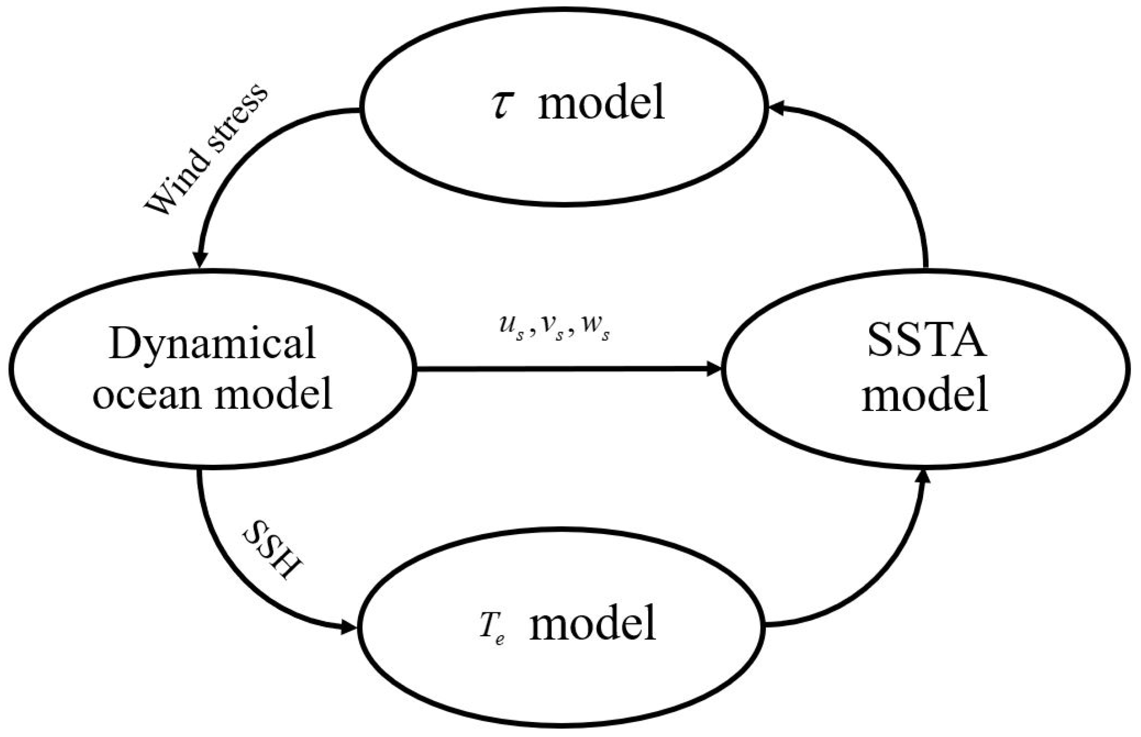
The governing equation of the fault model of SST is powered by ocean horizontal advection and vertical circulation connected with the specified and anomalous mean currents, explaining the evolution of temperature anomalies in the mixed layer, as shown in Figure 1. Another important characteristic that is added to the ocean model is the empirical determination of the temperature of the subsoil confined to the mixed layer (), which is appropriately calculated in the term of the Sea Surface Height (SSH) anomaly. Vertical mixing and buoyancy are essential conditions for clearly controlling the combined heat budget over the equatorial Pacific Ocean. It affects the SST, which is sensitively dependent on [20]. The velocity specified in the east () west () and vertical () direction is optimally calculated for the effective improving of the SSTA simulation in the ocean model, and the empirical scheme was expanded as a parameter . An inverse simulation of the given SSTA equation with balancing the various heat budget requirements of mixed layers is used to estimate the optimized field. Other ocean dynamic variables (e.g., sea level) were used in the standard statistical analysis from 1963 to 1996 for the SSTA [20] simulation. The parameterization made it possible to capture the non-local relationship between and sea level (SL) anomalies over the tropical Pacific Ocean, and this led to an explanation of improvement of the underground effect on the SST variance of the mean increase of the anomalous underground temperature anomaly. The ICM is widely used to simulate and predict El Niño phenomenon in the tropical Pacific Ocean, so the SSTA simulation has been significantly improved over the Pacific.
In addition, the ICM for the tropical Pacific Ocean was obtained from the ocean model, which was coupled with the simple statistical model of interannual wind stress anomaly (). ICM was able to demonstrate the interannual variation, which was extensively analyzed while using observational data with appropriate model parameters. Especially, the ICM can realistically explain the evolution of time and spatial structure in predicting interannual SST. Since 2003, this model has often been used to predict SST conditions in the tropical Pacific with a lead time of 12 months [9,21].
The Ensemble Intermediate Coupled Model (EICM) was developed from ICM to improve the ENSO phenomenal forecasting results [22] using a different method to generate initial ensemble members with the Markov stochastic random model. The Evensen study [23,24] was also used to provide a set of initial conditions for an ICM with 100 members. The covariance of the initial model background error between the state variables after the serial assimilation cycle was consistent with the covariance of the observation error. The observation error is shaped like the horizontal distribution of the model instability. Therefore, each ensemble member after mixing may represent one type of true condition and the band state variable. The EICM can portray interannual variability very well with a dominant four-year oscillation period [19,20]. Furthermore, this based structure was also taken as a guideline for Ocean General Circulation Model (OGCM) based Hybrid Coupled Model (HCM) simulations and ENSO predictions [25,26].
The advantage of EICM over an OGCMs is that their simplicity allows them to be used for mechanism analysis. This is well recognized, and other efforts have been made to improve the simulation of zonal currents and SST in EICMs [27,28]. The improvements in these models have only been achieved by the addition of high order baroclinic modes. These models are less realistic than the model with data assimilation. The equation for sea surface temperature anomaly (SSTA) that is implemented in the SST (sea surface temperature) component is calculated by Equation (1),
where and are anomalous sea surface temperature and water temperature below mixed layer, and represents the subsurface entrainment temperature. The specified seasonally varying mean SST is represented by and . is the Heaviside step function; is the surface heat flux term that is parameterized as being negatively proportional to the local SST anomalies with the thermal damping coefficient. and are the prescribed seasonally varying mean zonal and meridional currents in the mixed layer, and is the prescribed seasonally varying mean entrainment velocity at the base of the mixed layer, which is all obtained from the dynamical ocean model. , , and are the corresponding anomaly fields. H is the depth of the mixed layer. is the depth of the second layer [29], is the coefficient for horizontal diffusivity, is the coefficient for vertical diffusivity, and is the horizontal divergence operator.
2.2. Three Dimensional Variational Models
There are many methods of data assimilation to simulate the SST in the Pacific Ocean. It is generally very difficult to find the correct background variance. However, the accurate estimation of covariance for data assimilation is still a difficult statistic. Several statistical methods are used to obtain the estimation of covariance, which consists of (1) reducing variance of error analysis to a minimum (by weighing the right through the least squares method) and (2) variation methods (finding an analysis that reduces the cost function, which is the distance measurement of both background analysis and observation). Variance methods have become the most commonly used data assimilation technique in modern numerical weather predictions. This is because of the advantage of allowing one to eliminate the initial startup procedures being used in the 3D-Var analysis and in accordance with finding the best analysis field. It is a function cost reduction. For example, the cost function is defined as the sum of the distance between background field and by the inverse weight of the common background variances and the distance from the observed y, being weighted by the inverse of the covariance error observation. In mathematics, the cost function is
where is cost function, is background field, is observation field, is the background error covariance, is the observational error covariance, and is the linear observation operator matrix. In 3D-Var, there is no selection for a limited number of observations within the boundary of the grid point. All of the observations are used at the same time, which leads to smoother analysis. The forecast variability or background error is determined using fewer assumptions in 3D-Var, especially a method called National Meteorological Center (NMC) [30].
2.3. Four-Dimensional Variational Models
Four-Dimensional Variational models are referred to as 4D-Var. The 4D-Var method evaluates the parameter of the model between observations and model prediction by optimization (see Equation (3)). The optimization procedure is the adjustment process that enables the prediction result to be as close as possible to the observation value. The method of 4D-Var is similar to 3D-Var, in which the cost function is still the same, but it includes time considerations. The “4D” nature of 4D-Var indicates the fact that the observation set only spans 3D-space, but it also includes the time domain. The characteristic 4D-Var is that time enters as a supplementary component. 4D-Var searches for an optimal set of model parameters (such as the model’s initial optimum state), thereby reducing discrepancies between the model forecast and the time at which the observational data were distributed through the assimilation window [31]. The technique of this modeling is to find the model’s initial conditions, , in order to partially reduce the scalar quantity, J. The cost function is the function that depends on state vector . It is defined as a measure of the fit that simultaneously occurs during predicting the present true atmospheric state. One of these versions is self-observation and the other is based on model predictions. The observational data are composed of vector . The measurements of observation do not cover all of the atmospheres, so the initial data do not use observations alone. Additionally, different observations are not necessarily required to provide independent information, and priority information is needed for simulation. This is the second version of the atmospheric state used in the cost function, and it is derived from previous model predictions. This state is called the background , which is valid at the time , serving as “fillers” for data gaps. The formula of function J is defined as (i) the background, and the model state (ii) predicted observations and model state [32].
where is the background or first guess at , and are the vector of observations made at time and its corresponding observation error covariance, is the background error covariance, is the model state at the observation time that was obtained by integrating the non-linear model , and H is the (nonlinear) observation operator at time that maps model variables to observation variables. The control variable is the model state vector at the beginning of the window . This is a strong constraint minimization, in which the analysis valid at is given by the model forecast .
2.4. Strategy
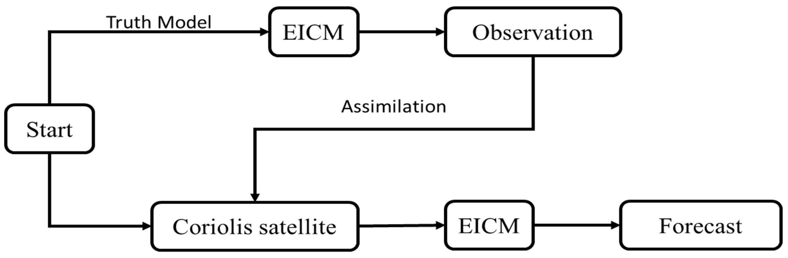
The EICM uses input data, namely SST data from ERSST with a resolution of two degrees. The data sources used to improve the accuracy of the model using assimilation are the data collected from the Coriolis satellite. The calculations of the assimilation method are based on satellite data until the end of the forecast, and then the model will get the new prediction data of SSTA. Figure 2 shows the working process of the assimilation method.
Visual comparisons are, of course, not sufficient for assessing the accuracy of the data assimilation and the model, so further tests are performed with statistical parameters, such as the Correlation Coefficient (R) and Root Mean Square Error (RMSE). The results from model and satellite data in 2011 were used for statistical accuracy testing according to the following equation:
Root Mean Square Error
Correlation Coefficient
From the above equation, is the SSTA data from EICM data, is the SSTA data obtained from the buoys in each grid. is the mean SSTA data from EICM data. is the mean SSTA data that are obtained from the buoys in each grid.
3. Results and Conclusions
3.1. Results
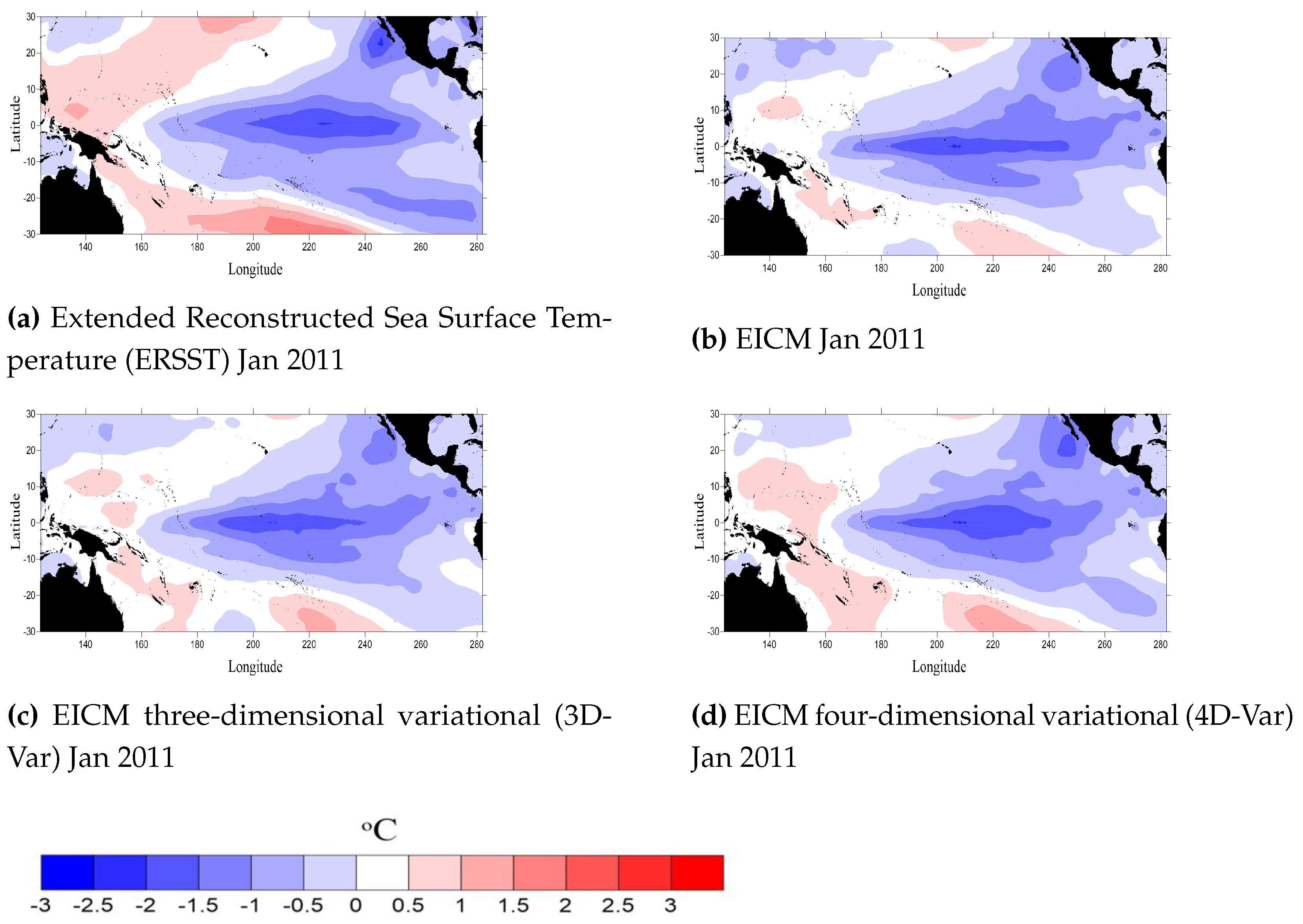
The model’s results were compared with the observed data in 2011. The prediction of the SST values of the model with and without data assimilation are called EICMDA and EICM, respectively. The results of the two simulations were compared with observable data in order to determine whether the data assimilation algorithm was working properly. A preview of the SSTA results from each simulation was compared with the observations made in these months to assess the accuracy of the preliminary model. Figure 3, Figure 4, Figure 5 and Figure 6 shows SSTA forecasts for Niño [33,34,35] and the Pacific Ocean (31 S to 31 N, 124 W to 282 W) from EICM and EICMDA in January, March, June, and September 2011 using data starting from December 2010, February 2011, May 2011, and August 2011, respectively. During the severe La Niña incident in January, all three simulations gave SSTAs that were less than the 30-year average. The forecast results of EICMDA with 4D-Var (Figure 3d) gave SSTA values of less than EICM (Figure 3b) and EICMDA with 3D-Var (Figure 3c), which are more closely matched to the measurements from ERSST (Figure 3a) at the Niño region. In the western Pacific region, EICMDA with 4D-Var gives higher SSTA than the 3D-Var method and EICM, respectively.
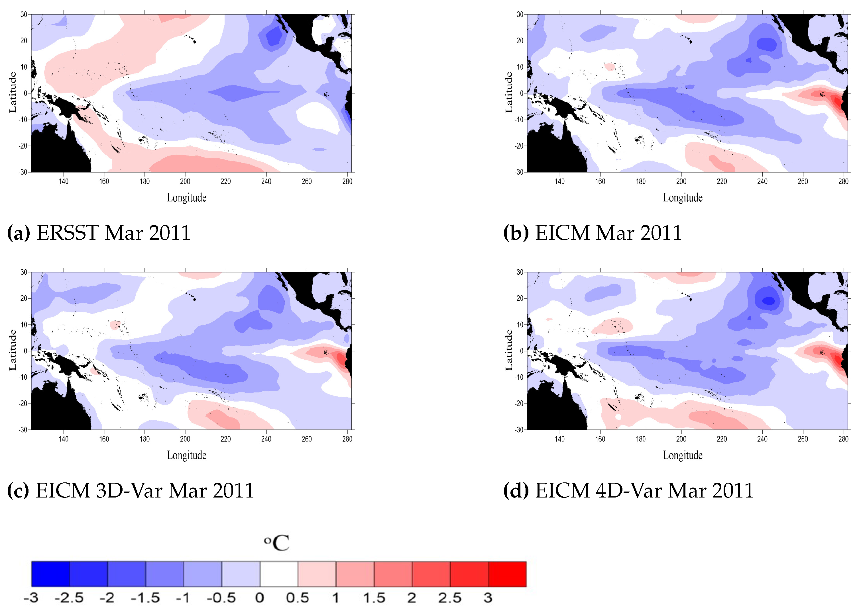
In March, when the weak La Niña phenomenon occurred, all three simulations showed an increase in SSTA values over the 30-year average in the Niño region, which was different from the measurement data (Figure 4a) that SSTA will increase, but still less than the 30-year average. In the west of the Pacific, the 4D-Var method (Figure 4d) also had an increased SSTA than 3D-Var method (Figure 4c) and EICM (Figure 4b).
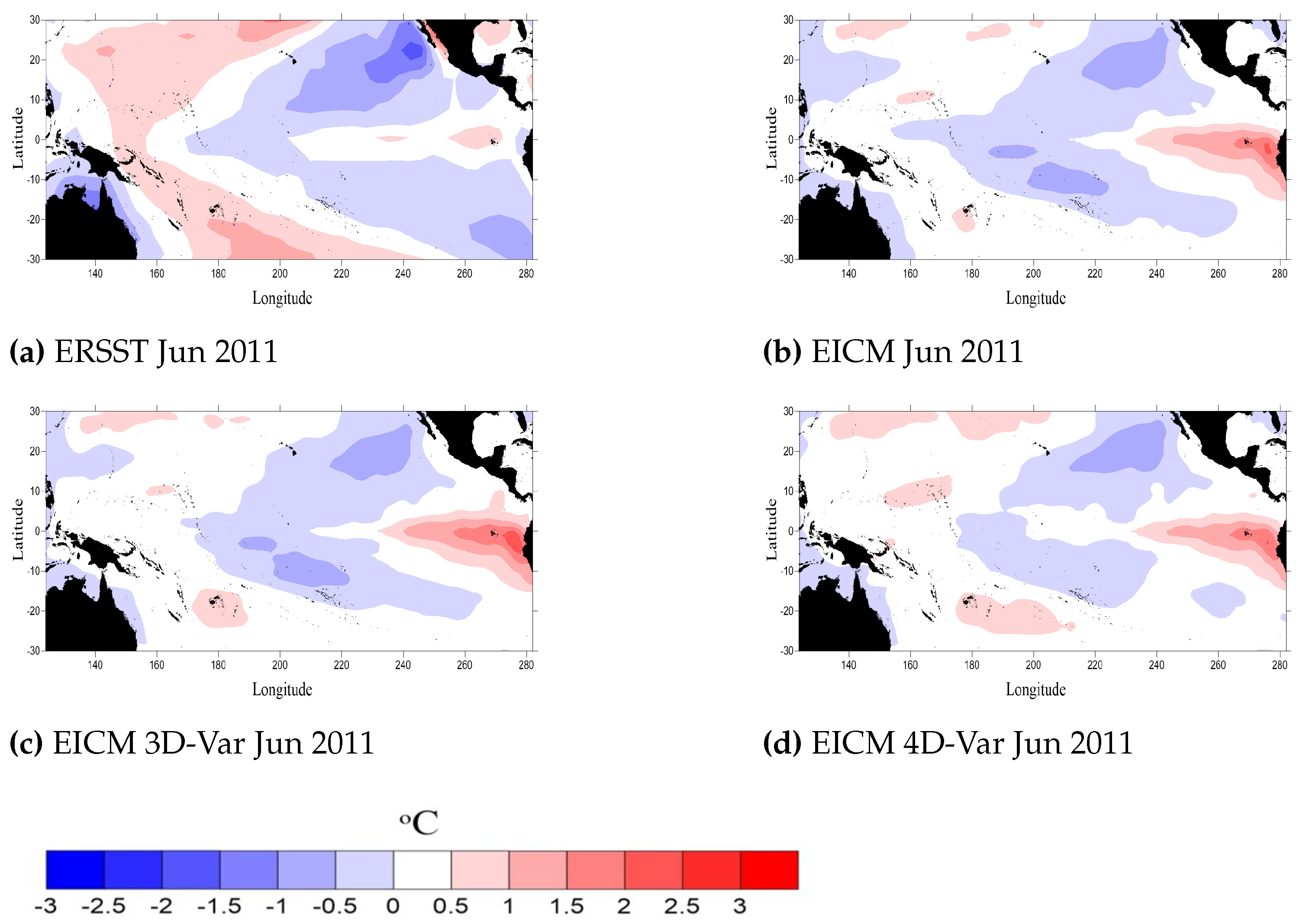
During the period of neutral state (June), it was found that the three simulations gave no significant difference in their forecasting values. However, it was found that the SSTA of the 4D-Var method was closer to the measurement data than 3D-Var and EICM at Niño region, respectively (Figure 5a–d).
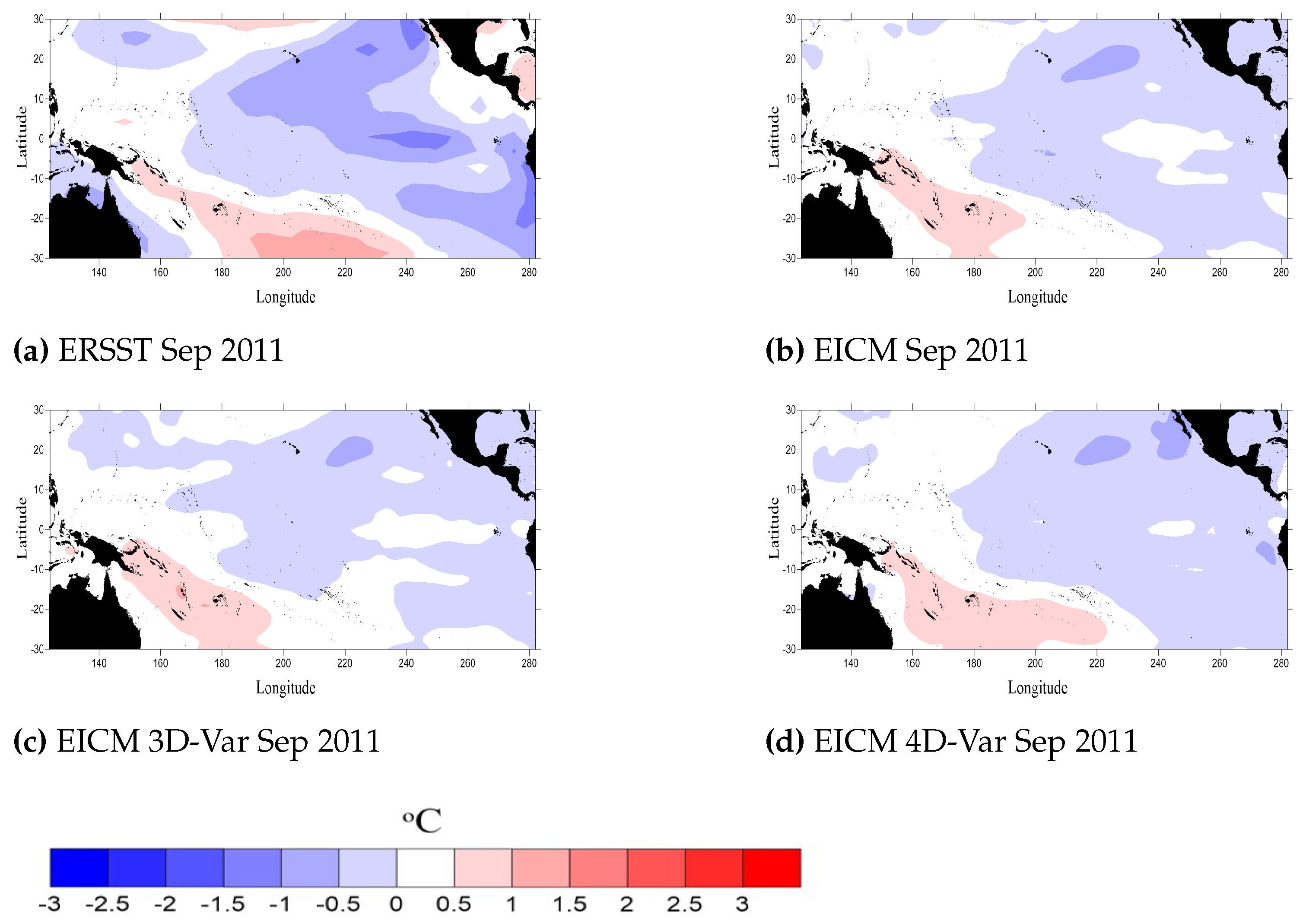
During the weak La Niña phenomenon (September), the result of 4D-Var method (Figure 6d) showed less SSTA than 3D-Var method and EICM model (Figure 6b,c, respectively). In the south of the Pacific and NINO area, the forecast results of the 4D-Var method have SSTAs that are close to the ERSST measurement data. When forecasting for all 12 months during the La Niña phenomenon, it was found that the 4D-Var method still gave less SSTA value than 3D-Var and EICM. The forecast is not very different, as shown in Figure 6.
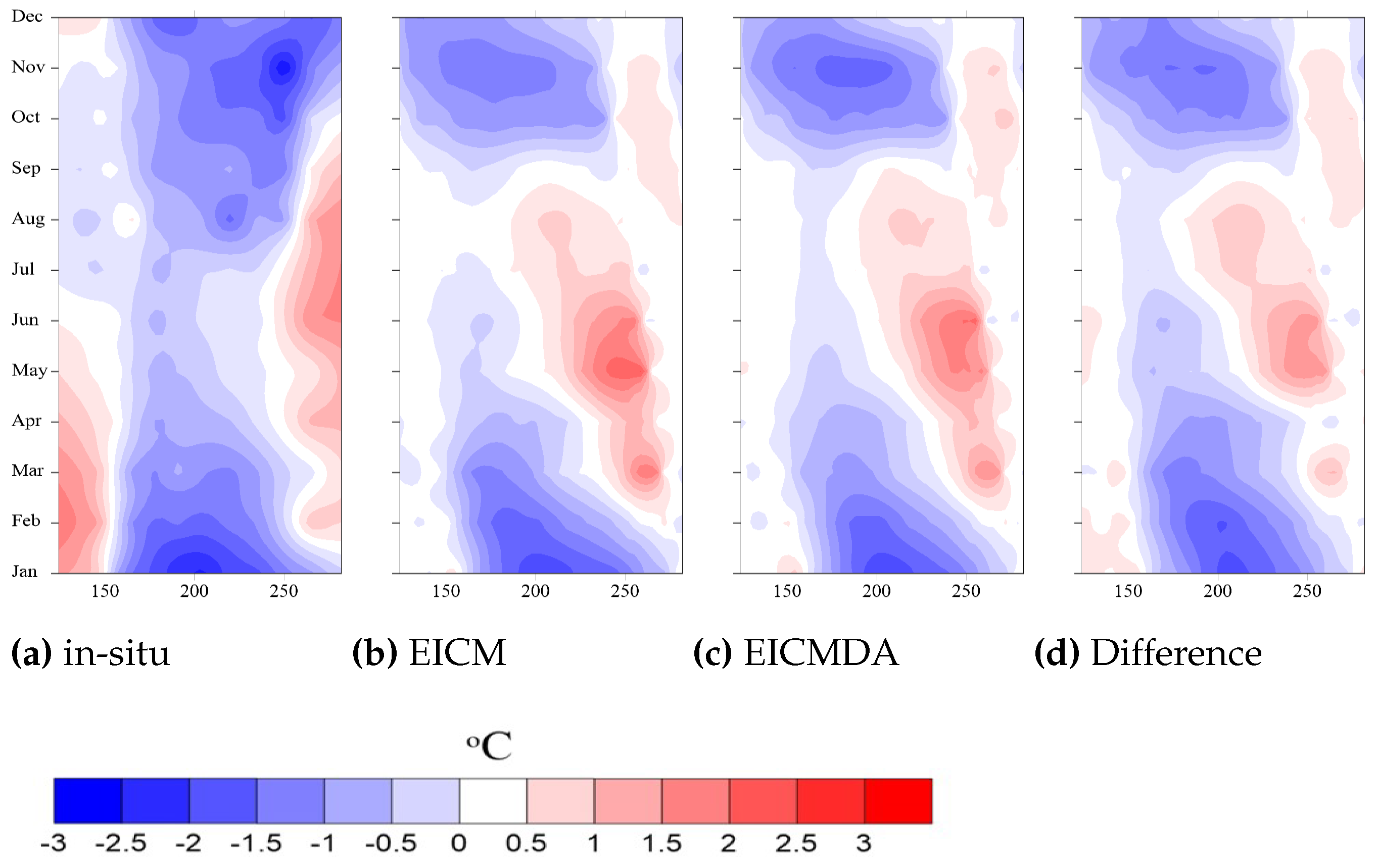
Figure 7 shows a comparison of SSTA values at the equator in 2011. The blue area shows the SST, which is 30 years below the average SST. The white area shows the SST that is equal to the average SST over the last 30 years. The red area shows the SST that is 30 years higher than the average SST. In the forecast, it was found that the SSTA values that were predicted by the three simulations are higher than the data from floating buoys. According to the SSTA forecast during the La Niña occurrence from January to May, the EICMDA provide an SSTA closer to the observed data than the EICM simulation. In a normal period from June to September, the EICMDA has less SSTA than the EICM and it provides data that are close to the observation. The EICMDA system yielded warmer SST anomalies than the EICM in the eastern tropical Pacific.
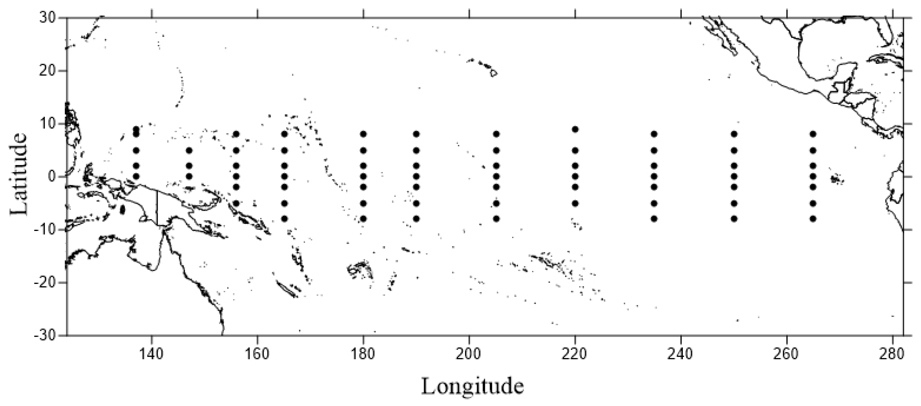
A comparison of the accuracy of the EICMDA and EICM simulations was obtained from the NOAA/PMEL TAO buoy network [36,37], where Figure 8 shows the buoy location in the central Pacific Ocean that predicts ENSO-related climate variations.
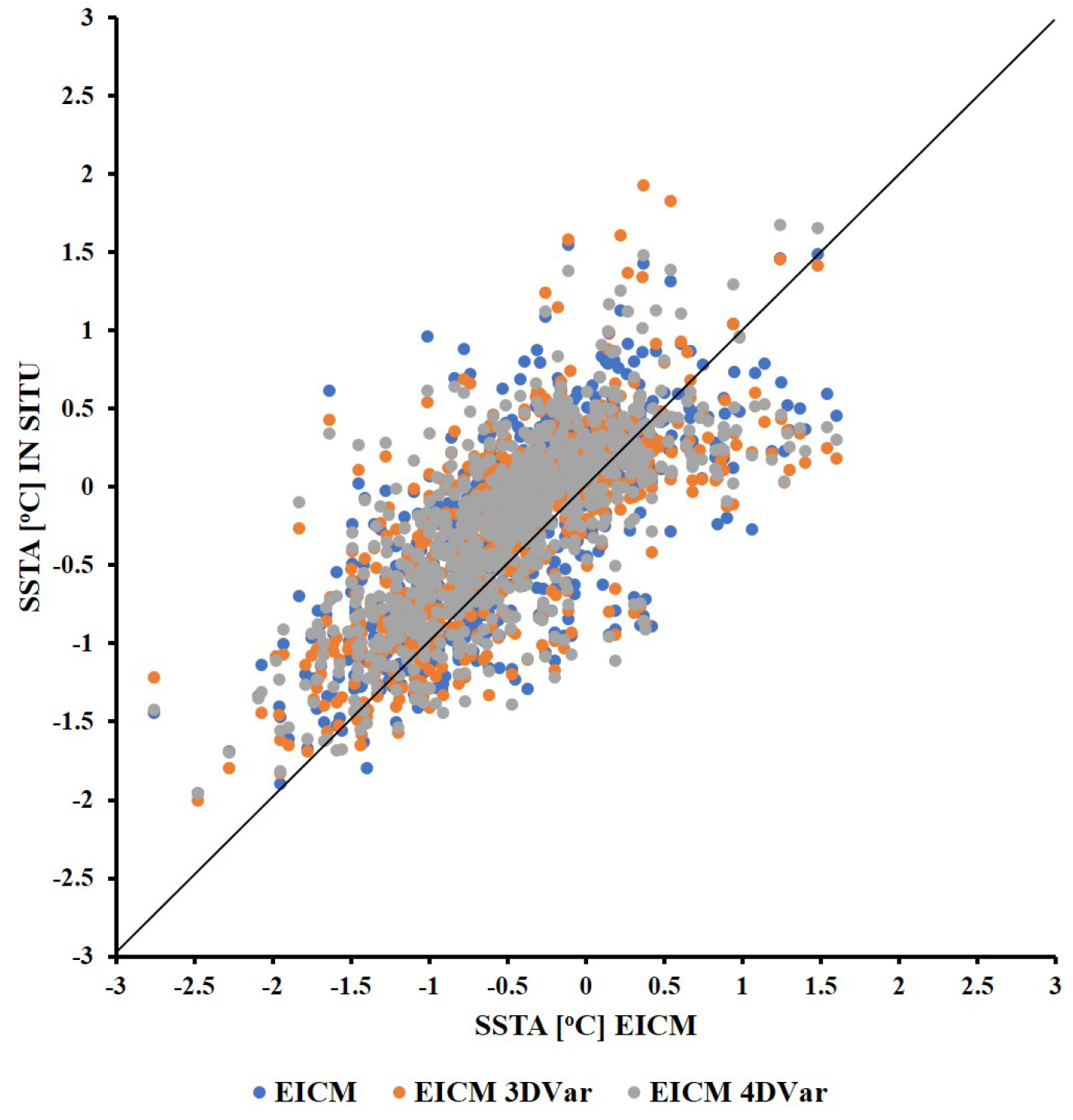
The understanding of the relationship between variables is a very important aspect of statistical analysis. Scatter plots are used to observe correlations between the result of the model. In this work, the SSTA was modeled in three simulations: the EICM and EICMDA simulations with 3D-Var and 4D-Var methods. A scatter plot uses points to explain the SSTA values from each simulation, as shown in Figure 9. The location of each point on the vertical and horizontal axis indicates SSTA values for an individual data point. Figure 9 compared the performance of the three assimilation algorithms with the in-situ data, and found that the values of each SSTA were not very different. The EICM 4D-Var has less SSTA variance than the other methods, which can be seen in less SSTA distribution than the other methods. EICM without Data Assimilation had greater SSTA variability and, for the three simulations, the majority of SSTAs were less than the in-situ. The distribution of points in the scatter diagram represents the greater relationship between the data.
The performance of the model was achieved by comparing the SSTA data of the three simulations with the SSTA data from the buoy, with each data point being compared, as shown in Figure 8. The main statistical parameters were calculated separately for each month. It was found that, during the La Niña phenomenon from January to June, the EICMDA was more accurate than EICM without Data Assimilation. In the normal period, it was found that EICMDA and EICM can simulate very different SSTA values, whereby EICMDA with 4D-Var has a lower error than the EICMDA with 3D-Var and EICM simulation. The average RMSE of EICMDA with 4D-Var is 0.492, which is the smallest error when compared to other methods. When looking at the correlation between the model and the source data, it was found that the average correlation coefficient was 0.684, which means that the data from the model correlated with source data in the same way. The correlation coefficient from the three simulations gave little difference, as shown in Table 1.
From Table 1, it was found that the RMSE values of all three simulations had little difference, because comparison with statistical data takes the data one month in advance. When comparing the three-month, six-month, and nine-month prediction results, it was found that the RMSE value varied more. The three-month forecast had a difference of 0.02 for RMSE. The six-month and nine-month forecast had a difference of RMSE is 0.07, as shown in Table 2.
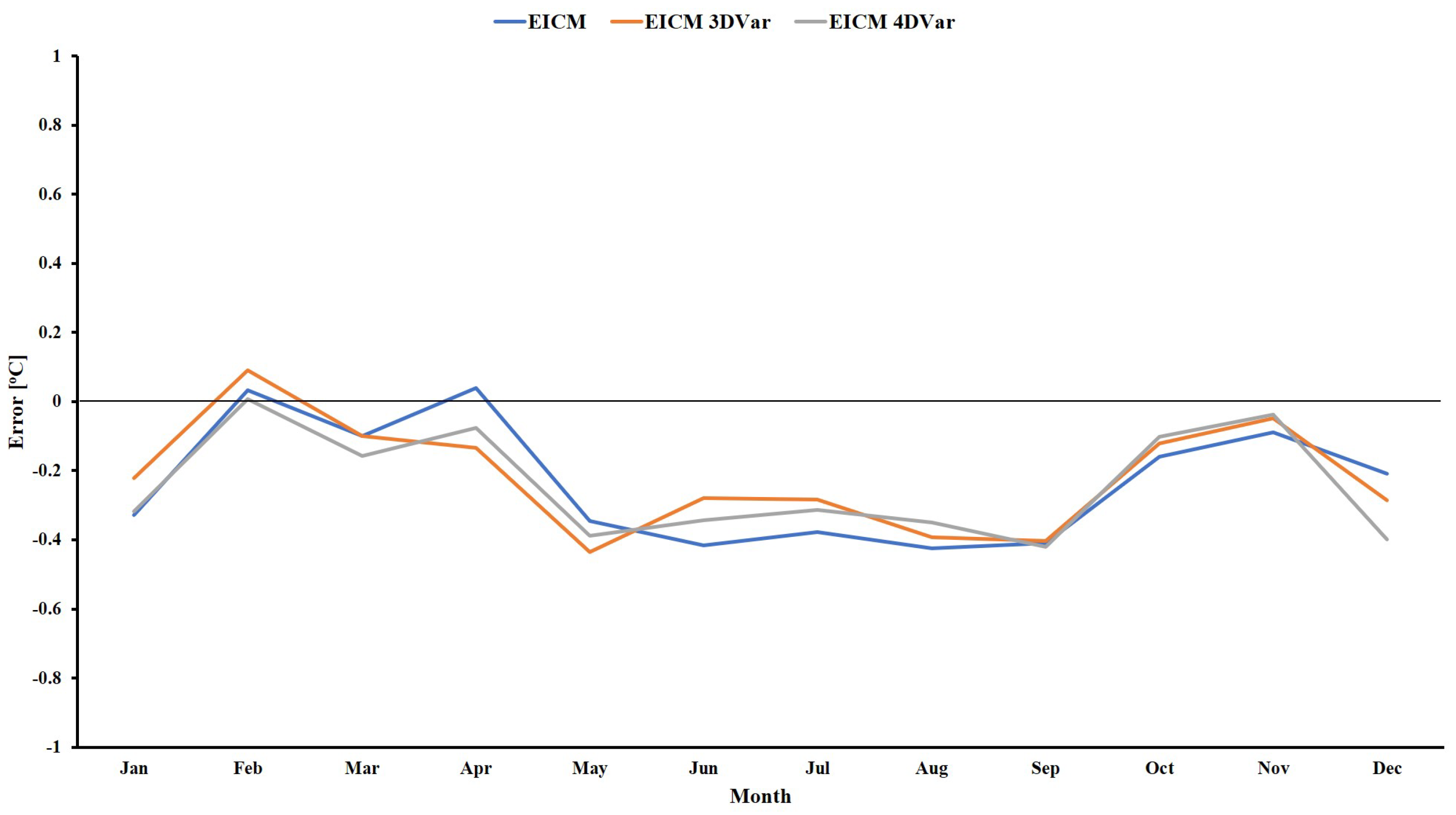
An error describes the difference between a simulation value and observation value. A comparison of the monthly error showed that, when the ENSO phenomenon occurred in the period of January to April and October to December, as shown in Figure 12, all three simulations were able to calculate the anomalies of temperature close to the source data, with the tolerance approaching 0. In the range not exceeding the ENSO phenomenon, the EICMDA gives a tolerance of 0.3, which is less than the EICM, which gives a tolerance of 0.4, as shown in Figure 10. During April to May, the tolerances of the EICM without data assimilation were significantly larger than the EICMDA. It can be seen that the model with data assimilation gives a lower tolerance.
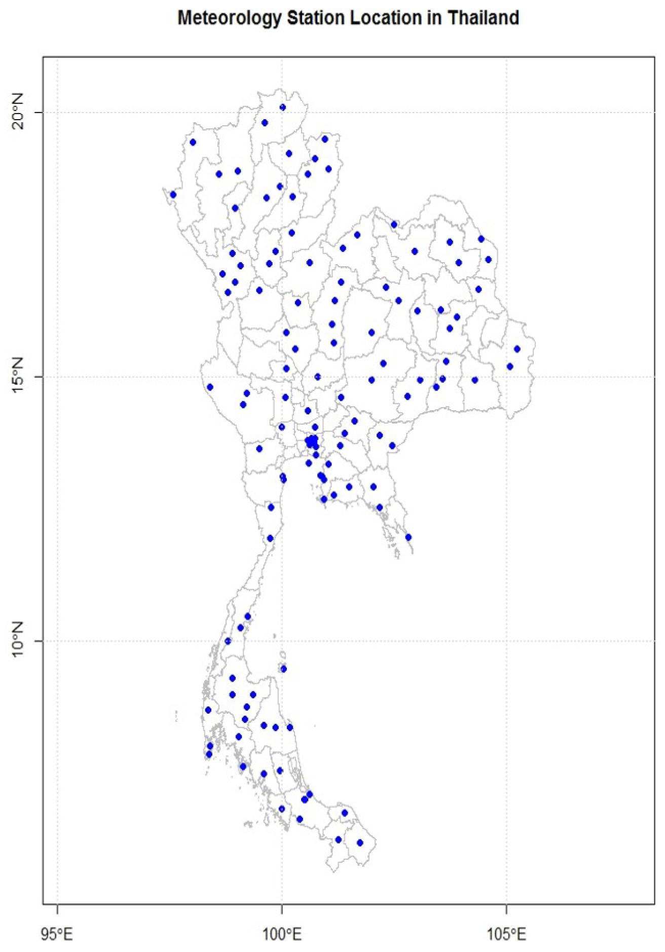
The relationships between the ENSO phenomenon and precipitation in Thailand by using data from 124 stations of the Thai Meteorological Department, which is the monthly average precipitation data in 2011 and 2012, are shown in Figure 11. This is used to study the climate impacts on Thailand.
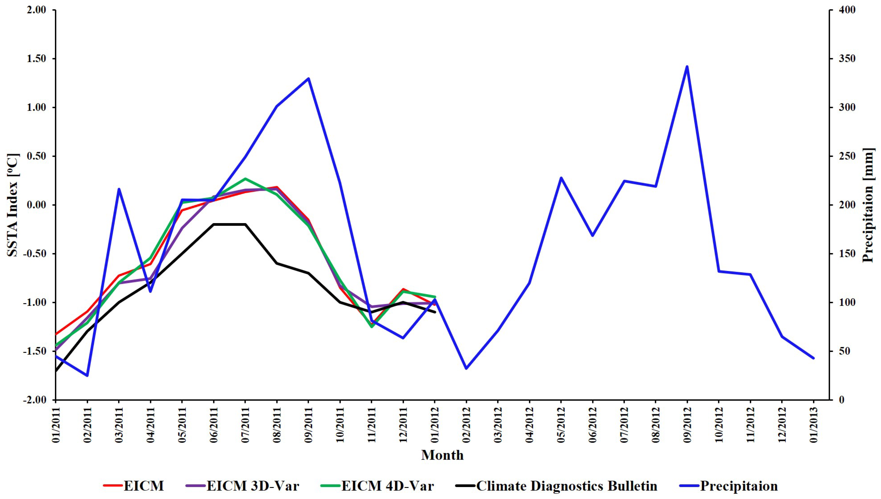
Table 3 shows the correlation coefficient between the precipitation from Meteorological Department in Thailand and the SSTA data from the EICM, EICMDA simulation, and measurements data (from Climate Diagnostics Bulletin). It was found that the best correlation coefficient is in the Niño 3.4 area that has been postponed for the next seven months. Moreover, the result shows that, if SSTA in Niño 3.4 increases, then the precipitation in Thailand will increase in the next seven months. On the other hand, the reduction in SSTA in Niño 3.4 will cause precipitation in Thailand to decrease in the next seven months.
In 2011, the ENSO phenomenon correlates with rainfall in Thailand. When the severe La Niña phenomenon occurred in the Niño 3.4 area in January, the amount of rainfall in Thailand increased from July to September 2011, increasing from the 30-year average from 1981 to 2010 at 200–350 mm [38]. When the Niño 3.4 region experienced normal conditions from May to September, the rainfall in Thailand was close to the 30-year average. When the La Niña phenomenon occurred from November to January 2012, it was found that the amount of rainfall increased in September 2012, as shown in Figure 12. When the phenomenon occurs, ENSO in the Niño 3.4 area will affect the rainfall in Thailand seven months later, which corresponds to Table 3.
3.2. Conclusions
The application of 3D-Var and 4D-Var assimilation methods with EICM improves the accuracy and consistency of SSTA results in measured satellites. An analysis of the results revealed that the assimilation of the data provided a better view of the time during the investigation and spatial error distribution. The statistics show that model errors were reduced by using satellite data for the EICMDA with 4D-Var method. This study found that the RMSE value of 4D-Var analysis was lower than for the other method. Moreover, the correlation coefficient value of 4D-Var analysis was higher than for the other method. This indicates that the best method is 4D-Var analysis, followed by 3D-Var analysis, respectively. The study of the relationship between precipitation in Thailand and ENSO appearances were consistent for seven months following this study, which showed that, when the El Niño phenomenon occurred, the amount of precipitation in Thailand was lower than normal. Moreover, when the La Niña phenomenon occured, the amount of rain in Thailand was higher than normal.
In general, the ENSO phenomena predictions are affected by both initial data errors and model discrepancies. Some of the models neglect certain processes in order to simplify modeling. This often affects the accuracy of the predictions of the ENSO phenomenon and may result in the forecasting results not being as accurate. In this work, the focus is on reducing model errors caused by input data and applying data assimilation methods to improve model accuracy. An assimilation method was used to reduce model errors and develop an ENSO prediction system. There are several assimilation methods that are used to reduce model errors, and to improve the effects of the ENSO phenomenon. For example, Tao et al. (2020) [16] studied significantly improved El Niño predictive skills that are related to the diversity of ENSO using the Nonlinear Forcing Singular Vector (NFSV)-based assimilation method. In Duan and Zhou (2013) [14], the authors studied and determined the sum of the different types of model errors and they likely represented the errors that produce the largest prediction error at the prediction time. The 4D-Var assimilation methods have been studied for ICM in the tropical Pacific region, and the results show that 4D-Var effectively reduces the errors of ENSO analysis [31]. The data assimilation with 4D-Var method constitutes one way to reduce the error value from the model, which is consistent with the study results of this article. Therefore, the 4D-Var method improved the prediction skills of the ENSO phenomenon when compared to the model without data assimilation.
Author Contributions
Conceptualization, S.I. and A.W.; methodology, S.I.; software, S.I.; validation, S.I., A.W. and U.H.; formal analysis, S.I.; investigation, S.I.; resources, A.W.; data curation, S.I.; writing original draft preparation, S.I.; writing review and editing, S.I.; visualization, A.W.; supervision, U.H.; project administration, U.H.; funding acquisition, S.I. All authors have read and agreed to the published version of the manuscript.
Funding
The authors would like to acknowledge the Petchra Pra Jom Klao Ph.D. Research Scholarship from King Mongkut’s University of Technology Thonburi and the GTMBA Project Office of NOAA/PMEL.
Conflicts of Interest
The authors declare no conflict of interest.
Abbreviations
The following abbreviations are used in this manuscript:
| 3D-Var | Three-Dimensional Variational |
| 4D-Var | Four-Dimensional Variational |
| DA | Data Assimilation |
| EICM | Ensemble Intermediate Coupled Model |
| ENSO | El Niño-Southern Oscillation |
| ERSST | Extended Reconstructed Sea Surface Temperature |
| GTMBA | Global Tropical Moored Buoy Array |
| NMC | National Meteorological Center |
| NOAA | National Oceanic and Atmospheric Administration |
| OGCM | Ocean General Circulation Model |
| PMEL | Pacific Marine Environmental Laboratory |
| R | Correlation Coefficient |
| RMSE | Root Mean Square Error |
| SSTA | Sea Surface Temperature Anomaly |
| TAO | Tropical Atmosphere Ocean |
References
- Thaiwater, Hydro-Informatics Institute, Record of the Great Flood of 2011. Available online: http://tiwrmdev.haii.or.th/current/flood54.html (accessed on 5 October 2020).
- TMD, Thai Meteorological Department, Enso Phenomenon. Available online: https://www.tmd.go.th/info/info.php?FileID=19 (accessed on 10 October 2020).
- Gao, C.; Zhang, R.H. The roles of atmospheric wind and entrained water temperature (Te) in the second-year cooling of the 2010–12 La Niña event. Clim. Dyn. 2017, 48, 597–617. [Google Scholar] [CrossRef] [Green Version]
- Hemakirin, J. National Science and Technology Development Agency, Enso (ENSO) Turbulent Rain/Drought Phenomenon. Available online: http://nstda.or.th/rural/public/100%20articles-stkc/9.pdf (accessed on 1 November 2020).
- Bjerknes, J. Atmospheric teleconnections from the equatorial Pacific. Mon. Weather Rev. 1969, 97, 163–172. [Google Scholar] [CrossRef]
- McCreary, J.P., Jr. A model of tropical ocean-atmosphere interaction. Mon. Weather Rev. 1983, 111, 370–387. [Google Scholar] [CrossRef] [Green Version]
- Wyrtki, K. El Niño—The dynamic response of the equatorial Pacific Ocean to atmospheric forcing. J. Phys. Oceanogr. 1975, 5, 572–584. [Google Scholar] [CrossRef]
- Cane, M.A.; Zebiak, S.E.; Dolan, S.C. Experimental forecasts of El Niño. Nature 1986, 321, 827–832. [Google Scholar] [CrossRef]
- Zhang, R.H.; Zheng, F.; Zhu, J.; Wang, Z. A successful real-time forecast of the 2010–11 La Niña event. Sci. Rep. 2013, 3, 1–7. [Google Scholar] [CrossRef]
- Mu, M.; Duan, W.S.; Wang, B. Season-dependent dynamics of nonlinear optimal error growth and El Niño—Southern Oscillation predictability in a theoretical model. J. Geophys. Res. 2007, 112, 1–10. [Google Scholar] [CrossRef] [Green Version]
- Tao, L.J.; Zhang, R.H.; Gao, C. Initial error-induced optimal perturbations in ENSO predictions, as derived from an intermediate coupled model. Adv. Atmos. Sci. 2017, 34, 791–803. [Google Scholar] [CrossRef]
- Tao, L.J.; Gao, C.; Zhang, R.H. ENSO Predictions in an Intermediate Coupled Model Influenced by Removing Initial Condition Errors in Sensitive Areas: A Target Observation Perspective. Adv. Atmos. Sci. 2018, 35, 853–867. [Google Scholar] [CrossRef]
- Duan, W.; Tian, B.; Xu, H. Simulations of two types of El Niño events by an optimal forcing vector approach. Clim. Dyn. 2014, 43, 1677–1692. [Google Scholar] [CrossRef] [Green Version]
- Duan, W.; Zhou, F. Nonlinear forcing singular vector of a two-dimensional quasi-geostrophic model. Tellus-A 2013, 65, 1–20. [Google Scholar] [CrossRef] [Green Version]
- Tao, L.; Duan, W. Using a nonlinear forcing singular vector approach to reduce model error effects in ENSO forecasting. Weather Forecast. 2019, 34, 1321–1342. [Google Scholar]
- Tao, L.; Duan, W.; Vannitsem, S. Improving forecasts of El Niño diversity: A nonlinear forcing singular vector approach. Clim. Dyn. 2020, 55, 739–754. [Google Scholar] [CrossRef]
- Zhang, R.H.; Yu, Y.; Song, Z.; Ran, H.L.; Tang, Y.; Qiao, F.; Wu, T.; Geo, C.; Hu, J.; Tian, F.; et al. A review of progress in coupled ocean-atmosphere model developments for ENSO studies in China. J. Oceanol. Limnol. 2020, 38, 930–961. [Google Scholar] [CrossRef]
- Keenlyside, N.; Kleeman, R. Annual cycle of equatorial zonal currents in the Pacific. J. Geophys. Res. 2002, 107, 1–13. [Google Scholar] [CrossRef]
- Zhang, R.H.; Zebiak, S.E.; Kleeman, R.; Keenlyside, N. A new intermediate coupled model for El Niño simulation and prediction. Geophys. Res. Lett. 2003, 30, 1–4. [Google Scholar] [CrossRef] [Green Version]
- Zhang, R.H.; Kleeman, R.; Zebiak, S.E.; Keenlyside, N.; Raynaud, S. An empirical parameterization of subsurface entrainment temperature for improved SST simulations in an intermediate ocean model. J. Clim. 2005, 3, 350–371. [Google Scholar] [CrossRef] [Green Version]
- Anderson, D.L.T. An overview of coupled ocean–atmosphere models of El Nino and the Southern Oscillation. J. Geophys. Res. 1991, 96, 3125–3150. [Google Scholar]
- Zheng, F.; Zhu, J.; Zhang, R.H.; Zhou, G.Q. Ensemble hindcasts of SST anomalies in the tropical Pacific using an intermediate coupled model. Int. J. Climatol. 2006, 33, 1–5. [Google Scholar] [CrossRef]
- Evensen, G. The ensemble Kalman filter: Theoretical formulation and practical implementation. Ocean Dyn. 2003, 53, 343–367. [Google Scholar] [CrossRef]
- Evensen, G. Sampling strategies and square root analysis schemes for the EnKF. Ocean Dyn. 2004, 54, 539–560. [Google Scholar] [CrossRef]
- Zhu, J.; Zhou, G.; Zhang, R.H.; Sun, Z. On the role of ocean entrainment temperature (Te) in decadal changes of El Niño/Southern Oscillation. Ann. Geophys. 2011, 29, 529–540. [Google Scholar] [CrossRef] [Green Version]
- Zhu, J.; Zhou, G.; Zhang, R.H.; Sun, Z. Improving ENSO prediction in a hybrid coupled Model with an embedded entrainment temperature parameterization. Int. J. Climatol. 2012, 33, 1–13. [Google Scholar]
- Clarke, A.J.; Shu, L. Biennial winds in the far western equatorial Pacific phase-locking El Niño to the seasonal cycle. J. Geophys. Res. Lett. 2000, 27, 771–774. [Google Scholar] [CrossRef]
- Dewitte, B. Sensitivity of an intermediate ocean-atmosphere coupled model of the tropical Pacific to its oceanic vertical structure. J. Clim. 2000, 13, 2363–2388. [Google Scholar] [CrossRef]
- Zebiak, S.; Cane, M. A model El Niño-southern oscillation. Mon. Weather Rev. 1987, 115, 2262–2278. [Google Scholar] [CrossRef] [Green Version]
- Parrish, D.; Derber, J. The National Meteorological Center’s spectral statistical-interpolation analysis system. Mon. Weather Rev. 1992, 120, 1747–1763. [Google Scholar] [CrossRef]
- Gao, C.; Wu, X.; Zhang, R.H. Testing four-dimensional variational data assimilation method using an improved intermediate coupled model for ENSO analysis and prediction. Adv. Atmos. Sci. 2016, 33, 875–888. [Google Scholar] [CrossRef] [Green Version]
- Lorenc, A.C. Analysis methods for numerical weather prediction. Q. J. R. Meteorol. Soc. 1986, 112, 1177–1194. [Google Scholar] [CrossRef]
- Rasmusson, E.M.; Carpenter, T. Variations in Tropical Sea Surface Temperature and Surface Wind Fields Associated with the Southern Oscillation/El Niño. Mon. Weather Rev. 1982, 110, 354–384. [Google Scholar] [CrossRef]
- Trenberth, K.E. The Definition of El Niño. Bull. Am. Meteorol. Soc. 1997, 78, 2771–2777. [Google Scholar] [CrossRef] [Green Version]
- Trenberth, K.E.; Stepaniak, D.P. Indices of El Niño Evolution. J. Clim. 2001, 14, 1697–1701. [Google Scholar] [CrossRef] [Green Version]
- McPhaden, M.J.; Busalacchi, A.J.; Anderson, D.L.T. A TOGA retrospective. Oceanography 2010, 23, 86–103. [Google Scholar] [CrossRef] [Green Version]
- McPhaden, M.J.; Busalacchi, A.J.; Cheney, R.; Donguy, J.R.; Gage, K.S.; Halpern, D.; Ji, M.; Julian, P.; Meyers, G.; Mitchum, G.T.; et al. The Tropical Ocean-Global Atmosphere (TOGA) observing system: A decade of progress. J. Geophys. Res. 2020, 103, 16914240. [Google Scholar]
- TMD, Thai Meteorological Department, Climate Statistics in the Period of 30 Years 1981–2010. Available online: http://climate.tmd.go.th/statistic/stat30y (accessed on 15 December 2020).
Figure 1.
A schematic illustrating an Intermediate Coupled Model (ICM) [20].
Figure 1.
A schematic illustrating an Intermediate Coupled Model (ICM) [20].

Figure 2.
Ensemble Intermediate Coupled Model (EICM) Data Assimilation with an operational assimilation working scheme.
Figure 2.
Ensemble Intermediate Coupled Model (EICM) Data Assimilation with an operational assimilation working scheme.

Figure 3.
Pacific region sea surface temperature anomaly (SSTA) values (°C) in January 2011 from ERSST measurements (a), and the SSTA prediction results at one-month lead time of EICM (b), EICM 3D-Var (c), and EICM 4D-Var (d).
Figure 3.
Pacific region sea surface temperature anomaly (SSTA) values (°C) in January 2011 from ERSST measurements (a), and the SSTA prediction results at one-month lead time of EICM (b), EICM 3D-Var (c), and EICM 4D-Var (d).

Figure 4.
Pacific region SSTA values (°C) in March 2011 from ERSST measurements (a), and the SSTA prediction results at one-month lead time of EICM (b), EICM 3D-Var (c), and EICM 4D-Var (d).
Figure 4.
Pacific region SSTA values (°C) in March 2011 from ERSST measurements (a), and the SSTA prediction results at one-month lead time of EICM (b), EICM 3D-Var (c), and EICM 4D-Var (d).

Figure 5.
Pacific region SSTA values (°C) in June 2011 from ERSST measurements (a), and the SSTA prediction results at one-month lead time of EICM (b), EICM 3D-Var (c), and EICM 4D-Var (d).
Figure 5.
Pacific region SSTA values (°C) in June 2011 from ERSST measurements (a), and the SSTA prediction results at one-month lead time of EICM (b), EICM 3D-Var (c), and EICM 4D-Var (d).

Figure 6.
Pacific region SSTA values (°C) in September 2011 from ERSST measurements (a), and the SSTA prediction results at 1-month lead time of EICM (b), EICM 3D-Var (c), and EICM 4D-Var (d).
Figure 6.
Pacific region SSTA values (°C) in September 2011 from ERSST measurements (a), and the SSTA prediction results at 1-month lead time of EICM (b), EICM 3D-Var (c), and EICM 4D-Var (d).

Figure 7.
Observed and predicted SSTA (°C) evolutions along the equator.

Figure 8.
Location of measurement data from NOAA/PMEL TAO buoy network.

Figure 9.
Correlation of the SSTA (°C) from the EICM and EICMDA with in-situ measurements.

Figure 10.
Mean monthly systematic error of the SSTA (°C) calculated from the EICMDA and EICM simulations.
Figure 10.
Mean monthly systematic error of the SSTA (°C) calculated from the EICMDA and EICM simulations.

Figure 11.
Location of measurement stations in Thailand.

Figure 12.
Relationship between SSTA index (°C) and Precipitation (mm/month).


Table 1.
Statistics of the EICM and EICMDA in comparison with in-situ measurements for each month separately.
Table 1.
Statistics of the EICM and EICMDA in comparison with in-situ measurements for each month separately.
| Month | Measurements | Root Mean Square Error (C) | Correlation Coefficient (-) | ||||
|---|---|---|---|---|---|---|---|
| EICM | EICM 3D-Var | EICM 4D-Var | EICM | EICM 3D-Var | EICM 4D-Var | ||
| Jan | 65 | 0.610 | 0.618 | 0.559 | 0.818 | 0.829 | 0.816 |
| Feb | 65 | 0.500 | 0.490 | 0.501 | 0.812 | 0.822 | 0.831 |
| Mar | 65 | 0.502 | 0.482 | 0.547 | 0.715 | 0.641 | 0.725 |
| Apr | 65 | 0.326 | 0.334 | 0.317 | 0.837 | 0.868 | 0.811 |
| May | 66 | 0.486 | 0.447 | 0.589 | 0.764 | 0.687 | 0.786 |
| Jun | 65 | 0.432 | 0.474 | 0.374 | 0.838 | 0.837 | 0.856 |
| Jul | 65 | 0.435 | 0.483 | 0.415 | 0.691 | 0.677 | 0.676 |
| Aug | 67 | 0.601 | 0.674 | 0.658 | 0.325 | 0.144 | 0.250 |
| Sep | 67 | 0.626 | 0.606 | 0.593 | 0.294 | 0.399 | 0.355 |
| Oct | 66 | 0.474 | 0.464 | 0.459 | 0.600 | 0.621 | 0.651 |
| Nov | 65 | 0.468 | 0.437 | 0.415 | 0.752 | 0.767 | 0.773 |
| Dec | 65 | 0.585 | 0.52 | 0.48 | 0.727 | 0.785 | 0.681 |
| Mean | 0.504 | 0.503 | 0.492 | 0.681 | 0.673 | 0.684 | |
Table 2.
Statistics of the EICM and EICMDA in comparison with in-situ measurements for Lead time in months.
Table 2.
Statistics of the EICM and EICMDA in comparison with in-situ measurements for Lead time in months.
| Month | Root Mean Square Error (C) | ||
|---|---|---|---|
| EICM | EICM 3D-Var | EICM 4D-Var | |
| 1-month lead | 0.504 | 0.503 | 0.492 |
| 3-month lead | 0.745 | 0.739 | 0.723 |
| 6-month lead | 0.780 | 0.750 | 0.710 |
| 9-month lead | 0.969 | 0.912 | 0.905 |
Table 3.
The correlation coefficient between the SSTA and the precipitation in Thailand.
| Lag Time | Climate Diagnostics Bulletin | EICM | EICM 3D-Var | EICM 4D-Var |
|---|---|---|---|---|
| No Lag | 0.69 | 0.81 | 0.83 | 0.80 |
| Lag 1 | 0.76 | 0.87 | 0.85 | 0.83 |
| Lag 2 | 0.57 | 0.61 | 0.58 | 0.61 |
| Lag 3 | 0.51 | 0.43 | 0.36 | 0.45 |
| Lag 4 | ||||
| Lag 5 | ||||
| Lag 6 | ||||
| Lag 7 | ||||
| Lag 8 | ||||
| Lag 9 | ||||
| Lag 10 | 0.15 | 0.02 | 0.18 | 0.04 |
| Lag 11 | 0.42 | 0.42 | 0.49 | 0.43 |
| Lag 12 | 0.62 | 0.74 | 0.75 | 0.72 |
Publisher’s Note: MDPI stays neutral with regard to jurisdictional claims in published maps and institutional affiliations. |
© 2021 by the authors. Licensee MDPI, Basel, Switzerland. This article is an open access article distributed under the terms and conditions of the Creative Commons Attribution (CC BY) license (http://creativecommons.org/licenses/by/4.0/).
Share and Cite
MDPI and ACS Style
Injan, S.; Wangwongchai, A.; Humphries, U. Application of Data Assimilation and the Relationship between ENSO and Precipitation. Math. Comput. Appl. 2021, 26, 24. https://0-doi-org.brum.beds.ac.uk/10.3390/mca26010024
AMA Style
Injan S, Wangwongchai A, Humphries U. Application of Data Assimilation and the Relationship between ENSO and Precipitation. Mathematical and Computational Applications. 2021; 26(1):24. https://0-doi-org.brum.beds.ac.uk/10.3390/mca26010024
Chicago/Turabian StyleInjan, Sittisak, Angkool Wangwongchai, and Usa Humphries. 2021. "Application of Data Assimilation and the Relationship between ENSO and Precipitation" Mathematical and Computational Applications 26, no. 1: 24. https://0-doi-org.brum.beds.ac.uk/10.3390/mca26010024