A Continuous Model of Marital Relations with Stochastic Differential Equations


1
Department of Mathematics, University of Texas at Arlington, 701 S. Nedderman Drive, Arlington, TX 76019, USA
2
IIMAS, Universidad Nacional Autónoma de México, Circuito Escolar 3000 Cd. Universitaria, Mexico City 04510, Mexico
*
Author to whom correspondence should be addressed.
Math. Comput. Appl. 2021, 26(1), 3; https://0-doi-org.brum.beds.ac.uk/10.3390/mca26010003
Submission received: 4 November 2020
/
Revised: 27 December 2020
/
Accepted: 28 December 2020
/
Published: 31 December 2020
(This article belongs to the Special Issue Mathematical Modelling in Engineering & Human Behaviour 2019)
Abstract
:Marital relations depend on many factors which can increase the amount of satisfaction or unhappiness in the relation. A large percentage of marriages end up in divorce. While there are many studies about the causes of divorce and how to prevent it, there are very few mathematical models dealing with marital relations. In this paper, we present a continuous model based on the ideas presented by Gottman and coauthors. We show that the type of influence functions that describe the interaction between husband and wife is critical in determining the outcome of a marriage. We also introduce stochasticity into the model to account for the many factors that affect the marriage and that are not easily quantified, such as economic climate, work stress, and family relations. We show that these factors are able to change the equilibrium state of the couple.
1. Introduction
Marital relations are very complicated. The satisfaction or lack of satisfaction in a couple depends on the personality of each partner and on the interaction between them, but also on many other external and internal factors, such as the economic and health situations. Mathematical models together with empirical studies can help better understand the relations and determine which factors can improve the satisfaction the most. The first mathematical models dealing with the relation of a couple were linear models, such as the Romeo and Juliet model [1], given by two linear ordinary differential equations in which the rate of change of the satisfaction of each Romeo and Juliet is a linear combination of the satisfaction of both. This model was also studied in Reference [2] and references therein. Gosh [3] improved on this model by adding a as a third variable, the effort put by the male to change the relation. In Reference [4], an optimal control problem for the satisfaction is studied. In Reference [5], the appearance of chaos is studied in a similar model, and, in Reference [6], periodic solutions are analyzed.
In the work by Gottman et al. [7], they introduced a set of discrete equations in discrete time t to model the scores of a measured interaction between a married couple. A negativity/positivity score, called Gottman-Levenson score, is given to each turn at speech. The researchers categorized the affects displayed during the interaction using five positive codes (interest, validation, affection, humor, joy), ten negative affect codes (disgust, contempt, belligerence, domineering, anger, fear/tension, defensiveness, whining, sadness, stonewalling), and a neutral affect code. Positive affects had an associated positive integer, negative affects an associated negative integer, and the neutral affect had value zero. The sum of the affects, for the wife and for the husband, give a rough measure of the satisfaction during the tth turn at speech. The more positive the value, the more satisfied the person will be. It was assumed that each person’s score is determined solely by his/her own and his/her partner’s immediately previous score and thus the equations have the form:
The functions f and g have to be determined and, in general, are different for each couple. Some simplifying assumptions are made on these functions. They assume that the past two scores contribute separately and that the effects can be added together. Hence, a person’s score is regarded as the sum of two components: (1) interpersonal influence from spouse to spouse, termed influenced behavior, and (2) the individual’s own dynamics, termed uninfluenced behavior. Uninfluenced behavior depends on each individual’s previous score only, and influenced behavior depends on the score for the partner’s last turn of speech.
The uninfluenced part has the form:
where for the husband, and for the wife. P is Gottman-Levenson variable score at term at speech t; , the emotional inertia, is the rate at which the individual returns to the uninfluenced equilibrium point, and is a constant specific to the individual. If we call P the uninfluenced equilibrium (fixed) point, then P and are related by
They introduce the effect of the husband on the wife, and vice-versa, by defining influence functions, for the influence of the wife on the husband and for the one of the husband on the wife. So, for example, their equation for the satisfaction of the husband is
They consider several different types of personalities for both the husband and the wife: volatile, validating, conflict-avoiding, hostile, and hostile-detached. In all cases, they consider two types of influence functions, bilinear and ojive or piece-wise constant. The bilinear influence functions have the form:
where and are the corresponding slopes. The ojive piece-wise constant influence functions have the form:
where , and are constants.
We developed a modification of Gottman’s work which consists of a couple of differential equations with more general influence functions and a stochastic term which models possible external influences. We first analyze equilibrium points and their stability for the deterministic continuous case and then study a stochastic version which uses white noise. We study only the case where both husband and wife are validating, which means that P and have the same sign. We vary the influence functions and external contributions.
1.1. Continuous Model
Deterministic Case
We consider a continuous time model based on the model proposed by Gottman et al. [7].
We fix the values of , and so that the uninfluenced equilibrium states coincide with the ones in Table 10.1 of Reference [7]. The discrete model in Reference [7] is Euler’s approximation of (4) with time step equal to 1, as in Reference [8]. For our first equation,
Hence,
Therefore, comparing with Equation (1), , and . The parameters and depend on each person, and they are the same for the discrete and the continuous models. They are connected to the uninfluenced steady states in the following way. If there is no influence,
hence, the uninfluenced equilibrium point for the wife is given by
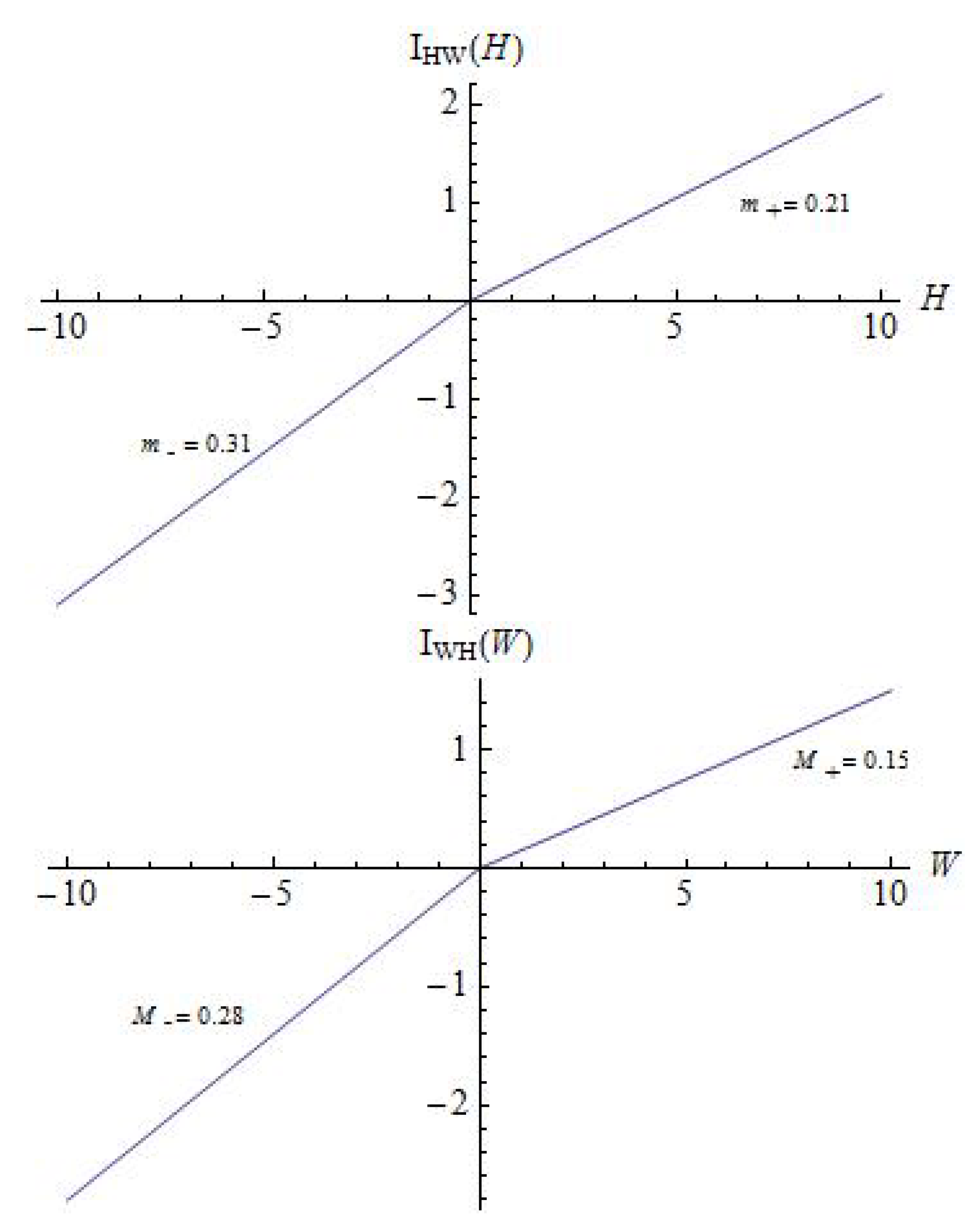
We study the effect of four types of influence functions. We will consider only the case when both husband and wife are validating. According to Gottman: “Validators have an influence function that creates an influence towards negativity in a spouse if the partner’s behavior is negative and an influence towards positivity if the partner’s behavior is positive.” In Figure 1, we show an example with the values we will be using in the numerical simulations, which were taken from Reference [7].
We will use as example the values of the inertia terms for husband and wife given in Gottman’s Table 10.1, which are and . Hence, and , both negative. All the other cases that are considered in Reference [7] can be dealt with in a similar way.
Since it has been observed [7] that, for validating couples, when one spouse is unhappy, his or her effect on the other spouse is larger than when he or she is happy, and the values of the slopes for the negative parts are larger than for the positive parts.
The second one consists of piece-wise constant functions, just like the ojive function of Reference [7]:
are constants that define the influence function of the wife on the husband, and are constants that define the influence function of the husband on the wife. In the analysis done in Reference [7], these functions are non-decreasing, and .
In this work, we consider other scenarios based on conversations with a family therapist and on specific cases studied by Gottman, where is better fitted with more general functions and not necessarily bilinear or piece-wise constant. For instance, we assume , which means that small values of the happiness of one spouse do not affect the other spouse’s happiness. We also study the possibility that, for larger values of the satisfaction (or dissatisfaction), there may be a saturation effect, and the influence function decreases or even goes to zero. The corresponding nullclines can be seen in Figure 2, Figure 3 and Figure 4.
We introduce a third type of influence function where we assume that, for small values of the partner’s satisfaction, the person’s satisfaction increases with a linear rate up to a point and then the rate decreases linearly until, for a certain value, the rate is zero, and similarly for negative values of the satisfaction. In this way, we introduce a saturation of the influence of one spouse on the other. The influence functions are:
The final type of influence functions that we consider are similar to those of the third type only replacing the piece-wise linear functions by piece-wise cubic functions so that the influence functions will not only be continuous but also smooth.
Graphs for these types of influence functions for fixed values of the parameters are given in Section 3. The values of the parameters we chose for all the new influence functions are only academic; they are not based on actual experiments with couples.
1.2. Stochastic Model
The satisfaction or happiness of an individual depends not only on the personality of the person and his or her spouse but also on economic factors, weather, family, political situation, and many other factors. These factors are very hard to quantify and have a large degree of variability and uncertainty. One way to include them in mathematical models is by using Ito Stochastic Differential Equations [9,10].
A class of frequently used stochastic processes is the Brownian one.
We will add a white noise term to our deterministic models.
Here, and are Brownian motions also known in Mathematics as Wiener Processes. Since we assume that the noise does not depend on either spouse’s satisfaction, we are adding the white noise multiplied by a constant or .
2. Analysis of the Deterministic Case
In this section, we study the steady or equilibrium solutions of Equation (4) and their local stability for the four types of influence functions considered. The equilibrium solutions are found by determining the intersection of the nullclines of (4). The local stability of an equilibrium point is found by linearizing (4) around the equilibrium point and finding the eigenvalues of the Jacobian matrix. If all the eigenvalues have negative real part, then the equilibrium point is locally stable. Equilibrium points represent the state of happiness (if the equilibrium point is positive) or unhappiness (if the equilibrium point is negative) the married couple tends to approach.
Qualitative Analysis for the Bilinear Influence Function
These functions define different systems, depending on the quadrant.
The equilibrium points for each case, , can be written as:
where the values of m and M are taken, according to the quadrant under consideration, to be or and or .
If the value of is positive, it means the wife (or husband) is happy. If is negative, it means the wife (or husband) is unhappy. Therefore, if the equilibrium point is in the first quadrant, then both wife and husband are happy. In the third quadrant, both are unhappy. In the second quadrant, the husband is unhappy, and the wife is happy; and, in the fourth quadrant, the wife is unhappy, and the husband is happy.
As usual, the stability of the equilibria is analyzed by linearizing the system around the equilibrium points. The corresponding Jacobians of the linearized system are:
Therefore, , which is negative for the given r’s, ; then, the discriminant is , and the eigenvalues are
Therefore, the critical point of the linearized system will be:
- (1)
- A saddle point if:
- (2)
- A node if:It will be stable if or unstable if .
- (3)
- A spiral if:it will be stable if and unstable if .
- (4)
- A center if:
- (5)
- A proper or improper node if:
It is known (Hartman-Grobman Theorem) that the fixed points of the non-linear system and of its linearization will be of the same kind except when the eigenvalues have a real part equal to zero.
For the problem under investigation, we have , and, for the validating model, always; therefore, and, using the above results, we have proved the following:
Theorem 1.
The equilibrium points, or steady states of system (4) for the bilinear influence function, are given by
for the appropriate values of m and M on the corresponding quadrant. These points are:
- (i)
- Saddle points (and therefore unstable) if and only if , and or
- (ii)
- Stable nodes if and only if and .
It is interesting to note that, while the stability of the equilibrium points (or steady state solutions) depends on the emotional inertia ( and ) and the influence function (m and M), their existence depends also on the values of the individual constants and , which are proportional to the uninfluenced equilibrium points. For the influence function of the bilinear type, it was discovered that, changing only the slopes m and M, the equilibrium points will move around the quadrants, and their stability will also change. This means that, by changing only the influence functions, the satisfaction of the couple can approach a constant value favorable to both if is in quadrant (I), favorable only to the wife if is in quadrant (II), unfavorable to both if is in quadrant (III), and favorable only to the husband if is in quadrant (IV). These steady state solutions can be stable or unstable. If , the satisfaction of the couple will not change with time; otherwise, it will and can get very far from the values . If we are given fixed values for the r’s and the a’s, varying the values of the slopes m and M, we can control the position and stability of the equilibrium states. The same is true if the r’s and the slopes are given; then, varying the a’s, stability and position are determined.
In terms of therapeutic interventions, this describes the situation when, without changing each person (the a’s and the r’s), the satisfaction of the couple can be changed by working jointly with both members to modify the values of the interaction (bilinear influence function), or, when working with husband and wife separately, their uninfluenced equilibrium points (the a’s) are changed. On the other hand, the stability of the equilibria can only be altered by changing the relationship between the inertia, and , and the slopes .
To illustrate the above, we take the values for the variables of the model given in Table 10.1 from Gottman for the validating couple, which are: Inertia for the husband = , and inertia for the wife = ; therefore, We chose influence functions with . Then, the Jacobians have the form:
where the values of the slopes depend on the quadrant. For the first quadrant: . The equilibrium points are
and
then, from Theorem 1, the equilibrium points, if they exist, are stable nodes.
Conditions for the existence of equilibrium points in the first quadrant are and , which mean:
Similar analyses can be carried out for the other quadrants, which will end up in inequalities between the a’s. In this particular example, for all quadrants, and ; therefore, Theorem 1 implies that all the equilibrium points are stable nodes.
Note that, for general validating personality types, and are both negative, so one of the eigenvalues is negative, but the second one may be positive for large enough values of the radicand. This is consistent with Theorem 1.
For the case of influence functions given by piece-wise constants (11) and (12), the number and values of the equilibrium points depend on the values of the constants, but all equilibrium points have the same local stability.
Theorem 2.
The proof is straightforward since the influence functions only add a constant to each equation, and the partial derivatives with respect to H and W are zero, except at the jumps.
Therefore, the Jacobian matrix is
with eigenvalues , and both are negative for validating personalities.
For the other types of influence functions studied, due to the complexity, we will only give the equilibrium points and their stability for fixed values of the parameters. This will be done in the next section.
3. Numerical Simulations
Numerical calculations were done to both validate the theoretical results of the previous section and to find the equilibria and stability for the cases when the analytical solutions are very complicated to find. Particular solutions are also calculated. As mentioned before, we only consider validating personality types since our main objective is to show that the influence functions used have a determining effect on the number of equilibrium points and on their stability and that the same is true of the stochasticity. A similar study can be done for other personality types. The equilibrium points and their stability were found using Mathematica. The simulations of (4) are done using the numerical routine lsode [11], as implemented in Octave. The stochastic system (17) is discretized using Milstein method [9,12].
We are not doing a complete statistical study of the effects of the noise but only including a few representative realizations which show that external influences sometimes do not change very much the state of the system, but sometimes noise can switch the system to a neighborhood of another equilibrium point, with different values for the satisfaction of the couple.
3.1. Single Individual with Validating Personality
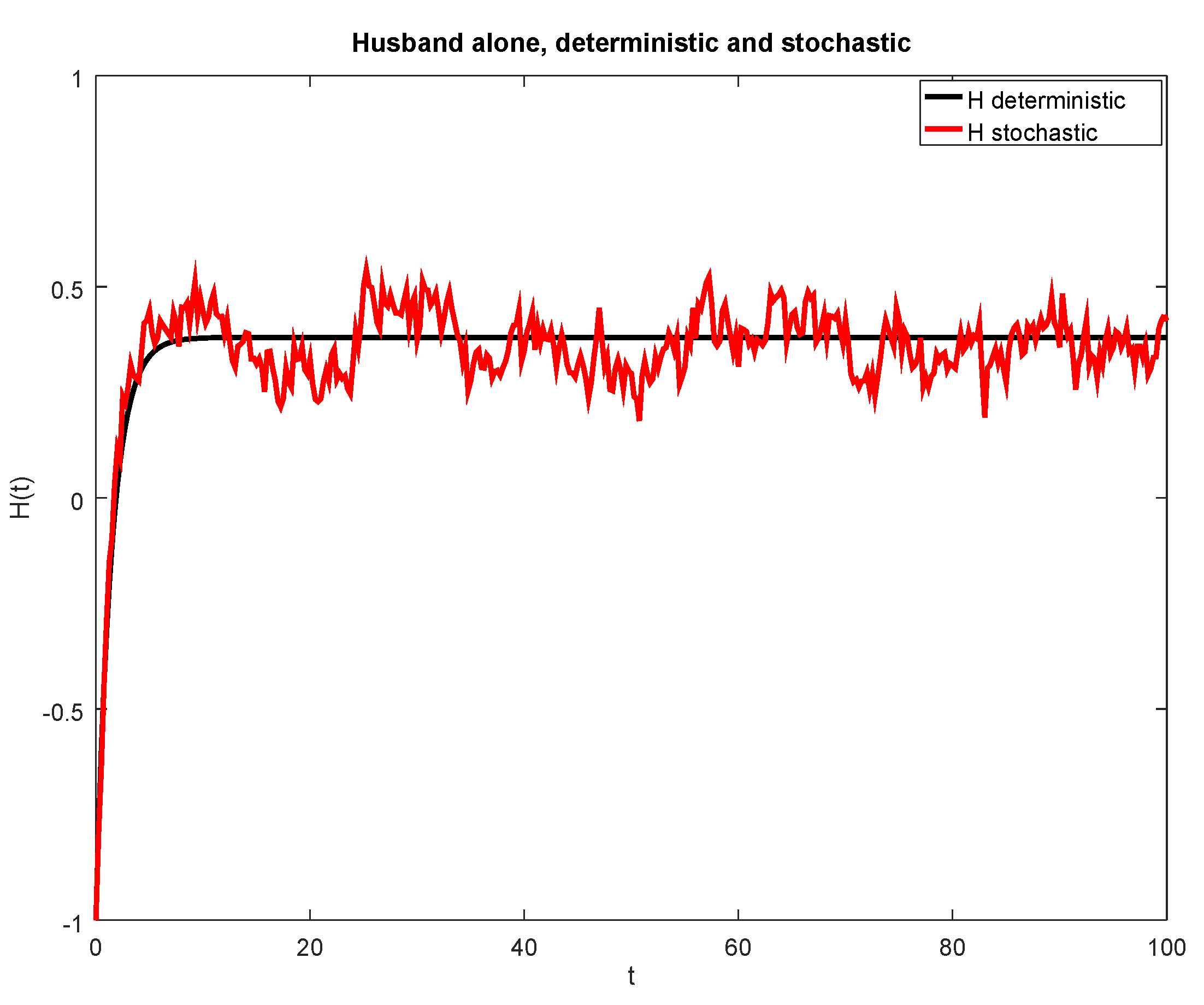
First, consider a single individual with validating personality with no external noise. The values of the parameters are chosen to give the same single equilibrium point given by Reference [7]. These are , which give the uninfluenced equilibrium value of 0.38 for the husband, and giving an equilibrium of 0.52 for the wife. Since the eigenvalues are and , both uninfluenced equilibrium points are stable. Figure 5 is a simulation of the deterministic and stochastic models for the husband without influence from the wife. For the wife, we get a similar plot. The stochastic simulations were done with .
3.2. Validating Wife and Husband with Bilinear Influence Function
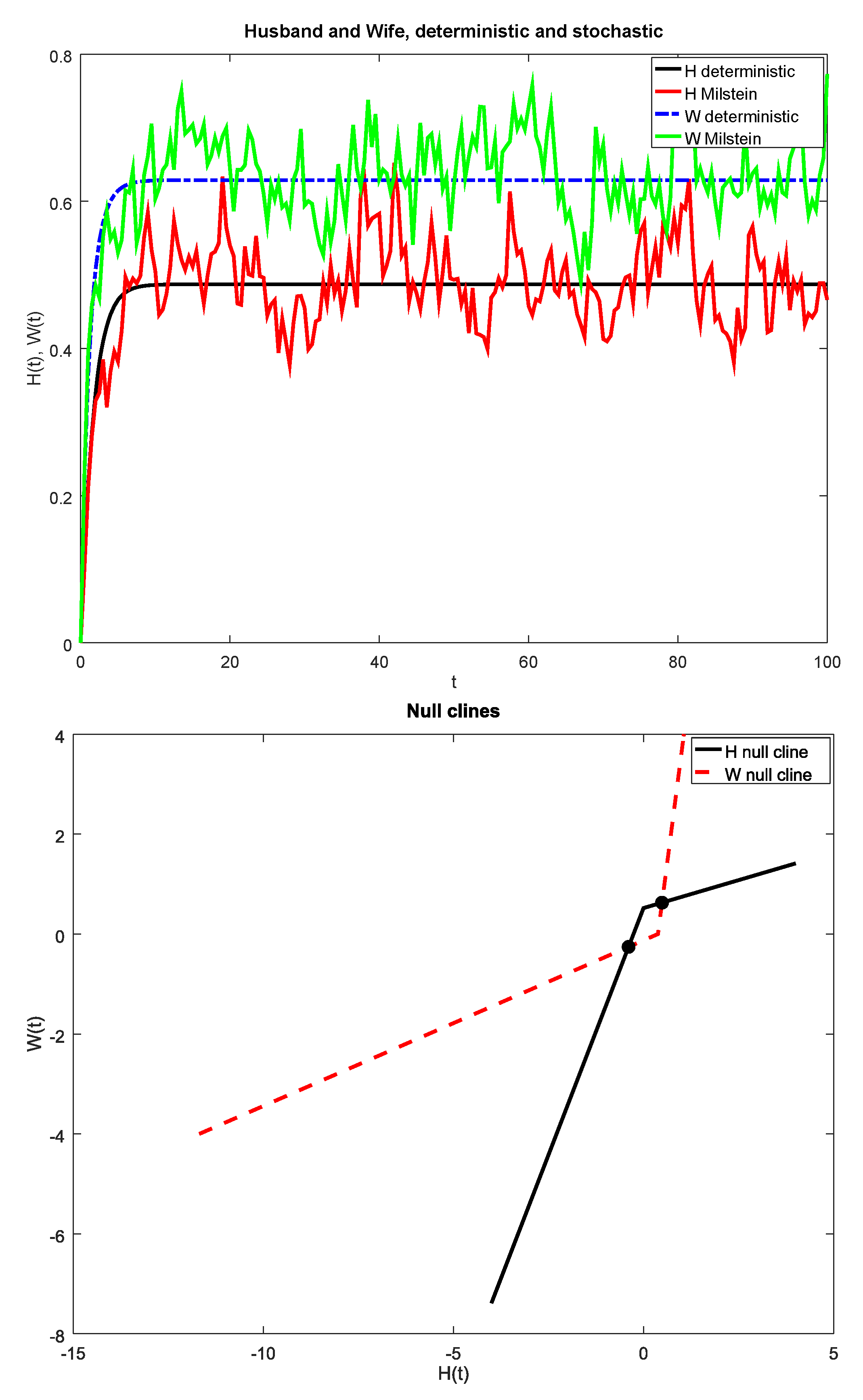
Next, we consider the influence of the spouse. The simplest case is that of bilinear influence functions (9) and (10). The assumption is that, the greater the happiness, the more influence it has on the spouse. For positive values of the happiness, we used the values given by Reference [7]: , . The values of the slopes for negative happiness were just chosen to be larger than the ones corresponding to positive happiness, as stated by Reference [7]. The equilibrium states are , and , . The corresponding eigenvalues are , and , so the positive equilibrium is stable, and the negative unstable. Figure 6 has a simulation for both the deterministic model and a realization for the stochastic one (top) and a plot of the nullclines showing the points of intersection (bottom). The nullclines are obtained from Equation (4). Setting the first equation equal to zero, we obtain
therefore, one nullcline is given by
Similarly, the other nullcline is given by
Observe that the nullclines are rescaled and displaced versions of the influence functions.
3.3. Piece-Wise Influence Function
We will use the same values of , and in all our examples. In addition, in all the following examples, we will only consider that and will call both of them just for simplicity, with or .
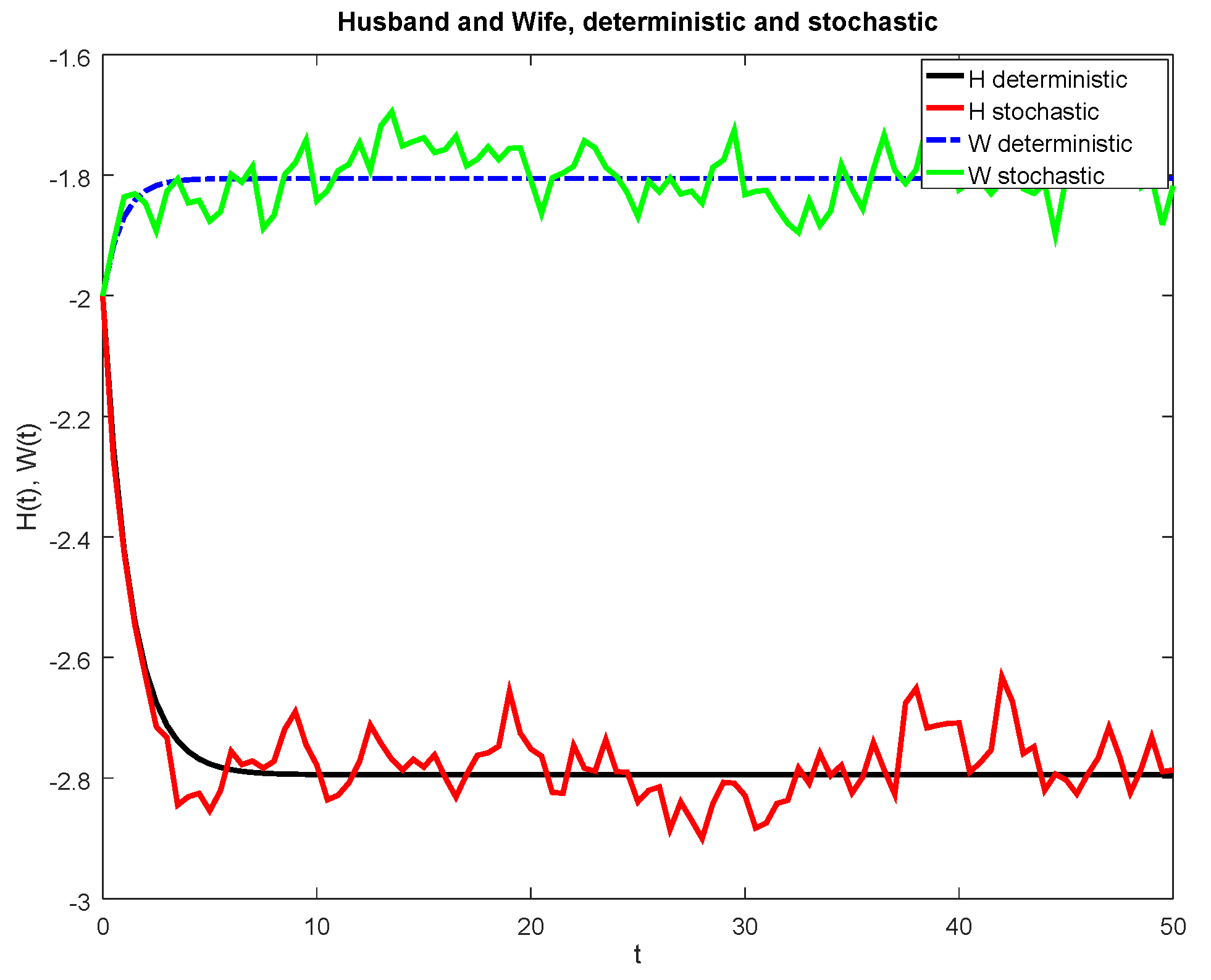
For piece-wise constant influence functions (11) and (12), we studied three different scenarios. Scenario 1 is the case studied by Reference [7], in which the functions are non-decreasing and, as happiness increases, the influence function increases. The values used are , , , , , , For these values, there are three equilibrium points: , (, , and . The eigenvalues for the three are , so all the equilibrium points are stable. Figure 2 has a simulation for both the deterministic model and a realization for the stochastic one (top) and a plot of the nullclines showing the points of intersection (bottom).
Scenario 2 is similar to scenario 1, except that we consider that there is a region around zero satisfaction for which there is no influence on the spouse. The values of the parameters used are , , , , , , , There are now four equilibrium points, , and . The eigenvalues are the same as for scenario 1, and all equilibrium points are still stable. Figure 3 has a simulation for both the deterministic model and a realization for the stochastic one (left) and a plot of the nullclines showing the points of intersection (right).
In scenario 3, we take scenario 2, but, instead of using non-decreasing influence functions, we assume that there is a saturation. For large absolute values of the satisfaction, the person pays less attention to the spouse, and their own satisfaction changes slower or even stops changing. Here, we assume that it stops changing. The values of the parameters are , , , , , , , There are now only two equilibrium points, and . The eigenvalues are the same as for scenario 1, and all equilibrium points are still stable. Figure 4 has a simulation for both the deterministic model and a realization for the stochastic one (top) and a plot of the nullclines showing the points of intersection (bottom).
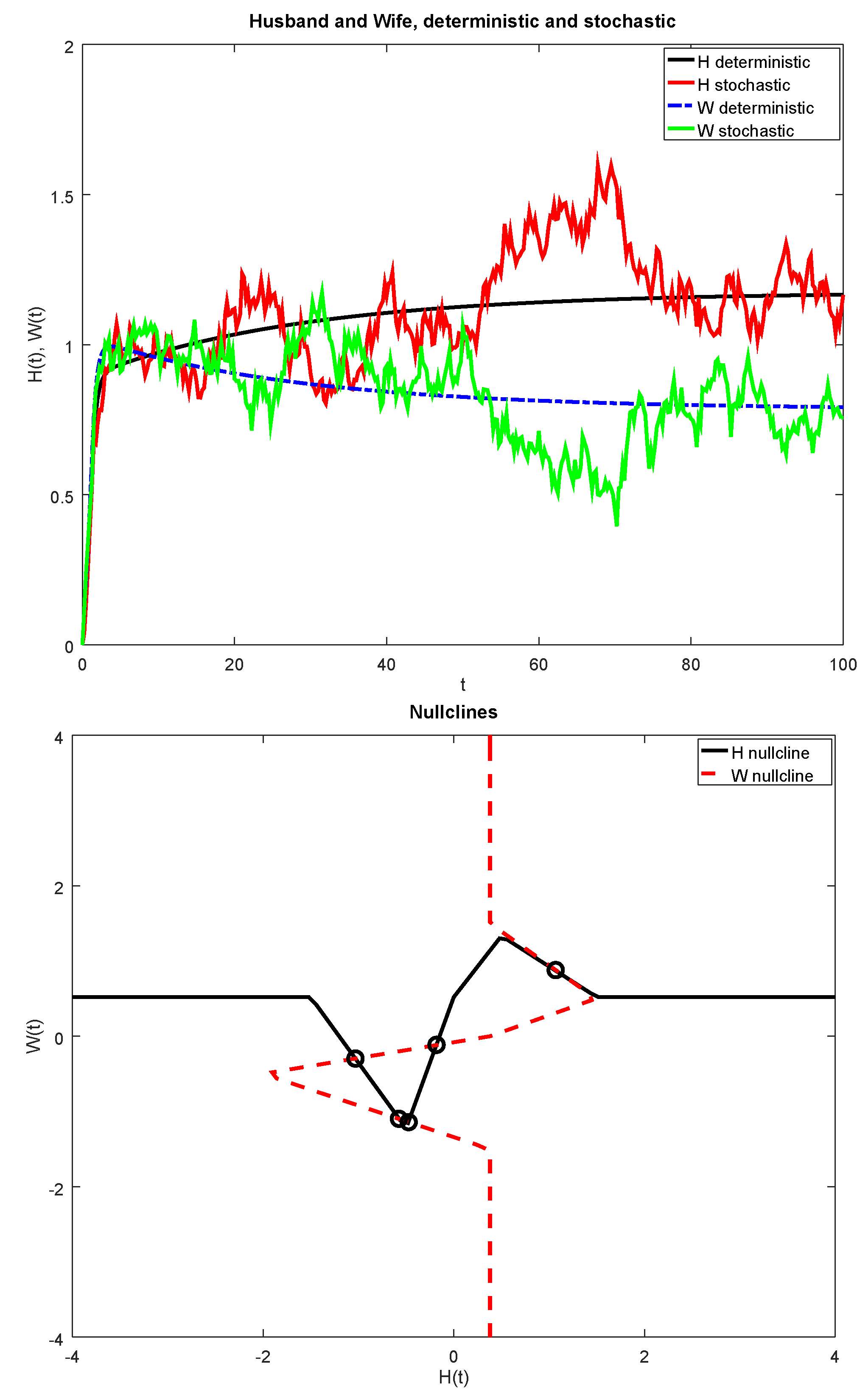
3.4. Piece-Wise Linear Influence Function
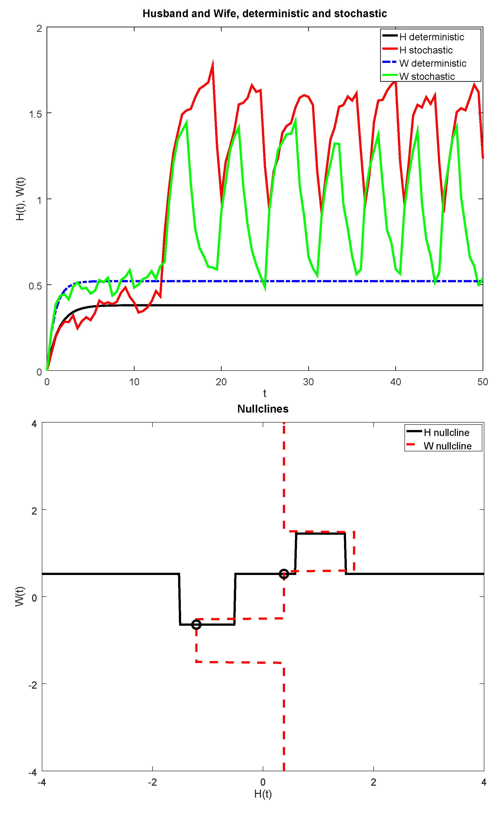
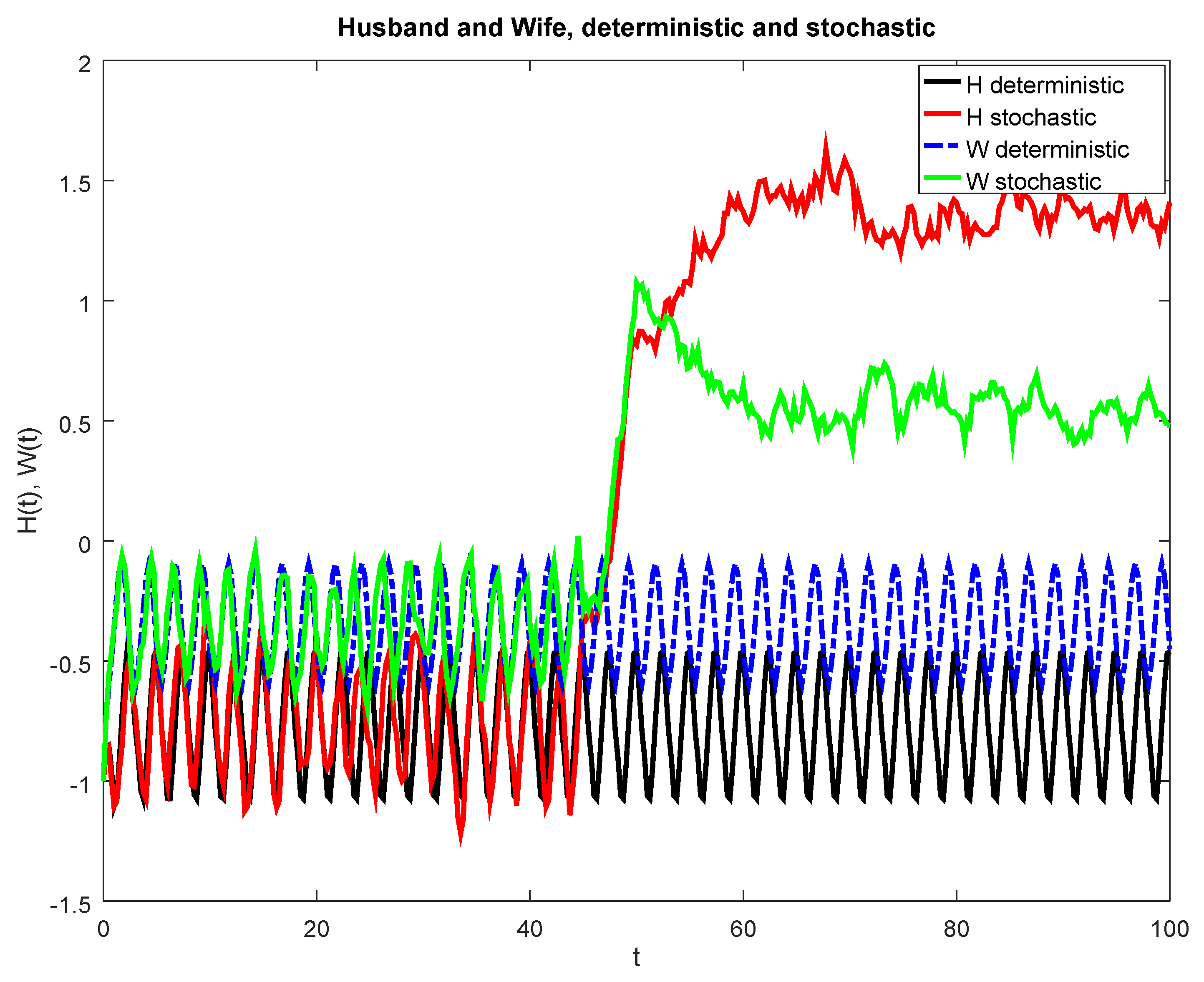
The next influence function we consider is a continuous function formed by piece-wise linear functions. For small positive values of the satisfaction, the influence grows linearly up to a point where its starts to decrease linearly and then goes to zero, and similarly for negative values of the satisfaction. The parameters used in the simulations are , , ; , , There are five equilibrium points, , , , , and . For these equilibrium points, the first, third, and fifth are stable, and the other two unstable. Figure 7 has a simulation for both the deterministic model and a realization for the stochastic one with initial values (top) and a plot of the nullclines showing the points of intersection (bottom).
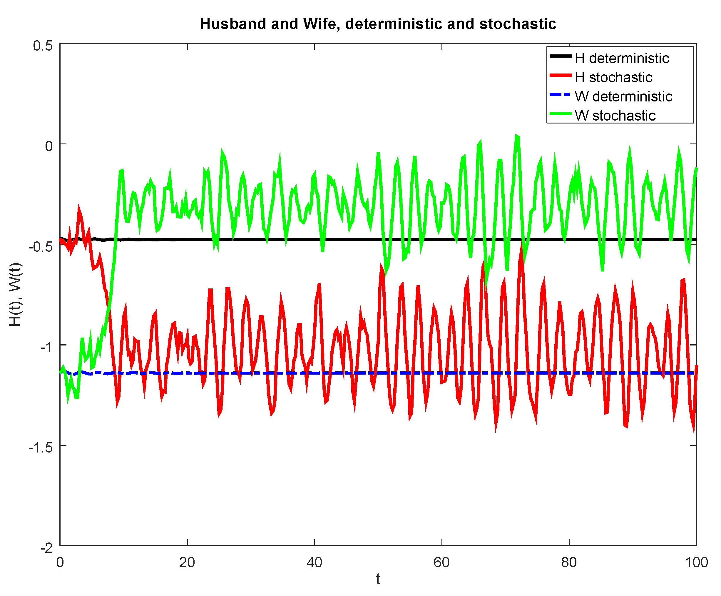
Figure 8 shows a simulation for both the deterministic model and a realization for the stochastic one with initial values . Note that the stochastic solution moves around a different equilibrium point than the deterministic solution. This illustrates that, in certain situations, it is possible for external factors to change the satisfaction of the couple.
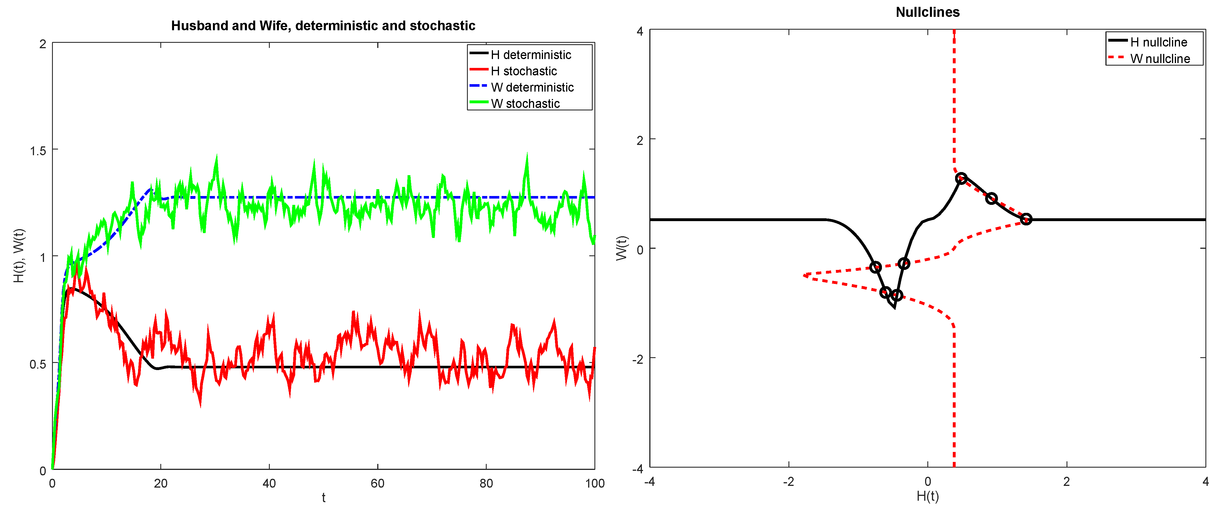
The last influence function used in the examples is a piece-wise cubic, continuous and differentiable everywhere. For small positive values of the satisfaction, the influence grows as a cubic, up to a point where its starts to also decrease as a cubic and then goes to zero, and similarly for negative values of the satisfaction. The parameters used in the simulations are , , ;, , There are seven equilibrium points, , and . The first, third, fifth, and seventh are stable, and the other three unstable. Figure 9 has a simulation for both the deterministic model and a realization for the stochastic one with initial values (left) and a plot of the nullclines showing the points of intersection (right).
Figure 10 shows a simulation for both the deterministic model and a realization for the stochastic one with initial values . Note that the deterministic solution oscillates between two equilibrium points and that the stochastic solution moves around a different equilibrium point. This illustrates that, in certain situations, it is possible to have periodic deterministic solutions and also for external factors to change the satisfaction of the couple.
4. Conclusions
The type of influence functions used in modeling the satisfaction of a couple has a critical influence on the type of solutions obtained. Even the two types of influence functions considered in Reference [7] produce different number of equilibrium points. This suggests that there is a need for determining those functions more accurately. In addition, external factors, such as economic situation, weather, family, and also more drastic ones, such as illness or a death, unemployment, or getting a better job, can change the satisfaction of a couple. We mostly did concrete examples for a type of personalty, but similar results should happen for different influence functions, parameter values, and personality types.
The analysis of the deterministic model led us to unravel the role of the parameters of the models. While the stability of the equilibrium points (or steady state solutions) depends on the emotional inertia and ) and the influence function (m and M), their existence and position depends also on the values of the individual constants and . In therapeutic terms, this means that the position of the steady states can be changed by giving therapy separately to husband and wife, but the stability can only be changed by modifying the interaction of the couple.
The study of the stochastic model showed that some perturbations have very little effect on the satisfaction of the couple, but some can move the couple from one steady state to another or to an oscillatory solution. In other words, the introduction of random external effects can sometimes change the satisfaction of the couple, even when the personalities and type of interaction remain unchanged. In our numerical experiments, roughly 20% of cases led to a qualitative change. This is related to the relative sizes of the white noise and the basins of attraction of the different equilibrium points.
For ease of reference, we include, in Table 1, a summary of the data for the numerical results.
Author Contributions
Conceptualization, B.C.-C., C.E.G.-H. and M.d.C.J.; methodology, B.C.-C., C.E.G.-H. and M.d.C.J.; software, B.C.-C., C.E.G.-H. and M.d.C.J.; validation, B.C.-C., C.E.G.-H. and M.d.C.J.; formal analysis, B.C.-C., C.E.G.-H. and M.d.C.J.; investigation, B.C.-C., C.E.G.-H. and M.d.C.J.; resources, B.C.-C., C.E.G.-H. and M.d.C.J.; data curation, B.C.-C., C.E.G.-H. and M.d.C.J.; writing—original draft preparation, B.C.-C., C.E.G.-H. and M.d.C.J.; writing—review and editing, B.C.-C., C.E.G.-H. and M.d.C.J.; visualization, B.C.-C., C.E.G.-H. and M.d.C.J.; supervision, B.C.-C., C.E.G.-H. and M.d.C.J.; project administration, B.C.-C., C.E.G.-H. and M.d.C.J. All authors have read and agreed to the published version of the manuscript.
Funding
This research received no external funding.
Acknowledgments
We thank Ramiro Chavez and Ana Perez for their computational support and the reviewers for their very pertinent comments.
Conflicts of Interest
The authors declare no conflict of interest.
References
- Strogatz, S.H. Nonlinear Dynamics and Chaos with Student Solutions Manual: With Applications to Physics, Biology, Chemistry, and Engineering; CRC Press: Boca Raton, FL, USA, 2018. [Google Scholar]
- Elishakoff, I. Differential Equations of Love and Love of Differential Equations. J. Humanist. Math. 2019, 9, 226–246. [Google Scholar] [CrossRef] [Green Version]
- Ghosh, K. Love between Two Individuals in a Romantic Relationship: A Newly Proposed Mathematical Model. In Proceedings of the 7th IMT-GT International Conference on Mathematics, Statistics and Its Applications, Bangkok, Thailand, 21–23 July 2011; Volume 21. [Google Scholar]
- Rey, J.M. A mathematical model of sentimental dynamics accounting for marital dissolution. PLoS ONE 2010, 5, e9881. [Google Scholar] [CrossRef] [PubMed] [Green Version]
- Binder, P.M. Chaos and Love Affairs. Math. Mag. 2000, 73, 235–236. [Google Scholar] [CrossRef]
- Gragnini, A.; Rinaldi, S.; Feichtlinger, G. Cyclic Dynamics in Romantic Relationships. Int. J. Bifurc. Chaos 1997, 7, 2611–2619. [Google Scholar] [CrossRef]
- Gottman, J.M. The Mathematics of Marriage: Dynamic Nonlinear Models; MIT Press: Cambridge, MA, USA, 2005. [Google Scholar]
- Allen, L.J. Introduction to Mathematical Biology; Pearson/Prentice Hall: Upper Saddle River, NJ, USA, 2007. [Google Scholar]
- Evans, L.C. An Introduction to Stochastic Differential Equations; American Mathematical Society: Providence, RI, USA, 2012; Volume 82. [Google Scholar]
- Allen, E. Modeling with Itô Stochastic Differential Equations; Springer Science & Business Media: Berlin, Germany, 2007; Volume 22. [Google Scholar]
- Hindmarsh, A.C. Ordinary Differential Equation System Solver; Technical Report; Lawrence Livermore National Laboratory: Livermore, CA, USA, 1992. [Google Scholar]
- Kloeden, P.; Platen, E. Applications of mathematics. In Numerical Solution of Stochastic Differential Equations; Springer: Berlin, Germany, 1992; Volume 23. [Google Scholar]
Figure 1.
Bilinear influence functions (top) and (bottom).

Figure 2.
Piece-wise constant influence functions, scenario 1. Plot of H and W vs. time for the deterministic case and a stochastic realization (top) and a plot of the nullclines and the equilibrium points (bottom). Observe that these nullclines are discontinuous; therefore, for the H nullcline only, the horizontal lines count, and, for the W nullcline, only the vertical parts count.

Figure 3.
Piece-wise constant influence functions, scenario 2. Plot of H and W vs. time for the deterministic case and a stochastic realization (top) and a plot of the nullclines and the equilibrium points (bottom).
Figure 3.
Piece-wise constant influence functions, scenario 2. Plot of H and W vs. time for the deterministic case and a stochastic realization (top) and a plot of the nullclines and the equilibrium points (bottom).


Figure 4.
Piece-wise constant influence functions, scenario 2. Plot of H and W vs. time for the deterministic case and a stochastic realization (top) and a plot of the nullclines and the equilibrium points (bottom). In this example, the external white noise significantly changes the state of satisfaction of the couple.

Figure 5.
A numerical simulation of the deterministic case and a stochastic realization for a validating husband with no influence from the wife.
Figure 5.
A numerical simulation of the deterministic case and a stochastic realization for a validating husband with no influence from the wife.

Figure 6.
Bilinear influence functions. Plot of H and W vs. time for the deterministic case and a stochastic realization (top) and a plot of the nullclines and the equilibrium points (bottom). In this example, the external noise only makes the satisfaction oscillate around the equilibrium state of the deterministic case.

Figure 7.
Piece-wise linear influence functions. Plot of H and W vs. time for the deterministic case and a stochastic realization with initial values (top) and a plot of the nullclines and the equilibrium points (bottom).
Figure 7.
Piece-wise linear influence functions. Plot of H and W vs. time for the deterministic case and a stochastic realization with initial values (top) and a plot of the nullclines and the equilibrium points (bottom).

Figure 8.
Piecewise linear influence functions. Plot of H and W vs. time for the deterministic case and a stochastic realization with initial values .
Figure 8.
Piecewise linear influence functions. Plot of H and W vs. time for the deterministic case and a stochastic realization with initial values .

Figure 9.
Piece-wise cubic influence functions. Plot of H and W vs. time for the deterministic case and a stochastic realization with initial values (left) and a plot of the nullclines and the equilibrium points (right).
Figure 9.
Piece-wise cubic influence functions. Plot of H and W vs. time for the deterministic case and a stochastic realization with initial values (left) and a plot of the nullclines and the equilibrium points (right).

Figure 10.
Piece-wise cubic influence functions. Plot of H and W vs. time for the deterministic case and a stochastic realization with initial values .
Figure 10.
Piece-wise cubic influence functions. Plot of H and W vs. time for the deterministic case and a stochastic realization with initial values .


Table 1.
Summary of parameter values used. The same values for , and are used in all our examples.
| Figure Number | Type of Influence Function | Parameters |
|---|---|---|
| 2 | Zero influence function | , . |
| 3 | Bilinear | , , , , ; , , . |
| 4 | Piece-wise constant | , , , , , , |
| 5 | Piece-wise constant | , , , , , , , |
| 6 | Piece-wise constant with saturation | , , , , , , , |
| 7 and 8 | Piece-wise linear | , , ; , , |
| 9 and 10 | Piece-wise cubic | , , ; , , |
Publisher’s Note: MDPI stays neutral with regard to jurisdictional claims in published maps and institutional affiliations. |
© 2020 by the authors. Licensee MDPI, Basel, Switzerland. This article is an open access article distributed under the terms and conditions of the Creative Commons Attribution (CC BY) license (http://creativecommons.org/licenses/by/4.0/).
Share and Cite
MDPI and ACS Style
Chen-Charpentier, B.; Garza-Hume, C.E.; Jorge, M.d.C. A Continuous Model of Marital Relations with Stochastic Differential Equations. Math. Comput. Appl. 2021, 26, 3. https://0-doi-org.brum.beds.ac.uk/10.3390/mca26010003
AMA Style
Chen-Charpentier B, Garza-Hume CE, Jorge MdC. A Continuous Model of Marital Relations with Stochastic Differential Equations. Mathematical and Computational Applications. 2021; 26(1):3. https://0-doi-org.brum.beds.ac.uk/10.3390/mca26010003
Chicago/Turabian StyleChen-Charpentier, Benito, Clara Eugenia Garza-Hume, and María del Carmen Jorge. 2021. "A Continuous Model of Marital Relations with Stochastic Differential Equations" Mathematical and Computational Applications 26, no. 1: 3. https://0-doi-org.brum.beds.ac.uk/10.3390/mca26010003