Estimating the Market Share for New Products with a Split Questionnaire Survey


Geneva School of Business Administration, University of Applied Sciences and Arts Western Switzerland (HES-SO), Rue de la Tambourine 17, 1227 Carouge, Switzerland
*
Author to whom correspondence should be addressed.
Math. Comput. Appl. 2021, 26(1), 7; https://0-doi-org.brum.beds.ac.uk/10.3390/mca26010007
Submission received: 13 November 2020
/
Revised: 23 December 2020
/
Accepted: 6 January 2021
/
Published: 9 January 2021
(This article belongs to the Section Social Sciences)
Abstract
:When designing a new product, conjoint analysis is a powerful tool to estimate the perceived value of the prospects. However, it has a drawback: when the product has too many attributes and levels, it may be difficult to administrate the survey to respondents because they will be overwhelmed by the too numerous questions. In this paper, we propose an alternative approach that permits us to bypass this problem. Contrary to conjoint analysis, which estimates respondents’ utility functions, our approach directly estimates market shares. This enables us to split the questionnaire among respondents and, therefore, to reduce the burden on each respondent as much as desired. However, this new method has two weaknesses that conjoint analysis does not have: first, inferences on a single respondent cannot be made; second, the competition’s product profiles have to be known before administrating the survey. Therefore, our method has to be used when traditional methods are less easily implementable, i.e., when the number of attributes and levels is large.
JEL Classification:
C830; C900; M3101. Introduction
Starting from the seminal work of Green and Rao [1], conjoint analysis has become a central tool for the study of marketing problems involving multiattribute alternatives (see [2,3,4,5,6,7,8,9] for some article reviews). Conjoint analysis is a method used in market research to estimate how people value the different attributes of a product. The term attribute refers to a characteristic of a product (e.g., colour) which can take different values (e.g., blue, red, green) also named attribute’s levels. Using a survey where respondents have to state their preference among different potential products, it is possible to estimate with regressions techniques the implicit value of each single attribute’s level. These implicit values, known as part-worths or utilities, can be used to estimate, for example, market share or revenue of a new product. Ordinary least squares (OLS) regression has been among the most widely used techniques in conjoint analysis to reconstruct the individual utility from the survey data [5,10,11]. In this case, data can be collected in the form of ratings or pseudo-interval-scaled rankings (the robustness of the latter option being shown by [11] and discussed, for instance, by [12]).
The problem of dealing with a large number of attributes and levels has always been among the main issues in conjoint analysis. Among the principal difficulties, we may distinguish two (however partially related) aspects. First, if too many profiles have to be ranked or rated, then the respondent may be unable to provide accurate estimations. The number of experimental profiles can be reduced by employing fractional factorial designs and orthogonal plans [13], or by using an algorithmic construction to pursue some optimality criteria (such as D-optimality), which allows for more flexibility in the choice of the number of profiles. However, the usage of OLS regression imposes a lower limit in the design size, since it requires the number of profiles to be larger than the total number of parameters. Unfortunately, this leads to problematic situations for many real case studies. Second, a product described by too many attributes may confuse the respondent, which could therefore assess a wrong judgement on the product’s utility. Over the last few decades, many methods have been proposed to overcome both of these problems. For example, Green [13] suggested to employ “partial profiles”, i.e., to only display subsets of the attributes (as opposite to the “full-profile” approach). Another way to accommodate a large number of attributes is to use a so-called bridging design that enables one to split up the attributes and levels in two different lists that are bridged with common attributes (see for instance [14] for an application). A further simplification was introduced with the concept of hybrid models [15,16], where a (possibly “partial-profile”) conjoint measurement is preceded by a “self-explicated” step. Other developments led to the use of Bayesian methods [17,18] to estimate the missing data and reconstruct the complete utility function at the individual level. See also [19] for an early review of hybrid models, and [20] for a more recent Bayesian model.
In parallel to the lineage to which Green, among others, has given his main contribution, other methods have been developed. A trade-off approach was proposed by Johnson [21], according to which the respondent is requested to state her own preference about particular levels of one attribute compared to another. This approach offers an alternative way of tackling the problems due to the large number of attributes, although the price to pay may be some loss in realism [12]. In the 1980s, further developments of Johnson’s trade off approach led to a more complex method, known as Adaptive Conjoint Analysis (ACA). This analysis is performed on a software which, as suggested by the name, gradually adapts the questions to be administered as the data are being collected. In the 1980s, Choice-Based Conjoint Analysis started to become popular. In particular, a choice-based approach proposed and developed by Louviere and others [22,23] is now among the most relevant methods in conjoint analysis. In this case, to simulate a more realistic market environment, the respondent has to make a choice among alternatives instead of providing rankings or ratings. Choice models, such as the multinomial logit model, are employed to analyze data that are collected in such a way (see for instance [24] for more details). Despite the large variety of conjoint analysis techniques that have emerged throughout the years, the problem of handling a large number of attributes—which has been emphasized by [5] and, later, by [7,9,25] as one of the most urgent tasks for the future development—has not yet found a fully satisfying answer. More recent progress on this issue has been made by developing adaptive choice-based conjoint [26], or hybrid and self-explicated methods [27,28,29,30,31].
In some studies, Monte Carlo methods have been used to assess the accuracy and the robustness of conjoint analysis. Carmone et al. [11] seem to be the first to investigate the efficiency of conjoint analysis methods using Monte Carlo simulations. To measure the efficiency, they took the correlation between the real part worths and their estimation and performed statistical tests using the Fisher z-transformation. A few years later, Wittink and Cattin [32] studied the performance of conjoint analysis using three different criteria, namely: the correlation between the real utility and its estimation, the Kuskal’s stress value and the Pearson rank correlation coefficient. In the 1990s, Vriens et al. [33] compared different metric conjoint segmentation methods using Monte Carlo simulations. They simulated the huge variety of real cases by randomly varying different parameters such as the sample size, the number of segments, the homogeneity in the segment, and so on. In terms of the performance, they employed six different measures, most of them based on the root-mean-square error (RMSE). It is worth mentioning here that this systematic study greatly inspired the design of subsequent Monte Carlo simulations conducted to assess the accuracy of conjoint analysis methods [34,35,36,37,38].
The present paper proposes an alternative approach to conjoint analysis for estimating the market share of a new product. Our method allows estimating the market share even when the number of attributes and levels are large. However, as a main difference with respect to conjoint analysis, our approach does not reconstruct utilities neither at the individual nor at the segment level. Instead, it directly estimates the market share. This enables us to split the questionnaire among respondents and therefore to reduce the burden on each respondent as much as desired. In essence, the proposed method is composed of three steps. The first step consists of designing the split questionnaire. For this purpose, a D-optimal basis is computed from the set of all possible product profiles. Then, for each respondent, a subset of the basis is chosen using a random block algorithm. The survey is conducted in the second step. Roughly speaking, each respondent has to state her preference between each product in the subset and the competition’s products. In the third step, using the stated preferences of each respondent, the share of preference is approximated with a logistic regression. The software provided as Supplementary Materials allows the practitioners to implement the method in a user-friendly way. We notice that other softwares are available for the design of experiments, such as Ngene (which is however not free), and could be used to construct the split questionnaire in a very efficient way. Our software does not have the flexibility of Ngene, but serves for a unique purpose, i.e., the estimation of the share of preference, and integrates in a unique and simple framework both computer-based steps (split questionnaire construction and share of preference estimation) that build up our method. Notice that, by contrast, Ngene does not perform the preference estimation on the basis of the survey data.
Our method fully overcomes the first of the aforementioned problems regarding large numbers of attributes and levels, i.e., the risk of presenting too many profiles to each respondent. In contrast, because we propose to conduct full-profile questionnaire administration, the respondents may still be confused by the complexity of products in the case of very large numbers of attributes and levels. However, notice that the complexity of the products also affects real-world decisions. Because we simply ask respondents to state pairwise preferences, our approach does not deviate too far from the situation in a real market.
To assess the statistical performance of this new approach, we compare it with the popular full-profile conjoint analysis with rank orders and with parth-worths estimated by OLS regression. For this purpose, we conduct Monte Carlo simulations and we show that the accuracy of our method is comparable to that of conjoint analysis. We are aware that more recent conjoint analysis methods would be, in principle, more appropriate to perform a comparison. However, the choice to compare our method with standard, full-profile conjoint analysis is motivated by the aim of keeping the comparison as clean and simple as possibile, so as to better highlight the features of our new method. By contrast, making a direct comparison against hybrid methods would be difficult because of the self-explicated part, which would need ad hoc assumptions to model respondent error. We notice that standard full-profile conjoint analysis has often been recognised as a robust method even when compared with hybrid models (see, e.g., [16]). Moreover, as discussed below, in the simulations performed in this paper we assume no respondent error, and assign to respondents of the conjoint analysis simulations tasks that would be too demanding for a real survey (in particular, we ask each respondent to rank up to 64 different profiles). As a consequence, we expect the performance of full-profile conjoint analysis to be significantly better in our simulations than in a real-case study. We expect therefore that this assumption reduces the gap between the somewhat dated full-profile conjoint analysis and the more recent conjoint models, such as hybrid of choice-based models. We leave for future research further comparisons against more sophisticated approaches (as for instance the methods provided by the Sawtooth software), which address more explicitly the issue of coping with a large number of attributes and levels.
The present paper proposes a new approach to estimate the market share for new products. Thanks to a split questionnaire design, our approach permits us to reduce the burden on each respondent as much as desired and can be used even when the number of attributes and levels is large. The paper is organized as follows. Section 2 summarizes the method we propose for estimating the market share of a new product. Section 3 discusses some variants we considered, and motivates the choices we made. Section 4 exposes the Monte Carlo simulations we use for testing the efficiency of different methods in estimating market shares. In Section 5, we investigate the efficiency of the proposed method. First, we show how it outperforms candidate alternatives. Then, we investigate how the experimental design can be optimized. Subsequently, we compare the efficiency of the proposed method against standard conjoint analysis. Finally, in Section 6, we conclude and indicate further research directions.
2. The Proposed Method
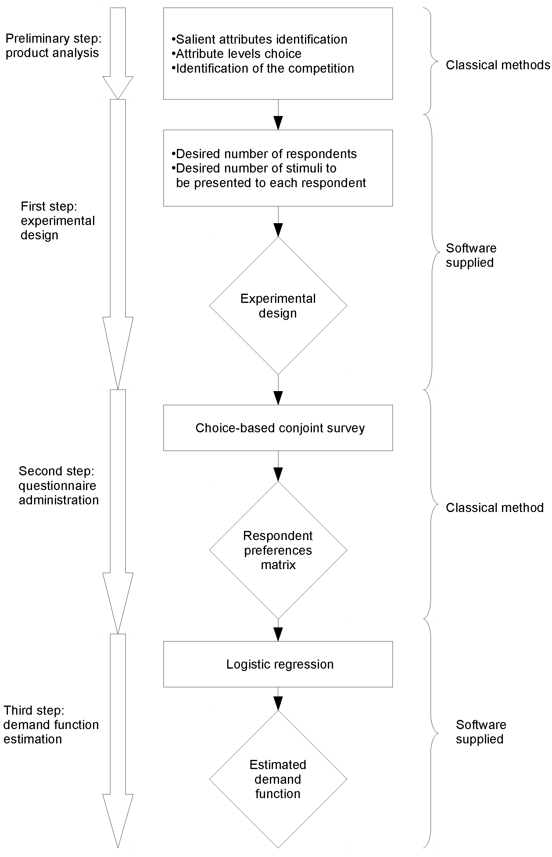
This section presents the method that we propose in this paper. An explanation of the rationale behind the choice of its features among some considered alternatives is left to Section 3 and Section 5. The method consists of three main steps preceded by a preliminary product analysis, which is in turn composed of three tasks. (see Figure 1).
In the preliminary analysis, we first identify the salient attributes of the product. This can be achieved by using classical methods; for instance, a semi-structured interview followed by a self-explicated conjoint analysis will be perfectly adequate. The second task consists of choosing, for each salient attribute, the levels to be considered. The last task requires to identify the products that are proposed by the competition.
We will now describe the three main steps building the method, namely: the construction of the experimental design, the questionnaire administration and the estimation of the demand function. Please note that for the sake of clarity, we begin with the second step.
2.1. Questionnaire Administration
The aim of the survey is to reveal whether a given product profile is preferred over the products proposed by the competition. The survey relies on a traditional full profile analysis and is composed of two stages. In the first stage, we identify from the products that are proposed by the competition the one that is preferred by the respondent. If the number of products in the competition is too large, then we can proceed with multiple pairwise comparisons rather than a single choice-based analysis. In the second stage, the respondent has to state her preference or indifference between a set of profiles that are presented to her and the preferred competition’s product. This stage consists of a series of pairwise comparisons and it should not be too long because it has to keep the attention of the respondent.
2.2. Experimental Design
We now outline the procedure for selecting the profiles that will be administered to each respondent. Notice that it is beyond the scope of this paper to discuss, by contrast, the methodology for choosing a representative sample of respondents.
Given the salient attributes identified in the preliminary product analysis and the desired split questionnaire size (i.e., the desired number of profiles to be addressed to each respondent and the desired number of respondents to be interviewed), our method constructs a split questionnaire, the size of which stays as close as possible to the desired one. All of the distinct profiles that are found in the split questionnaire form a D-optimal basis. To maximize the performance (as we found with the numerical experiments discussed in Section 5), the number of profiles composing the basis is chosen to be as large as possible, insofar as this is compatible with the questionnaire size. Once the basis has been obtained, a random block algorithm completes the construction of the split questionnaire by assigning to each respondent a subset of the basis profiles. The D-optimal basis is computed with a modified Fedorov algorithm [39] whereas the random block experimental design is constructed with the same algorithm that was used to calculate the starting design in [40].
2.3. Demand Function Estimation
The demand function is estimated by using a logistic function of main effects, the coefficients of which are determined by a logistic regression procedure. The resulting demand function estimation allows the user to predict the market share for every possible product profile, provided that the latter can be described by the attributes and levels that have been identified in the preliminary analysis.
3. Considered Methods
This section summarizes all methods that are taken into account in the present study, and which are tested for efficiency in the Monte Carlo simulations exposed in Section 4 and Section 5.
For the demand function estimation, we consider the following two models:
- Linear function
- Logistic function.
In both cases, we also investigate the two options of modeling main effects alone, or including first-order interactions.
For the regression design, we use D-optimal designs (the choice of D-optimality among other optimality criteria is discussed in Section 3.2).
For what concerns the block experimental design for splitting the questionnaire, we study the following options:
- Random block,
- -optimal,
- A-optimal,
- Homogeneous groups.
The rest of the section motivates these preliminary choices and contains technical points. It can be skipped at first reading.
3.1. Demand Function Model
We consider a family of products with m salient attributes and where the number of possible levels is finite. Let us denote by the attributes and by the number of levels for attribute a. To describe the different product profiles, we use the standard dummy-coding for regression designs. We denote by the column-vector describing the product profile. In this coding, the first element is associated with the intercept of the regression and is equal to 1. Then, the following elements describe the product profile with a binary coding: if the corresponding attribute level is encountered and otherwise. As usual, to avoid collinearity, the levels of attribute a are coded using only binary variables. Consequently, the size of the vector is
As mentioned earlier, two classical options are considered, namely: the logistic and the linear function. Given that the method we propose makes use of the logistic approach, and because the linear approach is well-known, we limit ourselves to the description of the former case. To predict the share of preference for the product profile , we use the logistic model
where is the transpose of the column-vector of inferred parameters . The choice of this function is mainly motivated by the natural way in which it fits the unit interval. As already mentioned, the parameters are estimated using data obtained from a split questionnaire survey. For this purpose, a regression design containing v different profiles is selected. The transposes of these vectors form the design matrix X of size . During the survey, b respondents are interviewed but, because we use a split questionnaire, not all of the profiles are presented to a given respondent. To describe this particularity, we use the following assignation matrix:
where and . We represent the results of the survey through the preference variables
Finally, the estimation of the demand function is achieved by means of a logistic regression. According to the standard logistic regression procedure, the parameter is found by maximizing the log-likelihood
for the variable .
At this point let us make some comments about terms we will use throughout the rest of the paper. We denote as demand function, the logistic function that describes the share of preference for all possible product profiles. We denote as market share the share of preference computed with the logistic function when the product profile is set to a given value.
3.2. Regression Design
In this subsection, we discuss possible ways to construct efficient regression designs. We start by reviewing optimality criteria for linear models, and consider the proper logistic problem only at a second step. Indeed, as discussed later on, our approach to construct efficient designs for logistic regression will borrow the optimality criterion from linear theory.
The methods of experimental designs, first introduced by Fisher see, e.g., [41], soon focused on the problem of constructing fractional factorial experiments [42,43,44,45,46], and in particular on orthogonal designs, which ensure a minimal variance of the estimated parameters in the case of linear regression models, see, e.g., [47]. Later efforts led to catalogues of basic orthogonal plans for a wide variety of cases, see, e.g., [48]. However, in many practical situations, an orthogonal plan cannot be constructed unless the number of levels or plots is enforced to accommodate the design requirements, which may of course imply a loss in the quality of the collected information. Consequently, the problem become central of constructing efficient (or optimal) designs for an arbitrary number of attributes, levels or profiles. As discussed in detail by Kiefer and Wolfowitz [49,50,51], possible criteria to define optimality are based on the eigenvalues of the covariance matrix of the inferred parameter vector . In particular, A-, D- and E-optimality require the trace, the determinant and the maximal eigenvalue of the covariance matrix to be minimal, respectively. Other possible criteria to define optimality are based on the variance of predictions. For instance, the G-optimality requires the maximal variance among all design points of the linear estimator of the regression function to be minimal. An important result obtained by [52] stated the equivalence between D-optimality and G-optimality. This is a strong argument in favor of D-optimality because it is easier to compute than G-optimality. Further motivations are based on the invariance under linear transformations of the D-optimality criterion [49], on the volume minimization of particular confidence regions in parameter space [49,53], or rely on Bayesian arguments [54]. These reasons led us to choose, for linear regression purposes, the D-optimality criterion rather than A- or E-optimality. For algorithmic construction, D-optimality tends to be the preferred method [55]. In the 1970s, the first algorithms to achieve D-optimality were proposed [56,57,58,59]. In particular, Fedorov’s algorithm is among the most important and most widely used methods to achieve D-optimality. A modified Fedorov algorithm, with similar precision but increased speed, was successively proposed by [39] and recommended by [55] for use in conjoint analysis.
The problem of constructing optimal designs for logistic regression (which belongs to the class of generalized linear models) is a rather complex one. In the standard approach, one approximates the variance-covariance matrix of the parameter vector by the inverse of the observed Fisher matrix I, see, e.g., [60]. The main difficulty stems from the fact that, unlike in linear regression, the Fisher matrix I depends on the maximum likelihood estimate , the determination of which is actually the final goal of the regression procedure. More precisely, denoting by the v row vectors of the regression matrix X, the Fisher matrix elements are defined by the expectation value, see, e.g., [61]
where E denotes the expectation value and Y is the random variable describing the consumers’ choice:
One can show that for generalized linear models, the Fisher matrix takes the form
where W is a diagonal “weight” matrix , w being a single-valued function that depends on the model (in the case of a logistic model ). Various proposals have been made to estimate the Fisher matrix, despite the intrinsic difficulties. Chernoff [62] introduced the notion of locally optimal designs, the construction of which requires the parameter vector to be initialized with a prespecified value. Later proposals involved a Bayesian estimation [61,63] that instead makes use of a probability distribution describing prior knowledge of the parameters to be estimated (see [64] for a review of optimal Bayesian designs). However, in the framework of our method, no prior information is assumed to be available. Criteria for the evaluation of Bayesian methods under uninformative priors have been recently discussed, for instance, by [65] (see also the discussion about uniform prior distributions by [66]). Nevertheless, modeling an uninformative prior still requires some assumptions, such as to define interval boundaries for the parameters. Because our method is meant to be used in a wide range of cases, so that it would be difficult to infer a universally valid, though uninformative, prior distribution for the maximum likelihood parameter vector, we prefer to avoid embarking on the construction of Bayesian designs. Opting again for simplicity, we decided to evaluate the Fisher matrix I by prespecifying the “most neutral” parameter vector . In this way, the Fisher information matrix equals, up to a constant factor, the Fisher information matrix for linear regression (i.e., ). Therefore, with this assumption, the problem is reduced to a linear model optimization. Relying on the previous discussion about optimality criteria for linear models, we decided to also adopt D-optimality as the criterion for building the experimental designs for logistic regression purposes. We implemented a modified Fedorov algorithm, according to the prescriptions of [39], and construct D-optimal designs by taking the best result among 100 algorithm runs, each with a different random design initialization.
3.3. Split-Questionnaire Design
Once the profiles composing the D-optimal basis have been selected, the next task is to split them among the different respondents. Let us denote by v the size of the D-optimal basis. The problem can be formulated as follows: v different profiles, each replicated r times, have to be administered to b respondents; then, every respondent is asked to state her preference about different product profiles. In this subsection, we investigate the possible ways of distributing the totality of questions among the b respondents. Identifying each respondent with a block allows us to use the same formalism that is commonly employed in block design theory. Notice that the mathematical problem that we face substantially differs from the one that is typically found in the response of blocked experiments, and we do not expect to have any particular correspondence for what concerns, for instance, the efficiency of the block design.
Consider the number of times where both profiles and are assigned to the same respondent (i.e., fall within the same block). The larger , the stronger will be the expected correlation among the preferences estimated by the questionnaire. It is difficult to estimate the effect of these correlations on the quality of the regression. In general, we may expect that if strongly correlated product profiles are administered to the same respondent, then this could imply an increase of the prediction error instability, and consequently lead to better or worse result, depending on whether the chosen respondent is more or less representative of the whole market. Without any a priori information about the underlying correlations, a reasonable prospect may be that of constructing a questionnaire that stays as neutral as possible; that is, in which the variance of the ’s is minimized. In particular, a design minimizing is called -optimal among the designs of the same size (see [67]). An algorithm for -optimality can be simply obtained from the algorithm for A-optimality given by [40], by only restricting ourselves to the first step (i.e., the minimization of the quantity ), and thus neglecting the second step, which minimizes a further quantity which is cubic in the ’s.
For the sake of completeness, we also include in our study A-optimal designs that are calculated with the whole algorithm of Nguyen. Notice that every A-optimal design obtained with this algorithm is also -optimal. However, we believe that the notion of A-optimality, which is very useful in the analysis of blocked experiments, does not have a particular meaning in our context.
To further investigate the role of the , we add designs that we call “homogeneous groups” that in contrast to -optimal designs, maximize . We construct these designs with the further condition that v must be divisible by k. In this case, we divide the v profiles into groups of size k, and assign r respondents to each group. It is easily verified that for a given pair of profiles in the resulting design, either or . Homogeneous groups are constructed very easily but are expected to be the most sensitive to correlations. Thus, when they are employed, the prediction error is expected to be more volatile than for the other methods.
Finally, we consider random block designs that are constructed with the same algorithm that is used to initialize the starting design in [40].
4. Numerical Experiments: Methodology
In Section 3, we selected various alternatives to set up our method. Further degrees of freedom that still need to be fixed include the experimental design parameters, and in particular, the choice of the D-optimal basis size v. To choose the best option, we resort to Monte Carlo simulations and test the various methods’ efficiencies in estimating market shares. Once the final method is selected, simulations are also employed to compare the performance of the proposed method against conjoint analysis.
To represent the wide range of real case studies, we choose four different factorial designs that were partially drawn from the classic literature on conjoint analysis:
All of the Monte Carlo simulations were conducted for these four factorial designs.
4.1. Model Hypothesis
We suppose that the preference of each respondent is determined by a utility function that contains only main effects and no interactions. This is the classical assumption encountered in the majority of models in conjoint analysis. For a given respondent, the utility for a specified product profile is given by
where is the binary dummy-coding describing the product configuration that was explained in Section 3.1, and is the respondent’s part-worth. Please note that loyalty effects can be modelled using an attribute for the brand.
We assume that each respondent will choose the product that gives her the highest utility. This excludes, for example, wrong answers that could be given during the survey and which are due to lack of concentration or to the complexity of the product profile. The respondent’s choice is modelled in such a deterministic way so as to better isolate the intrinsic estimation errors of the methods we compare. Though being a popular model, and probably more realistic to describe the actual consumer’s choice, the multinomial logit model is therefore discarded for the purposes of the present study.
To describe the variety of consumers, we suppose that the market is composed of different segments within which all consumers are identical. Of course, in reality, market segments contain consumers that have more or less similar behaviors rather than strictly identical behaviors. However, this simplification is justified here because we do not attempt to describe a real market but rather want to compare some numerical methods to predict market shares.
4.2. Prediction Error Criterion
To measure the prediction error, we chose the RMSE of the market shares. This is the standard deviation of the error term (i.e., the difference between the estimated market share and the real market share) over all possible product profiles. Obviously, the value of this criterion decreases when the quality of the prediction increases and is zero for a perfect prediction.
4.3. Monte Carlo Simulations
This procedure simulates the whole process of estimating the market shares and computing the prediction errors. The Monte Carlo simulations that we performed are organized in four stages that are summarized as follows.
- Market simulation
- Number of market segmentsThe number of market segment is chosen randomly from 6 to 12 from an uniform distribution.
- Market segment sizeThe size of each market segment is chosen using an uniform distribution.
- Number of ordinal attributesThe number of ordinal attributes is randomly chosen using an uniform distribution, but is at least half of the total number of attributes.
- Part worth for each segmentFor each segment, the part-worths are chosen randomly, using an uniform distribution on the unit interval. In case of ordinal attributes, the corresponding part-worths are rearranged to have the desired monotonic property.
- Competition’s product profileThe competition’s product profile is chosen randomly from all possible profiles.
- Experimental design computation
- Computation of the D-optimal basisThe profiles selected for the survey form a D-optimal basis and are computed with a modified Fedorov algorithm.
- Splitting the questionnaireThe questionnaire is split according to the four considered methods: random block, -optimal, A-optimal and homogeneous groups.
- Survey simulation
- Selection of respondentsThe respondents are randomly selected according to a probability distribution that reflects the different market segments sizes.
- Questionnaire administrationFor each respondent, the preference between each presented profile and the competition’s profile is determined by comparing the respective utilities.
- Computation of the prediction error
- Estimation of the demand functionFrom the respondents’ preferences, the demand function is estimated using a linear regression or a logistic regression.
- Market share prediction errorThe estimated market share and the true market share are evaluated for all possible product profiles to compute the prediction error.
At this point, let us mention a few words about the choice of uniform distribution for market simulations. The Monte Carlo simulation is designed in order to take into account a variety of different possible markets. For market segments, a uniform distribution is clearly not limiting as the uniform distribution is used to choose the number of segments. For the same reason, a uniform distribution is clearly not limiting for choosing the number of ordinal attributes. For the part-worths, a uniform distribution is not limiting as the part-worths describe an ordinal utility function and, consequently, can be calibrated as desired as far as the order is respected.
5. Numerical Experiments: Results
For practitioners who desire to implement the method proposed in the present paper, the programs are given as Supplementary Materials. The programs and data used for the numerical experiments can be downloaded freely from the website https://drive.switch.ch/index.php/s/ASoI3YFmT46VB5j. Instructions to reproduce the numerical experiments can be found in the file readme.txt.
5.1. Best Method to Estimate the Demand Function
As explained previously, we study both the linear and the logistic function to estimate the demand function. We ran exactly the same series of tests for both cases, and we stated that the linear model leads to an increase of the prediction error between 10% and 15%. The result is clearly in favour of the logistic approach. To avoid too lengthy an exposition, we only discuss the numerical results for the logistic case; the results for the linear case are given as Supplementary Materials. For both cases, we also investigated the possibility to include first-order interactions. However, a first run of numerical experiments showed that this approach was less efficient for usual sample sizes. We leave the case of huge sample sizes open for further research.
5.2. Best Method to Split the Questionnaire
In this subsection, we establish the best method for splitting the questionnaires among the different respondents. Let us recall that we consider four experimental block designs, namely: random block, -optimal, A-optimal and homogeneous groups. For this purpose, we construct a numerical experiment plan that reflects the variety of the possible cases studies.
The problem of splitting the questionnaire can be formulated as follows: v different profiles, each replicated r times, have to be administered to b respondents and, subsequently, every respondent is asked to state her preference about k different product profiles. Obviously, the relation must hold. Furthermore, for homogeneous groups, k must be a divisor of v. Notice that these two constraints restrict the range of allowed parameters. Table 1 shows the experimental plan that we used. We consider each combination of parameters but, to avoid questionnaires that are too small (and perhaps unrealistic), we imposed the condition that the total number of administered profiles must be equal or greater than 300.
For each set of parameters, we ran 1000 Monte Carlo scenarios and computed the prediction error for the four methods. Please note that 1000 simulations of the whole process means that number of cards, i.e., the sample size, is 300,000 for the smallest model and 12,000,000 for the biggest one. This is rather a big sample size for Monte Carlo simulation. Then, using statistical tests, we made pairwise comparisons of the methods’ performance. We used a paired t-test for the average and a Pitman–Morgan test for the variance. For the first three methods—namely random block, -optimal and A-optimal—the tests did not show any statistically significant difference at a level. For the fourth method—namely the homogeneous groups, except for a few parameter combinations—the tests did not show any statistically significant difference with respect to the other ones. More specifically, the Pitman–Morgan test showed that the variance of the prediction error is slightly higher for homogeneous groups in only two parameter combinations out of 28. Although two cases are largely insufficient to draw general rules, this supports the expectation as mentioned earlier, that the correlations present in the homogeneous groups design can imply larger variations in the prediction error. Meanwhile, the fact that the t-test for the average does not detect any statistical difference is not surprising because we expect correlations to primarily affect the variance and not the average prediction error.
Given that -optimal and A-optimal designs did not show any particular advantage with respect to random block designs, and because of the high computational cost needed to run the respective algorithms, we decided to discard them. Among the easy-to-compute block designs (i.e., random block designs and homogeneous groups), random block designs have the small advantage of allowing values of k that are not necessarily divisors of v. While also considering the earlier results concerning the variance of the prediction error, we decided to adopt random block designs throughout the rest of this study.
5.3. Number of Profiles to Be Presented to Each Respondent
We investigate here the effect of the number of profiles presented to each respondent on the prediction error using Pearson correlation tests. We use an experimental plan combining different values of the parameters (see Table 2). As earlier, we impose that the total number of administered profiles is equal or greater than 300.
For each set of parameters, we performed 1000 Monte Carlo simulations, which corresponds to a sample size of 300,000 for the smallest model and 19,200,000 for the biggest one. To separate the effect of k (the number of profiles presented to each respondent) from those of v and r, we use the following normalized prediction error:
where is the prediction error and o the scenario. In this formula, E stands for the expected value.
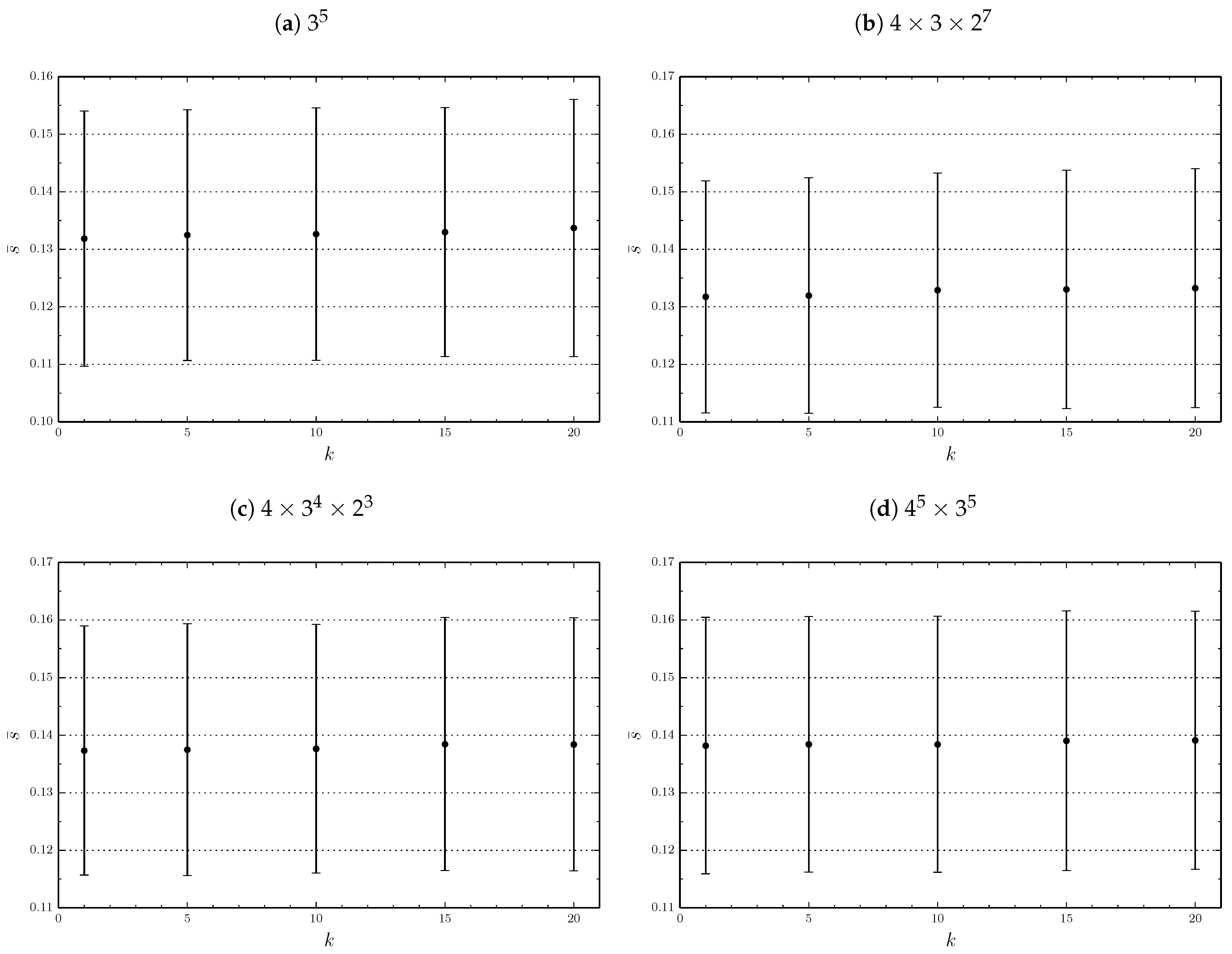
As Figure 2 shows, the normalized prediction error has a very small dependence on k. This is statistically confirmed by the Pearson correlation tests (see Table 3). This result can be explained as follows. For fixed v and r, a smaller k correspond to a larger number of respondents b. Obviously, a larger respondent sample better approximates the real market, and consequently leads to a better accuracy. However, the differences are quite mild: although represents the best choice, it would only lead to a decrease of about 1% in the prediction error compared to . This small gain has to be put in perspective with the price to pay: 10 times more respondents have to be interviewed. For this reason, we do not formulate a strict recommendation for the choice of k. We suggest that the number of profiles presented to each respondent should be only motivated by the load asked to her. For simple products, it can be relatively high (15 to 20) and for complex products relatively low (about 5). Throughout the rest of the present study, we select and keep a middling value for the number of profiles presented to each respondent, namely , which is reasonable from the point of view of the respondent load.
5.4. Number of Profiles in the Basis
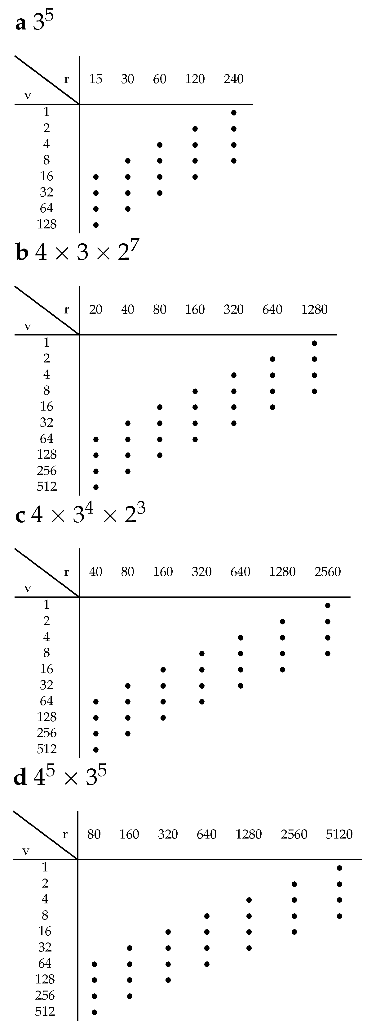
We investigate now the effect of the number v of profiles in the basis on the prediction error. Given that the number of profiles presented to each respondent has been fixed (), we can directly associate the total number of administered profiles with the sample size b by means of the relation . Throughout this subsection, the role of v and r is investigated when the sample size b (and thus ) is held constant. The experimental plans are selected according to Figure 3, where horizontal lines correspond to v, and vertical lines to r. Diagonals from the lower left to the upper right correspond to lines of constant b and contain, within the same factorial design, a constant number of experimental points.
Please note that in the case of the three smallest factorial designs, the largest v among those included in the plan is relatively close to the total number of product design combinations. In contrast, a maximal value is selected in the case of the largest, factorial. The choice of this value, which is by far smaller than the total number of product design combinations, is mainly motivated by computational costs for D-optimality.
As before, 1000 Monte Carlo scenarios are performed, which corresponds to a sample size of 240,000 for the smallest model and 409,960,000 for the biggest one. To separate the effect of b from the one of v and r, we compute
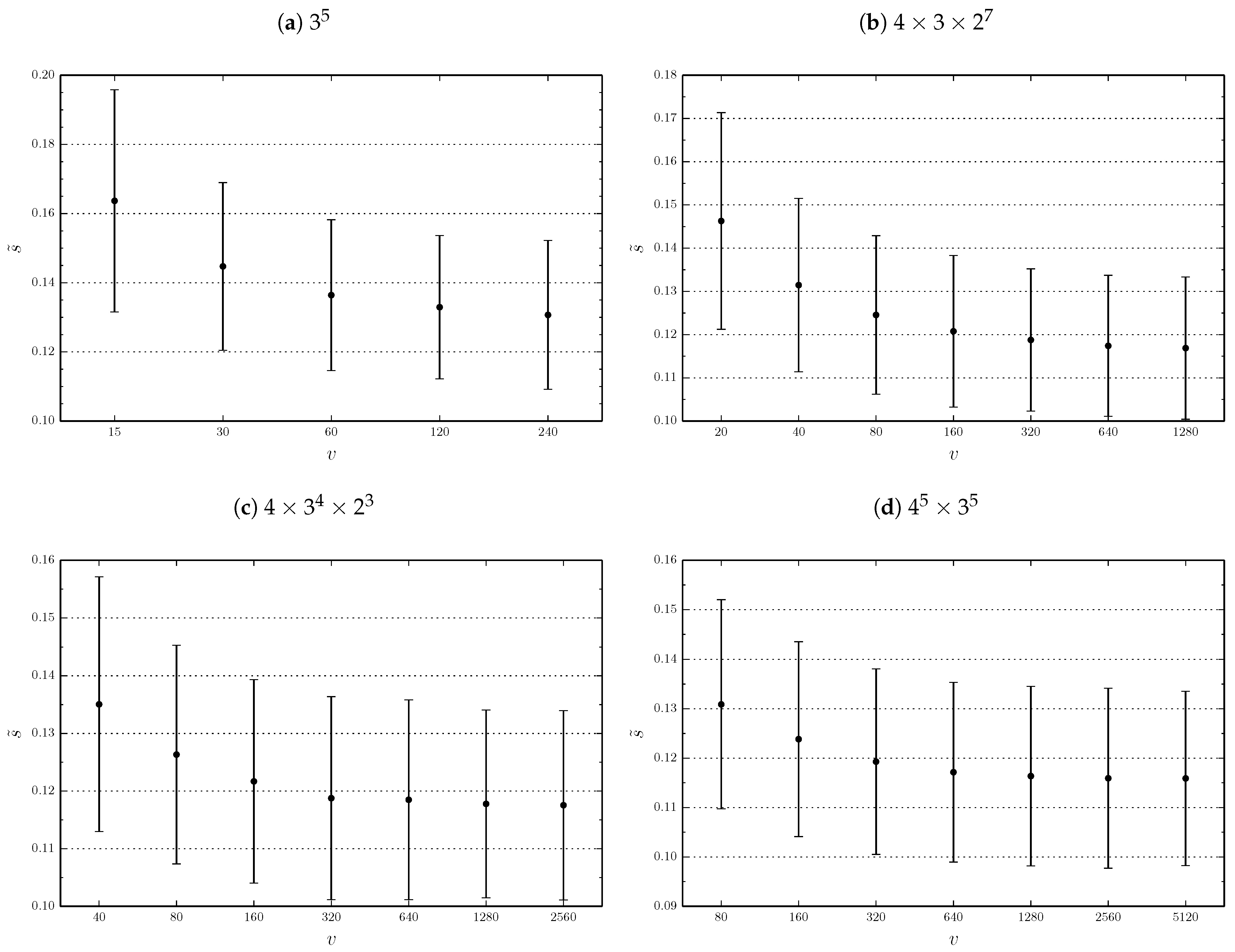
The normalized quantity allows us to superpose the four lines of constant sample size in the numerical analysis. The results are plotted against v in Figure 4. The figure clearly shows that, for fixed b, it is better to increase v rather than r. The gain is stronger in the range of small v (and large r), while it is much weaker, and almost equal to zero, in correspondence of the largest values of v. Because the variation of v and r, given a constant b, has no impact on the questionnaire cost and feasibility, we can formulate a general and simple rule: once b (the number of respondents) and k (the number of profiles presented to each respondent) are selected, take v (the number of profiles in the basis) as large as possible. However, this means that the number of replication is as small as possible. If for logistic reasons, it is preferable to have more replications, it is still possible not to follow strictly this rule. The price to pay is not very high as we distinctly see in in Figure 4 that we quickly attains a plateau.
5.5. Comparison with Standard Conjoint Analysis
In this section, we compare our method against the popular full-profile conjoint analysis with rank orders and with parth-worths estimated by OLS regression. More precisely, we will consider two variants of the experimental design for conjoint analysis, namely: orthogonal and D-optimal designs. Let us recall that conjoint analysis permits us to estimate utility functions for each respondent, which in turn, allows us to compute the estimated market share needed for our numerical experiment. We have to compare two methods where the questionnaire administration is slightly different. To perform this comparison, we will take the same total number of profiles presented to the respondents during the whole survey. Assuming that we have only one competition product, this total number, noted N, is equal to for our method and to for the conjoint model, where denotes the number of respondents and the number of profiles administered to each respondent in the conjoint survey. As an important remark, notice that N does not really represents the total effort made to administer the questionnaire. Indeed, in the conjoint case, the respondent must rank the profiles according to her preference, whereas in our method she has to compare each of them with the competition profile. Consequently, the conjoint model requires more mental operations from the respondent. Despite this, because it is difficult to provide a precise measure of the individual effort by rank-ordering profiles, we prefer to take the quantity N as the comparison criterion. Please note that this choice clearly disadvantages our method.
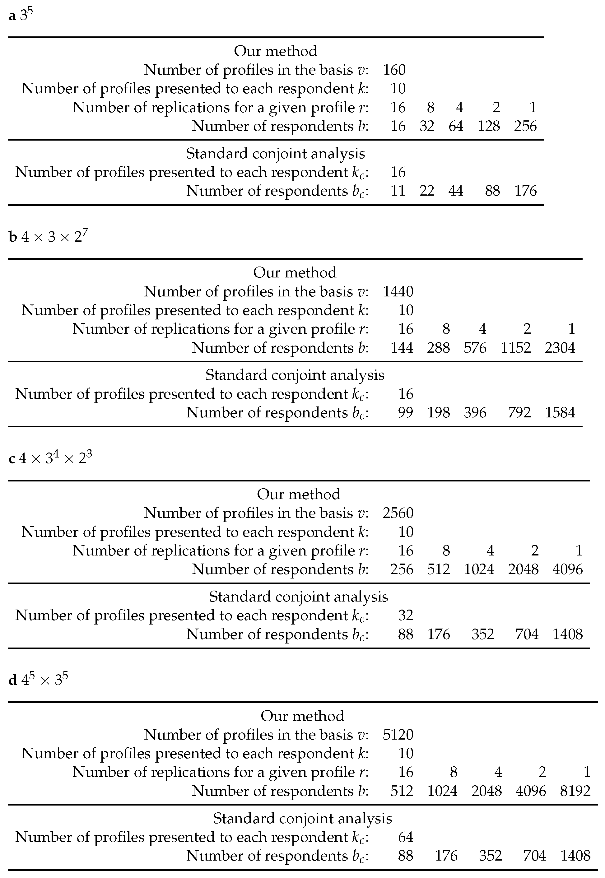
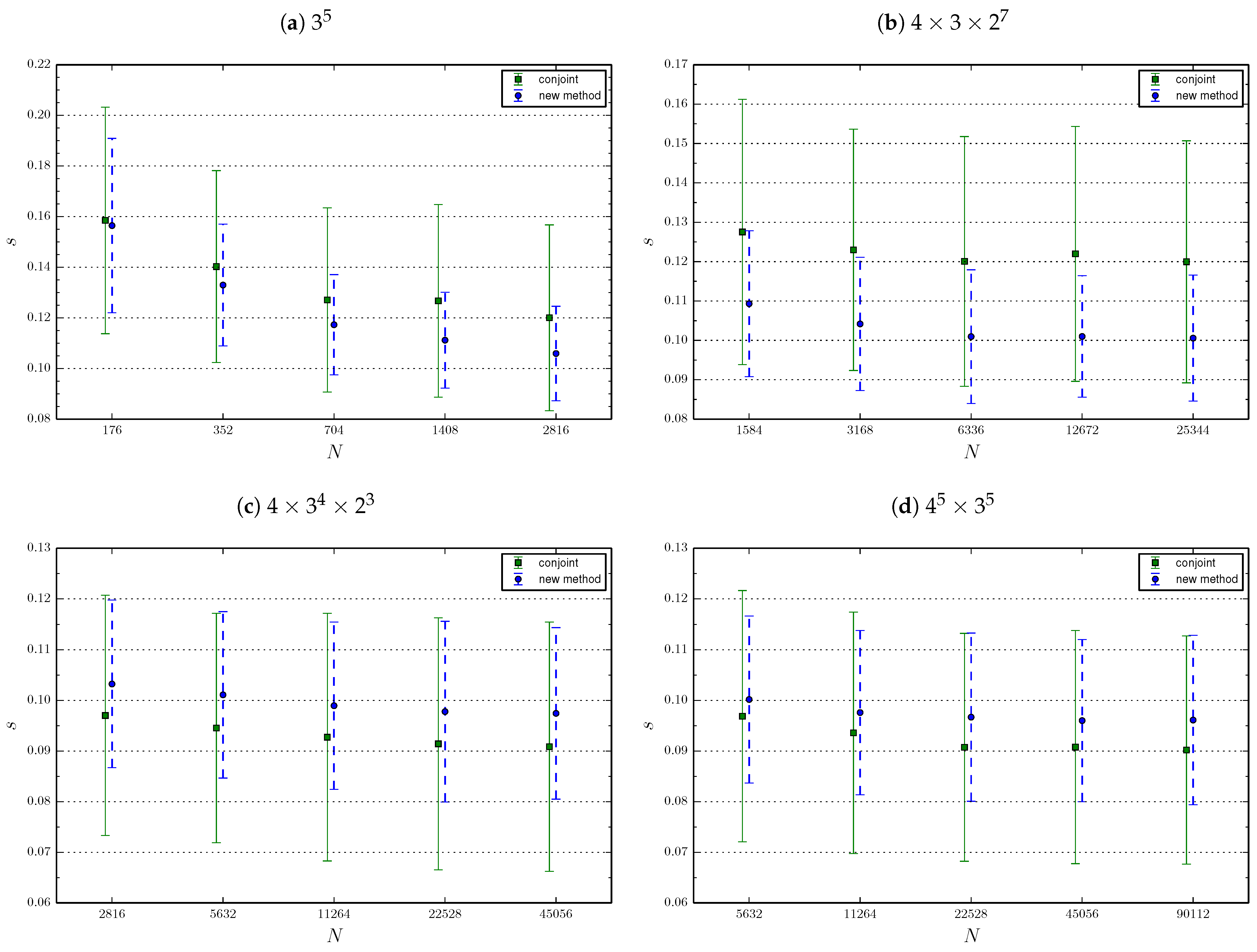
In the first comparison, for conjoint analysis, we use orthogonal plans as calculated by the SPSS software. For this purpose, we use the command ORTHOPLAN (ORTHOPLAN computes a main-effects orthogonal factorial plan) without specifying the minimal number of profiles contained in the design. The number is automatically chosen by the SPSS routine, and is equal to 16 for the and factorials, to 32 for the factorial and to 64 for the factorial. In addition, with fixed, the requirement of comparing both methods at the same value of N puts a constraint on the possible values of v. Under this further condition, and following the rule we found, v is taken to be as large as possible. The experimental plan is given in Figure 5, and the results are shown in Figure 6. Please note that a slight horizontal shift has been added to the figure to improve visualization but, for both methods, the values of N are exactly those indicated by the axes.
We notice that both methods show a similar performance. More precisely, for the two smallest factorial designs, our method behaves a little better than conjoint analysis, while for the two largest factorial designs, conjoint analysis performs a little better. However, in these two latter cases, the conjoint analysis approach is very demanding in terms of respondent effort, so that it is unrealistic to assume that such a questionnaire can be accurately evaluated.
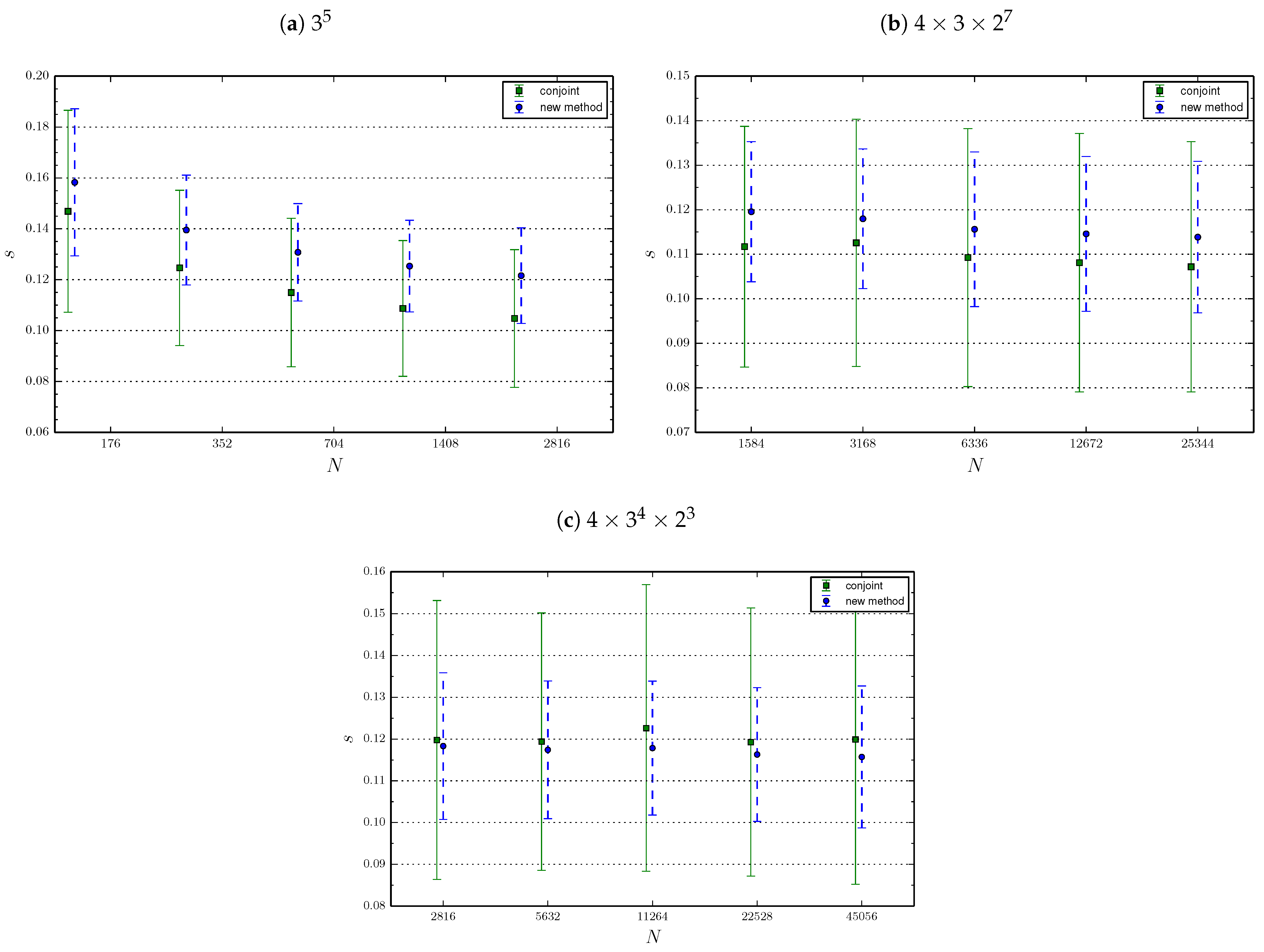
For this reason, a second comparison is made, in which the plans used for the conjoint analysis are D-optimal designs with a fixed number of profiles. This choice has both the advantages of imposing a realistic respondent load and of allowing a comparison at constant . Consequently, we are obliged to omit the largest factorial design, which would require 26 regression parameters to be estimated. The experimental plan for the simulations is identical to the one given by Figure 5 for what concerns the - and the -factorial designs. By contrast, the plan for the -factorial design is modified according to Table 4. The results are shown in Figure 7. As in the previous figure, to improve visualization, a slight horizontal shift has been added to this figure.
Here again, both methods show similar performance. More precisely, conjoint analysis is a little better for the two smallest designs, but performs slightly worse for the largest design. We also see in both figures that our method presents a smaller standard deviation of the prediction error, which means that it leads to more stable predictions. Therefore, we can confidently conclude than the method we propose in the present paper is at least as good as standard conjoint analysis. The price to pay for lowering the amount of information presented to respondents while maintaining performance is to take a larger sample size. In our example, for the small models, we have to take a sample size 1.6 greater than standard conjoint analysis. Please note that we could have chosen to present as many profiles than the standard conjoint analysis to have the same sample size. Finally, for the biggest model, standard conjoint analysis cannot be implemented in reality as the burden on respondents is far too big.
From the numerical experiments, we draw an additional conclusion: Because the slope of the curves gets less and less steep with increasing N for all methods, it is probable that the prediction error will not fall below a certain value even if N is arbitrarily large. For what concerns conjoint analysis, we address this behaviour to the fact that the respondent burden must be rather small (by contrast, if we allowed to equal the total number of possible profiles, the prediction error found in our simulations would approach zero for N large enough). This behaviour also shows a structural limit of the method we propose in this paper. A logistic function of main effects does not actually possess enough degrees of freedom to describe the complicated demand function beyond a certain degree of accuracy. In any case, from the numerical experiments we performed, we observe that the prediction error (which we recall, measures one standard deviation from the true market share of a product profile), lies around 0.1, whatever the method or the factorial design. This value is valid for reasonable sample sizes and should be kept in mind when conducting a real case survey. Including interactions could allow us to lower this structural limit in the case of our method. For conjoint analysis, lowering the limit may be achieved by increasing the number of administered questions to each respondent, but this is hardly an option because respondents would be unable to provide an accurate evaluation of the questionnaire.
As a side remark, we also notice that the accuracy of conjoint analysis improves when using D-optimal designs rather than SPSS-generated orthogonal plans, provided that the number of presented profiles is the same. Indeed, we found that the orthogonal plans that we used are not always balanced and hence not optimal in terms of efficiency (see for instance [55]). D-optimal designs are therefore more suitable for comparing the efficiencies of the different methods.
6. Discussion and Conclusions
The present paper proposes a new approach to estimate the market share for new products. Thanks to a split questionnaire design, our approach permits us to reduce the burden on each respondent as much as desired. Hence, our approach can be used even when the number of attributes and levels is large. However, if one wants to maintain the performance, the price to pay is an increase of the sample size. The software provided as Supplementary Material allows practitioners to implement the method in a user-friendly way. It can be employed to design the split questionnaire and then, once the survey is conducted, to compute the market share estimations.
The method was selected among various alternatives by employing both theoretical arguments and Monte Carlo simulations. As a result, we chose to use a modified Fedorov algorithm to construct a D-optimal basis, and a random block algorithm to administrate subsets of the basis to each respondent. Given the users’ desired questionnaire size, we provide an algorithm that stays close to the wished values and at the same maximizes the size of the D-optimal basis so as to increase efficiency. Indeed, for a given questionnaire size, we found that the method performs better when the same profiles are replicated less and the size of the basis is larger. In contrast, the number of questions administered to each respondent has been shown to play little or no influence onto the overall performance, and for this reason the user is free to specify the value she wishes. Finally, we found that a logistic function of main effects, while being analytically simple, is well-suited for estimating the demand function.
To assess the statistical performance of our new approach, we compared it with standard full-profile conjoint analysis with rank orders and with parth-worths estimated by OLS regression. For this purpose, we conducted further Monte Carlo simulations and can confidently conclude that the method we propose is at least as good as standard conjoint methods. These numerical experiments also show that both methods exhibit a structural limit. The prediction error does not fall below a certain value, which lies around 0.1, even if the sample is taken arbitrarily large. This accuracy is attained for relative small sample sizes: one hundred respondents seem to be sufficient. To our knowledge, even for conjoint analysis, this is the first time that this structural limit is exhibited and quantified.
The method proposed in this paper presents a weakness that is shared with all full-profile approaches. Indeed, a practical size limit may still be imposed by the problem we mentioned in the introduction; i.e., the risk of presenting product descriptions that are too complex for being accurately evaluated by the respondent. However, the choice task demanded to the respondent (that simply consists of stating her own preference between two products) may be regarded as a simulation of what happens in a real market, in which consumers can still be confused by product complexity. Our method presents two further weaknesses that conjoint analysis does not have. First, inferences on a single respondent cannot be done. This disqualifies the method if the main goal is to study market segmentation, but is not an issue otherwise. Second, the competition’s product profiles have to be known prior administrating the survey and, if they change, a new survey must be conducted. This is obviously penalizing but we are currently extending our method to fix this problem by using a multinomial logit approach. Our method is not the only one which tries to reduce the burden on each respondent. For instance adaptive choice-based conjoint [26], hybrid methods [29] or bridging methods [14] do the same. However, contrary to these methods, our method permits a total control of the burden and can therefore be used even when the other methods are not any more implementable.
To conclude, taking all into account, we recommend that our method should be used in the case where the concurrence profiles are not expected to change in the short term, and when the main advantages of our method can be better exploited, i.e., when the number of attributes and levels is large.
Supplementary Materials
The following are available online at https://0-www-mdpi-com.brum.beds.ac.uk/2297-8747/26/1/7/s1, File: PrefShare.zip, PrefShare_tutorial.pdf.
Author Contributions
Conceptualization, methodology, writing—review and editing, S.B. and F.M.; software, numerical experiment, writing—original draft preparation, S.B.; supervision, project administration, funding acquisition, F.M. All authors have read and agreed to the published version of the manuscript.
Funding
This research was funded by the Swiss National Science Foundation grant number 100018_165882.
Conflicts of Interest
The authors declare no conflict of interest. The funders had no role in the design of the study; in the collection, analyses, or interpretation of data; in the writing of the manuscript, or in the decision to publish the results.
References
- Green, P.E.; Rao, V.R. Conjoint Measurement for Quantifying Judgmental Data. J. Mark. Res. 1971, 8, 355–363. [Google Scholar]
- Louviere, J.J. Analyzing Decision Making: Metric Conjoint Analysis; SAGE Publishing: Nelson, BC, Canada, 1988. [Google Scholar]
- Louviere, J.J. Conjoint Analysis Modelling of Stated Preferences: A Review of Theory, Methods, Recent Developments and External Validity. J. Transp. Econ. Policy 1988, 22, 93–119. [Google Scholar]
- Wittink, D.R.; Cattin, P. Commercial Use of Conjoint Analysis: An Update. J. Mark. 1989, 53, 91–96. [Google Scholar] [CrossRef]
- Green, P.E.; Srinivasan, V. Conjoint Analysis in Marketing: New Developments with Implications for Research and Practice. J. Mark. 1990, 54, 3–19. [Google Scholar] [CrossRef]
- Carroll, D.J.; Green, P.E. Psychometric Methods in Marketing Research: Part I, Conjoint Analysis. J. Mark. Res. 1995, 32, 385–391. [Google Scholar]
- Hauser, J.R.; Rao, V.R. Conjoint Analysis, Related Modeling, and Applications. In Marketing Research and Modeling: Progress and Prospects: A Tribute to Paul E. Green; Wind, Y., Green, P.E., Eds.; Kluwer Academic Publishers: New York, NY, USA, 2004; pp. 141–168. [Google Scholar]
- Rao, V.R. Developments in Conjoint Analysis. In Handbook of Marketing Decision Models; Wierenga, B., Ed.; Springer: New York, NY, USA, 2008; pp. 23–55. [Google Scholar]
- Agarwal, J.; Desarbo, W.S.; Malhotra, N.K.; Rao, V.R. An Interdisciplinary Review of Research in Conjoint Analysis: Recent Developments and Directions for Future Research. Cust. Needs Solut. 2015, 2, 19–40. [Google Scholar]
- Cattin, P.; Wittink, D.R. A Monte-Carlo Study of Metric and Nonmetric Estimation Methods for Multiattribute Models; Research Paper 341, Graduate School of Business; Stanford University: Stanford, CA, USA, 1976. [Google Scholar]
- Carmone, F.J.; Green, P.E.; Jain, A.K. Robustness of Conjoint Analysis: Some Monté Carlo Results. J. Mark. Res. 1978, 15, 300–303. [Google Scholar]
- Green, P.E.; Srinivasan, V. Conjoint Analysis in Consumer Research: Issues and Outlook. J. Consum. Res. 1978, 5, 103. [Google Scholar]
- Green, P.E. On the Design of Choice Experiments Involving Multifactor Alternatives. J. Consum. Res. 1974, 1, 61–68. [Google Scholar] [CrossRef]
- Baalbaki, I.B.; Malhotra, N.K. Standardization versus Customization in International Marketing: An Investigation Using Bridging Conjoint Analysis. J. Acad. Mark. Sci. 1995, 23, 182–194. [Google Scholar]
- Green, P.E.; Goldberg, S.M.; Montemayor, M. A Hybrid Utility Estimation Model for Conjoint Analysis. J. Mark. 1981, 45, 33–41. [Google Scholar] [CrossRef]
- Green, P.E.; Krieger, A.M. Individualized hybrid models for conjoint analysis. Manag. Sci. 1996, 42, 850–867. [Google Scholar] [CrossRef]
- Cattin, P.; Gelfand, A.E.; Danes, J. A Simple Bayesian Procedure for Estimation in a Conjoint Model. J. Mark. Res. 1983, 20, 2935. [Google Scholar] [CrossRef]
- Lenk, P.J.; DeSarbo, W.S.; Green, P.E.; Young, M.R. Hierarchical Bayes Conjoint Analysis: Recovery of Partworth Heterogeneity from Reduced Experimental Designs. Mark. Sci. 1996, 15, 173–191. [Google Scholar] [CrossRef]
- Green, P.E. Hybrid Models for Conjoint Analysis: An Expository Review. J. Mark. Res. 1984, 21, 155–169. [Google Scholar] [CrossRef]
- Hofstede, F.T.; Kim, Y.; Wedel, M. Bayesian Prediction in Hybrid Conjoint Analysis. J. Mark. Res. 2002, 39, 253–261. [Google Scholar] [CrossRef]
- Johnson, R.M. Trade-off Analysis of Consumer Values. J. Mark. Res. 1974, 11, 121–127. [Google Scholar]
- Louviere, J.J.; Woodworth, G. Design and Analysis of Simulated Consumer Choice or Allocation Experiments: An Approach Based on Aggregate Data. J. Mark. Res. 1983, 20, 350–367. [Google Scholar]
- Batsell, R.R.; Louviere, J.J. Experimental Analysis of Choice. Mark. Lett. 1991, 2, 199–214. [Google Scholar] [CrossRef]
- Louviere, J.J.; Hensher, D.A.; Swait, J.D. Stated Choice Methods: Analysis and Applications; Cambridge University Press: Cambridge, UK, 2000. [Google Scholar]
- Bradlow, E.T. Current Issues and a “Wish List” for Conjoint Analysis. Appl. Stoch. Models Bus. Ind. 2005, 21, 319–323. [Google Scholar]
- Orme, B.K. Which Conjoint Method Should I Use? Research Paper Series, Sawtooth Software. 2007. Available online: https://sawtoothsoftware.com/resources/technical-papers/which-conjoint-method-should-i-use (accessed on 8 January 2021).
- Toubia, O.; Hauser, J.R.; Simester, D.I. Polyhedral Methods for Adaptive Choice-Based Conjoint Analysis. J. Mark. Res. 2004, 41, 116–131. [Google Scholar] [CrossRef]
- Bradlow, E.T.; Hu, Y.; Ho, T.H. A Learning-Based Model for Imputing Missing Levels in Partial Conjoint Profiles. J. Mark. Res. 2004, 41, 369–381. [Google Scholar] [CrossRef] [Green Version]
- Park, Y.H.; Ding, M.; Rao, V.R. Eliciting Preference for Complex Products: A Web-Based Upgrading Method. J. Mark. Res. 2008, 45, 562–574. [Google Scholar] [CrossRef]
- Scholz, S.W.; Meissner, M.; Decker, R. Measuring Consumer Preferences for Complex Products: A Compositional Approach Based on Paired Comparisons. J. Mark. Res. 2010, 47, 685–698. [Google Scholar] [CrossRef] [Green Version]
- Netzer, O.; Srinivasan, V. Adaptive Self-Explication of Multiattribute Preferences. J. Mark. Res. 2011, 48, 140–156. [Google Scholar] [CrossRef]
- Wittink, D.R.; Cattin, P. Alternative Estimation Methods for Conjoint Analysis: A Monté Carlo Study. J. Mark. Res. 1981, 18, 101–106. [Google Scholar]
- Vriens, M.; Wedel, M.; Wilms, T. Metric Conjoint Segmentation Methods: A Monte Carlo Comparison. J. Mark. Res. 1996, 33, 73–85. [Google Scholar] [CrossRef]
- Chakraborty, G.; Ball, D.; Gaeth, G.J.; Jun, S. The ability of ratings and choice conjoint to predict market shares: A Monte Carlo simulation. J. Bus. Res. 2002, 55, 237–249. [Google Scholar] [CrossRef]
- Andrews, R.L.; Ansari, A.; Currim, I.S. Hierarchical Bayes versus Finite Mixture Conjoint Analysis Models: A Comparison of Fit, Prediction, and Partworth Recovery. J. Mark. Res. 2002, 39, 87–98. [Google Scholar] [CrossRef]
- Andrews, R.L.; Ainslie, A.; Currim, I.S. An Empirical Comparison of Logit Choice Models with Discrete versus Continuous Representations of Heterogeneity. J. Mark. Res. 2002, 39, 479–487. [Google Scholar] [CrossRef] [Green Version]
- Backhaus, K.; Wilken, R.; Hillig, T. Predicting Purchase Decisions with Different Conjoint Analysis Methods: A Monte Carlo Simulation. Int. J. Mark. Res. 2007, 49, 341–364. [Google Scholar] [CrossRef]
- Hein, M.; Kurz, P.; Steiner, W.J. Analyzing the capabilities of the HB logit model for choice-based conjoint analysis: A simulation study. J. Bus. Econ. 2019. [Google Scholar] [CrossRef]
- Cook, R.D.; Nachtsheim, C.J. A Comparison of Algorithms for Constructing Exact D-Optimal Designs. Technometrics 1980, 22, 315–324. [Google Scholar] [CrossRef]
- Nguyen, N.K. Construction of Optimal Block Designs by Computer. Technometrics 1994, 36, 300–307. [Google Scholar]
- Fisher, R.A. The Design of Experiments; Oliver & Boyd: London, UK, 1935. [Google Scholar]
- Yates, F. Complex Experiments. Suppl. J. R. Stat. Soc. 1935, 2, 181–247. [Google Scholar] [CrossRef]
- Yates, F. Incomplete Randomized Blocks. Ann. Eugen. 1936, 7, 121–140. [Google Scholar] [CrossRef]
- Yates, F. The Design and Analysis of Factorial Experiments; Imperial Bureau of Soil Science: Harpenden, UK, 1937. [Google Scholar]
- Barnard, M.M. An Enumeration of the Confounded Arrangements in the 2 × 2 × 2... Factorial Designs. Suppl. J. R. Stat. Soc. 1936, 3, 195–202. [Google Scholar]
- Bose, R.C.; Kishen, K. On the Problem of Confounding in the General Symmetrical Factorial Design. Sankhyā Indian J. Stat. 1940, 5, 21–36. [Google Scholar]
- Plackett, R.L.; Burman, J.P. The Design of Optimum Multifactorial Experiments. Biometrika 1946, 33, 305–325. [Google Scholar]
- Addelman, S. Orthogonal Main-Effect Plans for Asymmetrical Factorial Experiments. Technometrics 1962, 4, 21–46. [Google Scholar]
- Kiefer, J. Optimum Experimental Designs. J. R. Stat. Soc. B Methodol. 1959, 21, 272–319. [Google Scholar] [CrossRef]
- Kiefer, J.; Wolfowitz, J. Optimum Designs in Regression Problems. Ann. Math. Statist. 1959, 30, 271–294. [Google Scholar] [CrossRef]
- Kiefer, J. Optimum Designs in Regression Problems, II. Ann. Math. Stat. 1961, 32, 298–325. [Google Scholar] [CrossRef]
- Kiefer, J.; Wolfowitz, J. The Equivalence of Two Extremum Problems. Can. J. Math. 1960, 12, 363–366. [Google Scholar] [CrossRef]
- Box, G.E.P.; Lucas, H.L. Design of Experiments in Non-Linear Situations. Biometrika 1959, 46, 77–90. [Google Scholar]
- Box, G.E.P.; Hunter, W.G. Sequential Design of Experiments for Nonlinear Models; IBM Data Processing Division: Armonk, NY, USA, 1965; pp. 113–137. [Google Scholar]
- Kuhfeld, W.F.; Tobias, R.D.; Garratt, M. Efficient Experimental Design with Marketing Research Applications. J. Mark. Res. 1994, 31, 545–557. [Google Scholar] [CrossRef] [Green Version]
- Dykstra, O. The Augmentation of Experimental Data to Maximize [X′X]. Technometrics 1971, 13, 682–688. [Google Scholar]
- Fedorov, V.V. Theory of Optimal Experiments; Elsevier: Amsterdam, The Netherlands, 1972. [Google Scholar]
- Mitchell, T.J. An Algorithm for the Construction of “D-Optimal” Experimental Designs. Technometrics 1974, 16, 203–210. [Google Scholar]
- Mitchell, T.J. Computer Construction of “D-Optimal” First-Order Designs. Technometrics 1974, 16, 211–220. [Google Scholar]
- Berger, J.O. Statistical Decision Theory and Bayesian Analysis; Springer: New York, NY, USA, 1985. [Google Scholar]
- Chaloner, K.; Larntz, K. Optimal Bayesian Design Applied to Logistic Regression Experiments. J. Stat. Plan. Inference 1989, 21, 191–208. [Google Scholar] [CrossRef] [Green Version]
- Chernoff, H. Locally Optimal Designs for Estimating Parameters. Ann. Math. Stat. 1953, 24, 586–602. [Google Scholar]
- Pronzato, L.; Walter, É. Robust experiment design via stochastic approximation. Math. Biosci. 1985, 75, 103–120. [Google Scholar]
- Chaloner, K.; Verdinelli, I. Bayesian Experimental Design: A Review. Stat. Sci. 1995, 10, 273–304. [Google Scholar] [CrossRef]
- Burghaus, I.; Dette, H. Optimal designs for nonlinear regression models with respect to non-informative priors. J. Stat. Plan. Inference 2014, 154, 12–25. [Google Scholar] [CrossRef] [Green Version]
- Bornkamp, B. Functional uniform priors for nonlinear modeling. Biometrics 2012, 68, 893–901. [Google Scholar] [PubMed] [Green Version]
- John, J.A. Cyclic Designs; Chapman & Hall: London, UK, 1987. [Google Scholar]
- Steckel, J.H.; DeSarbo, W.S.; Mahajan, V. On the Creation of Acceptable Conjoint Analysis Experimental Designs. Decis. Sci. 1991, 22, 435–442. [Google Scholar]
Figure 1.
The method at a glance.

Figure 2.
Normalized prediction error as a function of the number of profiles presented to each respondents. Dots mark the average value and bars denote one standard deviation.
Figure 2.
Normalized prediction error as a function of the number of profiles presented to each respondents. Dots mark the average value and bars denote one standard deviation.

Figure 3.
Experimental plan to study the interplay between v and r. Diagonals from the lower left to the upper right correspond to subsets of constant .
Figure 3.
Experimental plan to study the interplay between v and r. Diagonals from the lower left to the upper right correspond to subsets of constant .

Figure 4.
Normalized prediction error as a function of the number of profiles in the basis. Dots mark the average value and bars denote one standard deviation.
Figure 4.
Normalized prediction error as a function of the number of profiles in the basis. Dots mark the average value and bars denote one standard deviation.

Figure 5.
Experimental plan to compare our method with standard conjoint analysis. Orthogonal plans generated by SPSS are used for conjoint analysis.
Figure 5.
Experimental plan to compare our method with standard conjoint analysis. Orthogonal plans generated by SPSS are used for conjoint analysis.

Figure 6.
Comparison between our method and conjoint analysis with SPSS-generated plans. The prediction error is plotted as a function of N. Dots mark the average value and bars denote one standard deviation. Round dots correspond to our method, while square dots to standard conjoint analysis.
Figure 6.
Comparison between our method and conjoint analysis with SPSS-generated plans. The prediction error is plotted as a function of N. Dots mark the average value and bars denote one standard deviation. Round dots correspond to our method, while square dots to standard conjoint analysis.

Figure 7.
Comparison between our method and conjoint analysis with D-optimal plans. The prediction error is plotted as a function of N. Dots mark the average value and bars denote one standard deviation. Round dots correspond to our method, while square dots to standard conjoint analysis.
Figure 7.
Comparison between our method and conjoint analysis with D-optimal plans. The prediction error is plotted as a function of N. Dots mark the average value and bars denote one standard deviation. Round dots correspond to our method, while square dots to standard conjoint analysis.


Table 1.
Experimental plan to compare the different methods for splitting the questionnaire.
| Number of profiles in the basis v: | 15 | 30 | 60 | 120 | |
| Number of replications for a given profile r: | 5 | 10 | 25 | 50 | 100 |
| Number of profiles presented to each respondent k: | 5 | 15 |
Table 2.
Experimental plan to investigate the impact of the number of profiles presented to each respondents on the prediction error.
Table 2.
Experimental plan to investigate the impact of the number of profiles presented to each respondents on the prediction error.
| Number of profiles in the basis v: | 20 | 40 | 80 | 160 | |
| Number of replications for a given profile r: | 15 | 30 | 60 | 120 | |
| Number of profiles presented to each respondent k: | 1 | 5 | 10 | 15 | 20 |
Table 3.
Pearson correlation test between the number of profiles presented to each respondent and the normalized prediction error.
Table 3.
Pearson correlation test between the number of profiles presented to each respondent and the normalized prediction error.
| Factorial Model | Correlation Coefficient | p-Value |
|---|---|---|
| 0.033 | < | |
| 0.026 | ||
| 0.018 | ||
| 0.017 |
Table 4.
Experimental plan for the -factorial design for the comparison between our method and standard conjoint analysis with D-optimal plans.
Table 4.
Experimental plan for the -factorial design for the comparison between our method and standard conjoint analysis with D-optimal plans.
| Our Method | |||||
| Number of profiles in the basis v: | 2560 | ||||
| Number of profiles presented to each respondent k: | 10 | ||||
| Number of replications for a given profile r: | 16 | 8 | 4 | 2 | 1 |
| Number of respondents b: | 256 | 512 | 1024 | 2048 | 4096 |
| Standard Conjoint Analysis | |||||
| Number of profiles presented to each respondent : | 16 | ||||
| Number of respondents : | 176 | 352 | 704 | 1408 | 2816 |
Publisher’s Note: MDPI stays neutral with regard to jurisdictional claims in published maps and institutional affiliations. |
© 2021 by the authors. Licensee MDPI, Basel, Switzerland. This article is an open access article distributed under the terms and conditions of the Creative Commons Attribution (CC BY) license (http://creativecommons.org/licenses/by/4.0/).
Share and Cite
MDPI and ACS Style
Balmelli, S.; Moresino, F. Estimating the Market Share for New Products with a Split Questionnaire Survey. Math. Comput. Appl. 2021, 26, 7. https://0-doi-org.brum.beds.ac.uk/10.3390/mca26010007
AMA Style
Balmelli S, Moresino F. Estimating the Market Share for New Products with a Split Questionnaire Survey. Mathematical and Computational Applications. 2021; 26(1):7. https://0-doi-org.brum.beds.ac.uk/10.3390/mca26010007
Chicago/Turabian StyleBalmelli, Simone, and Francesco Moresino. 2021. "Estimating the Market Share for New Products with a Split Questionnaire Survey" Mathematical and Computational Applications 26, no. 1: 7. https://0-doi-org.brum.beds.ac.uk/10.3390/mca26010007