Semi-Supervised Learning Using Hierarchical Mixture Models: Gene Essentiality Case Study

Abstract

Integrating gene-level data is useful for predicting the role of genes in biological processes. This problem has typically focused on supervised classification, which requires large training sets of positive and negative examples. However, training data sets that are too small for supervised approaches can still provide valuable information. We describe a hierarchical mixture model that uses limited positively labeled gene training data for semi-supervised learning. We focus on the problem of predicting essential genes, where a gene is required for the survival of an organism under particular conditions. We applied cross-validation and found that the inclusion of positively labeled samples in a semi-supervised learning framework with the hierarchical mixture model improves the detection of essential genes compared to unsupervised, supervised, and other semi-supervised approaches. There was also improved prediction performance when genes are incorrectly assumed to be non-essential. Our comparisons indicate that the incorporation of even small amounts of existing knowledge improves the accuracy of prediction and decreases variability in predictions. Although we focused on gene essentiality, the hierarchical mixture model and semi-supervised framework is standard for problems focused on prediction of genes or other features, with multiple data types characterizing the feature, and a small set of positive labels.

1. Introduction

Many biomedical investigations now involve the analysis of a large and growing range of genome scale data types, including DNA sequence-derived variables, gene expression measurements, and epigenetic information. Each of these data types can provide valuable information about the complex factors contributing to a biological system, but none by itself can provide a complete picture. The need for integrative modeling approaches to realize the full potential of data growing in diversity as well as volume has been widely recognized over the last several years. Several large consortia, such as ENCODE, have been formed for the purpose of generating and analyzing multiple data sources and have also developed analysis tools for specific research domains [1,2,3,4].

Here we focus on a gene-centric approach, wherein data from genes and their cis- regulatory regions are used to identify particular processes and phenotypes in which that gene plays a role. Although there have been many promising applications for this approach, such as annotating gene function [5], or predicting genes associated with disease pathogenesis (e.g., Reference [6]), we focus on predicting gene essentiality. An essential gene is required for the survival of an organism under a given biological context [7,8]. Because of this, identifying essential genes is important for understanding the basic principles of cellular function. In addition, essential genes can affect how synthetic microorganisms are engineered, and inform the development of effective antibiotics and other drugs [9,10]. Although often focused on model organisms such as bacteria and yeast, several recent studies have also sought to catalog gene essentiality in humans [11].

Essential genes can be determined by a variety of experimental methods, and are reported in several databases [12,13]. Because of the expense and labor involved with the experimental approaches, computational methods have been developed for the purpose of predicting essential genes, and machine learning methods that rely on training a classifier using examples of essential genes have become a common strategy [14,15]. Several features have been used to predict essential genes including both features of the DNA sequence such as GC content, and measured or predicted features of the translated proteins such as hydrophobicity. See Dong et al. [16] for a comprehensive summary of the features most commonly used for predicting essential features. The authors identify five most common classes of features: evolutionary conservation, domain information, network topology, sequence component, and expression level. Another recent review [17] surveys how network topology is also used for predicting essential genes. All potential features may be expected to have some predictive value for essentiality, but many are not particularly strong predictors by themselves. By combining these measures, the hope is to predict essential genes with a much higher degree of sensitivity and specificity than would be possible with any one measure alone.

In many studies, genomic data integration has focused on supervised classification approaches which require high-quality training sets with both positive and negative controls [18,19,20]. When available training data sets are small, unreliable, or incomplete, unsupervised methods are more commonly used [21,22,23,24]. However, even training data whose labels are too incomplete for supervised approaches can provide valuable information beyond unsupervised analysis. In this work, we describe the extension of the unsupervised methods first described in [25] to allow the use of any available positively labeled training data, even if limited, for semi-supervised learning. Alexandridis et al. [26] describe an ad hoc method for semi-supervised mixture modeling with incomplete training data. We build on their work and the more rigorous approach of [27] to develop semi-supervised hierarchical mixture models for any type of training data, specifically designed to deal with the case when only positive examples such as known essential genes are available, often called “positive unlabeled learning” or PUL [28].

Specifically, we describe a mixture model for a single data source, followed by a hierarchical mixture model for multiple data sources (e.g., sequence based, expression). Using cross-validation runs to evaluate a real world genomic scenario where an investigator may only have a small number of known positive labels, we show that the inclusion of positively labeled samples in a semi-supervised learning framework in addition to the hierarchical mixture model improves our ability to detect genes of interest when there is a small training set. Although our case study is on gene essentiality, our framework is general for any gene-centric problem, or other unit such as a metabolite, with multiple data types characterizing the gene (or unit), and a small set of positive labels.

2. Methods

We use a generative mixture model approach to represent classes of genes such as essential vs. nonessential, with a hierarchical structure to represent different types of data and the relationships between them. Mixture models have a long history and a rigorous statistical framework for inference and prediction [29]. Hierarchical mixture models have been applied in other contexts [30] and in a variety of bioinformatic applications [31,32]. In this work, the model can be represented as a graph, where nodes represent random variables, which may be hidden or observed, and the edges represent the conditional dependence structure of the variables. This approach allows for simultaneous modeling of a wide range of data sources (continuous, categorical, etc.), with computationally efficient model fitting and easily interpretable results. To build up to the hierarchical model, we first describe an unsupervised method for single mixture models in Section 2.1, and how that can be adapted to the semi-supervised method for single mixture models in Section 2.3. Then we extend these ideas to hierarchical mixture models for data integration, both unsupervised and semi-supervised in Section 2.4 and Section 2.5, with the latter being our final model.

2.1. Single Mixture Model: Unsupervised Method

A generative mixture model arises when we wish to model the distribution of one random variable X, which depends on the value of another random variable Y, so we say that Y generates X. We assume Y is a univariate categorical random variable that can take on one of K categories (1, …, K), while X, which may be multivariate, can have any distribution. For notational compactness, let $f_y\left(x\right)=f\left(x\right|Y=y)$, and $f\left(x\right)={\sum }_k{p}_k{f}_k\left(x\right)$, with $k=1,\dots ,K$ and ${\sum }_k{p}_k=1$. We also assume we observe X, but not Y—that is, Y is hidden. In our examples, typically $K=2$, for example “non-essential” versus “essential”. The model may also be represented graphically, as shown in Figure 1a. Our challenge is to infer the parameters $\theta$ (e.g., Gaussian mean and variance for each mixture component), which will allow us to calculate expected values for these hidden states. The joint density of X and Y is therefore $f(x,y|\theta )=p_y{f}_y\left(x\right|\theta )$.

From this, for a sample $X=(x_1,\dots ,x_N)$, we use the EM algorithm [33,34] to estimate the parameters and find the posterior probabilities ${\widehat{w}}_{n,y}=P(y_n=y|x_n,\widehat{\theta })$. Specifically, the EM algorithm finds the maximum likelihood estimate $\widehat{\theta }$ by iterative maximization of the “Q-function”, or the conditional expected log-likelihood

$$Q\left(\theta \right|{\theta }^{(i-1)})=E_Y\left[{\sum }_{n}logf(x_n,y_n|\theta )|X,{\theta }^{(i-1)}\right]$$

(1)

where ${\theta }^{(i-1)}$ is the previous iteration’s i estimate for the parameters. For the current model,

$$Q\left(\theta \right|{\theta }^{(i-1)})={\sum }_{n,k}{w}_{n,k}\{log{p}_k+log{f}_k\left(x_n\right|{\theta }^{(i-1)})\}$$

(2)

where

$$w_{n,y}=P(y_n=y|x_n,{\theta }^{(i-1)})=\frac{p_y^{(i-1)}{f}_y\left(x_n\right|{\theta }^{(i-1)})}{{\sum }_k{p}_k^{(i-1)}{f}_k\left(x_n\right|{\theta }^{(i-1)})}.$$

(3)

Generally, $w_{n,1}$ is the posterior probability that $y_n=1$ given the data. In the problems at hand, $w_{n,1}$ is the posterior probability that gene n is essential given the particular data source being used.

Depending on the data type and the distribution, different functional forms for f may be appropriate (e.g., discrete, continuous). In addition within a data type, different alternatives may be available. For example, the Poisson distribution may be compared to the negative binomial, and the Gaussian distribution may be compared to a longer tailed distribution like the Pearson Type VII distribution, which is a general class of distributions and contains the Student’s t distribution. For model selection among forms of f, we use the integrated complete likelihood Bayesian information criterion (ICL-BIC) [35] described in the Supplementary Methods.

2.2. Training Data

For the essential gene problem, there may be a set of known essential genes for a particular organism. In many organisms this set may not be complete. Therefore, it may be useful to use information from the already identified essential genes to predict additional essential genes in an informed manner, which would improve prediction compared to a completely unsupervised approach. Ideally, supervised learning can be used, but in some cases there may not be both positive and negative examples, or the number of known essential genes may be small, therefore we focus on the semi-supervised training scenario. For the essential gene case study, the previously known essential genes are considered to be ‘labeled’ samples in our framework. The authors in [26,36] describe a method for including labeled data in the standard categorical mixture models, which we refer to here as the single mixture model: briefly, at the end of each E-step, update the posterior probabilities for the labeled samples based on their labels. For example, if the nth gene is known to be in category 1 ($y_n=1$) then we would set $w_{n,1}=1$ and $w_{n,k}=0\forall k\ne 1$, regardless of the values of $(w_{n,1},\dots ,w_{n,K})$ calculated previously. The work in [27] presents a more principled approach of incorporating training data into the model as an additional type of observed data, which they apply in a support vector machine (SVM) context. Here we apply their approach in a mixture model context to extend both the single and hierarchical mixture models, with an emphasis on the positive unlabeled learning (PUL) context in which only positive examples are known.

2.3. Single Mixture Model: Semi-Supervised Method

In the presence of partial training data, such as when only a few positive labels are known, we define a new random variable, T, to represent the training labels, in addition to the observed data X and hidden states Y. T is a categorical random variable that can take on the values from $1,\dots ,K^{trn}$, where $K^{trn}=K+1$. If the training label is known for an observation, then $T\le K$. When the training label is unknown for an observation, then $T=K^{trn}$, which is always the case in the unsupervised model. In other words, $P(Y=T|T\le K)=1$ always, while $P(Y=y|T=K^{trn})$ is a free parameter to be estimated. Let ${\overrightarrow{R}}^{trn}$ be the $K^{trn}\times K$ matrix such that $r_{t,y}^{trn}=f\left(y\right|t)=P(Y=y|T=t)$, and observe that the top K rows of ${\overrightarrow{R}}^{trn}$ are fixed at ${\overrightarrow{I}}_K$, the $K\times K$ identity matrix, while the $K^{trn}$th row is free:

$${\overrightarrow{R}}^{trn}=\left(\begin{array}{ccc}1& \cdots & 0\\ ⋮& \ddots & ⋮\\ 0& \cdots & 1\\ r_{K^{trn},1}^{trn}& \cdots & r_{K^{trn},K}^{trn}\end{array}\right)$$

(4)

subject to the constraint ${\sum }_k{r}_{K^{trn},k}^{trn}=1$. In contrast to fully supervised learning methods, this formulation allows us to estimate parameters using information from both labeled and unlabeled samples simultaneously, and also to make use of label information when only positive labels are available.

We incorporate the labels into the model as the sample $\overrightarrow{t}=(t_1,\dots ,t_N)$. For example, in our example application ($K=2$ for “essential” or “non-essential”), we may have some genes known to be essential while others are of unknown binding status. Then for $m,n\in \{1,\dots ,N\}$, $t_m=1$ when we know that the mth gene is essential, while $t_n=3$ when the status of the nth gene is unknown. If we knew the mth gene to be non-essential, we would have $t_m=2$, but our analysis here does not consider the case of labeled negative samples. Conceptually, Y generates both T and X; those samples for which $T\le K$ may be thought of as samples for which Y is observed rather than hidden. We assume the values of T are accurate, that is, there are no unlabeled samples. The model is illustrated graphically in Figure 1b.

However, because of the fixed relationship between Y and $T\le K$, it is more practical to perform most of the calculations on the model as though T generated Y. To obtain ${\widehat{\overrightarrow{R}}}^{trn}$, we need only find the MLE for the $K^{trn}$th row of ${\overrightarrow{R}}^{trn}$, that is, ${\widehat{\overrightarrow{r}}}_{K^{trn}}^{trn}=({\widehat{r}}_{K^{trn},1}^{trn},\dots ,{\widehat{r}}_{K^{trn},K}^{trn})$. The joint density of all variables in the model is

$$f(t,\overrightarrow{x},y|\theta )=p(T=t)p(Y=y|T=t)p(X=x|Y=y,T=t)$$

(5)

or equivalently $f(t,\overrightarrow{x},y|\theta )=p_t^{trn}{r}_{T,t}^{trn}{f}_y\left(\overrightarrow{x}\right|\theta ),$ where $p_t^{trn}=P(T=t)$, and the Q-function is

$$\begin{array}{ccc}\hfill Q\left(\theta \right|{\theta }^{(i-1)})& =& \sum _{n,k^{trn}}{t}_{n,k^{trn}}^{\prime }log{p}_{k^{trn}}^{trn}\hfill \\ & & +\sum _{n,k^{trn},k}{t}_{n,k^{trn}}^{\prime }{w}_{n,k}log{r}_{k^{trn},k}^{trn}\hfill \\ & & +\sum _{n,k}{w}_{n,k}log{f}_k\left({\overrightarrow{x}}_n\right).\hfill \end{array}$$

(6)

Here $t_{n,t}^{\prime }=I(t_n=t)$, and after some simplification, the central calculation for the E-step is

$$w_{n,y}=P(y_n=y|t_n,{\overrightarrow{x}}_n,{\theta }^{(i-1)})=\frac{r_{t_n,y}^{trn(i-1)}{f}_y\left({\overrightarrow{x}}_n\right|{\theta }^{(i-1)})}{{\sum }_k{r}_{t_n,k}^{trn(i-1)}{f}_k\left({\overrightarrow{x}}_n\right|{\theta }^{(i-1)})}.$$

(7)

The modeling of the observed data is the same as in the unsupervised case. By default, labeled samples are given the same weight as unlabeled samples in the parameter estimations. However, if we have a small training sample, we may choose to assign a higher weight $w^{trn}$ to labeled samples. We provide more information on the selection of weights in the Supplementary Methods.

2.4. Hierarchical Mixture Model: Unsupervised Method

The previous model describes the case when there is only a single data type (e.g., one normally distributed variable) or a multivariate distribution of the same type (e.g., multivariate normal). We present a hierarchical mixture model extending the framework above for any number and types of genomic level data.

At the top of the hierarchies shown in Figure 1c is the hidden categorical random variable $Y_0$, which takes on integer values from 1 to $K_0$ for some integer $K_0>1$. In the problem at hand, we assume $K_0=2$ and $Y_0=1$ corresponds to essential genes. Next, let Z denote the number of data sources, and $z\in \{1,\dots ,Z\}$ denote the zth data source. The intermediate hidden categorical random variables $Y_z$ take on integer values from 1 to $K_z$ for some integer $K_z>1$. The distributions of the $Y_z$’s depend—directly or indirectly, depending on the model topology—on the value of $Y_0$. We also define the observed random variables $X_1,\dots ,X_Z$ (each $X_z$ may be multivariate) where the distribution of $X_z$ depends only on the value of $Y_z$. That is, each $X_z$ is generated by $Y_z$. Each $Y_0$ generates $Y=(Y_1,\dots ,Y_Z)$. This model treats all observed variables as equally important to estimating the distribution of $Y_0$. We have explored alternative conditional relationships among the Y’s in [37].

Given N genes, for $n=1,\dots ,N$ the estimated posterior probability that the nth gene is of interest is $P(y_{0,n}=1|{\overrightarrow{x}}_{·,n},\widehat{\theta })$. Here $y_{0,n}$ is the nth hidden status variable, that is, a realization of $Y_0$. Similarly, $y_{z,n}$ is the hidden realization of $Y_z$ for the nth gene, and ${\overrightarrow{x}}_{·,n}=({\overrightarrow{x}}_{1,n},\dots ,{\overrightarrow{x}}_{Z,n})$ is the observed data for the nth gene, with ${\overrightarrow{x}}_{z,n}$ being a realization of $X_z$. Finally, $\widehat{\theta }$ denotes the estimated parameters of the model. See the Supplementary Methods for full details of the estimation procedure. Briefly, the first step in the hierarchical model fitting is to fit a single mixture model to each data source, as described in the previous section, and choose the number of components $K_z$ and marginal distribution which will be used for that data source. These steps follow the EM algorithm described above, and are used for initialization; the individual model fits can be updated in the full algorithm. Then after the marginal distributions are selected, this is used for initialization of the EM algorithm for the full model. The E-step consists of finding the posterior probabilities, given the data and current iteration of $\theta$, for the hidden states $Y_z$ for all data sources z, and for the primary hidden state $Y_0$. The M-step is a straightforward maximum likelihood estimation for the parameters $\theta$, the marginal distribution of $P(Y_0=y_0)$, and conditional relationships among the hidden variables $P(Y_z=y_z|Y_0=y=0)$. More details are provided in the Supplementary Methods.

2.5. Hierarchical Mixture Model: Semi-Supervised Method

We may add T to the hierarchical models in the same way as to the single mixture model, producing the hierarchical model topologies seen in Figure 1d. The main difference between T and the $X_z$’s in this scenario is that there is no intermediate hidden variable corresponding to T, but rather T is generated directly by $Y_0$. In the Supplementary Methods we provide the details on the corresponding EM algorithm. This method constitutes our final semi-supervised hierarchical method and is abbreviated as Semi-HM.

2.6. Essentiality Application

2.6.1. Feature Description

Multiple data sources have been used to predict essential genes within a species including both features of the DNA sequence such as GC content, and measured and predicted features of the proteins translated from the genes, such as hydrophobicity and subcellular localization. All of the features may be expected to be have predictive value for essentiality, but many are not particularly strong predictors. By combining these measures, the hope is to predict essential genes with a much higher degree of sensitivity and specificity than would be possible with any one measure alone. For example, Liu et al. [38] and Guo et al. [39] have shown the high accuracy of using sequence features for predicting bacterial and human essential genes, respectively. To predict essentiality of the genes in S. cerevisiae, our analysis uses features associated with each gene from two sources: (1) fourteen sequence-derived features from [18] and (2) eight additional features from the Ensembl website [40]. Feature definitions are listed in

Table 1. Description of Features. The sequence-derived features were compiled by Seringhaus [18]. Additional data sources were assembled from the Gerstein labs [53]. Dov expression is the normalized difference between absolute mRNA expression levels [52]. The form of the feature (real, integers, binary, etc) is described in the “Type” column, and closed and open brackets indicate closed and open sets, respectively. “Family” describes the distribution the marginal models utilized in the semi-supervised method. Exploratory data analysis was used to identify appropriate marginal distributions for the features. “K” is the univariate optimized number of predicted classes for each variable. * A total of 3 of 22 features (vacuole, in how many of five proks blast, and intron) were removed from the analysis due to low content (less than 5% of non-zero values). ORF: open reading frame.

	Abbreviation	Description	Type	Family	K
Sequence Derived Features	cytoplasm	Predicted subcellular location: cytoplasm	binary	bernoulli	2
	er	Predicted subcellular location: er	binary	bernoulli	2
	mitochondria	Predicted subcellular location: mitochondria	binary	bernoulli	2
	nucleus	Predicted subcellular location: nucleus	binary	bernoulli	2
	vacuole *	Predicted subcellular location: vacuole	binary	bernoulli	2
	other	Predicted subcellular location: other	binary	bernoulli	2
	tm helix	Number of predicted transmembrane helices	integer	neg bin	2
	l aa	Length of putative protein in amino acid	integer	neg bin	3
	nc	Effective number of codons	(real)	normal	2
	gravy	Hydrophobicity	(real)	normal	2
	gc	% GC content	[real]	gamma	2
	close ratio	% codons one-third base pairs from stop codon	[real]	gamma	2
	rare aa ratio	% of rare aa in translated ORF	[real]	gamma	2
	cai	Codon adaptation index	[real]	gamma	2
Additional Features	intxn partners	Number of interaction proteins	integer	neg bin	3
	blast yeast	Number of related genes in yeast BLAST	integer	neg bin	2
	6 yeast blast	Number of related genes in 6 species of yeast	integer	poisson	2
	5 proks blast *	Number of related genes in 5 prokaryotes BLAST	integer	poisson	2
	intron *	Contains an intron in DNA/RNA sequence	binary	bernoulli	2
	chromosome	Chr number	integer	poisson	2
	dovexpr	Dov Expression	(real)	pearson	3
	chr position	Chr position as % of chromosome length	[real]	gamma	2

. A total of 3 of 22 features (vacuole, in how many of five proks blast and intron) were removed from the analysis due to low content (less than 5% of non-zero values), for a final number of 19 features.

2.6.2. Cross-Validation Strategy: Unsupervised

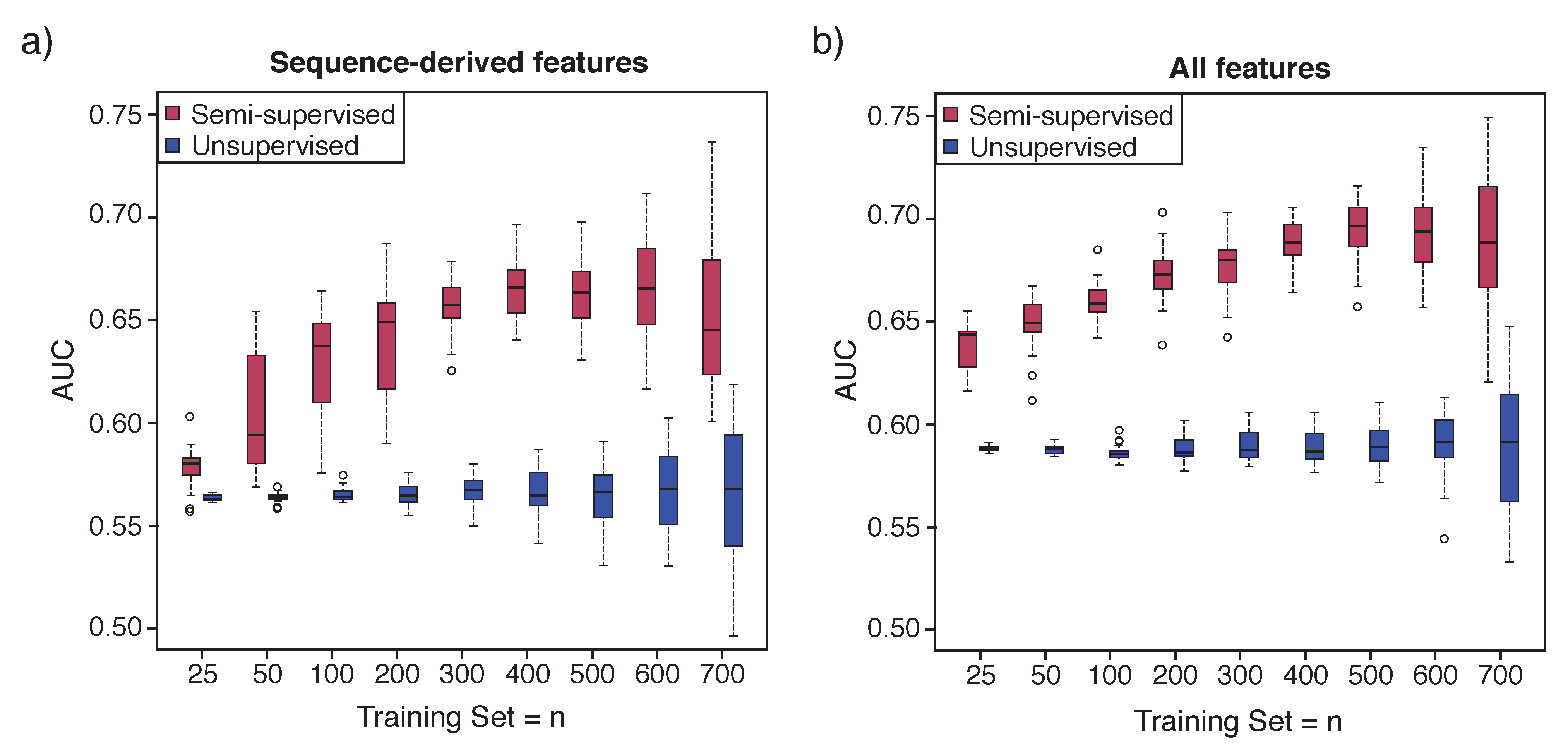
First, for the hierarchical mixture model, the semi-supervised version Figure 1, Model 1d was compared to the unsupervised version Figure 1, Model 1c described in Dvorkin et al. [25]. For the semi-supervised method, we started with the set of 769 essential genes (positive labels) of the total 3500 genes. We performed cross-validation with a range of training set sizes with minimum training set size of 25, chosen to be greater than the number of features to prevent rank deficiency in training sets. For each training set n size, we randomly sampled n essential genes (n = 25 to 700 in increments of 5). Multiple iterations (I = 30) were run to average metrics used to evaluate performance. For the unsupervised method, there is no training set since no information is used to cluster genes. We used $k=2$ to find two clusters, and then the cluster with the highest percentage of essential genes was considered the set of genes predicted as essential, and the other cluster was considered the set of genes predicted as non-essential. We then evaluated prediction performance on the same set of test genes used for the semi-supervised comparison. This procedure was repeated multiple iterations as described above.

2.6.3. Cross-Validation Strategy: Supervised

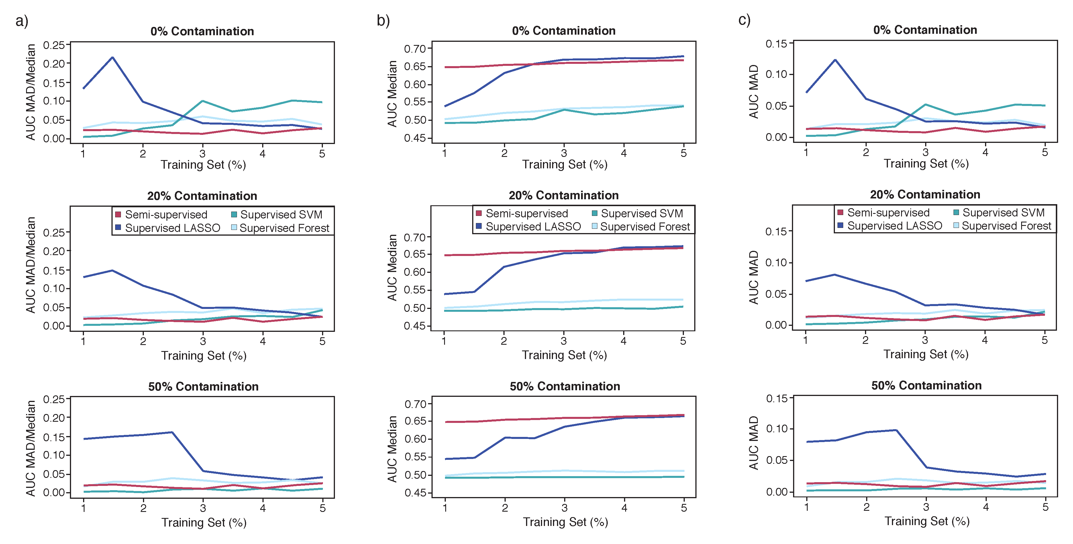
Second, the semi-supervised hierarchical mixture model was compared with other supervised methods. Supervised methods are often used to predict gene essentiality, and require both positive and negative labels. Because of the extensive experimental studies in the yeast S. cerevisiae, we have a comprehensive catalog of essentiality in this model organism. However, in other organisms, we may only have experimental data on a handful of essential genes, which define our known positive labels to be used to predict additional essential genes. In many supervised methods for essentiality, all non-labeled genes are considered to be ‘negatives’ (i.e., non-essential). However, this set may contain additional essential genes, where genes labeled as non-essential may in fact be essential, but have not been confirmed for essentiality yet. That is, these are the yet to be discovered essential genes that are usually considered to be ‘negatives’, when applying supervised methods. We argue this to be the more probable scenario in the essentiality classification because the likelihood of yeast surviving with a knock-out of a truly essential gene regardless of laboratory conditions is nearly zero. Yet, poor nutrient media, uncontrolled temperature regulation during growth phase, or an unknown, unintentional intervention may result in the misclassification from essential to non-essential. Therefore, this results in a situation where essential genes are always labeled positive but a subset of non-essential genes may change status to essential, so they were initially incorrectly labeled as negative. For comparisons with the supervised methods, therefore we introduced this type of contamination, i.e., genes incorrectly labeled as negative, but which are in fact positive (Figure 2). Contamination only affects the negative labels and therefore does not play a role in either unsupervised or semi-supervised methods, but may affect supervised methods.

The cross-validation strategy for the supervised case incorporates an unbalanced strategy to the test set along with a contamination rate, which are described below (Figure 2). For an unbalanced design, test sets utilize the remaining genes not used in the training sets rather than a balanced strategy which matches training and testing set sizes. The unbalanced strategy was chosen because, in practice, an investigator would typically want to test all the remaining genes for essentiality rather than just a subset of genes.

Semi-supervised was compared against three supervised methods (LASSO, SVM, and Random Forests [41,42,43]) at low training set sizes. Performance of these four methods was compared across training set sizes between 1% (n = 35) and 10% (n = 350) from all 3500 genes. Genes randomly chosen for the supervised training sets reflect the same ratio of positive and negative labels as seen in the full data set. Among the 3500 yeast genes, there are 769 essential genes resulting in a 21% ratio. As an example, at 1% training size, 35 randomly chosen genes contained 7 positive labels (21% of 35) and 28 negative labels for supervised methods, while semi-supervised methods were trained on the same training set size, which would be 35 positively labeled genes for this example. We also performed a secondary analysis where the semi-supervised methods had a training set with the same number of positive labeled genes, which would be seven in this example.

In order to mimic contamination, negative labels were reassigned a positive label at rates of 0%, 20%, and 50%. The 20% contamination would correspond to an organism with overall essential gene counts like S. cerevisiae, where the 50% contamination is considered as an extreme example to look at trends in performance due to contamination.

For all results, unique initial seeds were chosen based on the iteration number, training set size, and contamination (for supervised comparison only). Results were summarized over 100 iterations of random sampling. Once the cross-validation data were generated by a seed, the same data were used to compare each method.

2.6.4. Cross-Validation Strategy: Semi-Supervised

As a final comparison, we also evaluated Semi-HM compared to another semi-supervised PUL approach that does not group variables for data integration. We searched the CRAN R package repository for alternative semi-supervised approaches. However, most packages in CRAN are focused on unsupervised or supervised approaches, but there was a recent package AdaSampling [44,45] focused on the PUL problem and utilizes prediction probabilities from a model to iteratively update the unlabeled training data using a variety of different learners. For Semi-HM we applied the same training set selection procedure described above. For AdaSampling, we made adjustments for the training set selection procedure since it requires additional unlabeled data as part of the iterative training process. After setting a percentage of genes positive labels were chosen (e.g., 5% for both Semi-HM and AdaSampling), we randomly selected the same number of negatively labeled genes to be ‘unlabeled’, in addition to a random set of ‘unlabeled’ genes from all other genes using different sizes. For example, for 5% training set size, 175 known positive genes were used for training and the ‘unlabeled’ set consisted of 175 negative genes, and additional genes selected randomly from all other genes (sizes of 50, 100, 300, or 600 were chosen). Performance was assessed on all other genes not included in this process. As classifiers, we tried K Nearest Neighbors (KNN) or logistic regression, which were built into the package. We ran a single classifier, rather than the ensemble approach also available in the package, to be more comparable to Semi-HM.

2.6.5. Algorithms

All cross-validation runs were performed in R version 3.3.3. The semi-supervised and unsupervised analyses detailed in this work utilized functions from the lcmix package. The lcmix package developed and implemented in [25] can be downloaded from http://r-forge.r-project.org/projects/lcmix/ (accessed on 13 May 2021). The other semi-supervised method was performed using the AdaSampling package in R. LASSO was performed using the glmnet command in the glmnet package [46]. Using cv.glmnet, k-fold cross validation optimized the minimum lambda for the LASSO function. SVM analysis used the svm command under the e1071 package [47]. Various runs using different criteria revealed that a radial kernel density and C-classification optimized performance. Random Forest was performed with the randomForest command under the randomForest package [48].

2.6.6. Performance

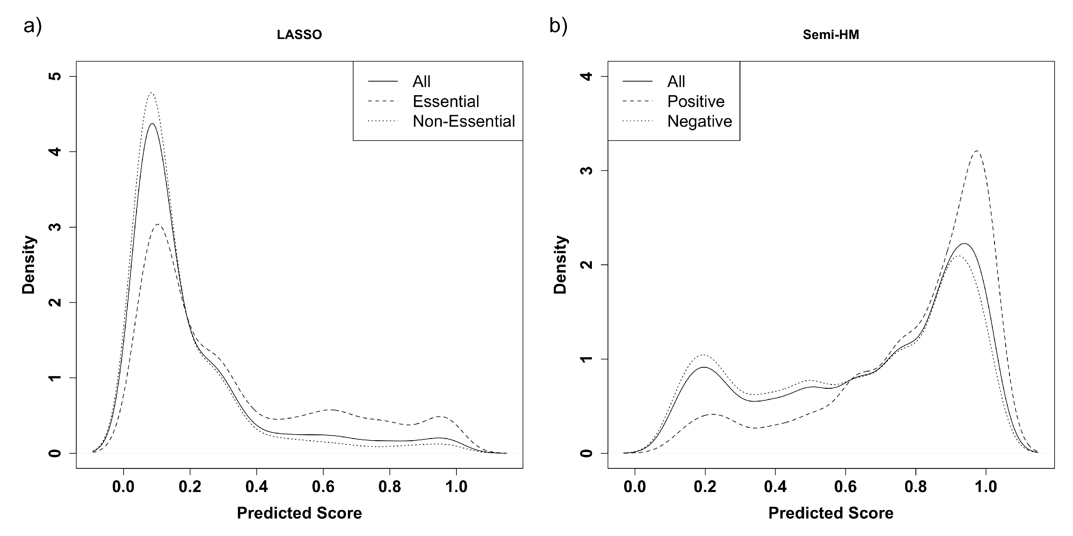
The area under the curve (AUC) was determined using the ROC curve (1-specificity by sensitivity). Then the AUC mean, AUC variance, and a robust coefficient of variation (AUC median absolute deviation/AUC median) of the three supervised methods were contrasted against the semi-supervised method. Because LASSO outperformed the other supervised models in AUC across all training set sizes and contamination rates, a closer evaluation of its performance was compared with the semi-supervised method. In order to fairly compare LASSO performance to the semi-supervised method, the prediction scores were re-scaled to be between 0 and 1. Precision, recall, and f-measure further discriminated the two methods with four rescaled prediction score cutoffs including the median and prediction scores of 0.5, 0.8, and 0.95. The median cutoff is a relative measure based on the data while the other three cutoffs are absolute. The f-measure was calculated from the average precision and recall at each training set size from 1% to 5%.

2.6.7. Gene Enrichment in Saccharomyces cerevisiae

Semi-HM was run using a 10% training size and a posterior probability cutoff of 95% to identify genes as true positives. Enrichment analysis was performed using the Panther Pathway Classification System [49].

2.6.8. Discovery of Essential Genes in Saccharomyces mikatae

The Saccharomyces mikatae genome is not as well annotated as the Saccharomyces cerevisiae genome. Thus, the goal of this application was to show how we can use a more annotated genome to train the model and then use the trained model to make predictions of essentiality on a less annotated genome. Therefore, there were no essentiality labels from the database available, but based on our predictions. Then, we found the orthologs of the predicted genes in S. cerevisiae, where there is annotation, and performed enrichment analysis. Fourteen sequence-derived features were downloaded from the Saccharomyces Genome Database [50] for S. mikatae. One variable, ‘close_stop_ratio’, was removed from analysis due to collinearity with other features. The fitted model from 3500 S. cerevisiae genes was applied to 4551 S. mikatae genes to determine essentiality with a posterior probability cutoff selected visually using the density plot of the posterior probabilities. The cutoff was selected based on the value that separated the bimodal peaks in the density plot. A gene enrichment analysis summarized the predicted essential genes for S. mikatae. To investigate which biological pathways and processes that the S. mikatae open reading frames (ORF) predicted to be essential are involved in, we performed gene enrichment analysis. First, we used the data reported in Seringhaus et al. [18] to identify homologs for each of the ORFs predicted to be essential in our analysis. We used the online Gene Ontology tool [51] to perform enrichment analysis using the Fisher’s test and false discovery (FDR) option.

2.6.9. Availability of Data and Material

The datasets analyzed in this current study are available from [18,52] and the following repositories [40,53].

3. Results

First, we describe each of the features used in the analysis including their data type (e.g., binary, real valued), and report the optimized number of mixtures K and family type for predicting essentiality after fitting the single mixture model (Table 1). Based on the range of univariate estimated AUCs (0.494–0.674), many of the features have low predictive value on their own but in the following comparisons we will explore their combined predictive power. We then used cross-validation to compare our hierarchical mixture model semi-supervised method (Semi-HM) with unsupervised, supervised, and semi-supervised methods.

3.1. Unsupervised Comparison

The complete essentiality data for S. cerevisiae contained n = 769 positive labeled genes. To explore whether our conclusions were sensitive to the choice of features, we first used only 14 sequence-derived features from [18] and then added additional features collected from Ensembl (see Methods). Semi-HM performs better than the unsupervised method for a gain of up to 0.10 AUC regardless of the feature set and training set size (Figure 3), which is not unexpected since the latter does not use any training information. The AUC variance for both methods increased as training size increases when training on all essential genes, which may due to the test set being relatively larger and more constant with the smaller training sets. The additional features generally improve AUC performance and decreases variance for both methods.

3.2. Supervised Comparison

Next, we compared the semi-supervised method with a supervised strategy using all essential genes for the training set and all 19 features. Supervised algorithms require both positive and negative labels. Therefore, we picked a random set of the non-essential genes [54] to be the negative labels (Figure 2), but also included some contamination (some essential positive genes labeled as negatives in the training set) since in practice, the complete set of positive labels will not be known in many situations. Even with the binary outcome, LASSO and Semi-HM outperform the other two supervised methods, SVM and Random Forest (Figure 4). At low training sizes (i.e., 2%, n = 70), Semi-HM method has a higher mean AUC than the three supervised methods. LASSO does not match the stability (lower variance) of Semi-HM until around 5% (n = 175) training set size. However, for larger training set sizes, the AUC variance of Semi-HM increases while variance from LASSO slightly decreases.

We also performed a secondary analysis, where we kept the number of positive labels in the training set for Semi-HM to be the same as the other supervised methods (Supplementary Figure S1). We see similar patterns, where for smaller training set size, the Semi-HM method still has a higher mean AUC than the three supervised methods, but now the training set size where LASSO improves over Semi-HM is smaller than the results in Figure 4. The variance of the AUC for Semi-HM increases because of the smaller training set compared to results in Figure 4, but is still smaller than for LASSO. As contamination increases, all three supervised methods decrease in performance. At 50% contamination, Semi-HM bests all methods across all training set sizes (up to 10%). The AUC robust coefficient of variance (CV; AUC median absolute deviance/AUC median) for Semi-HM is lower than LASSO across all contamination levels and training set sizes up to 5% (Figure 5).

3.3. Semi-HM Versus LASSO Performance

To compare the best performing supervised method, LASSO, for our data to Semi-HM, we took the kernel density of the essentiality prediction scores from each method at 1% training level and rescaled the scores to be between 0 and 1. The solid line in Figure 6 indicates the distribution of scores across genes observed by a user without knowing the true essential or non-essential status, which are indicated in dashed and dotted lines respectively. The two methods show right (Semi-HM) or left skewness (LASSO). However, the more critical issue is whether they show a bimodal pattern. The score from Semi-HM has more of a bimodal shape, where the lower mode is more likely to represent non-essential genes and the higher mode is more likely to represent essential genes. In LASSO, the second mode is much weaker. The uni-modal behavior in LASSO makes it more difficult to find better separation of gene types (e.g., essential versus non-essential). As the training level increases, LASSO kernel densities of prediction scores continue to exhibit unimodal distributions while Semi-HM maintains bi-modal or multi-modal behaviors (data not shown).

Focusing on 0% contamination, the three absolute cutoffs (50%, 80%, and 95%) reveal a higher recall across all training set sizes for Semi-HM and the median cutoff shows Semi-HM outperforming LASSO up to 3% training set size at which they become comparable (Figure 7). Furthermore, up to 3% training set size, Semi-HM outperforms LASSO in precision at the median cutoff. Precision generally increases as the absolute cutoff increases with LASSO besting Semi-HM as training set size increases. Contamination reduces all three performance measures (precision, recall, f-measure) for LASSO across training set sizes from 1% to 5% and all four cutoffs. Irrespective of contamination, f-measure for Semi-HM outperforms LASSO for all training set sizes and cutoffs. Furthermore, the accuracy of LASSO declines with 20% and 50% contamination (Supplementary Figures S2 and S3).

3.4. Semi-Supervised Comparison

One of the main features of Semi-HM is the grouping of genomic variables for an integrated analysis in a hierarchical mixture model framework. To evaluate the benefits of this approach compared to other semi-supervised methods, we used our same essential genes case study and applied the AdaSampling method [44,45], which is another semi-supervised PUL approach that treats all variables equally. Using the same AUC plots, we applied two different versions of AdaSampling, k-nearest neighbor (KNN), or a logistic regression. The KNN version consistently underperformed (data not shown), therefore all results are reported using the logistic regression. In the results, we find similar pattern as with the supervised comparison. Although AdaSampling better performs at larger training set sizes, Semi-HM improves prediction compared to AdaSampling with small training set size, and has smaller variability (Supplementary Figure S4). This pattern was consistent regardless of the number of additional randomly selected genes (50 to 600) were used for training by AdaSampling (data not shown).

3.5. Gene Enrichment in Saccharomyces cerevisiae and Discovery in Saccharomyces mikatae

To demonstrate two applications of the method, first Semi-HM was run using a 10% training set size. For this run, ∼78% of the genes were correctly classified as essential or non-essential. We took a subset of the results to identify if there are differences between the types of genes that are correctly identified as essential (true positives), versus those that are not correctly identified as essential (false negatives). Both groups are enriched in similar types of genes such as those involved in RNA metabolic processes (Supplementary Tables S1 and S2). However, the false negative gene list compared to the true positive gene list was more enriched in pathways related to protein localization, transport, and targeting, in addition to cell cycle and mitosis genes (Supplementary Tables S1 and S2). This suggests further exploration of features that may be discriminating among these gene types.

Second, to demonstrate an application of Semi-HM for discovery, we trained on essential genes in S. cerevisiae, which is well annotated, to predict genes in another genome which is less annotated S. mikatae. Of the 1464 ORFs predicted to be essential using a posterior probability cut-off of 0.70 based on training Semi-HM with all essential genes in S. cerevisiae, 1036 had one homolog in S. cerevisiae. ORFs with multiple or no homologs in S. cerevisiae were excluded from the gene enrichment analysis. Two Gene Ontology pathways were significant with FDR < 0.05: metabolic process (GO:0008152) and catalytic activity (GO:0003824). These results demonstrate that the S. mikatae genes predicted to be essential have homologs in S. cerevisiae that participate in critical processes in the cell [9].

4. Discussion

The focus of the cross-validation runs was to evaluate a real world genomic scenario where an investigator may only have a small number of known positive labels. We compared the semi-supervised hierarchical mixture model to unsupervised, semi-supervised, and supervised methods with multiple data types. Our results indicate that the combination of a hierarchical mixture model and a semi-supervised approach (Semi-HM) improves prediction compared to using one or the other (hierarchical mixture model or semi-supervised). In summary, there were three comparisons. The first comparison (unsupervised method, Figure 3) focuses on the semi-supervised component by comparing a hierarchical mixture model with or without semi-supervised learning. The second comparison (supervised method, Figure 4, Figure 5, Figure 6 and Figure 7) focuses on both components by comparing the hierarchical mixture model and semi-supervised method with leading supervised methods that do not rely on hierarchical mixture models. Although both components are changing, we believe it is important to include a comparison with supervised methods because they are a standard in many applications even with small training sets. Finally the third comparison (semi-supervised, Supplementary Figure S4), focuses on the hierarchical mixture model component by comparing semi-supervised approaches with or without the hierarchical mixture model.

Not unexpectedly because it uses partial information, Semi-HM outperformed the corresponding unsupervised method across a wide range of training set sizes of the essential genes, and data sources. Although Semi-HM outperforms the unsupervised version by utilizing the knowledge of having positive labels, it comes at the cost of some computational time.

For comparisons with the supervised methods, we introduced contamination, by falsely labeling positive genes as negative and not the reverse. We argue this to be the more probable scenario in the essentiality classification because in many prediction methods, all non-known essential genes are treated as negatives (non-essential), but they may in fact be positives (essential) but have not been confirmed yet. Contamination does not play a role in either unsupervised or semi-supervised methods, but may affect supervised methods. Contaminated negative labels causes decreased AUC in the supervised algorithms (Figure 4). However, regardless of contamination rates, the prediction scores for Semi-HM outperformed LASSO in AUC and f-measure at training set sizes below 3%. Furthermore, for these cases, the supervised methods such as LASSO displayed uni-modal distributions of their predicted probabilities. In contrast, the multi-modality of our semi-supervised prediction scores provides a more natural cutoff than the uni-modal distribution displayed by LASSO in Figure 6.

There are alternative semi-supervised methods reviewed in [55]. These methods typically rely on “self-training”, where a supervised classifier is trained on the limited available labeled data, then unlabeled observations are classified. The classifier is then updated based on both the known labels and new predicted labels and this procedure is repeated iteratively until convergence (e.g., Reference [56]). Other methods designed for “positive unlabeled learning” (PUL) identify a set of “reliable” negative observations from the unlabeled data based on features specific to the positive set or other heuristics, and then iteratively repeat the training and prediction process (e.g., References [57,58]). We applied a method designed for PUL called AdaSampling [44,45] and found, as with the previous comparisons, that Semi-HM which relies on hierarchical mixture modeling of predictors shows advantages over other methods when the training set is small.

In general, predicting gene essentiality is challenging as we only observed up to 0.70 for the largest AUC in any of our results. Each of the individual predictors AUC is relatively low, but integrating multiple weak predictors helps performance. Performance for predicting gene essentiality in bacterial species tends to be higher 0.80–0.90 (e.g., References [38,59,60,61]). For yeast, we find that AUC values tend to be lower than for bacterial species. Values range from 0.55 to 0.69 [62], 0.65 to 0.75 [63], 0.77 [64], 0.75 to 0.79 [54], and 0.82 [65]. We have primarily used sequenced based features, with the exception of one expression feature. Some of the cited methods with higher observed AUC use alternative features (e.g., network topology, gene ontology-based features, more gene expression) and larger training set sizes. Our method can be improved by exploring some of these alternative features (see recent review [66]), as was seen in Figure 3 where an expanded feature set provided modest improvement in overall mean and variance of the AUC. Furthermore, exploration of what types of genes are misclassified (Tables S1 and S2) may help suggest the types of features that should be included. However, we specifically focus on the problem of a small positive training set, which occurs in other types of bioinformatics problems. For example, another motivating problem is the prediction of transcription factor target genes based on expression data, DNA binding data and conservation [25]. In that case, there were only 117 known genes regulated in the relevant pathway out of 13,326 Drosophila melanogaster genes, corresponding to 1%, which would be considered a relatively small training set, where Semi-HM shows advantages over other strategies under model misspecification [25].

Finally, we demonstrate an application of Semi-HM where it was trained in a well annotated genome (S. cerevisiae) and then used to predict essential genes in a less annotated genome (S. mikatae). There is no gold standard to evaluate performance so we used the enrichment analysis to explore the results, which indicated genes relevant to essentiality. However, most of the genes predicted to be essential in S. mikatae did not have homologs that were essential genes in S. cerevisiae, which may be explained by a variety of factors including imperfect homology determination. Without a gold standard we cannot benchmark performance but include this analysis as a demonstration, which may be improved within the Semi-HM framework by using additional variables as discussed above (only sequence-derived were used for this demonstration), by using ensemble learning as in [45], and by incorporating imbalanced learning principles [67] since there are fewer essential genes compared to non-essential genes.

5. Conclusions

In summary, using the gene essentiality problem as a case study, a hierarchical mixture modeling approach for semi-supervised learning performs well when there is only a small training set of positive labels. Fully supervised classifiers, and those derived from them such as the “self-training” semi-supervised iterative classifiers, are highly sensitive to even a small amount of error in the training set (e.g., positive genes being mislabeled as negative). The hierarchical mixture model approach may be able to handle such data and extract the useful information from correctly labeled training data while avoiding the detrimental effects of mislabeled data. Furthermore, the hierarchical mixture model also provides a natural framework to integrate any number and type of genomic level data making it applicable to a variety of bioinformatics problems. The R code for the Semi-HM method is available at https://r-forge.r-project.org/projects/lcmix/ (accessed on 13 May 2021).

References

1. The ENCODE Project Consortium. The ENCODE (ENCyclopedia Of DNA Elements) Project. Science 2004, 306, 636–640. [Google Scholar] [CrossRef] [PubMed] [Green Version]
2. The ENCODE Project Consortium. An integrated encyclopedia of DNA elements in the human genome. Nature 2012, 489, 57–74. [Google Scholar] [CrossRef]
3. Celniker, S.; Dillon, L.; Gerstein, M.; Gunsalus, K.; Henikoff, S.; Karpen, G.H.; Kellis, M.; Lai, E.C.; Lieb, J.D.; MacAlpine, D.M.; et al. Unlocking the secrets of the genome. Nature 2009, 459, 927–930. [Google Scholar] [CrossRef] [Green Version]
4. National Cancer Institute. The Cancer Genome Atlas. 2013. Available online: http://cancergenome.nih.gov/ (accessed on 26 May 2013).
5. Troyanskaya, O.G.; Dolinski, K.; Owen, A.B.; Altman, R.B.; Botstein, D. A Bayesian framework for combining heterogeneous data sources for gene function prediction (in Saccharomyces cerevisiae). Proc. Natl. Acad. Sci. USA 2003, 100, 8348–8353. [Google Scholar] [CrossRef] [PubMed] [Green Version]
6. Ward, L.; Kellis, M. Interpreting noncoding genetic variation in complex traits and human disease. Nat. Biotechnol. 2012, 30, 1095–1106. [Google Scholar] [CrossRef] [PubMed] [Green Version]
7. Rancati, G.; Moffat, J.; Typas, A.; Pavelka, N. Emerging and evolving concepts in gene essentiality. Nat. Rev. Genet. 2018, 19, 34–49. [Google Scholar] [CrossRef] [PubMed]
8. Bartha, I.; di Iulio, J.; Venter, J.; Telenti, A. Human gene essentiality. Nat. Rev. Genet. 2018, 19, 51–62. [Google Scholar] [CrossRef]
9. Zhang, Z.; Ren, Q. Why are essential genes essential?—The essentiality of Saccharomyces genes. Microb. Cell 2015, 2, 280–287. [Google Scholar] [CrossRef] [PubMed] [Green Version]
10. Juhas, M.; Eberl, L.; Glass, J.I. Essence of life: Essential genes of minimal genomes. Trends Cell Biol. 2011, 21, 562–568. [Google Scholar] [CrossRef] [PubMed]
11. Wang, T.; Birsoy, K.; Hughes, N.W.; Krupczak, K.M.; Post, Y.; Wei, J.J.; Sabatini, D.M. Identification and characterization of essential genes in the human genome. Science 2015, 350, 1096–1101. [Google Scholar] [CrossRef] [PubMed] [Green Version]
12. Luo, H.; Lin, Y.; Liu, T.; Lai, F.L.; Zhang, C.T.; Gao, F.; Zhang, R. DEG 15, an update of the Database of Essential Genes that includes built-in analysis tools. Nucleic Acids Res. 2020, 49, D677–D686. [Google Scholar] [CrossRef] [PubMed]
13. Gurumayum, S.; Jiang, P.; Hao, X.; Campos, T.; Young, N.; Korhonen, P.; Gasser, R.; Bork, P.; Zhao, X.M.; He, L.J.; et al. OGEE v3: Online GEne Essentiality database with increased coverage of organisms and human cell lines. Nucleic Acids Res. 2020, 49, D998–D1003. [Google Scholar] [CrossRef] [PubMed]
14. Mobegi, F.M.; Zomer, A.; de Jonge, M.I.; van Hijum, S.A.F.T. Advances and perspectives in computational prediction of microbial gene essentiality. Brief. Funct. Genom. 2017, 16, 70–79. [Google Scholar] [CrossRef]
15. Zhang, X.; Acencio, M.L.; Lemke, N. Predicting Essential Genes and Proteins Based on Machine Learning and Network Topological Features: A Comprehensive Review. Front. Physiol. 2016, 7, 75. [Google Scholar]
16. Dong, C.; Jin, Y.T.; Hua, H.L.; Wen, Q.F.; Luo, S.; Zheng, W.X.; Guo, F.B. Comprehensive review of the identification of essential genes using computational methods: Focusing on feature implementation and assessment. Brief. Bioinform. 2018. [Google Scholar] [CrossRef] [PubMed]
17. Li, X.; Li, W.; Zeng, M.; Zheng, R.; Li, M. Network-based methods for predicting essential genes or proteins: A survey. Brief. Bioinform. 2019. [Google Scholar] [CrossRef]
18. Seringhaus, M.; Paccanaro, A.; Borneman, A.; Snyder, M.; Gerstein, M. Predicting essential genes in fungal genomes. Genom. Res. 2006, 16, 1126–1135. [Google Scholar] [CrossRef] [PubMed] [Green Version]
19. Ortiz-Barahona, A.; Villar, D.; Pescador, N.; Amigo, J.; del Peso, L. Genome-wide identification of hypoxia-inducible factor binding sites and target genes by a probabilistic model integrating transcription-profiling data and in silico binding site prediction. Nucleic Acids Res. 2010, 38, 2332–2345. [Google Scholar] [CrossRef]
20. Tyekucheva, S.; Marchionni, L.; Karchin, R.; Parmigiani, G. Integrating diverse genomic data using gene sets. Genom. Biol. 2011, 12, R105. [Google Scholar] [CrossRef] [Green Version]
21. Lemmens, K.; Dhollander, T.; De Bie, T.; Monsieurs, P.; Engelen, K.; Smets, B.; Winderickx, J.; de Moor, B.; Marchal, K. Inferring transcriptional modules from ChIP-chip, motif and microarray data. Genom. Biol. 2006, 7, R37. [Google Scholar] [CrossRef] [Green Version]
22. Xie, Y.; Pan, W.; Jeong, K.; Xiao, G.; Khodursky, A. A Bayesian approach to joint modeling of protein-DNA binding, gene expression and sequence data. Stat. Med. 2010, 29, 489–503. [Google Scholar] [CrossRef] [PubMed] [Green Version]
23. Qin, J.; Li, M.; Wang, P.; Zhang, M.; Wang, J. ChIP-Array: Combinatory analysis of ChIP-seq/chip and microarray gene expression data to discover direct/indirect targets of a transcription factor. Nucleic Acids Res. 2011, 39, W430–W436. [Google Scholar] [CrossRef]
24. Hoffman, M.; Buske, O.; Wang, J.; Weng, Z.; Bilmes, J.; Noble, W. Unsupervised pattern discovery in human chromatin structure through genomic segmentation. Nat. Methods 2012, 9, 473–476. [Google Scholar] [CrossRef] [Green Version]
25. Dvorkin, D.; Biehs, B.; Kechris, K. A graphical model method for integrating multiple sources of genome-scale data. Stat. Appl. Genet. Mol. Biol. 2013, 12, 469–487. [Google Scholar] [CrossRef] [Green Version]
26. Alexandridis, R.; Lin, S.; Irwin, M. Class discovery and classification of tumor samples using mixture modeling of gene expression data—A unified approach. Bioinformatics 2004, 20, 2545–2552. [Google Scholar] [CrossRef]
27. Elkan, C.; Noto, K. Learning classifiers from only positive and unlabeled data. In Proceedings of the 14th International Conference on Knowledge Discovery and Data Mining, Las Vegas, NV, USA, 24–27 August 2008; pp. 213–220. [Google Scholar]
28. He, J.; Zhang, Y.; Li, X.; Wang, Y. Naive Bayes classifier for positive unlabeled learning with uncertainty. In Proceedings of the Tenth SIAM International Conference on Data Mining, Columbus, OH, USA, 29 April–1 May 2010; pp. 361–372. [Google Scholar]
29. McLachlan, G.J.; Peel, D. Finite Mixture Models; Wiley: Chichester, UK, 2000; p. xxii. [Google Scholar]
30. Vermunt, J.; Magidson, J. Hierarchical mixture models for nested data structures. In Classification–the Ubiquitous Challenge: Proceedings of the 28th Annual Conference of the Gesellschaft für Klassifikation eV, University of Dortmund, 9–11 March 2004; Springer: Berlin/Heidelberg, Germany, 2005; Volume 28, p. 240. [Google Scholar]
31. Jörnsten, R.; Keleş, S. Mixture models with multiple levels, with application to the analysis of multifactor gene expression data. Biostatistics 2008, 9, 540–554. [Google Scholar] [CrossRef]
32. Li, Q.; MacCoss, M.; Stephens, M. A nested mixture model for protein identification using mass spectrometry. Ann. Appl. Stat. 2010, 4, 962–987. [Google Scholar] [CrossRef] [Green Version]
33. Dempster, A.; Laird, N.; Rubin, D. Maximum likelihood from incomplete data via the EM algorithm. J. R. Stat. Soc. B Methodol. 1977, 39, 1–38. [Google Scholar]
34. McLachlan, G.; Krishnan, T. The EM Algorithm and Extensions, 2nd ed.; Wiley: Hoboken, NJ, USA, 2008. [Google Scholar]
35. Biernacki, C.; Celeux, G.; Govaert, G. Assessing a mixture model for clustering with the integrated completed likelihood. IEEE Trans. Pattern Anal. Mach. Intell. 2000, 22, 719–725. [Google Scholar] [CrossRef]
36. Ward, G.; Hastie, T.; Barry, S.; Elith, J.; Leathwick, J.R. Presence-Only Data and the EM Algorithm. Biometrics 2009, 65, 554–563. [Google Scholar] [CrossRef] [PubMed] [Green Version]
37. Dvorkin, D. Graphical Model Methods for Integrating Diverse Sources of Genome-Scale Data. Ph.D. Thesis, University of Colorado, Boulder, CO, USA, 2013. [Google Scholar]
38. Liu, X.; Wang, B.J.; Xu, L.; Tang, H.L.; Xu, G.Q. Selection of key sequence-based features for prediction of essential genes in 31 diverse bacterial species. PLoS ONE 2017, 12, e0174638. [Google Scholar] [CrossRef] [PubMed] [Green Version]
39. Guo, F.B.; Dong, C.; Hua, H.L.; Liu, S.; Luo, H.; Zhang, H.W.; Jin, Y.T.; Zhang, K.Y. Accurate prediction of human essential genes using only nucleotide composition and association information. Bioinformatics 2017, 33, 1758–1764. [Google Scholar] [CrossRef] [Green Version]
40. Zerbino, D.R.; Achuthan, P.; Akanni, W.; Amode, M.R.; Barrell, D.; Bhai, J.; Billis, K.; Cummins, C.; Gall, A.; Girón, C.G.; et al. Ensembl 2018. Nucleic Acids Res. 2018, 46, D754–D761. [Google Scholar] [CrossRef] [PubMed]
41. Tibshirani, R. Regression Shrinkage and Selection via the Lasso. J. R. Stat. Soc. B Methodol. 1996, 58, 267–288. [Google Scholar] [CrossRef]
42. Cortes, C.; Vapnik, V. Support-Vector Networks. Mach. Learn. 1995, 20, 273–297. [Google Scholar] [CrossRef]
43. Breiman, L. Random Forests. Mach. Learn. 2001, 45, 5–32. [Google Scholar] [CrossRef] [Green Version]
44. Yang, P.; Liu, W.; Yang, J. Positive unlabeled learning via wrapper-based adaptive sampling. In Proceedings of the Twenty-Sixth International Joint Conference on Artificial Intelligence (IJCAI-17), Melbourne, Australia, 19–25 August 2017; pp. 3273–3279. [Google Scholar] [CrossRef] [Green Version]
45. Yang, P.; Ormerod, J.T.; Liu, W.; Ma, C.; Zomaya, A.Y.; Yang, J.Y.H. AdaSampling for Positive-Unlabeled and Label Noise Learning With Bioinformatics Applications. IEEE Trans. Cybern. 2019, 49, 1932–1943. [Google Scholar] [CrossRef]
46. Friedman, J.; Hastie, T.; Tibshirani, R. Regularization Paths for Generalized Linear Models via Coordinate Descent. J. Stat. Softw. 2010, 33, 1–22. [Google Scholar] [CrossRef] [Green Version]
47. Meyer, D.; Dimitriadou, E.; Hornik, K.; Weingessel, A.; Leisch, F. e1071: Misc Functions of the Department of Statistics, Probability Theory Group (Formerly: E1071), TU Wien. R package version 1.6-8. Available online: https://rdrr.io/rforge/e1071/ (accessed on 13 May 2021).
48. Liaw, A.; Wiener, M. Classification and Regression by randomForest. R News 2002, 2, 18–22. [Google Scholar]
49. Mi, H.; Huang, X.; Muruganujan, A.; Tang, H.; Mills, C.; Kang, D.; Thomas, P.D. PANTHER version 11: Expanded annotation data from Gene Ontology and Reactome pathways, and data analysis tool enhancements. Nucleic Acids Res. 2017, 45, D183–D189. [Google Scholar] [CrossRef] [Green Version]
50. Cherry, J.M.; Hong, E.L.; Amundsen, C.; Balakrishnan, R.; Binkley, G.; Chan, E.T.; Christie, K.R.; Costanzo, M.C.; Dwight, S.S.; Engel, S.R.; et al. Saccharomyces Genome Database: The genomics resource of budding yeast. Nucleic Acids Res. 2011, 40, D700–D705. [Google Scholar] [CrossRef] [Green Version]
51. The Gene Ontology Consortium. The Gene Ontology Resource: 20 years and still GOing strong. Nucleic Acids Res. 2018, 47, D330–D338. [Google Scholar]
52. Jansen, R.; Greenbaum, D.; Gerstein, M. Relating Whole-Genome Expression Data with Protein-Protein Interactions. Genom. Res. 2002, 12, 37–46. [Google Scholar] [CrossRef] [Green Version]
53. Gerstein Lab. Available online: http://www.gersteinlab.org/proj/predess/ (accessed on 13 May 2021).
54. Cheng, J.; Wu, W.; Zhang, Y.; Li, X.; Jiang, X.; Wei, G.; Tao, S. A new computational strategy for predicting essential genes. BMC Genom. 2013, 14, 910. [Google Scholar] [CrossRef] [PubMed] [Green Version]
55. Zhu, X.; Goldberg, A. Introduction to Semi-Supervised Learning; Morgan & Claypool: Williston, VT, USA, 2009; Volume 3. [Google Scholar]
56. Tanha, J.; van Someren, M.; Afsarmanesh, H. Semi-supervised self-training for decision tree classifiers. Int. J. Mach. Learn. Cybern. 2017, 8, 355–370. [Google Scholar] [CrossRef] [Green Version]
57. Yu, H.; Han, J.; Chang, K.C.C. PEBL: Positive Example Based Learning for Web Page Classification Using SVM. In Proceedings of the Eighth ACM SIGKDD International Conference on Knowledge Discovery and Data Mining, (KDD ’02), Edmonton, AB, Canada, 23–26 July 2020; ACM: New York, NY, USA, 2002; pp. 239–248. [Google Scholar]
58. Liu, B.; Lee, W.S.; Yu, P.S.; Li, X. Partially Supervised Classification of Text Documents. In Proceedings of the Nineteenth International Conference on Machine Learning (ICML-2002), Sydney, Australia, 8–12 July 2002; Morgan Kaufmann Publishers Inc.: San Francisco, CA, USA, 2002; pp. 387–394. [Google Scholar]
59. Wei, W.; Ning, L.W.; Ye, Y.N.; Guo, F.B. Geptop: A Gene Essentiality Prediction Tool for Sequenced Bacterial Genomes Based on Orthology and Phylogeny. PLoS ONE 2013, 8, e72343. [Google Scholar] [CrossRef] [PubMed]
60. Nigatu, D.; Sobetzko, P.; Yousef, M.; Henkel, W. Sequence-based information-theoretic features for gene essentiality prediction. BMC Bioinform. 2017, 18, 473. [Google Scholar] [CrossRef] [PubMed] [Green Version]
61. Li, Y.; Lv, Y.; Li, X.; Xiao, W.; Li, C. Sequence comparison and essential gene identification with new inter-nucleotide distance sequences. J. Theor. Biol. 2017, 418, 84–93. [Google Scholar] [CrossRef]
62. Fan, Y.; Tang, X.; Hu, X.; Wu, W.; Ping, Q. Prediction of essential proteins based on subcellular localization and gene expression correlation. BMC Bioinform. 2017, 18, 470. [Google Scholar] [CrossRef] [PubMed] [Green Version]
63. Cheng, J.; Xu, Z.; Wu, W.; Zhao, L.; Li, X.; Liu, Y.; Tao, S. Training Set Selection for the Prediction of Essential Genes. PLoS ONE 2014, 9, e86805. [Google Scholar] [CrossRef] [Green Version]
64. Zhong, J.; Wang, J.; Peng, W.; Zhang, Z.; Pan, Y. Prediction of essential proteins based on gene expression programming. BMC Genom. 2013, 14, S7. [Google Scholar] [CrossRef] [PubMed] [Green Version]
65. Saha, S.; Heber, S. In silico prediction of yeast deletion phenotypes. Genet. Mol. Res. 2006, 5, 224–232. [Google Scholar]
66. Aromolaran, O.; Aromolaran, D.; Isewon, I.; Oyelade, J. Machine learning approach to gene essentiality prediction: A review. Brief. Bioinform. 2021. [Google Scholar] [CrossRef]
67. Blagus, R.; Lusa, L. SMOTE for high-dimensional class-imbalanced data. BMC Bioinform. 2013, 14, 106. [Google Scholar] [CrossRef] [Green Version]
Figure 1. Model Representations. Graphical representation of models for (a) single mixture model, (b) single mixture model with training labels, (c) hierarchical mixture model, and (d) hierarchical mixture model with training labels.
Mca 26 00040 g001
Figure 2. Diagram of training sets for supervised methods, including contamination. The Simulation and True Labels rows describe the label assignment for the cross-validation analysis, and the true labels for gene essentiality, respectively. In the top row, n e s s is the total number of essential genes (769 for our example) and n n o n is the total number of non-essential genes. Of the essential genes, we select a training set percentage p i for training the algorithms. Additional cross-validation trials were performed where a number of contaminated genes n c o n where included in the negative training set (i.e., they are mis-labeled essential genes, see Methods). The shaded area indicates the contamination of training set essential genes where assigned and true labels differ. When n c o n is set to 0, there is no contamination.
Mca 26 00040 g002
Figure 3. Area Under the Curve (AUC) Comparison of Semi-HM versus Supervised Approach. Boxplots are displayed for various training set sizes from the 769 essential genes using either (a) sequence derived predictors only or (b) all features as predictors described in Table 1. Semi-supervised and unsupervised hierarchical mixture model methods are shown in red and blue, respectively.
Mca 26 00040 g003
Figure 4. AUC comparison between Semi-HM and Supervised methods. The final set of 19 features from Table 1 were used as predictors. A total of 100 iterations were executed at training sets percentages (1, 1.5, 2, …, 10) for all four methods and negative contamination levels ((a) 0%, (b) 20%, and (c) 50%). Training set 1% and 10% of the overall number of genes correspond to n = 35 and n = 350 respectively. Results from Semi-HM are shown in red while the supervised methods (LASSO, SVM, and Random Forest) are shown in blue, aquamarine, and light blue, respectively.
Mca 26 00040 g004
Figure 5. Evaluation of Summary Statistics Comparing Semi-HM and Supervised Methods. The final set of 19 features from Table 1 were used as predictors. A total of 100 iterations were executed at training sets (1%, 1.5%, 2%, …, 5%) for all four methods and negative label contamination levels (0%, 20%, and 50%). Semi-HM is shown in red while the supervised methods (LASSO, SVM, and Random Forest) are shown in blue, aquamarine, and light blue, respectively. The information contained here is a summary of Figure 4. The AUC (a) CV, (b) median, and (c) median absolute deviation are shown for the four methods at each training set size across three contamination rates (rows). CV is calculated as the median absolute deviation divided by the median.
Mca 26 00040 g005
Figure 6. Density Plots of Predicted Scores. Kernel densities for all genes, true positive/essential genes (dashed) and negative/non-essential (dots) labels at the 1% training set level and 0% contamination rate for (a) LASSO and (b) Semi-HM.
Mca 26 00040 g006
Figure 7. Performance of Semi-HM and LASSO Methods at Different Score Cutoffs. Semi-HM is shown in red while LASSO is shown in blue. Precision, recall, and f-measures are represented by dotted, dashed, and solid lines, respectively. The median is a relative cutoff while the other cutoffs (0.50, 0.80, and 0.95) represent absolute cutoffs with re-scaled predicted probabilities. Only results for 0% contamination are displayed.
Mca 26 00040 g007