
Optimization of Power Generation Grids: A Case of Study in Eastern Mexico


1
Centro de Innovación Tecnológica en Eléctrica y Electrónica, Universidad Autónoma de Tamaulipas, Carr. a San Fernando, Cruce con Canal Rodhe S/N, Colonia Arcoíris, Reynosa 88779, Mexico
2
Centro de Investigaciones en Óptica AC, CONACYT, Prol. Constitución 607, Fracc. Reserva Loma Bonita, Aguascalientes 20200, Mexico
*
Authors to whom correspondence should be addressed.
Math. Comput. Appl. 2021, 26(2), 46; https://0-doi-org.brum.beds.ac.uk/10.3390/mca26020046
Submission received: 5 May 2021
/
Revised: 4 June 2021
/
Accepted: 5 June 2021
/
Published: 8 June 2021
(This article belongs to the Special Issue Numerical and Evolutionary Optimization 2020)
Abstract
:Optimization of energy resources is a priority issue for our society. An improper imbalance between demand and power generation can lead to inefficient use of installed capacity, waste of fuels, worse effects on the environment, and higher costs. This paper presents the preliminary results of a study of seventeen interconnected power generation plants situated in eastern Mexico. The aim of the research is to apply a linear programming model to find the system-optimal solution by minimizing operating costs for this grid of power plants. The calculations were made taking into account the actual parameters of each plant; the demand and production of energy were analyzed in four time periods of 6 h during a day. The results show the cost-optimal configuration of the current power infrastructure obtained from a simple implementation model in MATLAB® software. The contribution of this paper is to adapt a lineal progamming model for an electrical distribution network formed with different types of power generation technology. The study shows that fossil fuel plants, besides emitting greenhouse gases that affect human health and the environment, incur maintenance expenses even without operation. The results are a helpful instrument for decision-making regarding the rational use of available installed capacity.
1. Introduction
Due to the increase in energy demand, the requirement to reduce its costs, and the need for a transition from a centralized to a distributed power generation system, global integration of energy supply must be planned and managed. Proper management guarantees a more efficient and sustainable delivery. Thus, within the electricity generation sector, different variables and parameters must be considered to enhance its preformance. Some of these considerations are the energy demand, the installed capacity, a plant’s ability to ramp up or shut down quickly, and generation costs, among other things [1,2]. Studies based in stochastic techniques have been implemented to forecast the generation or demand for short, medium, and long term analysis [3]. These techniques consider time interval series that allows historical data to be examined to establish the statistical behavior of these variables and predict the values that may occur in the future. [4,5,6]. These variables delineate the cost-optimal configuration of the power generation grid.
The optimization technique is a mathematical tool that finds the best solution for a modeled system. The solutions are formulated considering system restrictions [7,8], which permits efficient decision-making conditions. Using these optimization models in the energy industry brings benefits such as minimizing costs, increasing utilities, preventing harmful environmental effects, and defining optimal power flow. Thus, this type of tool allows energy generation processes to be more reliable, productive, and cost effective. Otherwise, neglecting prediction models could impact energy production costs, profit reduction, electrical power losses, and the overuse of non-renewable resources [9].
By means of a mathematical model considering all the system variables and parameters, it is possible to obtain conditions that have an efficient energy system. Each plant’s conditions and the optimal distribution of its resources allow the reduction of expenses and losses generated in the power generation process [10,11]. Some of these methods and algorithms are linear programming (LP) [12], quadratic programming (QP) [13], multi-criteria optimization [14], genetic algorithms (GA) [15], particle swarm optimization (PSO) [16], simulated annealing (SA) [17], the ant colony (ACO) [18], Taboo search (TS) [19], bee colony (ABC) [20], and optimal control techniques [21]. These mathematical methods apply to any production system, no matter the nature or application.
Recently, genetic algorithms have been proposed to optimize power plants [22], where the objective is to minimize power losses in the transmission process. Additionally, the particle swarm algorithm [23] minimizes generation costs where it converges to a solution; its advantage is the reduced use of computational resources. However, the drawback of these metaheuristic algorithms is that they are optimal approximation algorithms and search for feasible solutions. Such solutions are close to the optimal and are not the most efficient, generating only local and not absolute optimal results [24].
The economic dispatch technique for optimizing electric power plants has been suggested as an attractive method [25,26]. This linear programming model finds the optimal solution for the generation system according to the parameters concerning minimization or maximization: For example, the minimization of operating costs in the generation of electrical energy [27,28]; the minimization of greenhouse gas emissions [29] from the different fossil fuel plants; and the economic dispatch (ED) problem in fossil fuel power systems including discontinuous prohibited zones, ramp rate limits, and cost functions [30]. Some other studies have addressed solving the economic dispatch problem concerning minimization of losses and costs in a microgrid incorporating renewable energy sources, but not on a large scale [30,31,32,33,34].
This paper presents an optimization study of an electric power generation plant network through the economic dispatch model, which is a linear programming scheme. The proposed model applies to one of the most significant energy production regions in Mexico, called the eastern zone. This region has different types of power generation technologies. Within the analysis presented, actual parameters such as the maximum and minimum powers of each plant, the ramp up and down according to the type of technology, variable costs, fixed costs, and shut-down costs are considered. Fluctuations in energy production by renewable energy plants are estimated based on a probability function according to the historical measured data of each renewable resource in the zone. The study allows a reduction of generation costs during four time perios, without risking the secure supply of energy. The applied model shows a day with 100 percent renewable energy output, 94.90% from hydroelectric plants, 4.32% from wind plants, and 0.78% from geothermal. These three renewable resources show to be profitable options due to their low generation costs and big environmental benefit. Furthermore, the study indicates that plants based on fossil fuels do not significantly contribute to satisfying the demand during the monitored period. This behavior is noticed because the variable costs are directly related to the cost of fuels, which means the operating cost of fossil fuels plants increases.
Power Energy Generation in Mexico
The supply of electrical energy in Mexico is provided through various interconnected transmission networks. Public and private electric utilities compose the national electrification system, and the Federal Electricity Commission, a state-owned electric company, is the institution that supplies electricity to consumers [35]. According to the National Ministry of Energy [36], Mexico has an installed capacity of 75,685.00 MW, of which fossil fuels generate 79.88%; the other 17.08% is generated by renewable energy, and 3.04% by other methods such as nuclear energy. In terms of daily peak demand, it is 48,750 Megawatts, which an increase of around 15% annually due to population growth, economic development, and industrialization.
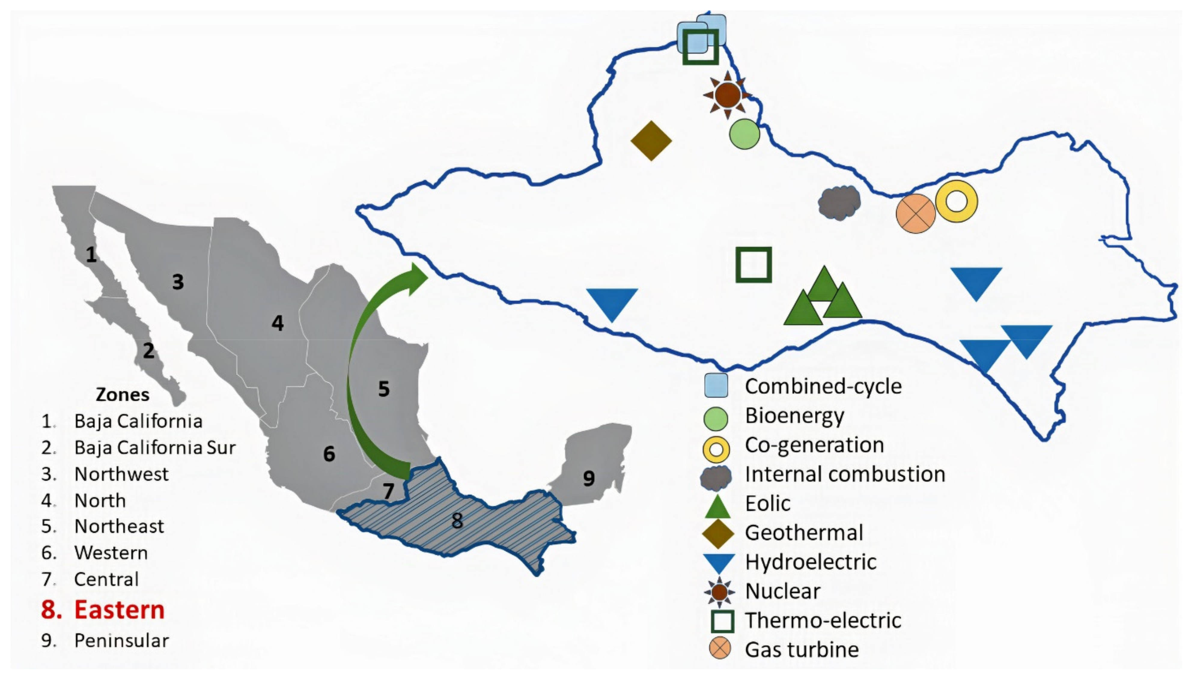
The energy distribution system in Mexico consists of nine zones, as shown in Figure 1. Each zone has its characteristics of supplying energy according to the requested demand [37].
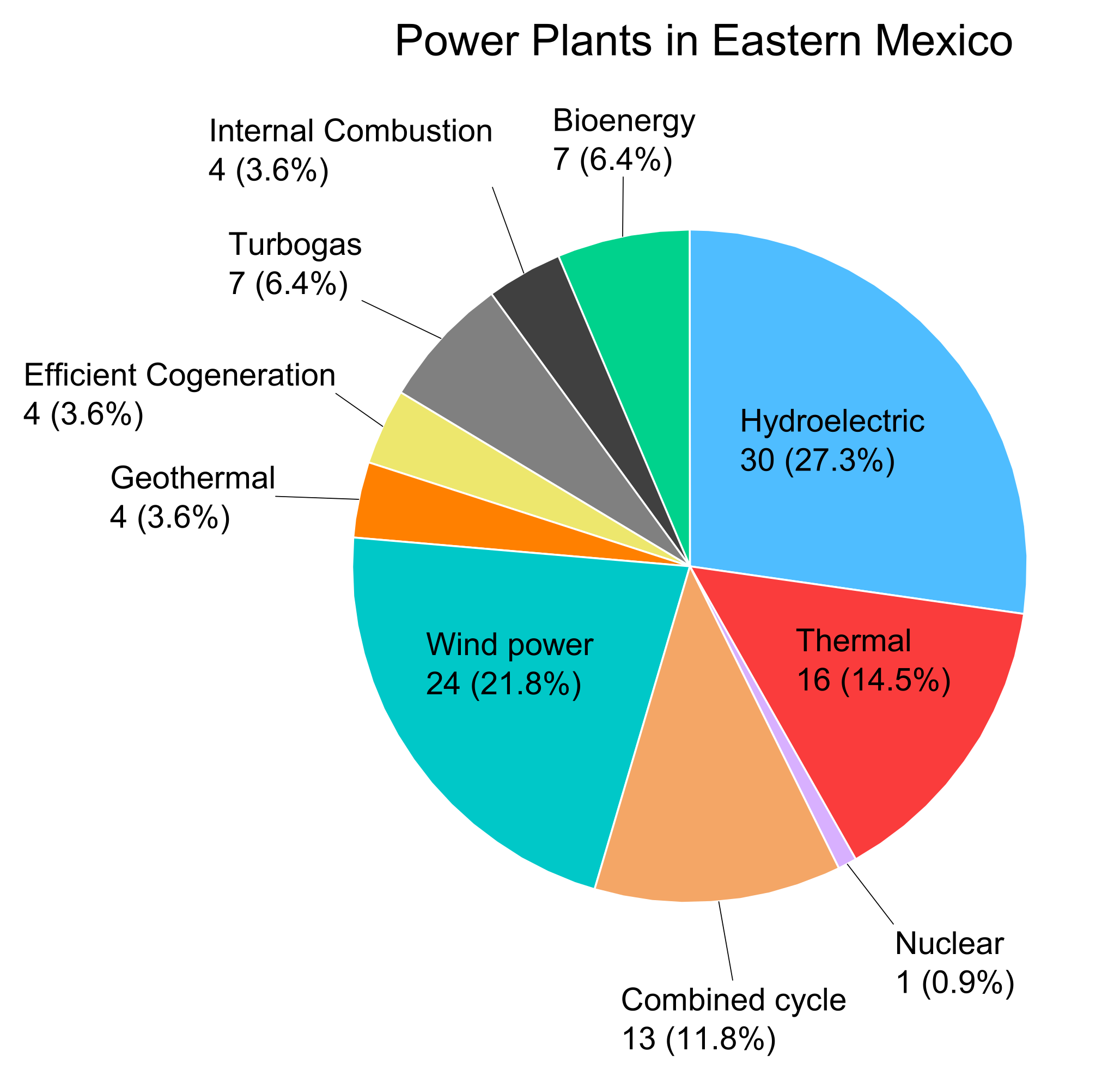
The eastern part of Mexico has 110 generation plants, of which the primary source is hydroelectric and wind energy, as shown in Figure 2. This feature is due to its geographical location and high wind potential.
As shown in Figure 2, the range of generation technologies permits a higher installed capacity in the zone according to the regional demand. This feature allows 22% of energy generation to contribute to the Mexico national requirements [37] and supply other areas such as the Central and Peninsular zones. In the Central Zone, the population density is around 899 inhabitants per km2. Big corporations established in this zone contribute to 27% of the country’s gross domestic product (GDP) [38]. Therefore, the energy demand is much higher compared to the supply capacity in the central zone. On the other hand, there is a high energy demand in the Peninsular Zone because it is a substantial touristic infrastructure [38]. Therefore, it is necessary to promote energy end-use efficiency and optimize energy resources in these zones. The following section describes the implemented model in our case study.
2. Materials and Methods
As we mentioned, economic dispatch is a mathematical model that aims to manage system resources. For our purposes, this model permits efficiently handling all power plant supplies in an interconnected network. The objective is to obtain the optimal combination in each generator’s contribution to satisfy the energy demand and minimize its generation costs. The modeling considerations incorporate real characteristic parameters of each of the plants to obtain useful results for decision-making. In the following, the proposed mathematical model is described.
2.1. Modeling for a Certain Time
In an electrical generation system, there are several plants with particular characteristics. These, concerning the central, are denoted by , that is . Where is the total number of generation plants in the system and each one works under certain limits. No plant can operate below the minimum operating power, which is described as:
where is the minimum power of the central and is a binary operating variable. If , it means that the central is working. When is multiplied by the minimum power, it will not be below its nominal value and is the optimal power to be generated by each plant. To exemplify these conditions, suppose we have a system of three plants and plant 1 has a minimum power of 45 MW, plant number two is 35 MW and plant 3 is 40 MW. Implementing these parameters in Equation (1), it remains:
On the other hand, no control unit can operate above the maximum operational power :
Similarly, if the plant is working, the power to be generated must not be exceeded. The power generated by each plant must satisfy the demand requested by the electrical distribution grid; therefore:
On the other hand, demand fulfillment generates individual costs which determine the total cost of generation, called . For this reason, resources must be correctly assigned to minimize them. Thus, the whole cost function is given as:
The first term indicates the fixed cost of plant and is the binary variable described above ( is working and is off). The term corresponds to the contribution of the cost assumed to be proportional to the production of the plant, where is the variable cost and the production for the plant . Besides, a plant also generates costs just for being stopped. This contribution is represented by the third term , where is the cost of having each plant stopped and is also a binary stop variable that takes the value 1 if plant stops and 0 indicates the opposite case.
This model describes the conditions to satisfy energy demand in a given time, limiting the power plants’ administration because it does not allow long-term planning. The following section describes the mathematical considerations in the modeling for time intervals to have a more significant representation in the resources assigned.
2.2. Model for Various Periods
The problem of scheduling power plants by periods consists of determining for the planning horizon both the start-up and shut-down of each power plant and the allocation of energy to be generated. These three parameters must satisfy the demand in each cycle of time, reduce costs, and comply with specific technical and operational safety restrictions in each plant . These planning horizons are divided into a day by time cycles. These time cycles are denoted by , so the planning horizon consists of the periods: , where is determined by the number of cycles defined in total for the study. Each of the power plants cannot operate below their minimum energy generation, being established for various periods such as:
where is the minimum energy to generate plant in period ; is the energy that plant will generate in period ; and is the binary variable described above. Suppose, for example, we have a system of three plants and three established periods, if we talk about the minimum energy to be generated in plant 2 in period 3 it is established as:
Similarly, the power plants cannot produce more than the established maximum energy ; then:
The energy to be produced in each plant in one period cannot increase abruptly in the immediately following period above a maximum quantity. This energy is known as the maximum load rise ramp , expressed as:
The difference between energy produced in the immediately following period and the current period’s energy must be less than or equal to the maximum rising ramp of of the plant . Similarly, no power plant can reduce its energy production under a limit called the maximum load descent ramp . So:
Additionally, it is convenient to define two conditions that allow setting the starting and braking for each plant, in order to have greater control of the costs that may be generated. For the first case, let us consider that a plant that is operating in a period is established to be in operation and a previous period is also in operation. In this case, it cannot start in period expressed as:
where is also a binary start-up variable, and if indicates the central is working in a period and for the opposite case. In the same way, if a plant is in operation, it cannot be stopped and vice versa, therefore:
where is the stop binary variable that indicates plant is stopped in period and when not; thus, it is possible to establish an equation that determines the state and allows these conditions to be fulfilled, given by:
To verify that the general conditions and any exchange are valid, consider the following particular example. Suppose that control unit 1 is stopped in period 1, but in the following period, it is in operation, which means that in period 2, it is going to start. Therefore it cannot be stopped in the same period 2. The equation for this situation is expressed:
To verify that this last situation is consistent under the proposed model, consider the case that the power plant was off in period 1 and remained off in period 2, which is obtained from Equation (12):
Thus, employing the example proposed in Equation (12), it is verified that all the variables describe the logic of possible states in the system. On the other hand, the proposed model must supply the demand in each period. In consequence:
where is the total demand to cover in period , the proposed Equations (5)–(12) are the restrictions inherent to each power plant in the system, where it is sought to reduce generation scabs by satisfying the demand established in Equation (13).
The cost minimization now considered in all time intervals must include all the regular electric power production plants’ programming. Therefore, it must be expressed in terms of all possible contributions:
where it is the sum of all the costs of the plants in each of the periods. The first term of Equation (14) incorporates the fixed cost of each generation plant. The second term associates the variable cost , considering that it is proportional to the plant’s production and directly related to the cost of fossil fuels. The next cost in this model is considered the start-up of a plant, where it is assumed to be constant throughout the periods. Finally, the fourth term of Equation (14) incorporates the cost , generated when a plant is off. As can be seen, each of the costs described is established according to the state parameters defined by the activation or shut-down binary , , , and , respectively.
The conditions established to satisfy the different energy demands in the time intervals allow long-term planning, maintaining the optimal distribution of resources and minimizing the total cost of generation from the model as shown in Table 1.
3. Implementation and Discussion of Results
The control area selected to carry out the study consists of 110 power plants that provide 16,992 MW of installed capacity with different technologies. The demand in the area has a value from 6750 MW to 8500 MW on average per hour, according to the National Center for Energy Control (known by its spanish accronim, CENACE) in Mexico.
From 110 power plants, we select 17 representative power plants which correspond to 57% of the area’s installed capacity. This selection maintains the proportionality of the installed capacity of the area by type of technology. These plants have characteristic parameters such as maximum energy () and minimum energy (), variable costs fixed cost , start-up costs , and shut-down costs () as is shown in Table 2.
For wind power plants, the maximum and minimum energy to be generated are obtained based on the statistics of the historical wind speed data of the place where they are located as reported by the Mexican ministry of energy [36]. The wind statistics are obtained through the Weibull probability density model, and in the same way with respect to hydroelectric plants, but it is a probability function of the flow and level they present.
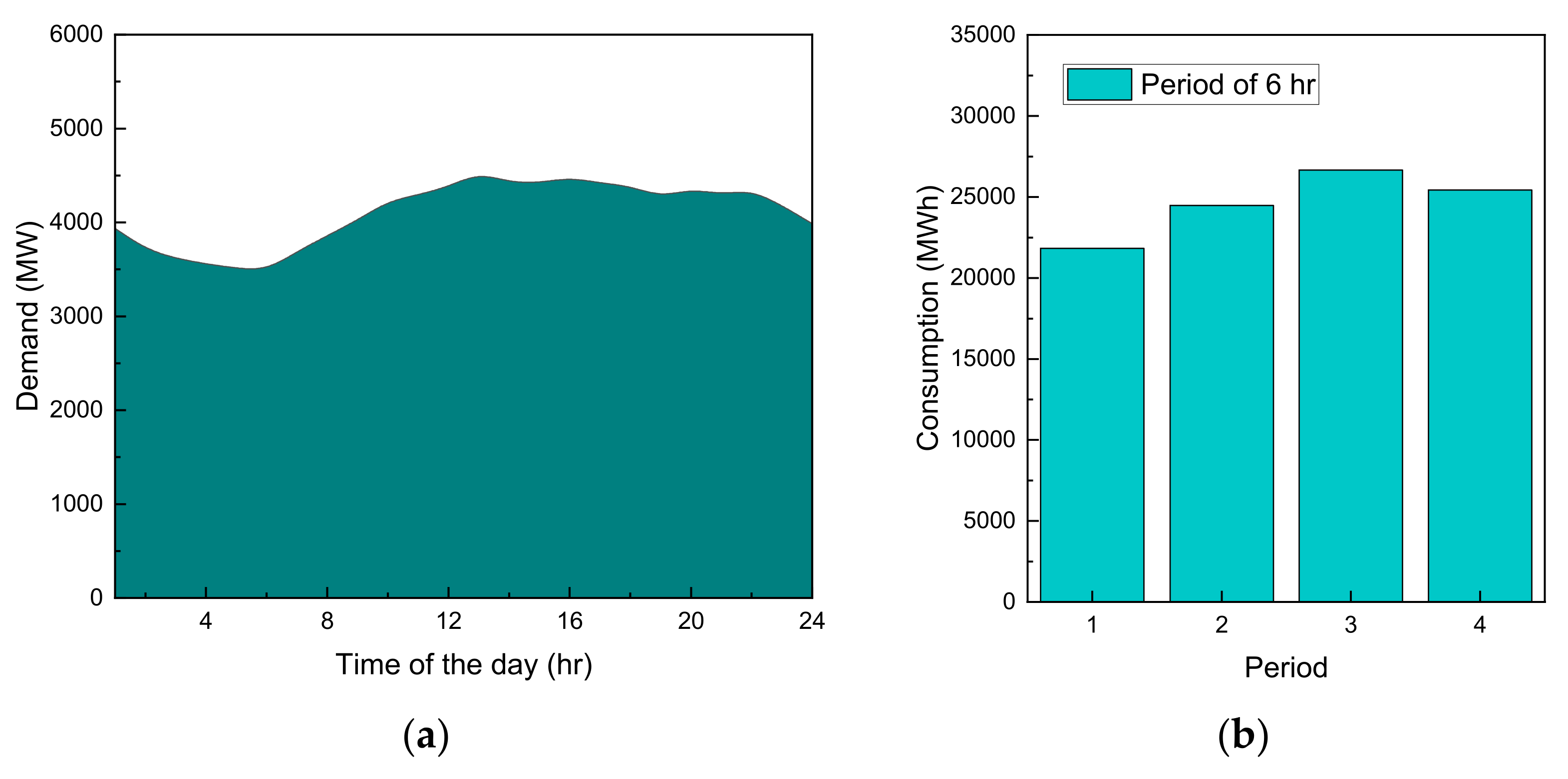
For the model’s implementation, it is necessary to indicate the requested demand in each period of the area, establishing 52% of the total demand for representing the study plants as shown in Figure 3a, and we are assuming 5% additional to compensate for generation losses that could be generated at the time of transmission, which means a total of 57% being established. Therefore, four periods were established in which each period consists of 6 h in duration, as reflected in Figure 3b. It is worth mentioning that these data are real and were provided by CENACE based on monitoring carried out every hour over a three-week interval.
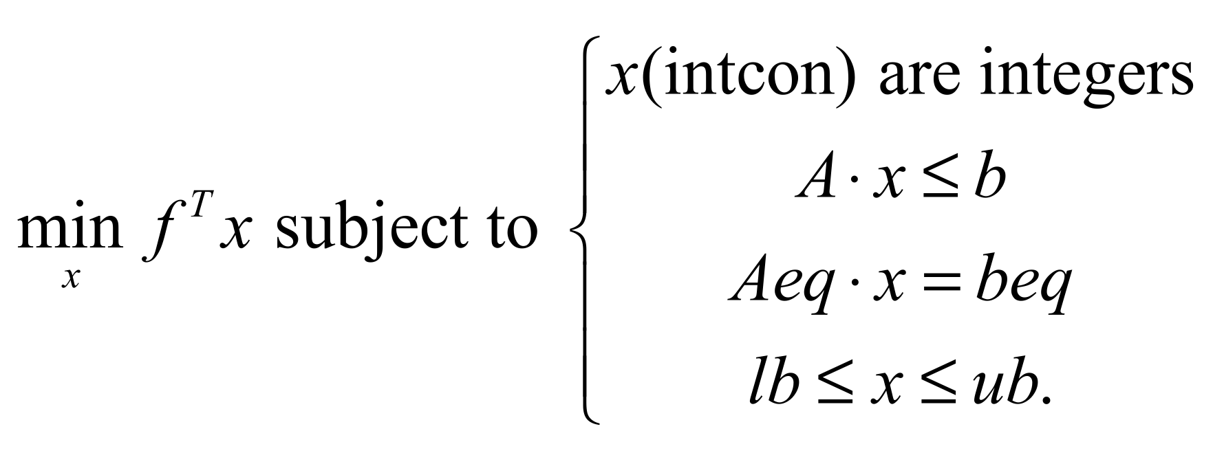
The model established by Equations (5)–(14) and applied to the geographical area described above was implemented using the MATLAB® programming tool, by means of the intlinprog function, which allows solving mixed-integer linear programming problems, and which has the structure as shown in Figure 4.
Where is a vector of the objective function, is a vector of the binary variables of the problem, is a matrix, with the values of the left side of the inequalities, and is the vector of the right side of the inequalities. is a matrix with the values on the left side of the model equations, is the right side of the equations, and are a vector with the maximum and minimum values of the variables. For the generation of these matrices and vectors, the proper values of each plant established in Table 1 are taken, obtaining the matrices with the following dimensions , , , , , , , and
Once the matrices of the system were defined, the results presented in Table 3, Table 4, Table 5 and Table 6 and Figure 5, Figure 6, Figure 7 and Figure 8 were obtained. In them, the values for each variable defined in each of the defined periods are indicated.
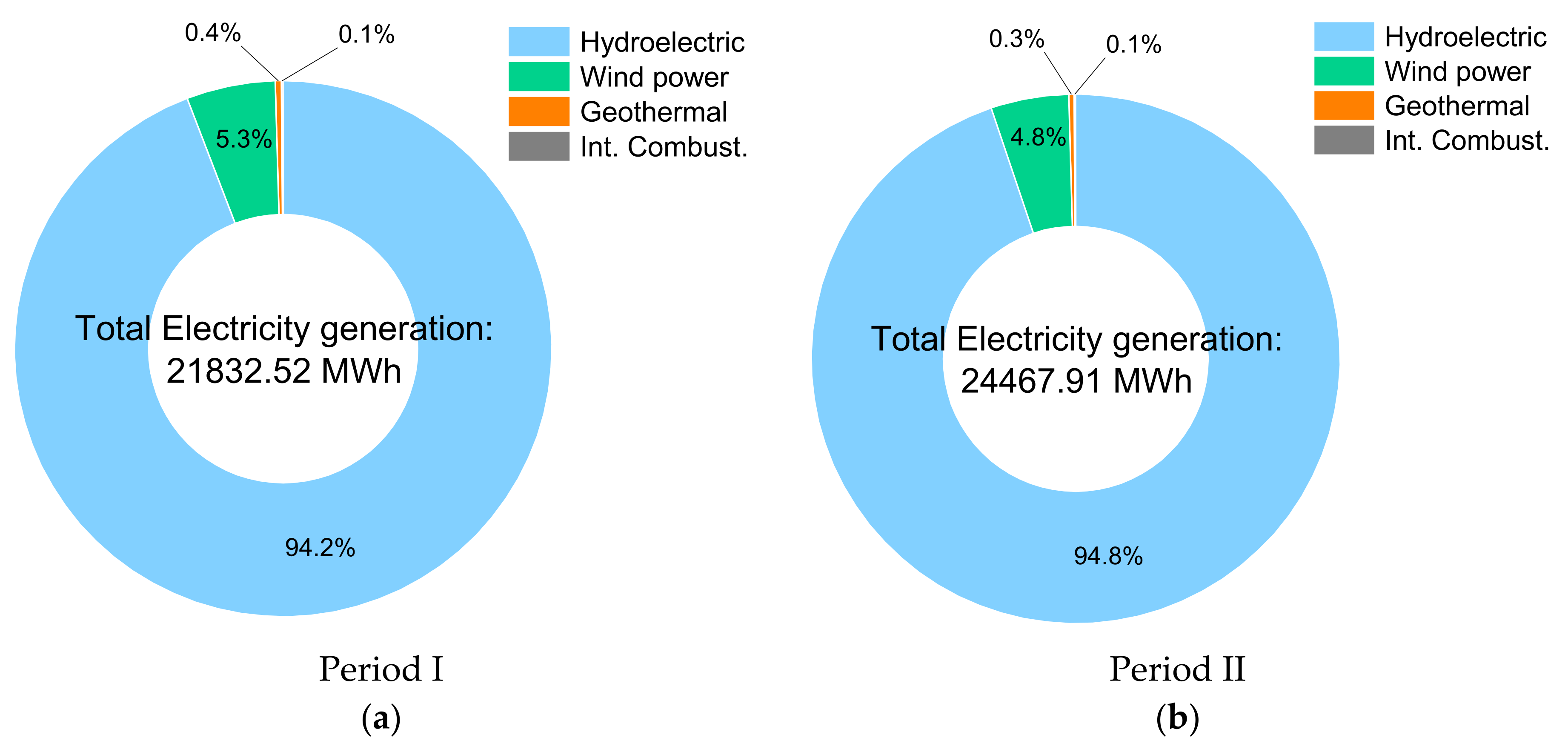
In the first period, identified from 00:00 to 06:00 h, an energy demand of 21,832.52 MWh was managed. This demand is the lowest of the four periods considered because they are the first hours of the day and, consequently, cover less human activity. The power plants contributing to related demand are from technologies such as internal combustion, wind, geothermal, and hydroelectric, the contributions of which make it optimal, as shown in Table 3 and Figure 5a.
Table 4 shows the model variables’ results in period 2, where the demand to be satisfied is 24,467.92 MWh, as shown in Figure 5b.
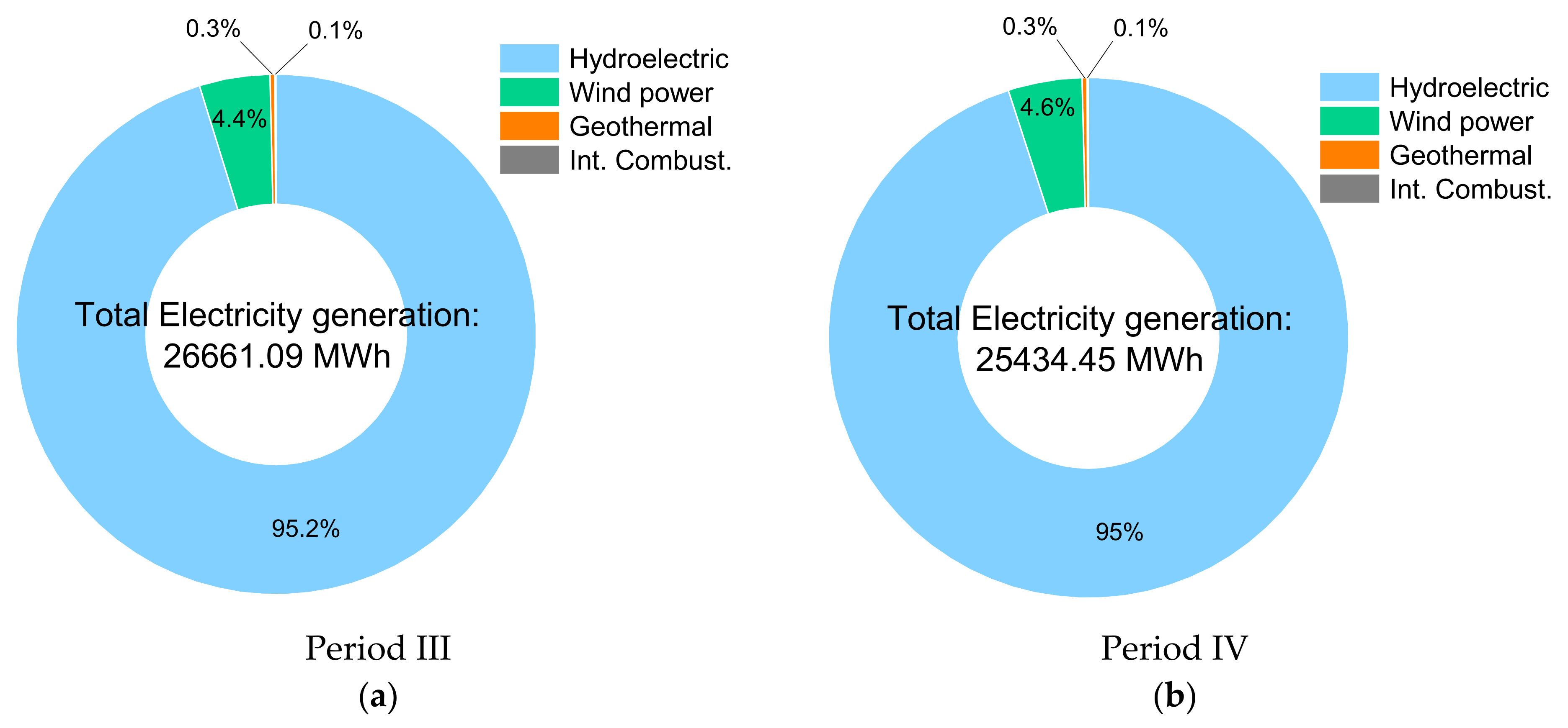
Additionally, in Period 3 (see Table 5 and Figure 6a), the demand to be satisfied is the highest of the four periods, corresponding to 26,661.1 MWh. Here, the power plants that contribute to cover most of the demand are wind and hydroelectric. This aspect can be an opportunity to incorporate clean technologies for the generation of energy that satisfies the requested demand.
Finally, in period 4, the demand to satisfy is 25,434.44 MWh; the results of which are produced by the model and are described in Table 6 and Figure 6b. It is in this period where the most significant contribution is observed from renewable energies. In this way, we can observe that the model complies with what is proposed because it satisfies the demand for the established periods.
Figure 7 shows the different plants that comprise the study carried out and the contributions of each one of them in the different periods established to satisfy the demand in each one.
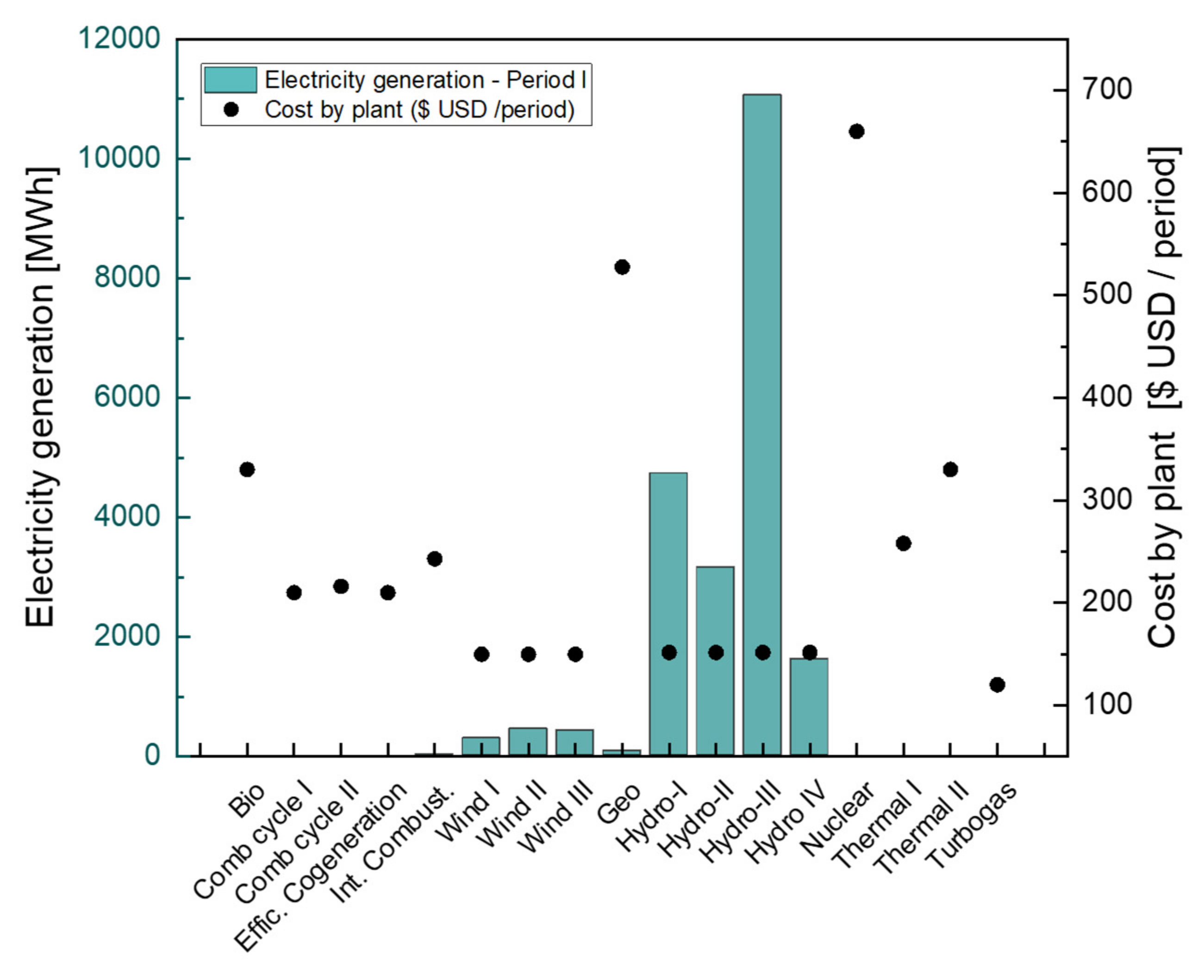
The costs obtained in period 1 are illustrated in Figure 8, which shows the behavior, and this trend continues in the following periods. The highest costs come from fossil fuel technology plants. This is mainly due to the various fossil fuels’ high variable costs and the various costs attributed to these technologies. The lowest costs are from clean generation sources because maintenance costs are lower and provide benefits for the ecosystem.
4. Conclusions
In this work, the optimization of an Economic Dispatch model for a power supply network located in Mexico’s eastern zone is presented. The established model incorporates real parameters and intrinsic restriction to each plant. The energy production of the renewable energy plants was estimated by means of probability functions according to the historical data of the location. The considerations incorporate the various types of generation costs and seek their minimization. This allows the state logic to be fulfilled at all times, as can be seen in Table 3, Table 4, Table 5 and Table 6; this is due to Equations (10)–(12), which do not allow a power plant to be off and on at the same time, as well as also that a plant does not start in a period when it was on in the previous period. In addition, all costs can be better accounted for by relating them to binary variables, such as the shutdown, operation, and start-up of a plant.
The results show a majority participation of clean energy plants during the study time period. The model shows the costs that each of the power plants has in period 1, and it reflects the lower costs of the power generation mix that contribute to satisfying the demand, being in this case a combination of clean energy plants. In contrast, the study shows that some non-operating fossil fuel plants generate even higher costs than renewable plants in operation.
The mathematical model could be an important tool in decision-making in plant planning and a diagnostic mode that allows visualizing those plants with very high costs when incorporating new electricity generation sources. In future works, longer periods of time should be addressed (one year) to obtain more significant results from the most suatible energy generation mix for the zone. Energy distribution will be incorporated due to the importance of power plants, location, and the loads due to the loss of lines at transmission and their capacities. In this way, there is a broader panorama to analyze the system as a decision-making tool.
Author Contributions
Conceptualization, I.S.-T. and R.F.D.-C.; methodology, E.L.; software, E.L. and R.F.D.-C.; validation, E.L., R.F.D.-C. and I.S.-T.; formal analysis, E.L., R.F.D.-C. and I.S.-T.; investigation, E.L.; resources, R.F.D.-C., data curation, E.L.; writing—original draft preparation, E.L.; writing—review and editing, R.F.D.-C. and I.S.-T.; visualization, E.L. and I.S.-T.; supervision, R.F.D.-C. and I.S.-T. All authors have read and agreed to the published version of the manuscript.
Funding
This research received no external funding.
Conflicts of Interest
The authors declare no conflict of interest.
References
- Kumar, Y.V.; Sivanagaraju, S.; Suresh, C.V. Analyzing the effect of dynamic loads on economic dispatch in the presence of interline power flow controller using modified BAT algorithm. J. Electr. Syst. Inf. Technol. 2016, 3, 45–67. [Google Scholar] [CrossRef] [Green Version]
- Hadera, H.; Ekström, J.; Sand, G.; Mäntysaari, J.; Harjunkoski, I.; Engell, S. Integration of production scheduling and energy-cost optimization using Mean Value Cross Decomposition. Comput. Chem. Eng. 2019, 129, 106436. [Google Scholar] [CrossRef]
- Ringwood, J.V.; Bofelli, D.; Murray, F.T. Forecasting Electricity Demand on Short, Medium and Long Time Scales Using Neural Networks. J. Intell. Robot. Syst. 2001, 31, 129–147. [Google Scholar] [CrossRef]
- Bruno, S.; Dellino, G.; La Scala, M.; Meloni, C. A Microforecasting Module for Energy Management in Residential and Tertiary Buildings. Energies 2019, 12, 1006. [Google Scholar] [CrossRef] [Green Version]
- Dong, L.; Liu, M.; Fan, S.; Pu, T. A Stochastic Model Predictive Control Based Dynamic Optimization of Distribution Network. In Proceedings of the 2018 IEEE Power & Energy Society General Meeting (PESGM), Portland, OR, USA, 5–10 August 2018; pp. 1–5. [Google Scholar]
- Chang, P.-C.; Fan, C.-Y.; Lin, J.-J. Monthly electricity demand forecasting based on a weighted evolving fuzzy neural network approach. Int. J. Electr. Power Energy Syst. 2011, 33, 17–27. [Google Scholar] [CrossRef]
- Kafazi, I.; Bannari, R.; Adib, I.; Nabil, H.; Dragicevic, T. Renewable energies: Modeling and optimization of production cost. Energy Procedia 2017, 136, 380–387. [Google Scholar] [CrossRef]
- Investigación de Operaciones. Available online: https://editorialpatria.com.mx/pdffiles/9786074386967.pdf (accessed on 3 June 2021).
- Caballero, J.A.; Grossmann, I.E. Una revisión del estado del arte en optimización. Revista Iberoam. Automática Inf. Ind. 2007, 4, 5–23. [Google Scholar] [CrossRef] [Green Version]
- Taha, H.A. Investigación de Operaciones, Novena ed.; Pearson Educación: Naucalpan de Juárez, Mexico, 2012; ISBN 978-607-32-0796-6. [Google Scholar]
- Somma, M.D.; Yanc, B.; Biancob, N.; Graditia, G.; Luhc, P.B.; Mongibelloa, L.; Naso, V. Design optimization of a distributed energy system through cost and exergy assessments. Energy Procedia 2017, 105, 2451–2459. [Google Scholar] [CrossRef]
- di Pilla, L.; Desogus, G.; Mura, S.; Ricciu, R.; Di Francesco, M. Optimizing the distribution of Italian building energy retrofit incentives with Linear Programming. Energy Build. 2016, 112, 21–27. [Google Scholar] [CrossRef]
- McLarty, D.; Panossian, N.; Jabbari, F.; Traverso, A. Dynamic economic dispatch using complementary quadratic programming. Energy 2019, 166, 755–764. [Google Scholar] [CrossRef]
- Arsuaga-Ríos, M.; Vega-Rodríguez, M.A. Multi-objective energy optimization in grid systems from a brain storming strategy. Soft Comput. 2014, 19, 3159–3172. [Google Scholar] [CrossRef]
- Arabali, A.; Ghofrani, M.B.; Etezadi-Amoli, M.; Fadali, M.S.; Baghzouz, Y. Genetic-Algorithm-Based Optimization Approach for Energy Management. IEEE Trans. Power Deliv. 2013, 28, 162–170. [Google Scholar] [CrossRef]
- He, G.; Yan, H.; Liu, K.; Yu, B.; Cui, G.; Zheng, J.; Pan, Y. An optimization method of multiple energy flows for CCHP based on fuzzy theory and PSO. In Proceedings of the 2017 IEEE Conference on Energy Internet and Energy System Integration (EI2), Beijing, China, 26–28 November 2017; pp. 1–6. [Google Scholar]
- Li, Y.; Yao, J.; Yao, D. An efficient composite simulated annealing algorithm for global optimization. In Proceedings of the IEEE 2002 International Conference on Communications, Circuits and Systems and West Sino Expositions, Chengdu, China, 29 June–1 July 2002; Volume 2, pp. 1165–1169. [Google Scholar]
- Toksarı, M.D. Ant colony optimization approach to estimate energy demand of Turkey. Energy Policy 2007, 35, 3984–3990. [Google Scholar] [CrossRef]
- Kawaguchi, S.; Fukuyama, Y. Reactive Tabu Search for Job-shop scheduling problems considering peak shift of electric power energy consumption. In Proceedings of the 2016 IEEE Region 10 Conference (TENCON), Singapore, 22–25 November 2016; pp. 3406–3409. [Google Scholar]
- Kumar, M.V.L.; Prasanna, H.A.M.; Ananthapadmanabha, T. An Artificial Bee Colony algorithm based distribution system state estimation including Renewable Energy Sources. In Proceedings of the 2014 International Conference on Circuits, Power and Computing Technologies [ICCPCT-2014], Nagercoil, India, 20–21 March 2014; pp. 509–515. [Google Scholar]
- Killian, M.; Zauner, M.; Kozek, M. Comprehensive smart home energy management system using mixed-integer quadratic-programming. Appl. Energy 2018, 222, 662–672. [Google Scholar] [CrossRef]
- Zio, E.; Baraldi, P.; Pedroni, N. Optimal power system generation scheduling by multi-objective genetic algorithms with preferences. Reliab. Eng. Syst. Safety 2009, 94, 432–444. [Google Scholar] [CrossRef]
- Rodzin, S.I. Smart Dispatching and Metaheuristic Swarm Flow Algorithm. J. Comput. Syst. Sci. Int. 2014, 53, 109–115. [Google Scholar] [CrossRef]
- Gallego Carrillo, M.; Pantrigo Fernández, J.J.; Duarte Muñoz, A. Metaheuriísticas; Dykinson: Madrid, Spain, 2007. [Google Scholar]
- Eren, Y.; Küçükdemiral, İ.B.; Üstoğlu, İ. Chapter 2—Introduction to Optimization. In Optimization in Renewable Energy Systems; Erdinç, O., Ed.; Butterworth-Heinemann: Oxford, UK, 2017; pp. 27–74. ISBN 9780081010419. [Google Scholar]
- Cardona, H.A.; Burgos, M.A.; González, J.W.; Isaac, I.A.; López, G.J. Aplicación en Matlab para la programación del despacho económico hidrotérmico. Rev. Investig. Aplicadas. 2012, 6, 42–53. [Google Scholar]
- Augustine, N.; Suresh, S.; Moghe, P.; Sheikh, K. Economic dispatch for a microgrid considering renewable energy cost functions. In Proceedings of the 2012 IEEE PES Innovative Smart Grid Technologies (ISGT), Washington, DC, USA, 16–20 January 2012; pp. 1–7. [Google Scholar]
- Ramanathan, R. Emission constrained economic dispatch. IEEE Trans. Power Syst. 1994, 9, 1994–2000. [Google Scholar] [CrossRef]
- Muslu, M. Economic dispatch with environmental considerations: Tradeoff curves and emission reduction rates. Electr. Power Syst. Res. 2004, 71, 153–158. [Google Scholar] [CrossRef]
- Gaing, Z.-L. Particle swarm optimization to solving the economic dispatch considering the generator constraints. IEEE Trans. Power Syst. 2003, 18, 1187–1195. [Google Scholar] [CrossRef]
- Meiqin, M.; Meihong, J.; Wei, D.; Chang, L. Multi-objective economic dispatch model for a microgrid considering reliability. In Proceedings of the 2nd International Symposium on Power Electronics for Distributed Generation Systems Hefei, Hefei, China, 16–18 June 2010; pp. 993–998. [Google Scholar] [CrossRef]
- Wang, Y.; An, Y.; Xi, F.; Yao, J.; Wei, Q. Multi-Objective Optimal Operation of Micro-Grid Based on Demand Side Management. J. Phys. Conf. Ser. 2018, 1087, 062009. [Google Scholar] [CrossRef]
- Zhang, Y.; Gatsis, N.; Giannakis, G. Robust Energy Management for Microgrids With High-Penetration Renewables. IEEE Trans. Sustain. Energy 2013, 4, 944–953. [Google Scholar] [CrossRef] [Green Version]
- Liu, D.; Li, Q.; Yuan, X. Economic and optimal dispatching of power microgrid with renewable energy. In Proceedings of the 2014 China International Conference on Electricity Distribution (CICED), Shenzhen, China, 23–26 September 2014; pp. 16–20. [Google Scholar]
- Secretaria de Gobernación. Marco Legal y Regulatorio del Sector Energético en MÉXICO. Available online: https://www.gob.mx/cms/uploads/attachment/file/116455/1665.pdf (accessed on 3 June 2021).
- Secretaría de Energía. El Gobierno de México Fortalece el Sistema Eléctrico Nacional. Available online: https://www.gob.mx/sener/articulos/el-gobierno-de-mexico-fortalece-el-sistema-electrico-nacional (accessed on 3 June 2021).
- Centro Nacional de Control de Energía (CENACE). Demandas del Sistema Eléctrico Nacional. Available online: https://www.cenace.gob.mx/Paginas/Publicas/Info/DemandaRegional.aspx (accessed on 3 June 2021).
- Instituto Nacional de Estadística y Geografía (INEGI). Producto Interno Bruto por Entidad Federativa 2019. Available online: https://www.inegi.org.mx/contenidos/saladeprensa/boletines/2020/OtrTemEcon/PIBEntFed2019.pdf (accessed on 3 June 2021).
- The Mexican National Institute for the Acess to Information. Ministry of Energy. Application Number: 0001800090519. 2019. Available online: https://buscador.plataformadetransparencia.org.mx/web/guest/buscadornacional?buscador=0001800090519&coleccion=5 (accessed on 3 June 2021).
- MathWorks. Mixed-Integer Linear Programming (MILP). Available online: https://www.mathworks.com/help/optim/ug/intlinprog.html?s_tid=srchtitle (accessed on 3 June 2021).
Figure 1.
Mexican Electric System denoted by zones. The zone of interest is shaded (zone 8). [34].
Figure 1.
Mexican Electric System denoted by zones. The zone of interest is shaded (zone 8). [34].

Figure 2.
Classification of generation plants in the Eastern Zone of Mexico according to technology used [37].
Figure 2.
Classification of generation plants in the Eastern Zone of Mexico according to technology used [37].

Figure 3.
The behavior of demand in the Eastern Zone. (a) The corresponding demand in the Eastern Zone per hour. (b) Consumption accross periods of 6 h.
Figure 3.
The behavior of demand in the Eastern Zone. (a) The corresponding demand in the Eastern Zone per hour. (b) Consumption accross periods of 6 h.

Figure 4.
Intlinpro function syntax from MATLAB® [40].
Figure 4.
Intlinpro function syntax from MATLAB® [40].

Figure 5.
Generation and Energy in periods 1 and 2. (a) Period 1. (b) Period 2.

Figure 6.
Generation and Energy in periods 3 and 4. (a) Period 3. (b) Period 4.

Figure 7.
Contribution of energy generation by each plant of the study in the periods.

Figure 8.
Electricity generation and Energy Costs for period 1.


Table 1.
Model equations.
| Minimum Energy |
|---|
| Maximum Energy |
| Maximum Load Rise Ramp |
| Maximum Load Descent Ramp |
| Start |
| On/Stop |
| State |
| Demand |
Table 2.
Parameters of the Electric Power Plants [39].
Table 2.
Parameters of the Electric Power Plants [39].
| Central | (MWh) | (MWh) | ||||
|---|---|---|---|---|---|---|
| 1. Bioenergy | 295.14 | 78.75 | 3.94 | 265.524 | 0 | 330 |
| 2. Combined cycle | 2883.9 | 742.5 | 2.72 | 92.28 | 0 | 210 |
| 3. Combined cycle | 5721.06 | 1474.5 | 2.69 | 90.174 | 0 | 216 |
| 4. Efficient Cogeneration | 2138.28 | 551.1 | 2.73 | 93.318 | 108.3 | 210 |
| 5. Internal Combustion | 86.22 | 23.55 | 3.16 | 168.264 | 108.3 | 258 |
| 6. Wind power | 294.9048 | 246 | 0 | 149.778 | 0 | 240 |
| 7. Wind power | 450.4491 | 375.75 | 0 | 149.778 | 0 | 240 |
| 8. Wind power | 420.7788 | 351 | 0 | 149.778 | 0 | 240 |
| 9. Geothermal | 301.98 | 80.4 | 0.06 | 522.708 | 0 | 270 |
| 10. Hydroelectric | 4728.24 | 1350 | 0 | 151.464 | 0 | 246 |
| 11. Hydroelectric | 3152.16 | 900 | 0 | 151.464 | 0 | 246 |
| 12. Hydroelectric | 12,608.64 | 3600 | 0 | 151.464 | 0 | 246 |
| 13. Hydroelectric | 5673.888 | 1620 | 0 | 151.464 | 0 | 246 |
| 14. Nuclear power plant | 8742.9 | 2265 | 2.25 | 588 | 0 | 660 |
| 15. Thermal | 2001.3 | 525 | 2.2 | 170.862 | 472.86 | 258 |
| 16. Thermal | 647.64 | 172.8 | 3.94 | 265.524 | 468.6 | 330 |
| 17. Turbogas | 715.5 | 181.05 | 4.19 | 51.102 | 216.6 | 120 |
Table 3.
Results of Period 1.
| Central | Power to Be Generated in 6 h | On | Start | Stop |
|---|---|---|---|---|
| 1. Bioenergy | 0 | 0 | 0 | 1 |
| 2. Combined cycle | 0 | 0 | 0 | 1 |
| 3. Combined cycle | 0 | 0 | 0 | 1 |
| 4. Efficient Cogeneration | 0 | 0 | 0 | 1 |
| 5. Internal Combustion | 23.55 | 1 | 0 | 0 |
| 6. Wind power | 294.9048 | 1 | 0 | 0 |
| 7. Wind power | 450.4491 | 1 | 0 | 0 |
| 8. Wind power | 420.7788 | 1 | 0 | 0 |
| 9. Geothermal | 80.4 | 1 | 0 | 0 |
| 10. Hydroelectric | 4728.24 | 1 | 0 | 0 |
| 11. Hydroelectric | 3152.16 | 1 | 0 | 0 |
| 12. Hydroelectric | 11062.0373 | 1 | 0 | 0 |
| 13. Hydroelectric | 1620 | 1 | 0 | 0 |
| 14. Nuclear power plant | 0 | 0 | 0 | 1 |
| 15. Thermal | 0 | 0 | 0 | 1 |
| 16. Thermal | 0 | 0 | 0 | 1 |
| 17. Turbogas | 0 | 0 | 0 | 1 |
Table 4.
Results of Period 2.
| Central | Power to Be Generated in 6 h | On | Start | Stop |
|---|---|---|---|---|
| 1. Bioenergy | 0 | 0 | 0 | 1 |
| 2. Combined cycle | 0 | 0 | 0 | 1 |
| 3. Combined cycle | 0 | 0 | 0 | 1 |
| 4. Efficient Cogeneration | 0 | 0 | 0 | 1 |
| 5. Internal Combustion | 23.55 | 1 | 0 | 0 |
| 6. Wind power | 294.91 | 1 | 0 | 0 |
| 7. Wind power | 450.45 | 1 | 0 | 0 |
| 8. Wind power | 420.78 | 1 | 0 | 0 |
| 9. Geothermal | 80.4 | 1 | 0 | 0 |
| 10. Hydroelectric | 4728.24 | 1 | 0 | 0 |
| 11. Hydroelectric | 3152.16 | 1 | 0 | 0 |
| 12. Hydroelectric | 12,608.64 | 1 | 0 | 0 |
| 13. Hydroelectric | 2708.79 | 1 | 0 | 0 |
| 14. Nuclear power plant | 0 | 0 | 0 | 1 |
| 15. Thermal | 0 | 0 | 0 | 1 |
| 16. Thermal | 0 | 0 | 0 | 1 |
| 17. Turbogas | 0 | 0 | 0 | 1 |
Table 5.
Results of period 3.
| Central | Power to Be Generated in 6 h | On | Start | Stop |
|---|---|---|---|---|
| 1. Bioenergy | 0 | 0 | 0 | 1 |
| 2. Combined cycle | 0 | 0 | 0 | 1 |
| 3. Combined cycle | 0 | 0 | 0 | 1 |
| 4. Efficient Cogeneration | 0 | 0 | 0 | 1 |
| 5. Internal Combustion | 23.55 | 1 | 0 | 0 |
| 6. Wind power | 294.91 | 1 | 0 | 0 |
| 7. Wind power | 450.45 | 1 | 0 | 0 |
| 8. Wind power | 420.78 | 1 | 0 | 0 |
| 9. Geothermal | 80.4 | 1 | 0 | 0 |
| 10. Hydroelectric | 4728.24 | 1 | 0 | 0 |
| 11. Hydroelectric | 3152.16 | 1 | 0 | 0 |
| 12. Hydroelectric | 12,608.64 | 1 | 0 | 0 |
| 13. Hydroelectric | 4901.96 | 1 | 0 | 0 |
| 14. Nuclear power plant | 0 | 0 | 0 | 1 |
| 15. Thermal | 0 | 0 | 0 | 1 |
| 16. Thermal | 0 | 0 | 0 | 1 |
| 17. Turbogas | 0 | 0 | 0 | 1 |
Table 6.
Results of period 4.
| Central | Power to Be Generated in 6 h | On | Start | Stop |
|---|---|---|---|---|
| 1. Bioenergy | 0 | 0 | 0 | 1 |
| 2. Combined cycle | 0 | 0 | 0 | 1 |
| 3. Combined cycle | 0 | 0 | 0 | 1 |
| 4. Efficient Cogeneration | 0 | 0 | 0 | 1 |
| 5. Internal Combustion | 23.55 | 1 | 0 | 0 |
| 6. Wind power | 294.91 | 1 | 0 | 0 |
| 7. Wind power | 450.45 | 1 | 0 | 0 |
| 8. Wind power | 420.78 | 1 | 0 | 0 |
| 9. Geothermal | 80.4 | 1 | 0 | 0 |
| 10. Hydroelectric | 4728.24 | 1 | 0 | 0 |
| 11. Hydroelectric | 3152.16 | 1 | 0 | 0 |
| 12. Hydroelectric | 12,608.64 | 1 | 0 | 0 |
| 13. Hydroelectric | 3675.32 | 1 | 0 | 0 |
| 14. Nuclear power plant | 0 | 0 | 0 | 1 |
| 15. Thermal | 0 | 0 | 0 | 1 |
| 16. Thermal | 0 | 0 | 0 | 1 |
| 17. Turbogas | 0 | 0 | 0 | 1 |
Publisher’s Note: MDPI stays neutral with regard to jurisdictional claims in published maps and institutional affiliations. |
© 2021 by the authors. Licensee MDPI, Basel, Switzerland. This article is an open access article distributed under the terms and conditions of the Creative Commons Attribution (CC BY) license (https://creativecommons.org/licenses/by/4.0/).
Share and Cite
MDPI and ACS Style
López, E.; Domínguez-Cruz, R.F.; Salgado-Tránsito, I. Optimization of Power Generation Grids: A Case of Study in Eastern Mexico. Math. Comput. Appl. 2021, 26, 46. https://0-doi-org.brum.beds.ac.uk/10.3390/mca26020046
AMA Style
López E, Domínguez-Cruz RF, Salgado-Tránsito I. Optimization of Power Generation Grids: A Case of Study in Eastern Mexico. Mathematical and Computational Applications. 2021; 26(2):46. https://0-doi-org.brum.beds.ac.uk/10.3390/mca26020046
Chicago/Turabian StyleLópez, Esmeralda, René F. Domínguez-Cruz, and Iván Salgado-Tránsito. 2021. "Optimization of Power Generation Grids: A Case of Study in Eastern Mexico" Mathematical and Computational Applications 26, no. 2: 46. https://0-doi-org.brum.beds.ac.uk/10.3390/mca26020046