
Review of Multi-Physics Modeling on the Active Magnetic Regenerative Refrigeration


Département ENERGIE, FEMTO-ST, CNRS, University Bourgogne Franche-Comté, F90000 Belfort, France
*
Author to whom correspondence should be addressed.
Math. Comput. Appl. 2021, 26(2), 47; https://0-doi-org.brum.beds.ac.uk/10.3390/mca26020047
Submission received: 20 April 2021
/
Revised: 31 May 2021
/
Accepted: 13 June 2021
/
Published: 15 June 2021
(This article belongs to the Special Issue Characterization of Magnetocaloric Devices and Materials through Mathematical Models)
Abstract
:Compared to conventional vapor-compression refrigeration systems, magnetic refrigeration is a promising and potential alternative technology. The magnetocaloric effect (MCE) is used to produce heat and cold sources through a magnetocaloric material (MCM). The material is submitted to a magnetic field with active magnetic regenerative refrigeration (AMRR) cycles. Initially, this effect was widely used for cryogenic applications to achieve very low temperatures. However, this technology must be improved to replace vapor-compression devices operating around room temperature. Therefore, over the last 30 years, a lot of studies have been done to obtain more efficient devices. Thus, the modeling is a crucial step to perform a preliminary study and optimization. In this paper, after a large introduction on MCE research, a state-of-the-art of multi-physics modeling on the AMRR cycle modeling is made. To end this paper, a suggestion of innovative and advanced modeling solutions to study magnetocaloric regenerator is described.
1. Introduction
1.1. General Context
In order to reduce greenhouse gas emissions and to decrease the carbon footprint, it is necessary to develop an alternative to the most polluting technologies. Among these technologies, the heating and cooling devices for a large part of the greenhouse gas emissions represent about 17% of the global electricity consumption [1]. This demand will increase in the next few years. In the current context, it is important to reduce this part of the consumption. Indeed, current cooling devices use refrigerant fluids such as hydrofluocarbons or more recently hydrochlorofluocarbons which are very polluting and harmful. For this reason, innovative studies for alternative refrigerants are performed [2,3]. To solve these problems, the AMRR seems to be a good alternative and one of the most promising technologies to replace actual cooling and heat pumping devices operating at room temperature [4].
The magneto-thermal effect was demonstrated by Gilbert (1600) [5], by showing the influence of temperature on the magnetic performance of an iron wire. The MCE was discovered by Warburg (1881) [6] and explained by Weiss and Picard (1918) [7]. First applications of MCE have been used for refrigeration, which is the most appropriate field for this phenomenon. In 1926, Debye proved that the MCE could be used to reach the 0 K with a cooling device [8]. One of the first devices was made by Giauque and MacDougall (1933) [9]. The first prototype operating around room temperature was developed by Brown (1976) [10]. Interest in this technology has increased significantly over the last 30 years and many prospects are being considered [11]. Other applications such as heat pumping are possible to exploit this effect, as showed by Tishin and Spichkin (2014) [12]. Recently, Kitanovski (2020) [13] reviewed the historical progress of this technology.
Throughout an adiabatic process, the MCE results from the change of the MCM temperature when they are subjected to a magnetic field variation. The magnetization, induced by (electro)magnet, increases the material temperature. This is a reversible effect. When the material is removed from the magnetic field, a decrease of the material temperature is induced. This effect is maximal around the Curie temperature of the material. Indeed, one of the most popular materials for near room temperature applications is the Gadolinium (Gd) (Figure 1) with a Curie temperature of 293 K. Despite its good characteristics, Gd can generate a temperature difference of 3 K under a magnetic field of 1 T. However, for applications at typical room temperatures, MCE alone is insufficient to be competitive with actual device.
To increase the temperature differences, it is necessary to develop devices that will perform AMRR cycles. This regenerator exchanges heat with a crossing fluid that circulates between two external heat sources (cold and hot). This heat transfer between these lasts increases the difference of their temperature. This type of cycle is called AMRR cycle [16]. To increase the efficiency, it is also possible to realize cascade systems consisting in several interconnected regenerators connected by heat sources [17]. However, it is necessary to technically and economically improve this technology, as well as the current devices, for a better commercialization. A scientific and technological breakthrough is needed to design a device with such feasibility and performance.
The modeling is an important step in the design of new devices. An efficient model permits to make several investigations to earn time and to increase efficiency of a device. For this review, the choice is made to focus the investigations on analytical modeling and on mathematical models solved with numerical software (semi-analytical). The investigated model can be one-dimensional (1-D), two-dimensional (2-D), or three-dimensional (3-D). In the literature, a previous review has already been done on modeling by Nielsen (2011) [18] and more recently in the PhD thesis of Plait (2019) [19]. Only models with a direct study on the AMRR cycles are described. They consider a regenerator exchanging heat fluxes with a liquid. These models consider at least the thermal and the fluidic effects.
This article shows the importance of the modeling for studies and improvements of new and future devices using MCE. It focuses on the advantages of a new type of modeling applied to magnetic refrigeration. It begins with a state-of-the-art of the existing AMRR modeling in the scientific literature. A review of modeling applied to magnetic, thermodynamic, fluidic, and thermomagnetic phenomena is made and compared to the current state of the AMRR modeling. Then, a conclusion with an overview on next works on the AMRR modeling is made. It is particularly shown that the (semi-)analytical modeling is one of the promising ways to obtain optimized efficiencies for AMRR devices in the future.
1.2. Material and Magnetocaloric Effect Modeling
Many investigations are made on the regenerator geometry and its structure. Concerning this last, it is more effective to have multi-layered (multi-stage) regenerator [20]. The type of material is also important. The studies of new MCM alloys are a key point to increase the performances of AMRR device. Indeed, a more performant MCM produces a higher temperature span for a same flux density. Many alloys are investigated to find new materials [21]. Recently, Ram et al. (2018) [22] reviewed a large amount of MCMs (i.e., manganite, composites and alloyed materials, spinel ferrites). They highlighted the composition and characteristics of each material they identified (i.e., magnetic entropy change, Curie temperature, field change, relative cooling power). They can be classified in two groups according to their magnetic phase transition, first-order or second order phase transition MCM. These magnetic phase transitions influence the material behavior under a magnetic field [4] (Figure 2).
A first order material is characterized by high variations of entropy and magnetization with temperature. The inconvenient is that this effect may be clouded for a very short temperature range. A second order material can be used on a larger temperature range, but the effect would then be less important. Some materials have both advantages for first- and second-order magnetic phase transition. These materials permit to obtain a giant MCE. Pecharsky and Gschneider showed for the first time in 1997 the giant MCE in Gd5(Si2Ge2) with a Curie temperature of 276 K [23].
The regenerator shape is very important and is directly responsible for device efficiency. Plenty of geometric shapes allowing to have an optimized heat transfer between the solid and the fluid should be considered. There are many regenerator geometries available: (i) micro-channel [24], (ii) packed bed of spheres [24], (iii) powder [25], (iv) cylinders [25], (v) honeycomb shape [26], (vi) parallel plates [27], (vii) flakes particles [28], (viii) thin ribbon [29], (ix) sheets [30].
Research laboratories carry out studies on materials. Some of them are described below. Few papers focus in the investigation on the demagnetization effect in materials. A model developed by Shir et al. (2004) [31] was made to study magnetization and demagnetization. The model can be used to optimize the design of an AMRR and to determine the temperature evolution of the MCM. Peksoy and Rowe (2005) [32] studied this effect with a 2-D numerical model. They investigated a two layered AMRR composed of Gd and alloy of GdTb (Terbium). They highlighted the importance to reduce the demagnetization effect to increase the efficiency of magnetic cycles, especially on the regenerator edge where the demagnetization is important. Also, Rowe and Tura (2008) [33] developed a 2-D numerical model with the finite-element method (FEM) to study the demagnetization effect. They demonstrated the importance of using passive magnetic material to decrease the demagnetization effects and to increase the performance of the AMRR. Huang and Teng (2004) [34] developed an evaluation model by the algorithms derivation procedures to make preliminary analysis in the design of magnetic refrigerator. The model was composed of the related term to the magnetism, entropy and the free energy. The input of the model is the entropy. The output is the temperature span generated by the studied system. The model has been validated by the comparison with the simulation of Ericsson and Brayton cycles.
Von Ranke et al. (2005) [35] proposed an analytical study about the board MCE observed for MnAs alloys under pressure and discovered by Gama et al. (2004) [36]. According to them, this effect finds its origin in the entropy variation coming from the lattice through the magneto-elastic coupling. They want to understand this effect and its contribution on the MCE. Their analytical model enabled observation of the entropy and the magnetization variations according to the temperature (Figure 3). With their model and in order to make an adapted study of the MCE, they pointed out the necessity to consider the coupling between magnetic and crystal lattice. Indeed, this relation is a key point to estimate the variation of the MCM entropy. They performed a parametric study and investigated several sets of parameters to observe how the total entropy change is affected by the lattice entropy. The sets are composed of two parameters (i.e., for the set 1: γ = 0, η = 0). The parameter γ is the Grüneisen parameter and η is a parameter which controls the order of the magnetic phase transitions.
Kawanami et al. (2006) [37] studied the optimization of an experimental device. The device uses air as heat transfer fluid. The rate and the temperature of air flow at the entrance of the device are regulated. The considered magnetic working substance is Gd packed chips. The aim is to find an optimal behavior of the device. In order to achieve their optimization, they developed an analytical model to determine the evolutions of the air and the MCM temperatures. They measured and simulated the evolution of the air temperature with the air flow rate, in the phase of (de)magnetization (Figure 4). The analytical and experimental results show differences because the used Gd is composed with iron and aluminum that have impurities. Gschneider (1993) [38] showed the importance of high purities on the material performances. They made other simulations to observe the temperatures evolution of the air and the Gd during some cycles. The device and the analytical model are still simple, but they highlighted the MCE and the importance of working near the Curie temperature of the MCM.
F. Allab et al. (2006) [39] developed a 2-D model considering the magnetic flux density distribution and the interaction between the magnetic source and the MCM. They studied the magnetic flux density distribution for two types of systems: (i) a Halbach cylinder (the simple and double structures are compared) constituted of permanent magnets (PMs), and (ii) a mixed C-structure made of PMs and ferromagnetic yokes. They have also studied the magnetic force distribution in another structure. This last was a simple geometry, composed by two PMs and ferromagnetic materials and an air-gap between them. The MCM moves inside and outside the air-gap during the simulation. They have compared and analyzed the magnetic force distribution during the magnetization and demagnetization phases. The magnetic flux density and force calculations have been validated using a 3-D FEM with the Flux3D® software. The comparison showed a good accuracy of their model (Figure 5). Other papers have conducted a study on the optimization of Halbach cylinders, such as Bjørk et al. (2008) [40]. The authors showed the interest of using Halbach cylinders as a magnetic field source to increase the efficiency of magnetic cooling. They investigated the optimal design of a Halbach cylinder to achieve the best magnetic cooling efficiency with MCM.
More recently, Fortkamp et al. (2017) [41] proposed a parametric study on the performance of two-poles nested Halbach cylinders for the AMRR and heat pumping applications. In order to perform this parametric analysis, they made an analytical model by extending the single-cylinder solution of Bjørk et al. [42]. This analytical model solves the Maxwell’s equations for the magnetic field and flux density. Then, results of the analytical model have been validated with numerical simulations on COMSOL Multiphysics®. The system is composed of two Halbach cylinders of NdFeB PMs, which generates a magnetic field between them. The AMRR is disposed in the air-gap between the cylinders. The calculations aim to observe the magnetic flux density as a function of different parameters as the magnetic field and flux as well as the geometric parameters. Indeed, a high magnetic flux density involves high system efficiency. The authors searched the best combination of geometric parameters to improve the magnetic flux density (Figure 6). They studied how the geometric parameters influence the efficiency of the device by observing the variation of the magnetic circuit characterization parameter . A device with a high value of means that it can provide a large temperature variation.
Hess et al. (2020) [43] created an empirical model of materials to study a first-order MCM La(Fe,Mn,Si)13 alloy-based. They used a modified Cauchy-Lorentz function as a base function of the specific heat capacity. The model of the relevant equations is determined from the specific heat capacity also function of the temperature and the magnetic field. The performances of the model are compared to measured data (Figure 7). According to the authors, a better agreement with measured data can be achieved through more degrees of liberty of the model. Nevertheless, it also increases the complexity of the model. The model can be implemented in a more global model to simulate cooling devices using a first-order MCM. Then the chosen compatibility seems to be a best way compared to the obtained accuracy of the model integrated into a complete modeling system. Their model gives an analytical description of the thermal behavior of the caloric material. Previously, another model has been developed by Hess et al. (2018) [44].
1.3. AMRR Device
Many reviews and states-of-the-art on the experimental devices are available: Yu et al. (2010) [45], Kitanovski et al. (2015) [46], Trevizoli et al. (2016) [47], and Greco et al. (2019) [48]. Overview tables in [46] and [48] summarize the characteristics of each existing device (i.e., MCM used, the magnetic field source, the year of production, the type of devices, the performances...). There are three types of devices: rotary, linear, and static according the magnetic field source and the regenerator. The electromagnet can be used for static operating conditions. With PMs or superconducting coils, the MCM must be removed from the magnetic field to realize AMRR cycles (magnetization and demagnetization phases). It is made with rotary and linear movements.
Recently, some prototypes have been achieved very high performances. The cooling device of Jacobs et al. (2014) [49] (Figure 8) reached a cooling power of 2.5 kW for a range of 11 K.
Mira (2014) [27] and Plait (2018) [19] developed an experimental device (Figure 9). The magnetic field source is an electromagnet composed of four coils generating a magnetic flux density of 1 T in an air-gap of 2.1 cm. The goal was to characterize the thermo-fluidic behavior and to maximize the performances of the device. This last reached a temperature range of 7 K at the outputs of the regenerator.
Chaudron et al. (2016) [50] developed a rotary device with very high performances. Indeed, a temperature range of 20 K for a cooling power of 15 kW was generated. To achieve such results, the magnetic field source was a NdFeB PM generating a 1.34 T magnetic field. The regenerator was composed of a Gd alloy exchanging heat with water. The heat exchange surfaces must be large to obtain such performances (Figure 10).
More recently, an original study by Nakashima et al. (2021) [51] have been developed. Authors worked on a magnetic device for wine cooling. For a room temperature of 298 K, the device reached a temperature of 283.8 K inside the cabinet for a cooling power of 27.9 W. This device permits to cool 31 bottles of wine (Figure 11). Globally, in order to develop this type of magnetic refrigeration device, an efficient modeling should be initially performed.
2. Multi-Physics Modeling of the AMRR
In this section, the presentation of models focuses on the (semi-)analytical modeling of the AMRR technology; an overview on the existing accomplishments or to be done is made; and a description of the considered geometry, the used method, and the obtained results so that the author’s aims are described. The models are initially enumerated by type, then by the considered geometry dimensions and lastly by the chronological publication date. The more interesting model is described when an author has published several models. This publication intends to be as comprehensive as possible in order to avoid any omissions.
2.1. Preamble
Table 1 makes the synthesis of the different models and provides a lot of information as: characteristics and type of the model, physical phenomena, studied geometry with the magnetic field source type—viz., PMs, superconducting magnet (SM) or electromagnet (EM)—and the applied motion. The type of validation and a short description for each model are also described. Classification is done according to the publication date (Table 1). Some models are shortly mentioned but not developed in this table.
2.2. Thermo-Fluidic Modeling
2.2.1. 1-D Thermo-Fluidic Modeling
Smaïli and Chahine (1998) [52] studied the ΔT(T) profile impacts on the refrigerator capacity and the thermodynamical cycle efficiency. They developed a 1-D model based on partial differential equations solved with a finite-difference method (FDM). Debye’s approximation and the molecular field theory are mainly used to estimate alloys thermomagnetic properties. They used the model to compare the thermal performances of several composite MCM (seven Gd-Dy alloys and pure Gd) for a magnetic field of 7 T. The model permits to determine and to compare the ΔT(T) profiles for several materials (Figure 12). Results show that some alloys have better performances than the gadolinium. The axial thermal conduction in the regenerator bed is neglected. Authors conclude that the composite MCM has the best efficiency.
Allab et al. (2005) [53] developed a 1-D time-dependent model to study the AMRR. They do not consider the diffusion phenomena along the bed considered negligible. Only the convection exchanges at the interface fluid-regenerator are considered. Authors use the FDM to numerically simulate the model and to make the comparison with the experimental results (Figure 13). The analytical model shows a good reliability with the thermal phenomena. Two more simulations of the temperature range evolutions with the fluid flow rate and the cycle frequency are made. The model shows a good reliability with the experimental measurements, excepted for small fluid flow rates for which the axial thermal conduction in the Gd is not anymore negligible. The model was improved by Roudaut et al. (2011) [93] and was used to perform a parametric study of a parallel plate AMRR.
Dikeos et al. (2006) [54] worked on a 1-D transient FEM developed with FEMLAB (today COMSOL Multiphysics®). This model simulates the test of an AMRR device (called AMRTA [94]) to determine the temperature range of a regenerator. The studied system is composed of two regenerators separated by a cold space and a cylinder of SM for the magnetic field source. The model has been validated through experimental measurements performed on the AMRTA (Figure 14). As it can be seen, there is a good predictability of the model excepted for the Gd for a high Curie temperature. In the paper, it is explained that this phenomenon has already been noted by Rowe [95]. Two reasons can explain it: (i) the ratio of the zero-field heat capacity on the full-field heat capacity is less than one, and (ii) it can be seen a higher MCE at the cold end of the AMRR compared to that one at the hot end.
Bouchekara et al. (2008) [56] developed a 1-D thermal semi-analytical model and a new method to design AMRR systems. The model is solved numerically by using FDM. An inverse approach has been considered to create the model. Indeed, the input used by the model is the performance of the chosen system (viz., cooling power, temperature profile, etc.). The outputs of the inverse problem optimization method are the geometry, the dimensions of the system, the physical properties, the flow rate, etc. The model presents a good accuracy (Figure 15). The results are relative to a system composed of Gd as MCM and water as heat transfer fluid for a magnetic field of 0.8 T. The authors proposed to do more studies with this more accurate and flexible method.
Engelbrecht et al. (2008, 2010, 2013) [58,96,97] developed a 1-D model to study an AMRR system with three parallel plates. This model was compared to experimental results. Very often, the effects of the demagnetizing fields, parasitic heat losses and fluid flow maldistribution in the regenerator are neglected. Without considering these loss mechanisms, the experimental results are overestimated by the model. Finally, they performed several simulations to compare the accuracy of different modeling cases, varying the mass flow rate of the fluid and the height of the regenerator channels (Figure 16). With a wide regenerator and channels of 0.25 and 0.1 mm, the added maldistribution losses gave worse predicted performances. However, this study showed the influence of the losses on the model accuracy. These losses should be considered to properly predict the performances of an AMRR device.
Sarlah and Poredos (2010) [63] did a 1-D model to simulate AMRR cycles. The model gave dimensionless results (Figure 17). This model allowed to determine the heat transfer coefficient of a regenerator and to simulate the AMRR device—i.e., a passive regenerator with two additional parameters. It was possible to compare the temperature range of an active and a passive magnetic regenerator. Results showed 25% higher temperature ranges for the AMRR. The fluid used for simulations was a gas (helium) and the MCM was made of Gd spherical particles. An increase of 10% and 4.4% were respectively observed for the convection coefficient and the temperature range. Authors considered that a dimensionless model was more adapted to compare the different studied magnetic refrigeration systems. Previously, in 2005, the authors worked on a partial 2-D FDM heat transfer model composed of a 1-D equation for the fluid and a 2-D equation for the solid [26].
Tušek et al. (2011) [65] achieved a 1-D model to study an AMRR reciprocating operation. The model consists in a system of heat transfer equations solved with MATLAB®. The FDM is used to discretize the governing equations and the boundary conditions. The model can take into account various operating conditions, different AMRR geometries, MCM, and fluids. The studied geometry is a packed bed composed of Gd spheres. The model simulates the MCM temperature evolutions with an inverse Brayton’s cycle (Figure 18). To avoid a multi-parametric optimization, the authors made the optimization with the mass flow rate and the operating frequency in the packed bed AMRR. The influence of the diameter of the spheres on the performances was also studied. Tests with a prototype to validate the model was on going during the writing of this article. Thus, no more publications concerning the subject are available.
Vuarnoz and Kawanami (2012) [68] realized a 1-D thermal model to perform a parametric study on an AMRR system made of Gd wire stack. They computed the model in the Modelica language and considered the four steps of a Brayton’s cycle. The regenerator was rectangular and constituted of Gd wires stack arranged in the same direction of the fluid flow. The model analyzed the influence of some parameters as the frequency, the utilization factor (UF) and the temperature range on the coefficient of performance (COP) and the cooling load of the system (Figure 19).
One year later, the same authors coupled this model to a 2-D magnetic model [98]. This new model also included three sub-models [68,99,100]. The model took into account the variation of the internal magnetic field, the MCE, and the heat transfer between the fluid and the solid. This coupled magneto-thermal model has been validated with experimental measurements (Figure 20).
Aprea et al. (2013) [72] studied the magnetic transition of some MCM with a mathematical modeling. They have compared the energetic performance of the first-order magnetic transition phase (FOMT) and the second-order magnetic transition phase (SOMT) of some MCM and alloys. Their developed mathematical model estimates the refrigeration capacity, the power consumption and the COP of an AMRR. It simulated the MCM and an AMRR operating at room temperature with a Brayton’s cycle. They used it to compare the COP and the refrigeration power of the FOMT and the SOMT (Figure 21). The figure shows the obtained results for simulations in an ideal case. As we can see, a better COP was obtained for the FOMT (Gd5Si2Ge2 and MnAs1−xSbx) alloys with the same water mass flow rate than for the SOMT (Gd, Gd0.9Tb0.1 and Gd0.9Dy0.05) materials. However, the SOMT materials lead to better refrigeration powers, especially the Gd. Simulations based on the fluid flow circulation and the FOMT materials always provide the best COP. Authors demonstrated the superiority of the Gd5Si2Ge2 as a magnetic material. Nevertheless, a multi-layer of SOMT materials has the same performances. Few years before, Aprea et al. worked on two other models. The first was made by Aprea and Maiorino (2010) [101]. In that one, they developed an analytical model to study the thermodynamical cycle of an AMRR by determining the temperature profiles. Following year, Aprea et al. [17] proposed a model to simulate different types of AMRR based on multistage Brayton’s cycles. In 2015, Aprea et al. worked on a 2-D multi-physics model for a room temperature magnetic refrigeration application [102].
Nikkola et al. (2014) [76] developed a 1-D AMRR model on MATLAB®. This 1-D model presented new characteristics such as: (i) thermal losses in the regenerator, (ii) parasitic heat exchange during adiabatic phases, and (iii) calculation of the AMRR cycle output power for the steady state. This model determines the evolution of the temperature profiles of the fluid and the material inside the regenerator with the energy conservation law. Authors created a graphic user interface permitting to enter the input parameters.
Park et al. (2015) developed a 1-D transient model validated by experimental results of an AMRR device functioning at the room temperature [79]. The aim of the work was to increase the cooling capacity of the device. The authors performed an original design (Figure 22) using a two-stage regenerator with multi-layer in parallel of a hydrogen liquefaction system. In the regenerator, helium was used as a heat transfer fluid and PM as the magnetic field source. The heat exchanger was connected to two tanks (respectively for hydrogen and for liquid hydrogen). The AMRR system was connected to the heat exchanger by means of two baths (Figure 22a). The full regenerator included four different MCM. The heat capacity and the magnetic entropy of each material was determined with experimental results described in the literature.
Lei et al. (2015) [77] developed a 1-D AMRR model based on the Engelbrecht’s model [58]. The goal was to model multi-layer regenerators. Consequences of the number of layers, the working temperature and the temperature range on the AMRR performances are investigated. The partial differential equations (PDEs) of the model are solved using implicit time schemes. These authors have developed other models. Lei et al. (2014) [103] developed a 1-D model to compare novel and conventional regenerators. The study focused on the dead volume impacts on the regenerator performances. Later, Lei et al. (2018) [104] used this model to analyze and validate the results from an active test of epoxy bonded regenerators. Navickaitė et al. (2019) [105] have worked on a model previously developed by Lei et al. (2016) [106] to study bioinspired geometry for AMRR. They study a new flow structure of a solid AMRR, composed of double corrugated tubes with an elliptical cross-section. The authors compared this structure to two more conventional flow structures (i.e., a packed bed of spheres and a cylindrical micro-channel matrix). They found interesting results with this new type of flow structure which is more efficient and allows for increased maximum cooling power. They suggest using the MCM more efficiently to achieve a lower investment cost.
Trevizoli et al. (2016) [80,81] made a 1-D model on an AMRR device. The first part of the paper is dedicated to the description and the evaluation of the device performances. It consists of two concentric Halbach cylinders as magnetic field source and small spheres of Gd as MCM. Experimental measurements have been made and used to validate the modeling. The 1-D mathematical model permitted to determine the fluid flow and the heat transfer coefficient for a porous matrix (Figure 23) in order to determine the main losses. According to the authors, important losses come mainly from the void (or dead) volume between the regenerator and the two heat exchangers. Convection losses with the external environment are not negligible. All of them affect the AMRR performance. It is therefore always important to take them into account. Finally, the comparison with experimental data showed good accuracy. Previously, Trevizoli et al. (2014) [107] worked on the thermo-magnetic effect in the AMRR system, by studying the fluid flow and the heat transfer processes.
Niknia et al. (2016) developed a 1-D transient model based on a resistance network to study the performance of an AMRR considering external losses [82]. Experimental measurements of a device called “the PM II” are used to validate the model [108]. The magnetic field source is generated by two Halbach cylinders and the MCM is made of Gd spheres. The heat transfer fluid is water (80%) added with glycol (20%). As already seen in some previous models, they concluded that external losses have a significant influence on the performances of the AMRR system. They considered the sinusoidal meshing technique more adapted than the uniform meshing technique.
Schroeder and Brehob (2016) [83] did a 1-D model computed with python for a FDM. It permitted to determine the steady state cooling power of a multi-stage AMRR. The model was validated with experimental measurements. According to the authors, the AMRR model usually considers four independent cycles of the processes. However, in these works, cycles are considered as continuous in the model. The studied system is a regenerator constituted of Gd and is located between the two heat sources. The MCM and the fluid are represented by nodes at each axial step. They improved the rapidity of the average computation time by 50% by using convergence acceleration through the adjusted derivation gain and a variable time step (Figure 24).
Roy et al. (2017) [85] developed a 1-D model to study a parallel plate regenerator and to optimize its performances. Several parameters are retained, such as the mass flow rate and the thickness of the plate and the fluid duct. They obtained optimal results with a good computation time with a genetic algorithm. For this, they used a multi-objective optimization with MATLAB®.
Teyber et al. (2018) [109] developed a semi-analytical AMRR model. The model was implemented in Python using the open-source SciPY package [110]. Their goal was to screen the best operating conditions and regenerator compositions, in order to perform an optimization of the multi-layer AMRR. The semi-analytical model was optimized with a hybrid method using firstly SciPY and then the sequential least squares quadratic programming method. The studied device is composed of two cylindrical multi-layer regenerators. The magnetic field of the device is generated by two nested concentric Halbach arrays which produce 1.45 T. They divided the MCM in two parts. The first one—called ‘hot layer’—is composed of Gd; and the second one—called ‘cold layer’—is an alloy of Gd and GdY. To validate their model, they used two-layer performance data measured by an AMRR test device (Figure 25). They finally found that the semi-analytical AMRR model gave good predictive capabilities. A temperature range of 40 K was experimentally measured. One year later, Teyber et al. (2019) [90] performed another semi-analytical model validated by experimental measurements. They extended the previous model by discretizing the MCM in four elements being described by equations. They also validated the model by comparing simulation with experimental data, for a 100 K measured temperature range. With the model, they were able to calculate the cooling performance and the efficiency according to the thermodynamic second law by observing the influence of the temperature range and the heat transfer fluid density variations. They highlighted the importance of improving the applied magnetic field and the heat transfer fluid density to increase the AMRR efficiency. According to the authors, this temperature scale has never been reported before in the literature and for the first time they succeeded in simultaneously optimizing the material composition and the operating parameters. Their simulations lead to an optimized configuration that could reach a temperature range of 160 K.
Silva et al. (2019) [111] made a new method to quantify the efficiency of the magnetic refrigeration. They proposed to achieve the magnetic refrigeration with good performances without the using of thermally switchable components. The studied system consists of a MCM (pure Gd) positioned between two PMs that have a linear alternative movement. To explore a maximum of configurations, they developed a software called HEAt TRAnsfer in PYthon (HEATRAPY). This mathematical model has been developed by Silva et al. (2018) [112]. The working cycles are simulated in order to find the best configuration and to determine the temperature range reached by the studied system. They considered the model as validated by comparing the results with COMSOL Multiphysics® results. With this 1-D model, they have tested 66 combinations of operating modes and found a maximum temperature range of 0.87 K by optimizing the applied magnetic field (Figure 26). According to the authors, this temperature span can be easily increased by optimizing the MCM or the fluid flow rate and the frequency.
The same year, but in another paper, Silva et al. [91] developed two simple models of the magnetic refrigeration device again with the software HEATRAPY, in order to estimate the temperature range in a system. They also made two 1-D models for: (i) a solid-state magnetocaloric system, and (ii) a hydraulic AMRR system operating with a heat transfer fluid. They applied their model on both studied system and obtained the results shown in (Figure 27). Result was better for the magnetocaloric system using heat transfer fluids. They validated the results of the model using thermodynamic verification steps/criteria and results found in the literature. As already seen, they have developed an interesting Python software that allowed to perform multiple modeling runs per year and to study the heat transfers in a multitude of 1.5-D model by considering the heat conduction and the thermo-physical parameters. Silva et al. (2014) [113] worked on a 1-D model with a FDM to optimize the temperature range of a solid-state AMRR applications by using Python language.
Vieira et al. (2021) [92] developed a 1-D model to predict the performances of the AMRR. It consisted of studying the magnetocaloric properties and the thermal performances of the MCM alloys. The MCM of the studied regenerator is composed of three-layered La(Fe,Mn,Si)13Hy spheroidal particles. The particles are bounded with an epoxy resin, which leads to the formation of epoxy bridges between the particles. These bridges can lead to some potential blockage for fluid flow passages. Following the procedure highlighted by Trevizoli et al. [81], the governing equations of the model are solved using the finite-volume method (FVM). They added some calculation improvements in order to accelerate the numerical convergence. The model can determine the thermal profile in the regenerator and has been validated with experimental measurements (Figure 28). The model showed a quite positive accuracy. They also studied the evolution of the cooling capacity with the temperature range for several mass flow rates. For a small temperature range, they observed better performances for higher mass flow rate. Conversely, better performances are obtained for a low mass flow rate at higher temperature range. According to the authors, the obtained differences between the experimental phase and the model come from the thermal loss effects in the dead volume.
2.2.2. 2-D Thermo-Fluidic Modeling
Petersen et al. (2008) [57] developed a 2-D analytical model to study a reciprocating AMRR cycles operating at room-temperature. The model has been used to determine the performance of the refrigeration capacity and the temperature difference between the two heat exchangers of a regenerator. The model calculated the fluid flow and the heat transfers by solving the coupled PDEs to replace this calculation made by a 1-D numerical model and to overpass some limitations of a 1-D model. The studied regenerator was composed of two heat sources connected by channels. The heat transfer fluid was some water whose channels crossed a regenerator composed of Gd parallel plates. The analytical model was validated with tests to verify the energy conservation, the independency of the steady-state heat transfers to initial conditions, the grid analysis and the time step sensitivity. They used the model to observe the temperature distributions as a function of the AMRR cycle in the fluid and the regenerator (x-direction) so that, along the fluid through the regenerator (y-direction), they could also determine the temperature evolution during the cycles and the (de)magnetization phases. A piston was used to move the fluid in the regenerator. They pointed out the importance of taking into account the energy consumed by the piston to optimize the performance of the system. With this tool, they were able to determine the evolution of the temperature distribution after magnetization phases (Figure 29). They confirmed the importance of taking into account the consumed energy of the piston and to consider the (de)magnetization phases to increase the performances of the AMRR. Following year, this model has been adapted to a 2.5-D model with new developments by Nielsen et al. [59]. They also reduced the computational time and increased the accuracy of the model by comparing it with experiment results. After that, the model worked with a FDM.
Sarlah et al. (2006) [55] developed a 2-D thermodynamical model to consider the four steps of an AMRR cycle for a magnetic cooling application. The model was developed using a FDM under some assumptions for fluid and materials properties. They studied the behavior of an AMRR with a wavy-structure and obtained largest temperature differences between the two ends of the regenerator by optimizing the magnetic material arrangements with the model. The heat transfer fluid crossed a honeycomb regenerator. The temperature evolution is simulated for a regenerator made of Gd and for a magnetic flux density of 0.5 T (Figure 30). The also studied the Curie temperature of different alloys for different magnetic flux densities in order to compare the alloys and to determine the optimal component for an alloy. They concluded that their model needed improvements to be more accurate. They underlined the importance of concentrating the magnetic flux lines in the structure to improve the efficiency of the prototypes.
Oliveira et al. (2012) [69] proposed a 2-D hybrid model to study the thermal behavior of a parallel alternating AMRR cycle based on the Brayton’s cycles. A hybrid model, composed of two numerical and analytical models, has been used to calculate firstly a numerical solution for the thermal field with the FEM, and secondly an analytical solution for the flow velocity. The goal of this hybrid model was to quantitatively evaluate the cooling capacity and to observe during the four processes of the AMRR cycle the influence of some parameters on the efficiency. These parameters were the mass flow rate, the channel thickness, the cycle frequency, and the moved volume of the fluid. The studied regenerator was composed of some Gd parallel plates separated by thin channels for the moving fluid (pure water). The speed of the fluid in the channel has been studied. Authors found that it decreased when the working frequency increased. They also concluded that the volume of the fluid moving in the regenerator channel during the magnetic processes had a real influence on the magnetic refrigeration performance.
Canesin et al. (2012) [70] developed a computational fluid dynamics (CFD) open source to study an AMRR for 2-D or 3-D geometries. An arbitrary number of regions for the solid and the fluids could be considered. The model was validated by a Blasius’ analytical solution [114] and the model of Oliveira et al. [69].
Hsieh et al. (2014) [75] have developed a 2-D model on COMSOL Multiphysics® to optimize the design of a room temperature graded regenerator. It was grading along the flow direction with several MCM with different Curie temperatures. According to the authors, the study of the grading effects is needed and has only been done by few models. Firstly, they studied a two-segment regenerator composed of Gd and GdxTb(1−x) alloys (Figure 31a). They found a cooling power three times higher than for a pure Gd regenerator. Then, better performances of a three-segment regenerator compared to a two-segment one is confirmed. They found a better cooling capacity for the three-segment regenerator (Figure 31b). They pointed out that a three-segment regenerator induced a faster and more efficient cooling. The Gennes’ model [115] and the mean field theory have been used to determine the best material in COMSOL Multiphysics®. Other simulations concerning cooling capacities, geometries, and their structures have been realized.
Lionte et al. (2015) developed a 2-D dynamic mathematical model to determine the transient flow and temperature fields into an alternating AMRR [78]. The model is based on an FDM. The studied regenerator geometry is composed of two cold and hot heat exchangers separated by Gd plane plates. Water is the heat transfer fluid. The magnetic field source is a PM positioned on both sides of the regenerator. Authors chose to model the heat transfers in the regenerator and in the fluid flow separately. The fluid flow resolution in the regenerator used 2-D Navier–Stokes equations whereas the FEM was used to solve the model. The model has been validated with experimental data (Figure 32). The difference between the experimental and numerical results is due to the bad thermal insulation of the test bench. Indeed, they made some assumptions for the model and one of them is that the regenerator is perfectly insulated. The regenerator performances, the fluidic phenomena, and the pressure drops are also analyzed to find the best operating conditions.
2.3. Magneto-Thermo-Fluidic Modeling
2.3.1. 1-D Magneto-Thermo-Fluidic Modeling
Siddikov (2005) [116] developed a 1-D mathematical model solved numerically. The model was used to observe the packed bed of the MCM temperature profile depending on the AMRR cycle step. They firstly validated their model on a passive regenerator by solving the partial differential heat equations concerning the fluid and the MCM with a simulation without magnetization and demagnetization. They compared it with experimental results found in the literature. Then, the model was generalized to the all-AMRR cycle (Figure 33).
Tagliafico et al. (2010) [61] developed a 1-D transient thermo-fluidic model for an alternating AMRR cycle. It used the PDEs to calculate the temperature field in the solid and the fluid. The energy balance equation of the solid and fluid phases was discretized by a numerical model. With this last, authors carried out a parametric study of a device (Figure 34) using some Gd as MCM and some water as heat transfer fluid. The studied parameters were mainly the fluid mass flow rate, the frequency of the operating cycle and the average operating temperature. They highlighted the importance of having a room temperature near the Curie temperature of the used MCM to obtain a better cooling capacity. They chose to neglect the heat generation due to the viscous dissipation and the heat losses due to the imperfect insulation. Consequently, they found a higher cooling capacity as the frequency increased.
Risser et al. (2010) [117] performed a 1-D model of the AMRR cycles based on the FDM in order to simulate a regenerator composed of Gd parallel plates. The studied magnetocaloric system was composed of two hot and old tanks located on both sides of a regenerator connected by rectangular channels. The magnetic field source was generated by PMs. The model considered a single channel, representative of the real regenerator. It determined the thermal performances of a magnetocaloric device (Figure 35). This model was improved three years later by Risser et al. (2013) [71] by replacing the 1-D magnetic field model with 3-D modeling. The model was finally used by Torregrosa-Jaime et al. (2014) [117] to design a magnetocaloric reversible heat pump.
Rowe (2012) [66,67] proposed a description of the thermodynamic behavior of a regenerator. The first part of the paper was devoted to the analytical description of the AMRR operating. The second part simplified the equations and presented some results of the model. In the first part, they assumed that a thermal equilibrium between the fluid and the solid exists due to a high convective interaction. This equilibrium was quickly reached after a field change and before the injection of the fluid. The author considers an idealized AMRR cycle. In the second part, it is assumed that the MCM is ideal and that the variation of the MCE is linear with the temperature. The purpose of this analytical modeling was to determine the performances of the system. In that way, the cooling power, the efficiency and the COP should be known. The author compared the model results with results found in the literature. It showed the good prediction of their modeling. The model was improved the following year by Burdyny and Rowe (2013) [118], where the real material properties and the regenerator characteristics were considered.
A. Mira et al. (2014) [27,73] proposed a multi-physics model computed with the Python language to make accurate modeling of the magnetic refrigeration systems. The model was composed of three sub-models:
- A 3-D magnetostatic model solved with a FEM to determine the magnetic field and the magnetic flux density in the Gd
- A 1-D magnetocaloric model to calculate the thermal power density in the Gd during the magnetic field variation.
- A 1-D thermo-fluidic model solved with the FDM to describe the thermal behavior of the fluid and the material.
For each step time, these three models were successively executed until the simulation reaches a convergence criterion. Authors chose to avoid a fast computation time to obtain a more accurate resolution of the magnetic field and finally more realistic results. With this model, they simulated the evolution of the temperature interval in the regenerator (Figure 36).
Burdyny et al. (2014) [74] presented a semi-analytical model to study the cooling power and the magnetic work of a single-material active magnetic regenerator. The model presented was validated with another more performing model developed the same year by Burdyny et al. [119]. Experimental data given by room temperature tests for a relatively low magnetic field have been carried out and compared. The semi-analytic method has sometimes provided less accurate results when these lasts were compared to obtained data for tests using compressed helium, carbon dioxide and nitrogen in a superconducting device. According to the authors, this loss of accuracy came from compressibility effects and pressure drops, which were surely important to integrate. Also, the performed tests were realized at a low frequency and compared with other more complex models. It was nevertheless more difficult to simulate the device at low operating frequency with the semi-analytical model. That may be due to assumptions made in the derivation of the analytic cooling power. After validation, their model worked globally as effectively as more complex models.
Mugica et al. (2017) [84] developed a 1-D model to resolve the problem of the behavior of the fluid and to estimate the solid energy. The magnetic circuit was also considered in the study with the demagnetizing field and the leakage magnetic flux. The authors propose a feasible solution to diminish conduction losses in AMRR. In conclusion, the addition of insulator layers within the MCM increases the temperature span, cooling load, and COP by a combination of lower heat conduction losses and an increment of the global MCE.
Monfared (2018) [88] presented a model to redesign a prototype. The studied prototype was a rotating device using PMs as magnetic field source. The prototype was composed of 12 regenerators filled by packed bed of Gd particles. The model was composed of:
- A 3-D model on COMSOL Multiphysics® to determine the internal and external magnetic fields. The homogeneity for the external field was investigated, and the demagnetization effect for the internal field was considered.
- A 3-D steady-state model created and solved with COMSOL Multiphysics® to study the ‘parasitic’ heat transfer.
- A 1-D transient model of the AMRR cycle using the results of the two models described above.
With their models, they investigated the key points of the performance and optimized the performances of 12 regenerators filled up with Gd or La(Fe,Mn,Si)13Hz. They found that high pressure drops in the packed bed prevented to use FOMT material (like La(Fe,Mn,Si)13Hz) at its full potential. The using of epoxy layer reduced the cooling capacity by increasing the pressure drop. The model was validated with experimental measurements of the studied prototype (Figure 37). The validation showed the good accuracy of the model.
2.3.2. 2-D Magneto-Thermo-Fluidic Modeling
Liu and Yu (2011) [64] have developed a 2-D porous medium model for an alternating AMRR near room temperature. Their model was composed of nonlinear PDEs solved using the FDM. The model considered the thermal diffusion effect, the heat flux effects on the boundaries and the variable physical properties of the fluid. The studied system was composed of a porous region between two magnetic fields. The cold and heat flows could come from both side of the porous region. The porosities are supposed constant in the porous region. Finally, the model was validated with experimental data and with a 1-D semi-analytical solution model of Schumann [120]. The computational time of their model is more important than with the 1-D model, but this 2-D model can be transformed into a 1-D model by neglecting the heat flux boundary.
Plait et al. (2018) [19,86,87] developed a 2-D semi-analytical model for magnetic refrigeration systems. The model is based on a previous 1-D multi-physics model made by Mira [27,73]. Some improvements have been made in this new version. An accurate and low computational cost semi-analytical magnetostatic model based on a reluctance network was developed. In [86], the model is used to determine the internal magnetic field and the flux density, before being compared to 3-D FEM. It had a good accuracy with a faster computation time (400 times faster). The 2-D multiphysics model integrates the magnetocaloric (determination of magnetization and heat capacity) and the thermo-fluidic models (solving the energy equations). The multiphysics results are compared to experimental measurements and present a good accuracy (Figure 38).
2.3.3. 3-D Magneto-Thermo-Fluidic Modeling
Bouchard et al. (2009) [60] developed an analytical 3-D model to study a porous regenerator for the magnetic refrigeration at room temperature. The model used the 3-D Navier-stokes equations with a coupled system of PDEs with height unknown parameters. The equations are simultaneously solved using a FVM. The MCM of the regenerator is composed of small spheres and ellipsoidal Gd particles. These particles bring to a regular matrix inside the regenerator through which the fluid circulates. The model could determine the velocity and the pressure of the fluid so that the temperature field between the particles in the regenerator. The four steps of the AMRR cycle have been simulated. They modeled the magnetic material and the regeneration fluid respectively. The model was solved numerically with a FEM (Figure 39).
Mugica et al. (2018) [89] developed a 3-D multi-physics model to describe the AMRR cycles. For this, they built an Open Field Operation and Manipulation (OpenFOAM) framework with several sub-models using a FVM to solve the PDEs. This model worked in several steps. First, they randomly generated a packed bed geometry for the regenerator using Python. All the physical aspects which constituted an AMRR cycle were calculated (viz., the flow field, the MCE, the heat transfer and the magnetic field). This model calculated the transient thermal evolution of the AMRR cycles. This model has been validated in two steps: (i) each considered physics matters were firstly separately validated, and (ii) the whole model was finally validated with experimental data found in the literature (Figure 40). Then, the model was validated for a plate regenerator to simplify the reproduction of the material form. Recently, a study by the same author Mugica et al. (2020) [121] investigated the influence of the axis geometry. They were particularly interested in the influence of the tortuosity of the fluid flow in porous media on the performance of a device. Higher tortuosity leads to a longer path for the fluid to move through the regenerator and increase the regenerator power.
3. Discussions and Prospects
Generally, multi-physics modeling to study the AMRR cycle contains a lot of mathematical assumptions. Most of the time, to solve the model, a numerical software is used. The models generally consider thermal and fluidic phenomena to obtain the thermal behavior of the regenerator and to simulate the temperature evolutions as functions of the applied cycles (viz., Brayton, Ericsson, Carnot). The magnetic field source is therefore considered with a boundary condition or an increase (or decrease) step on the material temperature. The consequence is to neglect the end-effects and to consider the magnetic field and the temperature variation in the material which is also uniform. This can lead to overestimating the final performances and induced a decrease of the model accuracy. Current models consider the thermal losses with more interest, which complicates the resolution, but the accuracy of the performance prediction is finally better. Most of the time, the models are validated with comparison of experimental measurements. The models are often used to optimize an already existing device.
Lot of assumptions are made on the physics behavior by the scientific community. Because some phenomena can be considered as negligible or to simplify the resolution, this leads to a loss of accuracy of the model. Most of the authors’ assumptions concern the material and the fluid properties, neglecting some aspects. For example, the contact between the solid and the fluid is considered perfect (i.e., no sliding of the fluid at the solid–fluid interface) and the fluid is supposed incompressible. The MCE (magnetization and demagnetization) are often considered as instantaneous. The regenerator is often supposed perfectly isolated from the external environment. Mostly for the 1-D modeling, the radial- and end-effects are neglected by the models. All these accumulated assumptions lead to a loss of accuracy. It is important to make the less simplistic assumptions as possible.
Most of studies are developed with 1-D models numerically solved. These types of model are easy to make, to modify and to adapt, but they are less accurate. This is why some authors have considered, instead of 1-D models, to use 2-D or 3-D models: like Smaili “In general, 1D models neglect the intraparticle thermal conduction and require the application of a heat-transfer coefficient between the fluid and the solid matrix.” And “In general, a fully developed 3D model could be applied to any geometry” [52]. Indeed, a 3-D model can be more flexible, but some authors have the opinion that a 3-D modeling could be too onerous in terms of computational time, compared to the added gains in terms of accuracy. Also, Bouchekara gives his opinion about the dimensionality in modeling (2008) “1D models are generally based on a porous regenerator where all thermal and hydraulic interactions between the solid and fluid domains, such as heat transfer, are characterized by correlations from literature. Many 2D models are developed specifically for flat plate regenerators assuming infinitely wide plates with equal spacing and some have incorporated demagnetization losses” [56].
Therefore, the 1-D modeling is very limited for studying different types of regenerators. It can be concluded that the 2-D modeling offers a good compromise between accuracy, computational time and complexity. In the paper of Plait (2018), a 3-D FEM magnetostatic model is replaced by a 2-D semi-analytical magnetostatic model to earn computational time: “To achieve the simulation of 5 AMRR cycles applied to the whole system within only 5 min, instead of 4 h with 3-D FEM” [86]. The computation time can be reduced by changing the modeling type. For the same dimension, an analytical model will be faster than a numerical model. This means that instead of a 1-D numerical model, we can use a 3-D model to increase the precision and have a (semi-)analytical solution to reduce the computational time.
The solving method is also an important element to consider how to design a model. The FDM is the most common method to solve a semi-analytical model. However, other methods such as the reluctance networks exist. The subdomains method has never been used in this field and could be an interesting solution to propose 3-D models with fast computation time resolutions. There are almost no exact analytical models to study the AMRR cycle and the analytic part in semi-analytical modeling of the whole models are still simple and often similar.
4. Conclusions
This paper brings a comprehensive introduction on the MCE effect and presents its applications and the magneto-thermic modeling. A large range of (semi-)analytical models used to study AMRR technology have been reviewed. All the cited authors are listed in the Table 1 to provide a global view on all the realized works. Models are classified by type and geometrical dimension. A description for each model was made to understand how they work. Other models made by the authors are also briefly mentioned and described. Most of the studied models are in 1-D and do not properly consider the magnetic aspect, although it is an important factor of performances as shown by the magneto-thermal model (§ introduction). A 1-D model is indeed simpler to make and faster but less accurate. Often, 2-D and 3-D models are not investigated because of the complexity and computational time. On the other hand, in recent years, heat losses are increasingly considered by the developed models. In general, there are fewer assumptions, which leads to an increase in the accuracy of each model. The greater complexity of the models also leads to an increase in computation time. This aspect is rarely highlighted in the studies. However, the computational time can be considerably reduced if the model is (semi-)analytical rather than numerical.
The competition for the best prototype (efficiency) is an important part for the improvement of this technology. However, a breakthrough should be achieved. It is needed to obtain a design tools improvement. A 2-D semi-analytical model with an intuitive interface to create specific geometry and with efficient results could be a promising idea for future works.
Author Contributions
J.E., A.P. and F.D. prepared the contribution and the structure of the paper; J.E. wrote the paper; A.P., F.D. and R.G. corrected and improved its content. All authors have read and agreed to the published version of the manuscript.
Funding
This research received no external funding.
Acknowledgments
This work has been supported by the EIPHI Graduate School (contract ANR-17-EURE-0002), and the Region Bourgogne-Franche-Comté.
Conflicts of Interest
The authors declare no conflict of interest.
References
- Coulomb, D.; Dupont, J.; Morlet, V. The Impact of the Refrigeration Sector on the Climate Change; International Institute of Refrigeration: Paris, France, 2017. [Google Scholar]
- Domanski, P.A.; Brignoli, R.; Brown, J.S.; Kazakov, A.F.; McLinden, M.O. Low-GWP Refrigerants for Medium and High-Pressure Applications. Int. J. Refrig. 2017, 84, 198–209. [Google Scholar] [CrossRef]
- McLinden, M.O.; Brown, J.S.; Brignoli, R.; Kazakov, A.F.; Domanski, P.A. Limited Options for Low-Global-Warming-Potential Refrigerants. Nat. Commun. 2017, 8, 9. [Google Scholar] [CrossRef]
- Lebouc, A.; Allab, F.; Fournier, J.-M.; Yonnet, J.-P. Réfrigération magnétique. Techniques de l’Ingénieur 2005, 28, 16. [Google Scholar]
- Gilbert, W. On the Loadstone and Magnetic Bodies and on the Great Magnet the Earth; Ferris Bros.: New York, NY, USA, 1893. [Google Scholar]
- Warburg, E. Magnetische Untersuchungen. Annalen Der Physik 1881. [Google Scholar] [CrossRef] [Green Version]
- Weiss, P.; Piccard, A. Le phénomène magnétocalorique. J. Phys. Theor. Appl. 1917, 7, 103–109. [Google Scholar] [CrossRef]
- Debye, P. Einige Bemerkungen zur Magnetisierung bei tiefer Temperatur. Annalen Der Physik 1926, 386, 1154–1160. [Google Scholar] [CrossRef]
- Giauque, W.F.; MacDougall, D.P. Attainment of Temperatures Below 1° Absolute by Demagnetization of Gd2(SO4)3·8H2O. Phys. Rev. 1933, 43, 768. [Google Scholar] [CrossRef]
- Brown, G.V. Magnetic Heat Pumping near Room Temperature. J. Appl. Phys. 1976, 47, 3673–3680. [Google Scholar] [CrossRef] [Green Version]
- Gschneidner, K.A.; Pecharsky, V.K. Thirty Years of near Room Temperature Magnetic Cooling: Where We Are Today and Future Prospects. Int. J. Refrig. 2008, 31, 945–961. [Google Scholar] [CrossRef] [Green Version]
- Tishin, A.M.; Spichkin, Y.I. Recent Progress in Magnetocaloric Effect: Mechanisms and Potential Applications. Int. J. Refrig. 2014, 37, 223–229. [Google Scholar] [CrossRef]
- Kitanovski, A. Energy Applications of Magnetocaloric Materials. Adv. Energy Mater. 2020, 10, 1903741. [Google Scholar] [CrossRef]
- Chemical Elements. Available online: https://images-of-elements.com/gadolinium.php (accessed on 1 March 2021).
- Home-Edgetech Industries (A worldwide materials supplier). Available online: https://www.edge-techind.com/Products/Rare-Earth-Elements/Gadolinium/Gadolinium-Metal-657-1.html (accessed on 1 March 2021).
- Barclay, J.A. The Theory of an Active Magnetic Regenerative Regenerator; Los Alamos National Lab.: Los Alamos, NM, USA, 1983.
- Aprea, C.; Greco, A.; Maiorino, A. A numerical analysis of an active magnetic regenerative cascade system. Int. J. Energy Res. 2011, 35, 177–188. [Google Scholar] [CrossRef]
- Nielsen, K.K.; Tusek, J.; Engelbrecht, K.; Schopfer, S.; Kitanovski, A.; Bahl, C.R.H.; Smith, A.; Pryds, N.; Poredos, A. Review on Numerical Modeling of Active Magnetic Regenerators for Room Temperature Applications. Int. J. Refrig. 2011, 34, 603–616. [Google Scholar] [CrossRef] [Green Version]
- Plait, A. Modélisation Multiphysique des Régénérateurs Magnétocaloriques. Ph.D. Thesis, Université Bourgogne Franche-Comté, Belfort, France, 2019. [Google Scholar]
- Teyber, R.; Trevizoli, T.V.; Christiaanse, T.V.; Govindappa, P.; Niknia, I.; Rowe, A. Experimental evaluation of two-material active magnetic regenerators. In Proceedings of the Seventh IIF-IIR International Conference on Magnetic Refrigeration at Room Temperature, Turin, Italy, 11–14 September 2016. [Google Scholar]
- Franco, V.; Blázquez, J.S.; Ipus, J.J.; Law, J.Y.; Moreno-Ramírez, L.M.; Conde, A. Magnetocaloric effect: From materials research to refrigeration devices. Prog. Mat. Sci. 2018, 93, 112–232. [Google Scholar] [CrossRef]
- Ram, N.R.; Prakash, M.; Naresh, U.; Kumar, N.S.; Sarmash, T.S.; Subbarao, T.; Kumar, R.J.; Kumar, G.R.; Naidu, K.C.B. Review on Magnetocalric Effect and Materials. J. Supercond. Novel Magn. 2018, 31, 1971–1979. [Google Scholar] [CrossRef]
- Pecharsky, V.K.; Gschneider, K.A., Jr. Giant Magnetocaloric Effect in Gd5(Si2Ge2). Phys. Rev. Lett. 1997, 78. [Google Scholar] [CrossRef]
- Hirano, N. Development of Magnetic Refrigerator for Room Temperature Application. AIP Conf. Proc. 2002, 613, 1027–1034. [Google Scholar]
- Tušek, J.; Kitanovski, A.; Zupan, S.; Prebil, I.; Poredos, A. A comprehensive experimental analysis of gadolinium active magnetic regenerators. Appl. Therm. Eng. 2013, 53, 57–66. [Google Scholar] [CrossRef]
- Sarlah, A.; Poredos, A. Regenerator for Magnetic Cooling in Shape of Honeycomb. In Proceedings of the International Conference on Magnetic Refrigeration at Room Temperature, Montreux, Switzerland, 27–30 September 2005; pp. 27–30. [Google Scholar]
- Mira, A. Modélisation et Conception Optimale d’un Système de Réfrigération Magnétocalorique—Application à La Réfrigération Automobile. Ph.D. Thesis, Université de Franche-Comté, Belfort, France, 2015. [Google Scholar]
- Richard, M.A.; Rowe, A.M.; Chahine, R. Magnetic Refrigeration: Single and Multimaterial Active Magnetic Regenerator Experiments. J. Appl. Phys. 2004, 95, 21466. [Google Scholar] [CrossRef]
- Bohigas, X.; Molins, E.; Roig, A.; Tejeda, J.; Zhang, X.X. Room-Temperature Magnetic Refrigerator Using Permanent Magnets. IEEE Trans. Magn. 2000, 36, 538–544. [Google Scholar] [CrossRef]
- He, X.N.; Gong, M.Q.; Zhang, H.; Dai, W.; Shen, J.; Wu, J.J. Design and performance of a room-temperature hybrid magnetic refrigerator combined with Stirling gas refrigeration effect. Int. J. Refrig. 2013, 36, 1465–1471. [Google Scholar] [CrossRef]
- Shir, F.; Torre, E.D.; Bennett, L.H.; Mavriplis, C.; Shull, R.D. Modeling of Magnetization and Demagnetization in Magnetic Regenerative Refrigeration. IEEE Trans. Magn. 2004. [Google Scholar] [CrossRef]
- Peksoy, O.; Rowe, A. Demagnetizing Effects in Active Magnetic Regenerators. J. Magn. Magn. Mater. 2005, 288, 424–432. [Google Scholar] [CrossRef]
- Rowe, A.; Tura, A. Active Magnetic Regenerator Performance Enhancement Using Passive Magnetic Materials. J. Magn. Magn. Mater. 2008, 320, 1357–1363. [Google Scholar] [CrossRef]
- Huang, W.; Teng, C. A simple magnetic refrigerator evaluation model. J. Magn. Magn. Mater. 2004, 282, 311–316. [Google Scholar] [CrossRef]
- Ranke, P.J.; de Oliveira, N.A.; Mello, C.; Carvalho, A.M.G.; Gama, S. Analytical Model to Understand the Colossal Magnetocaloric Effect. Phys. Rev. B. 2005, 71, 054410. [Google Scholar] [CrossRef]
- Gama, S.; Coelho, A.A.; de Campos, A.; Carvalho, A.M.G.; Gandra, F.C.G.; von Ranke, P.J.; de Oliveira, N.A. Pressure-Induced Colossal Magnetocaloric Effect in MnAs. Phys. Rev. Lett. 2004, 93, 237202. [Google Scholar] [CrossRef] [PubMed] [Green Version]
- Kawanami, T.; Chiba, K.; Sakurai, K.; Ikegawa, M. Optimization of a Magnetic Refrigerator at Room Temperature for Air Cooling Systems. Int. J. Refrig. 2006, 29, 1294–1301. [Google Scholar] [CrossRef] [Green Version]
- Gschneider, K.A., Jr. Metals, alloys and compounds—high purities do make a difference! J. Alloys Compd. 1993, 193, 1–6. [Google Scholar] [CrossRef]
- Allab, F.; Kedous-Lebouc, A.; Yonnet, J.P.; Fournier, J.M. A Magnetic Field Source System for Magnetic Refrigeration and Its Interaction with Magnetocaloric Material. Int. J. Refrig. 2006, 29, 1340–1347. [Google Scholar] [CrossRef]
- Bjørk, R.; Bahl, C.R.H.; Smith, A.; Pryds, N. Optimization and improvement of Halbach cylinder design. J. Appl. Phys. 2008, 104, 013910. [Google Scholar] [CrossRef] [Green Version]
- Fortkamp, F.P.; Lozano, J.A.; Barbosa, J.R. Analytical Solution of Concentric Two-Pole Halbach Cylinders as a Preliminary Design Tool for Magnetic Refrigeration Systems. J. Magn. Magn. Mater. 2017, 444, 87–97. [Google Scholar] [CrossRef]
- Bjørk, R.; Smith, A.; Bahl, C.R.H. Analysis of the Magnetic Field, Force, and Torque for Two-Dimensional Halbach Cylinders. J. Magn. Magn. Mater. 2010, 322, 133–141. [Google Scholar] [CrossRef] [Green Version]
- Hess, T.; Vogel, C.; Maier, L.M.; Barcza, A.; Vieyra, H.P.; Schäfer-Welsen, O.; Wöllenstein, J.; Bartholomé, K. Phenomenological Model for a First-Order Magnetocaloric Material. Int. J. Refrig. 2020, 109, 128–134. [Google Scholar] [CrossRef]
- Hess, T.; Maier, L.M.; Corhan, P.; Schäfer-Welsen, O.; Wöllenstein, J.; Bartholomé, K. Modelling Cascaded Caloric Refrigeration Systems That Are Based on Thermal Diodes or Switches. Int. J. Refrig. 2019, 103, 215–222. [Google Scholar] [CrossRef]
- Yu, B.; Liu, M.; Egolf, P.W.; Kitanovski, A. A Review of Magnetic Refrigerator and Heat Pump Prototypes Built before the Year 2010. Int. J. Refrig. 2010, 33, 1029–1060. [Google Scholar] [CrossRef]
- Kitanovski, A.; Tušek, J.; Tomc, U.; Plaznik, U.; Ožbolt, M.; Poredoš, A. Magnetocaloric Energy Conversion—From Theory to Applications; Springer: Cham, Switzerland, 2015. [Google Scholar] [CrossRef]
- Trevizoli, P.V.; Christiaanse, T.V.; Govindappa, P.; Niknia, I.; Teyber, R.; Barbosa, J.R.; Rowe, A. Magnetic Heat Pumps: An Overview of Design Principles and Challenges. Sci. Technol. Built Environ. 2016, 22, 507–519. [Google Scholar] [CrossRef]
- Greco, A.; Aprea, C.; Maiorino, A.; Masselli, C. A Review of the State of the Art of Solid-State Caloric Cooling Processes at Room-Temperature before 2019. Int. J. Refrig. 2019, 106, 66–88. [Google Scholar] [CrossRef]
- Jacobs, S.; Auringer, J.; Boeder, A.; Chell, J.; Komorowski, L.; Leonard, J.; Russek, S.; Zimm, C. The Performance of a Large-Scale Rotary Magnetic Refrigerator. Int. J. Refrig. 2014, 37, 84–91. [Google Scholar] [CrossRef]
- Chaudron, J.B.; Muller, C.; Hittinger, M.; Risser, M.; Lionte, S. Performance Measurements on a Large-Scale Magnetocaloric Cooling Application at Room Temperature. In Proceedings of the 8th International Conference on Caloric Cooling (Thermag VIII), Darmstadt, Germany, 16–20 September 2018. [Google Scholar] [CrossRef]
- Nakashima, A.T.D.; Fortkamp, F.P.; de Sá, N.M.; dos Santos, V.M.A.; Hoffmann, G.; Peixer, G.F.; Dutra, S.L.; Ribeiro, M.C.; Lozano, J.A.; Barbosa, J.R. A Magnetic Wine Cooler Prototype. Int. J. Refrig. 2021, 122, 110–121. [Google Scholar] [CrossRef]
- Smaïli, A.; Chahine, R. Thermodynamic Investigations of Optimum Active Magnetic Regenerators. Cryogenics 1998, 38, 247–252. [Google Scholar] [CrossRef]
- Allab, F.; Kedous-Lebouc, A.; Fournier, J.M.; Yonnet, J.P. Numerical Modeling for Active Magnetic Regenerative Refrigeration. IEEE Trans. Magn. 2005, 41, 3757–3759. [Google Scholar] [CrossRef]
- Dikeos, J. Numerical Analysis of an Active Magnetic Regenerator (AMR) Refrigeration Cycle. AIP Conf. Proc. 2006, 823, 993–1000. [Google Scholar] [CrossRef]
- Sarlah, A.; Kitanovski, A.; Poredos, A.; Egolf, P.W.; Sari, O.; Gendre, F.; Besson, C. Static and Rotating Active Magnetic Regenerators with Porous Heat Exchangers for Magnetic Cooling. Int. J. Refrig. 2006, 29, 1332–1339. [Google Scholar] [CrossRef]
- Bouchekara, H.; Kebous-Lebouc, A.; Depuis, C.; Allab, F. Prediction and optimisation of geometrical properties of the refrigerant bed in an AMRR cycle. Int. J. Refrig. 2008, 31, 1224–1230. [Google Scholar] [CrossRef]
- Petersen, T.F.; Pryds, N.; Smith, A.; Hattel, J.; Schmidt, H.; Høgaard Knudsen, H.-J. Two-Dimensional Mathematical Model of a Reciprocating Room-Temperature Active Magnetic Regenerator. Int. J. Refrig. 2008, 31, 432–443. [Google Scholar] [CrossRef]
- Engelbrecht, K.A. Numerical Model of an Active Magnetic Regenerator Refrigerator with Experimental Validation. Ph.D. Thesis, University of Wisconsin, Madison, WI, USA, 2008. [Google Scholar]
- Nielsen, K.K.; Bahl, C.R.H.; Smith, A.; Bjørk, R.; Pryds, N.; Hattel, J. Detailed Numerical Modeling of a Linear Parallel-Plate Active Magnetic Regenerator. Int. J. Refrig. 2009, 32, 1478–1486. [Google Scholar] [CrossRef] [Green Version]
- Bouchard, J.; Nesreddine, H.; Galanis, N. Model of a Porous Regenerator Used for Magnetic Refrigeration at Room Temperature. Int. J. Heat Mass Transf. 2009, 52, 1223–1229. [Google Scholar] [CrossRef]
- Tagliafico, G.; Scarpa, F.; Canepa, F. A Dynamic 1-D Model for a Reciprocating Active Magnetic Regenerator; Influence of the Main Working Parameters. Int. J. Refrig. 2010, 33, 286–293. [Google Scholar] [CrossRef]
- Risser, M.; Vasile, C.; Engel, T.; Keith, B.; Muller, C. Numerical Simulation of Magnetocaloric System Behaviour for an Industrial Application. Int. J. Refrig. 2010, 33, 973–981. [Google Scholar] [CrossRef]
- Sarlah, A.; Poredos, A. Dimensionless Numerical Model for Simulation of Active Magnetic Regenerator Refrigerator. Int. J. Refrig. 2010, 33, 1061–1067. [Google Scholar] [CrossRef]
- Liu, M.; Yu, B. Numerical Investigations on Internal Temperature Distribution and Refrigeration Performance of Reciprocating Active Magnetic Regenerator of Room Temperature Magnetic Refrigeration. Int. J. Refrig. 2011, 34, 617–627. [Google Scholar] [CrossRef]
- Tušek, J.; Kitanovski, A.; Prebil, I.; Poredoš, A. Dynamic Operation of an Active Magnetic Regenerator (AMR): Numerical Optimization of a Packed-Bed AMR. Int. J. Refrig. 2011, 34, 1507–1517. [Google Scholar] [CrossRef]
- Rowe, A. Thermodynamics of Active Magnetic Regenerators: Part I. Cryogenics 2012, 8. [Google Scholar] [CrossRef]
- Rowe, A. Thermodynamics of Active Magnetic Regenerators: Part II. Cryogenics 2012, 52, 119–128. [Google Scholar] [CrossRef]
- Vuarnoz, D.; Kawanami, T. Numerical Analysis of a Reciprocating Active Magnetic Regenerator Made of Gadolinium Wires. Appl. Therm. Eng. 2012, 37, 388–395. [Google Scholar] [CrossRef]
- Oliveira, P.A.; Trevizoli, P.V.; Barbosa, J.R.; Prata, A.T. A 2D Hybrid Model of the Fluid Flow and Heat Transfer in a Reciprocating Active Magnetic Regenerator. Int. J. Refrig. 2012, 35, 98–114. [Google Scholar] [CrossRef]
- Canesin, F.C.; Trevizoli, P.V.; Lozano, L.A.; Barbosa, J.R., Jr. Modeling of a parallel plate active magnetic generator using an open source CFD program. In Proceedings of the Fifth IIF-IIR International Conference on Magnetic Refrigeration at Room Temperature (Thermag V), Grenoble, France, 17–20 September 2012. [Google Scholar]
- Risser, M.; Vasile, C.; Muller, C.; Noume, A. Improvement and Application of a Numerical Model for Optimizing the Design of Magnetic Refrigerators. Int. J. Refrig. 2013, 36, 950–957. [Google Scholar] [CrossRef]
- Aprea, C.; Greco, A.; Maiorino, A. The Use of the First and of the Second Order Phase Magnetic Transition alloys for an AMR Refrigerator at Room Temperature: A Numerical Analysis of the Energy Performances. Energy Convers. Manag. 2013, 70, 40–55. [Google Scholar] [CrossRef]
- Mira, A.; Espanet, C.; de Larochelambert, T.; Giurgea, S.; Nika, P. Influence of Computing Magnetic Field on Thermal Performance of a Magnetocaloric Cooling System. Eur. J. Electr. Eng. 2014, 17, 151–170. [Google Scholar] [CrossRef]
- Burdyny, T.; Arnold, D.S.; Rowe, A. AMR Thermodynamics: Semi-Analytic Modeling. Cryogenics 2014, 62, 177–184. [Google Scholar] [CrossRef]
- Hsieh, C.-M.; Su, Y.-C.; Lee, C.-H.; Cheng, P.-H.; Leou, K.-C. Modeling of Graded Active Magnetic Regenerator for Room-Temperature, Energy-Efficient Refrigeration. IEEE Trans. Magn. 2014, 50, 1–4. [Google Scholar] [CrossRef]
- Nikkola, P.; Mahmed, C.; Balli, M.; Sair, O. 1D model of an active magnetic regenerator. Int. J. Refrig. 2014, 37, 34–50. [Google Scholar] [CrossRef]
- Lei, T.; Nielsen, K.K.; Engelbrecht, K.; Bahl, C.R.H.; Bez, H.N.; Veje, C.T. Sensitivity study of multi-layer active magnetic regenerators using first order magnetocaloric material La(Fe,Mn,Si)13Hy. J. Appl. Phys. 2015, 118, 014903. [Google Scholar] [CrossRef]
- Lionte, S.; Vasile, C.; Siroux, M. Numerical Analysis of a Reciprocating Active Magnetic Regenerator. Appl. Therm. Eng. 2015, 75, 871–879. [Google Scholar] [CrossRef]
- Park, I.; Kim, Y.; Park, J.; Jeong, S. Design Method of the Layered Active Magnetic Regenerator (AMR) for Hydrogen Liquefaction by Numerical Simulation. Cryogenics 2015, 70, 57–64. [Google Scholar] [CrossRef]
- Trevizoli, P.V.; Nakashima, A.T.; Peixer, G.F.; Barbosa, J.R. Performance Evaluation of an Active Magnetic Regenerator for Cooling Applications—Part I: Experimental Analysis and Thermodynamic Performance. Int. J. Refrig. 2016, 72, 192–205. [Google Scholar] [CrossRef]
- Trevizoli, P.V.; Nakashima, A.T.; Barbosa, J.R. Performance Evaluation of an Active Magnetic Regenerator for Cooling Applications—Part II: Mathematical Modeling and Thermal Losses. Int. J. Refrig. 2016, 72, 206–217. [Google Scholar] [CrossRef]
- Niknia, I.; Campbell, O.; Christiaanse, T.V.; Govindappa, P.; Teyber, R.; Trevizoli, P.V.; Rowe, A. Impacts of Configuration Losses on Active Magnetic Regenerator Device Performance. Appl. Therm. Eng. 2016, 106, 601–612. [Google Scholar] [CrossRef]
- Schroeder, M.G.; Brehob, E. A Flexible Numerical Model of a Multistage Active Magnetocaloric Regenerator. Int. J. Refrig. 2016, 65, 250–257. [Google Scholar] [CrossRef]
- Mugica, I.; Poncet, S.; Bouchard, J. Entropy generation in a parallel-plate active magnetic regenerator with insulator layers. J. Appl. Phys. 2017, 121, 074901. [Google Scholar] [CrossRef]
- Roy, S.; Poncet, S.; Sorin, M. Sensitivity analysis and multiobjective optimization of a parallel-plate active magnetic regenerator using a genetic algorithm. Int. J. Refrig. 2017, 75, 276–285. [Google Scholar] [CrossRef]
- Plait, A.; Giurgea, S.; de Larochelambert, T.; Nika, P.; Espanet, C. Low computational cost semi-analytical magnetostatic model for magnetocaloric refrigeration systems. AIP Adv. 2018, 8, 14. [Google Scholar] [CrossRef] [Green Version]
- Plait, A.; de Larochelambert, T.; Giurgea, S.; Espanet, C. Experimental validation of a multiphysics modelling for a magnetocaloric bench. Int. J. Refrig. 2021. under review. [Google Scholar]
- Monfared, B. Design and optimization of regenerators of a rotary magnetic refrigeration device using a detailed simulation model. Int. J. Refrig. 2018, 88, 260–274. [Google Scholar] [CrossRef]
- Mugica, I.; Poncet, S.; Bouchard, J. An open source DNS solver for the simulation of Active Magnetocaloric Regenerative cycles. Appl. Therm. Eng. 2018, 141, 600–616. [Google Scholar] [CrossRef]
- Teyber, R.; Holladay, J.; Meinhardt, K.; Polikarpov, E.; Thomsen, E.; Cui, J.; Rowe, A.; Barclay, J. Performance Investigation of a High-Field Active Magnetic Regenerator. Appl. Energy 2019, 236, 426–436. [Google Scholar] [CrossRef] [Green Version]
- Silva, D.J.; Amaral, J.S.; Amaral, V.S. Modeling and Computing Magnetocaloric Systems Using the Python Framework Heatrapy. Int. J. Refrig. 2019, 106, 278–282. [Google Scholar] [CrossRef]
- Vieira, B.P.; Bez, H.N.; Kuepferling, M.; Rosa, M.A.; Schafer, D.; Plá Cid, C.C.; Vieyra, H.A.; Basso, V.; Lozano, J.A.; Barbosa, J.R., Jr. Magnetocaloric properties of spheroidal La(Fe,Mn,Si)13Hy granules and their performance in epoxy-bonded active magnetic regenerators. Appl. Therm. Eng. 2021, 183, 116185. [Google Scholar] [CrossRef]
- Roudaut, J.; Kedous-Lebouc, A.; Yonnet, J.P.; Muller, C. Numerical analysis of an active magnetic regenerator. Int. J. Refrig. 2011, 34, 1797–1804. [Google Scholar] [CrossRef]
- Tura, A.; Roszmann, J.; Dikeos, J.; Rowe, A. Cryogenic Active Magnetic Regenerator Test Apparatus. AIP Conf. Proc. 2006, 823, 985–992. [Google Scholar] [CrossRef]
- Rowe, A.M. Active Magnetic Regenerators: Performance in the Vicinity of Para-Ferromagnetic Second Order Phase Transitions. Ph.D. Thesis, University of Victoria, Victoria, BC, Canada, 2002. [Google Scholar]
- Engelbrecht, K.A.; Bahl, C.R.H. Evaluating the effect of magnetocaloric properties on magnetic refrigeration performance. J. Appl. Phys. 2010, 108. [Google Scholar] [CrossRef] [Green Version]
- Engelbrecht, K.; Tušek, J.; Nielsen, K.K.; Kitanovski, A.; Bahl, C.R.H.; Poredoš, A. Improved Modelling of a Parallel Plate Active Magnetic Regenerator. J. Phys. Appl. Phys. 2013, 46, 11. [Google Scholar] [CrossRef]
- Vuarnoz, D.; Kawanami, T. Experimental Validation of a Coupled Magneto-Thermal Model for a Flat-Parallel-Plate Active Magnetic Regenerator. Appl. Therm. Eng. 2013, 54, 433–439. [Google Scholar] [CrossRef]
- Risser, M.; Engel, T.; Vasile, C. Effects of Relative Orientation of Magnetocaloric Inserts with the Magnetic Flux. Int. J. Refrig. 2009, 32, 988–995. [Google Scholar] [CrossRef]
- Dai, W.; Shen, B.G.; Li, D.X.; Gao, Z.X. Application of High-Energy Nd–Fe–B Magnets in the Magnetic Refrigeration. J. Magn. Magn. Mater. 2000, 218, 25–30. [Google Scholar] [CrossRef]
- Aprea, C.; Maiorino, A. A Flexible Numerical Model to Study an Active Magnetic Refrigerator for near Room Temperature Applications. Appl. Energy 2010, 87, 2690–2698. [Google Scholar] [CrossRef]
- Aprea, C.; Cardillo, G.; Greco, A.; Maiorino, A.; Masselli, C. A Comparison between Experimental and 2D Numerical Results of a Packed-Bed Active Magnetic Regenerator. Appl. Therm. Eng. 2015, 90, 376–383. [Google Scholar] [CrossRef]
- Lei, T.; Nielsen, K.K.; Engelbrecht, K. Modelling and simulation of regenerators with complex flow arrangements for active magnetocaloric refrigeration. In Proceedings of the ASME 2014 12th Biennial Conference on Engineering Systems Design and Analysis, Copenhagen, Denmark, 25–27 June 2014. [Google Scholar]
- Lei, T.; Navickaité, K.; Engelbrecht, K.; Barcza, A.; Vieyra, H.; Nielsen, K.K.; Bahl, C.R.H. Passive characterization and active testing of epoxy bonded regenerators for room temperature magnetic refrigeration. Appl. Therm. Eng. 2018, 128, 10–19. [Google Scholar] [CrossRef] [Green Version]
- Navickaitė, K.; Bahl, C.; Engelbrecht, K. Nature-Inspired Flow Patterns for Active Magnetic Regenerators Assessed Using a 1D AMR Model. Front. Energy Res. 2019, 7, 1–17. [Google Scholar] [CrossRef] [Green Version]
- Lei, T. Modeling of Active Magnetic Regenerators and Experimental Investigation of Passive Regenerators with Oscillating Flow. Ph.D. Thesis, Technical University of Denmark, Risø, Denmark, 2016. [Google Scholar]
- Trevizoli, P.V.; Barbosa, J.R.; Tura, A.; Arnold, D.S.; Rowe, A. Modeling of Thermomagnetic Phenomena in Active Magnetocaloric Regenerators. J. Therm. Sci. Eng. Appl. 2014, 6, 10. [Google Scholar] [CrossRef]
- Arnold, D.S.; Tura, A.; Ruebsaat-Trott, A.; Rowe, A. Design Improvements of a PMs Active Magnetic Refrigerator. Int. J. Refrig. 2014, 37, 99–105. [Google Scholar] [CrossRef]
- Teyber, R.; Trevizoli, P.V.; Christiaanse, T.V.; Govindappa, P.; Niknia, I.; Rowe, A. Semi-Analytic AMR Element Model. Appl. Therm. Eng. 2018, 128, 1022–1029. [Google Scholar] [CrossRef]
- Oliphant, T.E. Python for Scientific Computing. Comput. Sci. Eng. 2007, 9, 10–20. [Google Scholar] [CrossRef] [Green Version]
- Silva, D.J.; Amaral, V.S.; Amaral, J.S. Cooling by Sweeping: A New Operation Method to Achieve Ferroic Refrigeration without Fluids or Thermally Switchable Components. Int. J. Refrig. 2019, 101, 98–105. [Google Scholar] [CrossRef]
- Silva, D.J. Heatrapy: A Flexible Python Framework for Computing Dynamic Heat Transfer Processes Involving Caloric Effects in 1.5D Systems. SoftwareX 2018, 7, 373–382. [Google Scholar] [CrossRef]
- Silva, D.J.; Ventura, J.; Araújo, J.P.; Pereira, A.M. Maximizing the Temperature Span of a Solid State Active Magnetic Regenerative Refrigerator. Appl. Energy 2014, 113, 1149–1154. [Google Scholar] [CrossRef]
- He, J. Approximate analytical solution of Blasius’ equation. Commun. Nonlinear Sci. Numer. Simul. 1998, 3, 260–263. [Google Scholar] [CrossRef]
- Lubensky, T.C.; Chen, J.-H. Anisotropic critical properties of the de Gennes model for the nematic to smectic-A phase transition. Phys. Rev. B. 1978, 366. [Google Scholar] [CrossRef]
- Siddikov, B.M.; Wade, B.A.; Schultz, D.H. Numerical Simulation of the Active Magnetic Regenerator. Comput. Math. Appl. 2005, 49, 1525–1538. [Google Scholar] [CrossRef] [Green Version]
- Torregrosa-Jaime, B.; Corberán, J.M.; Vasile, C.; Muller, C.; Risser, M.; Payá, J. Sizing of a Reversible Magnetic Heat Pump for the Automotive Industry. Int. J. Refrig. 2014, 37, 156–164. [Google Scholar] [CrossRef] [Green Version]
- Burdyny, T.; Rowe, A. Simplified Modeling of Active Magnetic Regenerators. Int. J. Refrig. 2013, 36, 932–940. [Google Scholar] [CrossRef]
- Burdyny, T.; Ruebsaat-Trott, A.; Rowe, A. Performance Modeling of AMR Refrigerators. Int. J. Refrig. 2014, 37, 51–62. [Google Scholar] [CrossRef]
- Schumann, U. Subgrid scale model for finite difference simulations of turbulent flows in plane channels and annuli. J. Comput. Phys. 1975, 18, 376–404. [Google Scholar] [CrossRef] [Green Version]
- Mugica, I.; Poncet, S.; Bouchard, J. Detailed numerical simulations of a single stage of rotatory active magnetic regenerators: Influence of the pin geometry. J. Therm. Sci. 2020, 149, 106198. [Google Scholar] [CrossRef]
- Bahl, C.R.H.; Petersen, T.F.; Smith, A. A versatile magnetic refrigeration test device. Rev. Sci. Instrum. 2008, 79, 093906. [Google Scholar] [CrossRef] [PubMed] [Green Version]

Figure 2.
Comparison between first and second order magnetic phase transition for: (a) the thermal variation of the magnetization and (b) the maximum entropy variation [4].
Figure 2.
Comparison between first and second order magnetic phase transition for: (a) the thermal variation of the magnetization and (b) the maximum entropy variation [4].

Figure 3.
Total entropy variation with temperature: (a) For several model parameters sets chosen by the authors and for a magnetic field variation from 0 T to 5 T; (b) For the set 5 of the model parameters, variation of the magnetic field from 0 T to 10 T [35].
Figure 3.
Total entropy variation with temperature: (a) For several model parameters sets chosen by the authors and for a magnetic field variation from 0 T to 5 T; (b) For the set 5 of the model parameters, variation of the magnetic field from 0 T to 10 T [35].

Figure 4.
Comparison of the analytical and experimental results of air temperatures for a given volumetric flow rate F: (a) analytical; (b) experimental results [37].
Figure 4.
Comparison of the analytical and experimental results of air temperatures for a given volumetric flow rate F: (a) analytical; (b) experimental results [37].

Figure 5.
Magnetic flux density distribution versus the position. Analytical calculation results with the 3-D FEM for a: (a) simple Halbach cylinder; (b) double Halbach cylinder [39].
Figure 5.
Magnetic flux density distribution versus the position. Analytical calculation results with the 3-D FEM for a: (a) simple Halbach cylinder; (b) double Halbach cylinder [39].

Figure 6.
Influence of the air gap height on the magnetic circuit performance: (a) (viz., the magnetic circuit characterization parameter); (b) each individual term which composes [41].
Figure 6.
Influence of the air gap height on the magnetic circuit performance: (a) (viz., the magnetic circuit characterization parameter); (b) each individual term which composes [41].

Figure 7.
Comparison of the modeled and measured (a) adiabatic temperature and (b) isothermal entropy evolutions with temperature [43].
Figure 7.
Comparison of the modeled and measured (a) adiabatic temperature and (b) isothermal entropy evolutions with temperature [43].

Figure 8.
Device (a) and operating schematic (b) of Jacob et al. [49].
Figure 8.
Device (a) and operating schematic (b) of Jacob et al. [49].


Figure 10.
Device, the “BUA” of Chaudron et al. [50].
Figure 10.
Device, the “BUA” of Chaudron et al. [50].

Figure 11.
Pictures of the device test bench [51].
Figure 11.
Pictures of the device test bench [51].

Figure 12.
Temperature range of different regenerator versus the heat capacity ratio of fluid [52].
Figure 12.
Temperature range of different regenerator versus the heat capacity ratio of fluid [52].

Figure 13.
Evolution of the temperature versus the time for the cold and hot ends of the regenerator obtained by the: (a) numerical model and (b) experimental measurements [53].
Figure 13.
Evolution of the temperature versus the time for the cold and hot ends of the regenerator obtained by the: (a) numerical model and (b) experimental measurements [53].

Figure 14.
Temperature evolution of tow MCM versus hot temperature under a magnetic field of 2 T. Validation of the model reliability by comparison with experimental results [54].
Figure 14.
Temperature evolution of tow MCM versus hot temperature under a magnetic field of 2 T. Validation of the model reliability by comparison with experimental results [54].

Figure 15.
Comparison between the input parameters and the calculated parameters for the: (a) temperature evolution; (b) power evolution [56].
Figure 15.
Comparison between the input parameters and the calculated parameters for the: (a) temperature evolution; (b) power evolution [56].

Figure 16.
Cooling powers evolution versus the temperature range for several cases with a: (a) narrow regenerator; (b) wide regenerator [97].
Figure 16.
Cooling powers evolution versus the temperature range for several cases with a: (a) narrow regenerator; (b) wide regenerator [97].

Figure 17.
Dimensionless temperature evolutions as function of the dimensionless time for AMRR [63].
Figure 17.
Dimensionless temperature evolutions as function of the dimensionless time for AMRR [63].

Figure 18.
(a) Modeled geometry and (b) solution of the MCM temperature evolution [65].
Figure 18.
(a) Modeled geometry and (b) solution of the MCM temperature evolution [65].

Figure 19.
Simulation results of (a) COP and (b) cooling load versus the utilization factor UF, the ratio of the displaced fluid volume on the total fluid volume in the regenerator for different frequencies [68].
Figure 19.
Simulation results of (a) COP and (b) cooling load versus the utilization factor UF, the ratio of the displaced fluid volume on the total fluid volume in the regenerator for different frequencies [68].

Figure 20.
Comparison between the modeling results (solid line) and the measurements (dotted line) during the four phases of the AMRR cycle from step 1 to 4, respectively: magnetization, hot blow, demagnetization, and cold blow [98].
Figure 20.
Comparison between the modeling results (solid line) and the measurements (dotted line) during the four phases of the AMRR cycle from step 1 to 4, respectively: magnetization, hot blow, demagnetization, and cold blow [98].

Figure 21.
Comparison between the SOMT and the FOMT for different magnetic materials: (a) COP and (b) refrigeration power as a function of water mass flow rate [72].
Figure 21.
Comparison between the SOMT and the FOMT for different magnetic materials: (a) COP and (b) refrigeration power as a function of water mass flow rate [72].

Figure 22.
Schematic diagram representing (a) the whole system and (b) the two-stage AMRR [79].
Figure 22.
Schematic diagram representing (a) the whole system and (b) the two-stage AMRR [79].

Figure 23.
Geometry considered by the model including volumes and adjacent domains [81].
Figure 23.
Geometry considered by the model including volumes and adjacent domains [81].

Figure 24.
Observation of the influence of the convergence acceleration on the model output [83]. The convergence appears when the curves reach a set value.
Figure 24.
Observation of the influence of the convergence acceleration on the model output [83]. The convergence appears when the curves reach a set value.

Figure 25.
Results comparison of the optimal operating point to have the best temperature range between the semi-analytical model (diamonds points) and the experimental measurements (dashed lines) versus (a) the hot side temperature and (b) frequency. The red squares represented are relative to the hot layer, blue triangles to the cold layer, and black circles to the total temperature range [109].

Figure 26.
Temperature evolution in the middle of the cold tank versus the time for the best combinations of operating modes [111].
Figure 26.
Temperature evolution in the middle of the cold tank versus the time for the best combinations of operating modes [111].

Figure 27.
Temperature evolutions for the: (a) solid-state magnetocaloric system and (b) hydraulic AMRR system. An inset shows the evolution of the temperature range and the COP versus the time for the two systems [91].
Figure 27.
Temperature evolutions for the: (a) solid-state magnetocaloric system and (b) hydraulic AMRR system. An inset shows the evolution of the temperature range and the COP versus the time for the two systems [91].

Figure 28.
Temperature evolution of both ends of the regenerator and comparison with the experimental values for a mass flow rate and a temperature range of respectively: (a) 40 kg/h and 6 K; (b) 60 kg/h and 12 K [92].
Figure 28.
Temperature evolution of both ends of the regenerator and comparison with the experimental values for a mass flow rate and a temperature range of respectively: (a) 40 kg/h and 6 K; (b) 60 kg/h and 12 K [92].

Figure 29.
Temperature distribution through the regenerator versus the time after the magnetization [57].
Figure 29.
Temperature distribution through the regenerator versus the time after the magnetization [57].

Figure 30.
Simulation results (a) of the transient temperatures at hot and cold ends of the regenerator and (b) the temperature evolutions the same temperatures when starting at a lower temperature [55].
Figure 30.
Simulation results (a) of the transient temperatures at hot and cold ends of the regenerator and (b) the temperature evolutions the same temperatures when starting at a lower temperature [55].

Figure 31.
Temperature of the cold exchanger as a function of the cycles: (a) comparison of the MCM; (b) observation of the multi-segment performances [75].
Figure 31.
Temperature of the cold exchanger as a function of the cycles: (a) comparison of the MCM; (b) observation of the multi-segment performances [75].

Figure 32.
Experimental and simulation of the temperature evolution [78].
Figure 32.
Experimental and simulation of the temperature evolution [78].

Figure 33.
Temperature evolution profile (in K) as a function of the bed length dependently of the period of the AMRR cycle: (1) represent the beginning of the last AMRR complete cycle, (2) adiabatic magnetization, (3) hot blow, (4) adiabatic demagnetization, and (5) cold blow [116].
Figure 33.
Temperature evolution profile (in K) as a function of the bed length dependently of the period of the AMRR cycle: (1) represent the beginning of the last AMRR complete cycle, (2) adiabatic magnetization, (3) hot blow, (4) adiabatic demagnetization, and (5) cold blow [116].

Figure 34.
Conceptual scheme of the AMRR model [61].
Figure 34.
Conceptual scheme of the AMRR model [61].

Figure 35.
Temperature evolutions versus the time for the cold and hot receiver until reaching the thermal steady-state and allowing to compare the consequences of the boundary conditions on this evolution [117].
Figure 35.
Temperature evolutions versus the time for the cold and hot receiver until reaching the thermal steady-state and allowing to compare the consequences of the boundary conditions on this evolution [117].

Figure 36.
Time evolution of the cold and hot tank temperatures until the system reaches the thermal steady-state after 70 cycles [27,73].

Figure 37.
Experimental validation of the model by comparing the temperature range versus the: (a) frequency; (b) cooling load.
Figure 37.
Experimental validation of the model by comparing the temperature range versus the: (a) frequency; (b) cooling load.


Figure 39.
Results obtained for a set of operating conditions to visualize the (a) velocity field and (b) the temperature field during the solid regeneration after magnetization in a portion of the porous regenerator [60].
Figure 39.
Results obtained for a set of operating conditions to visualize the (a) velocity field and (b) the temperature field during the solid regeneration after magnetization in a portion of the porous regenerator [60].

Figure 40.
Evolution of the temperature range between two ends of the regenerator as function of the dimensionless fluid displacement. Comparison between the model of Mugica et al. [89] and the model of Bahl et al. [122].


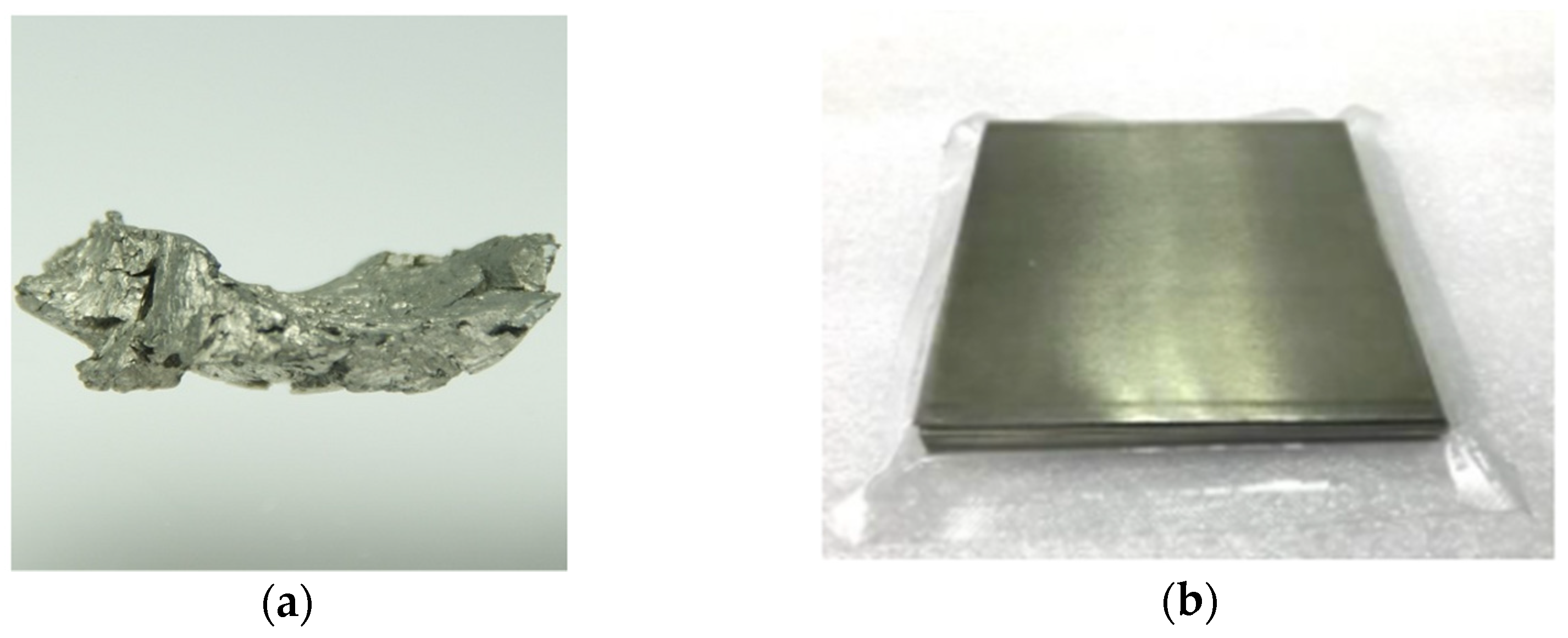
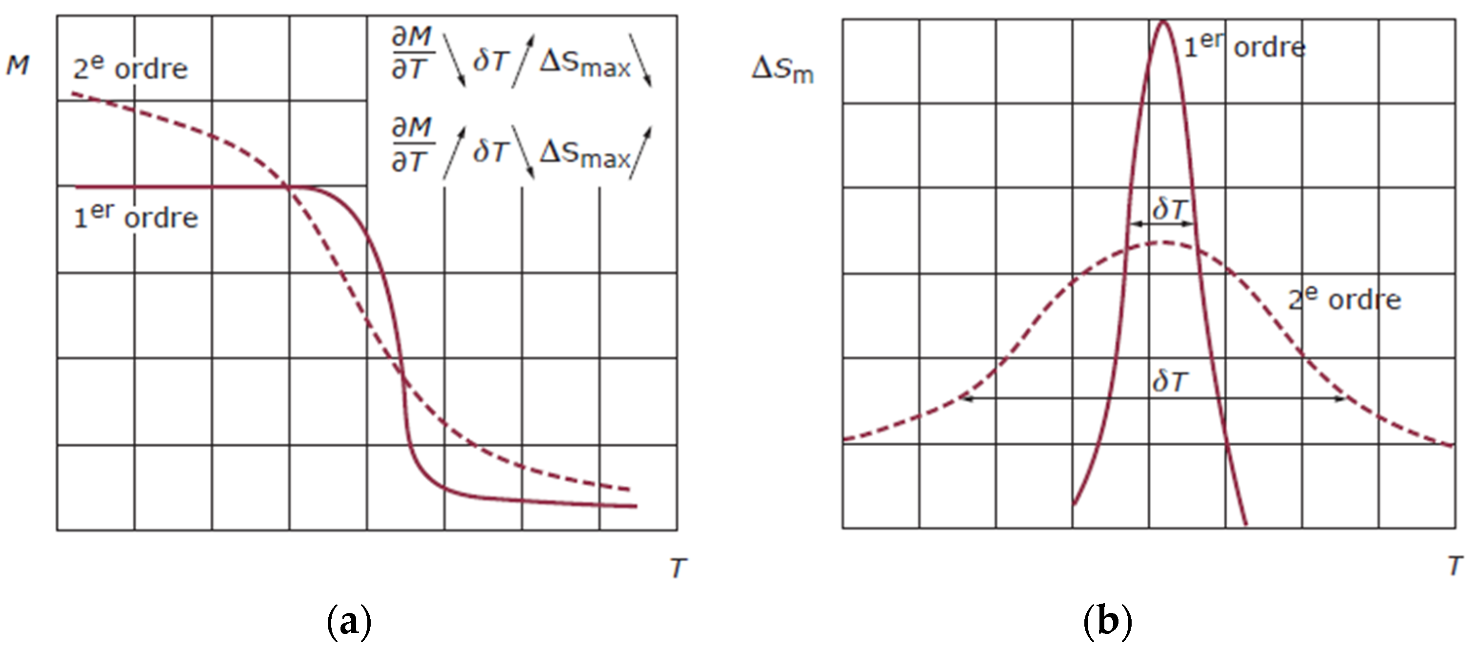
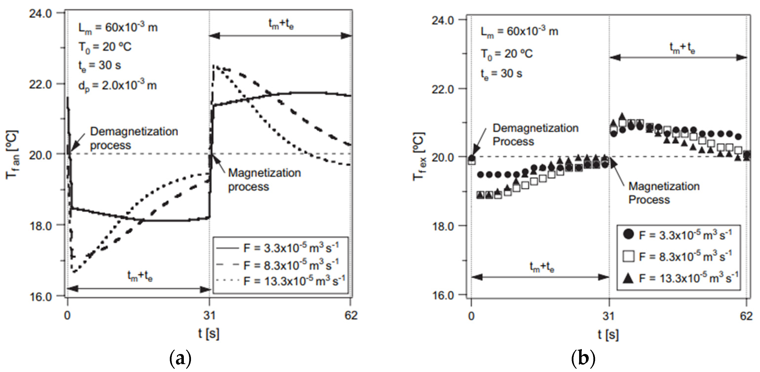
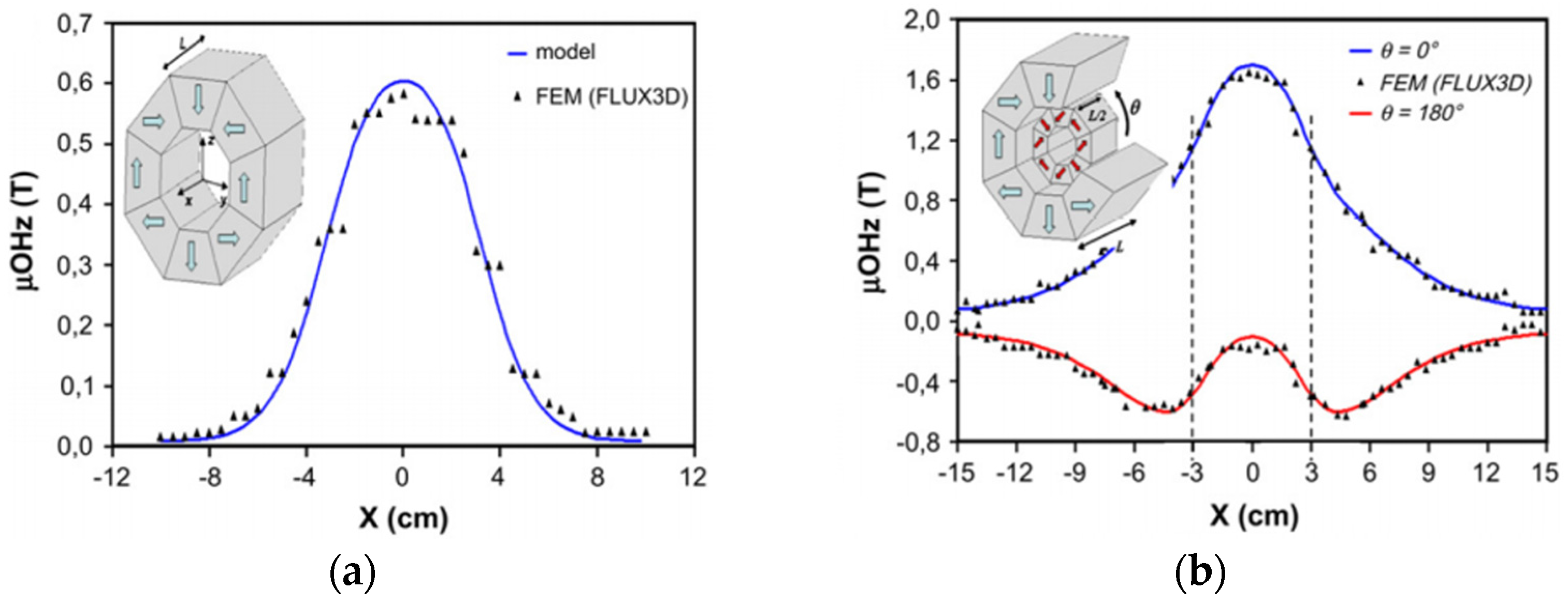
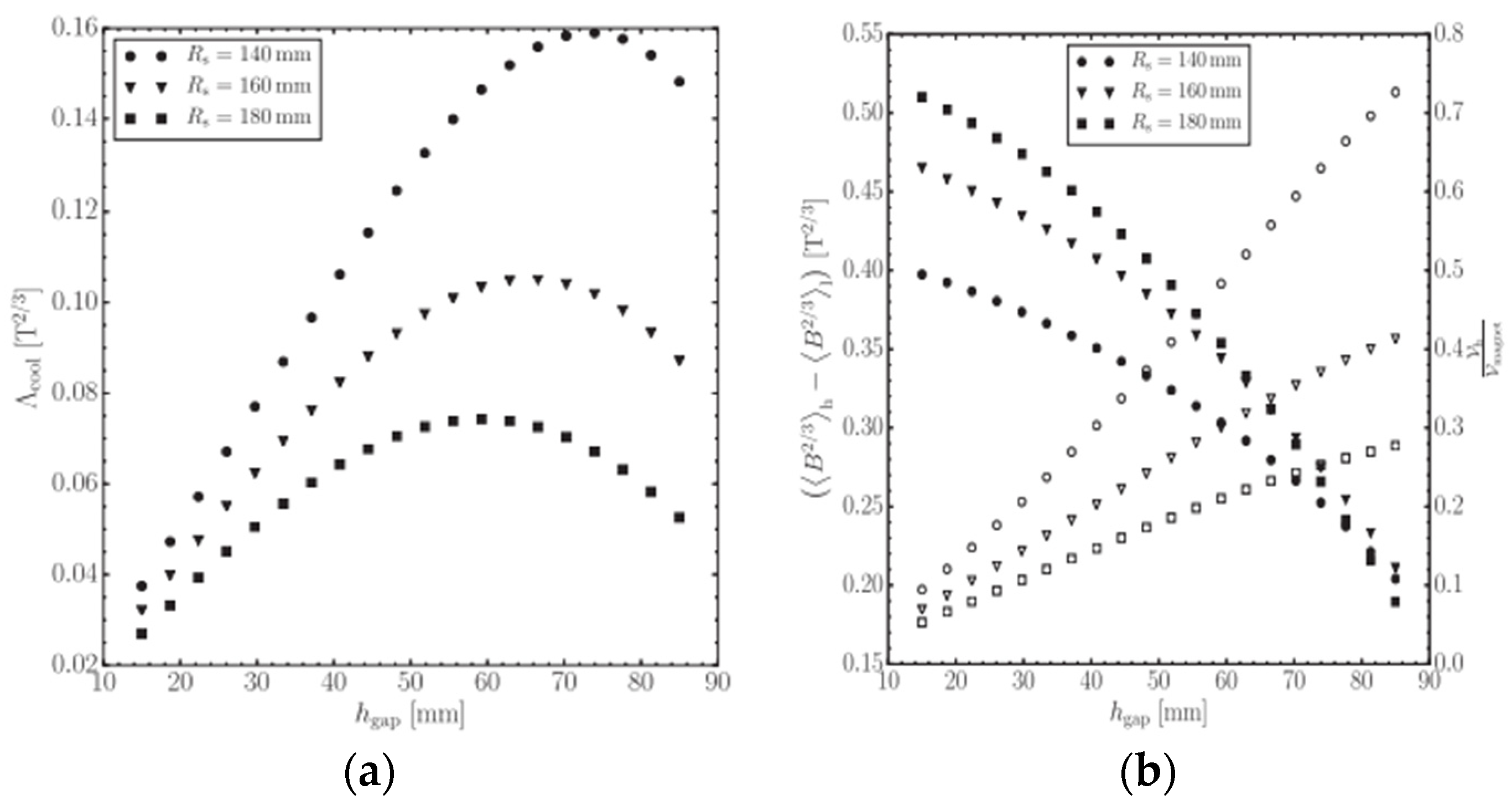
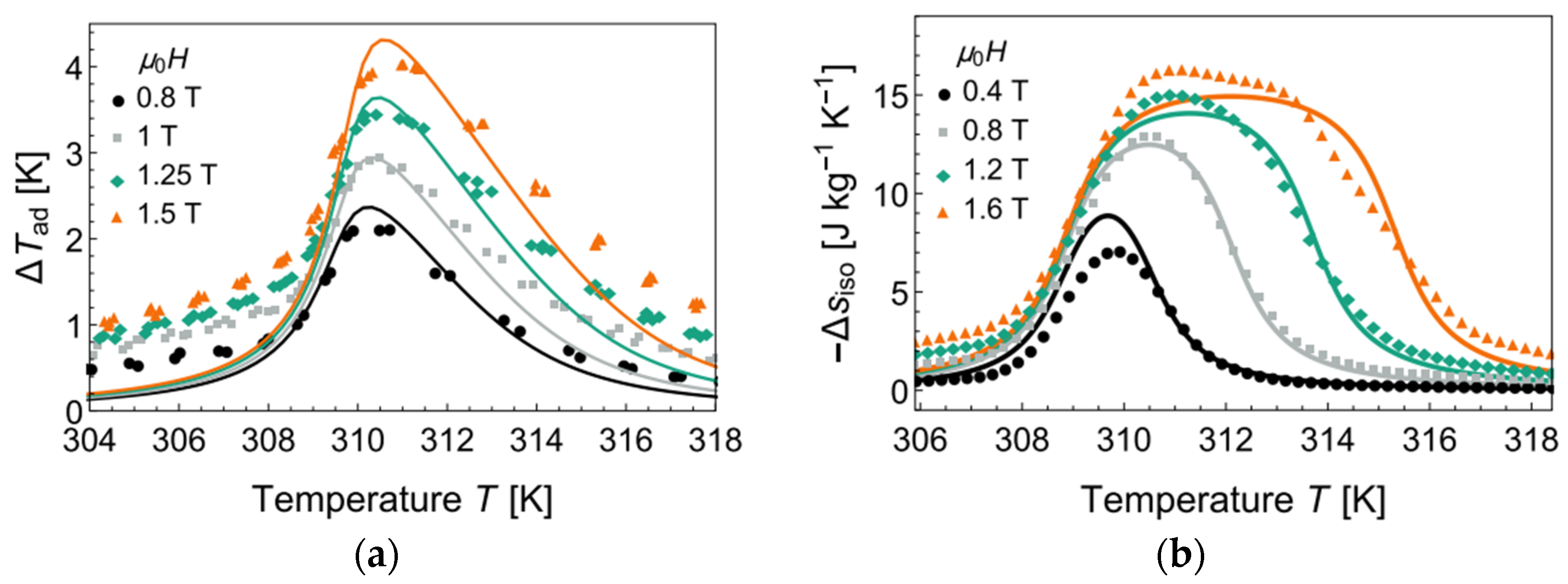
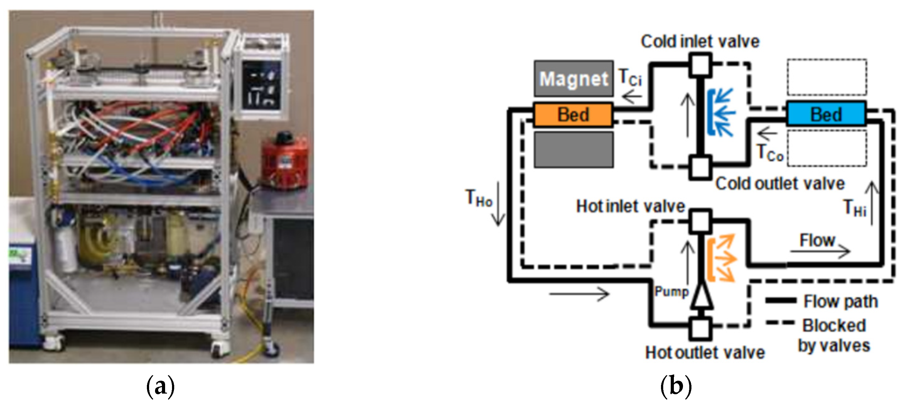
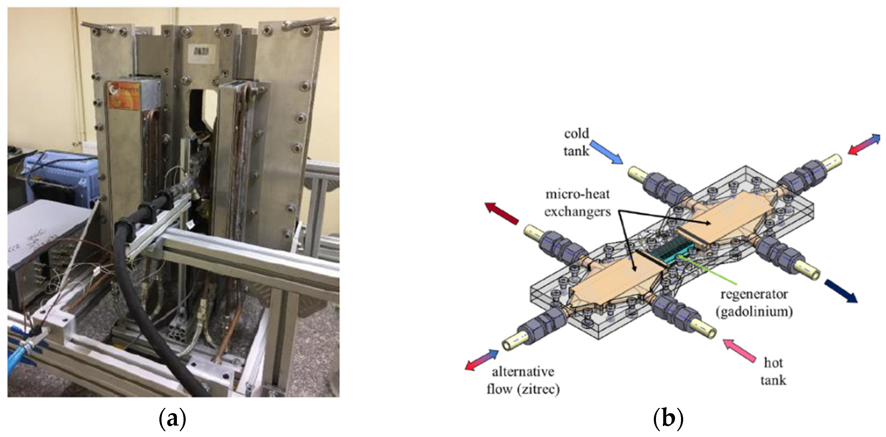
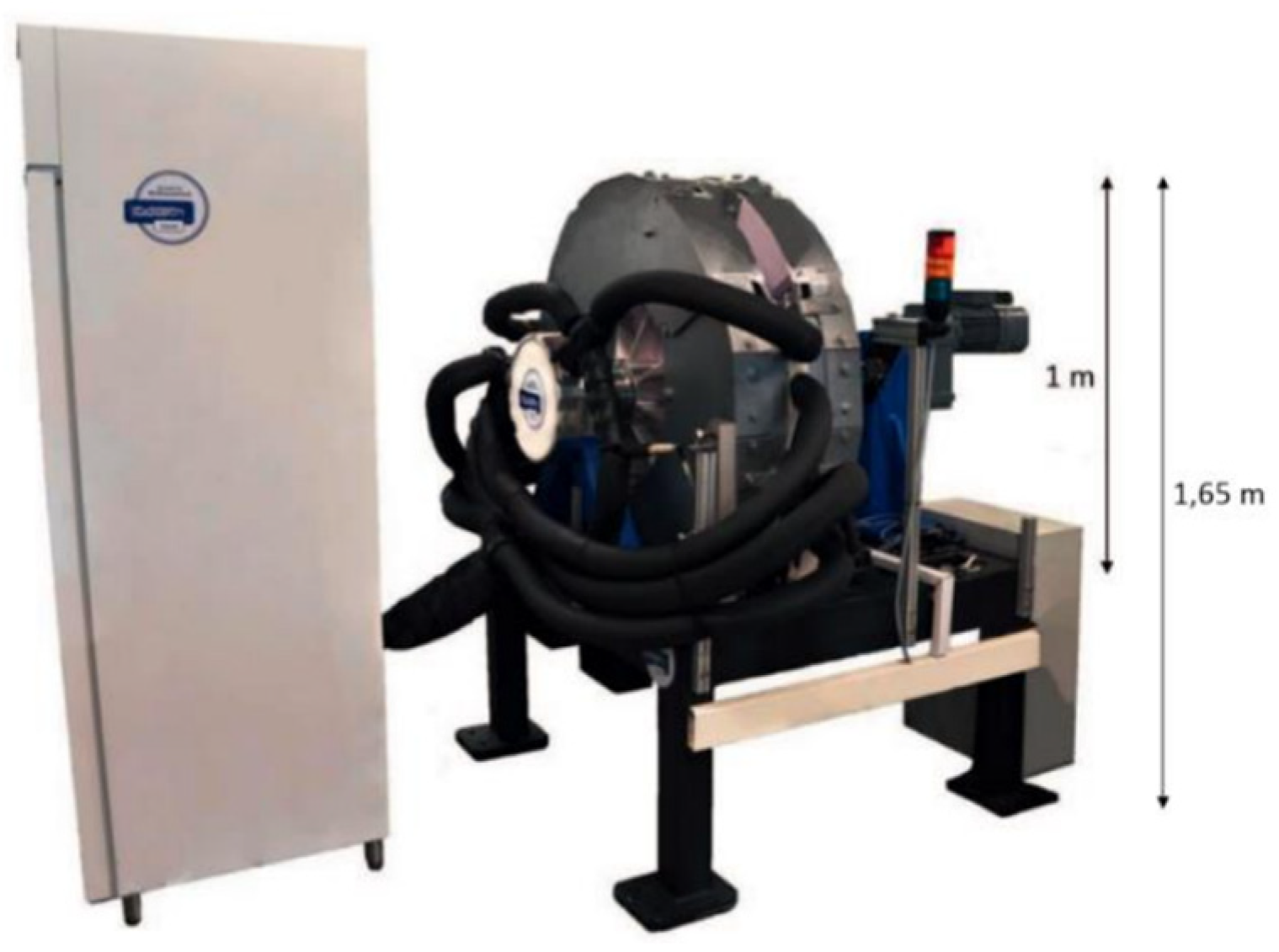
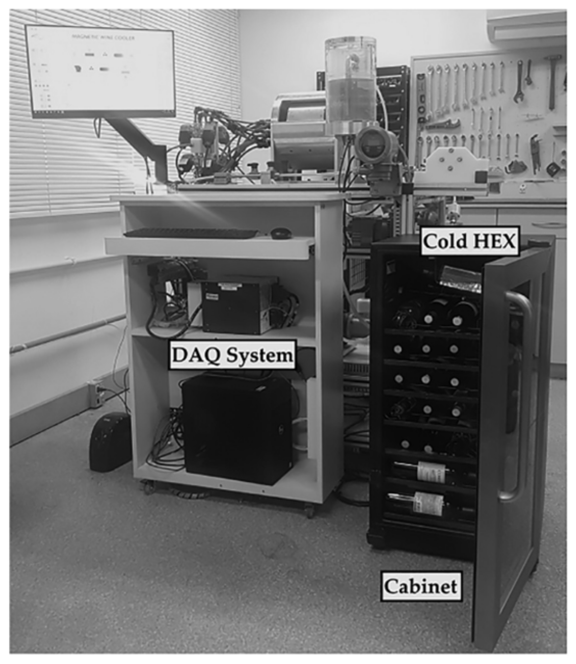
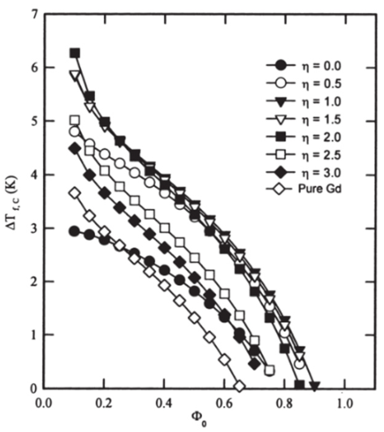
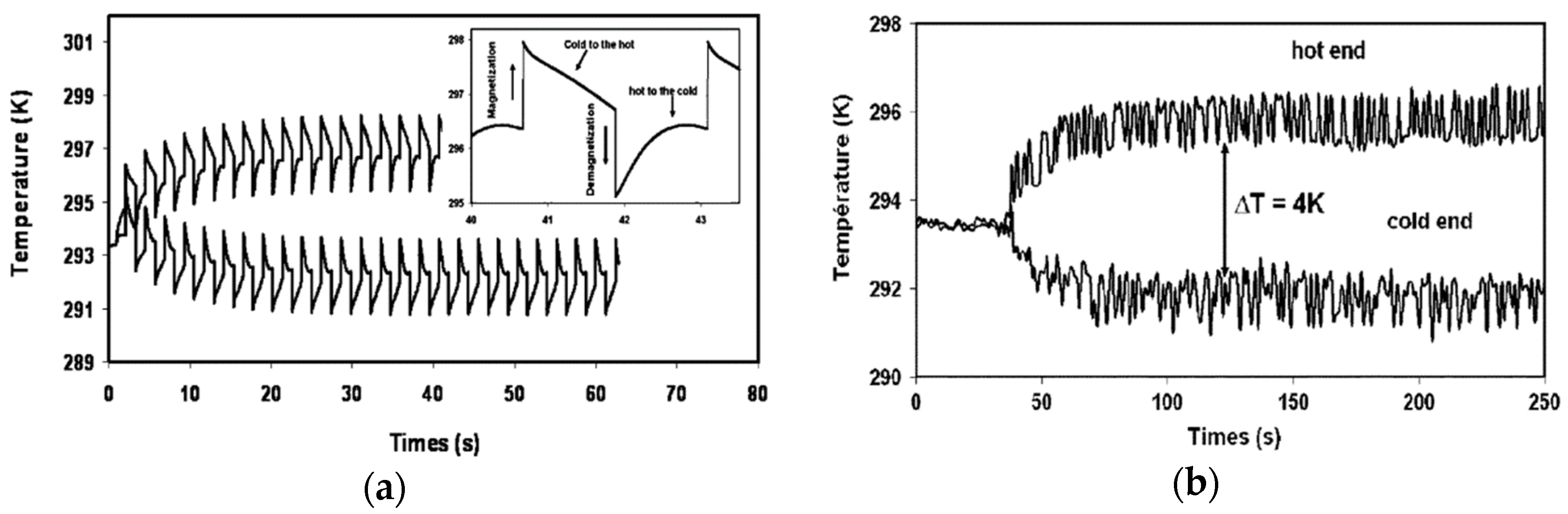
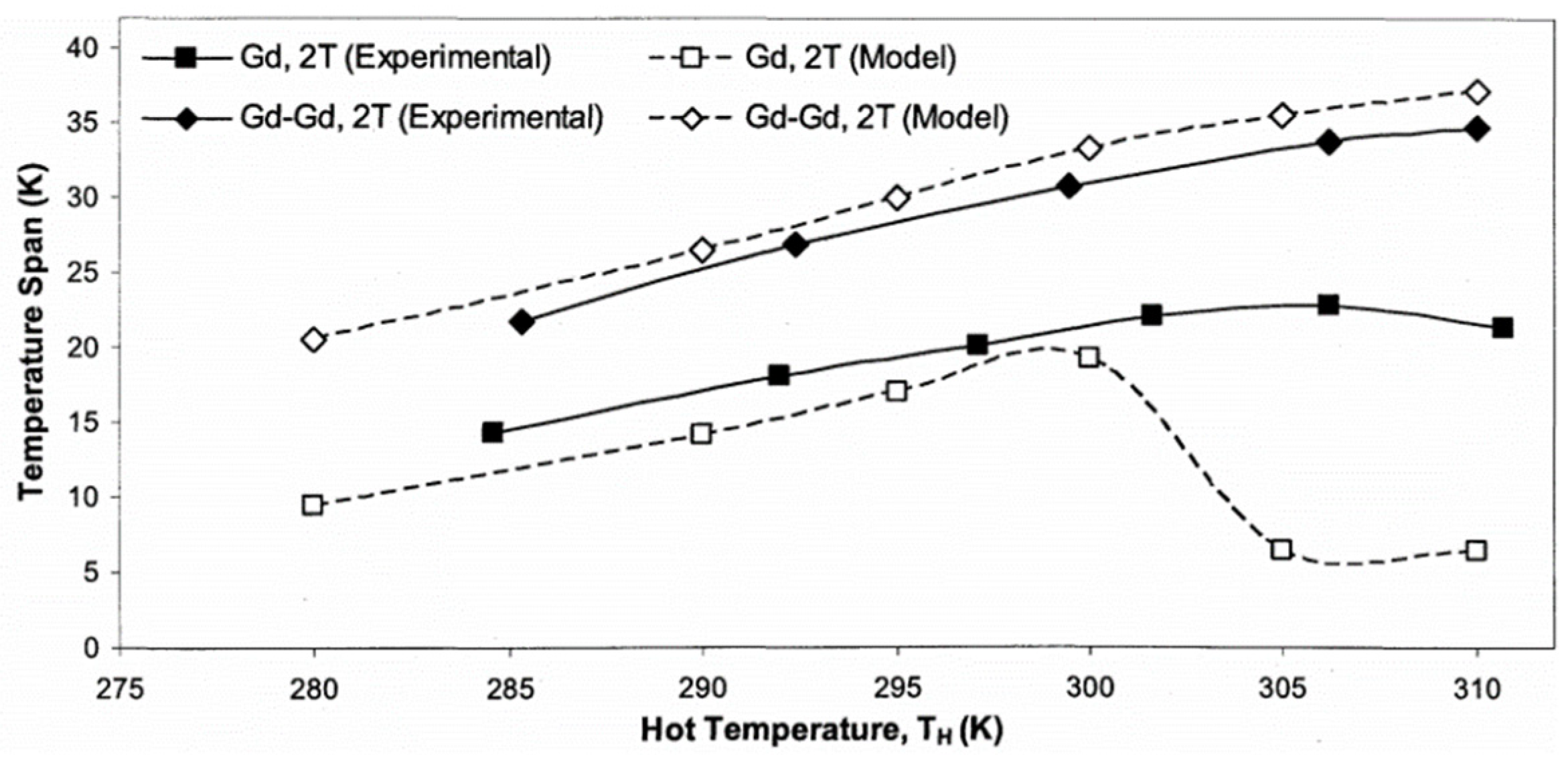
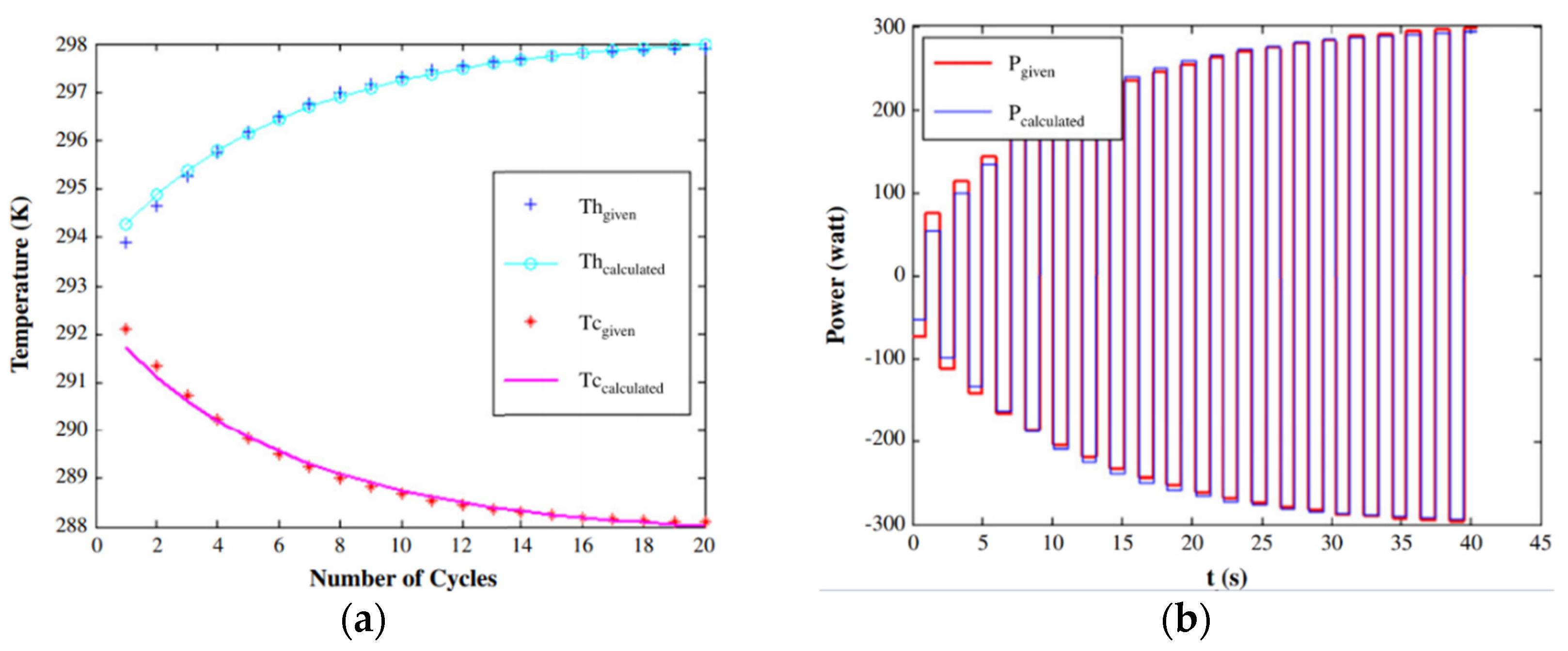
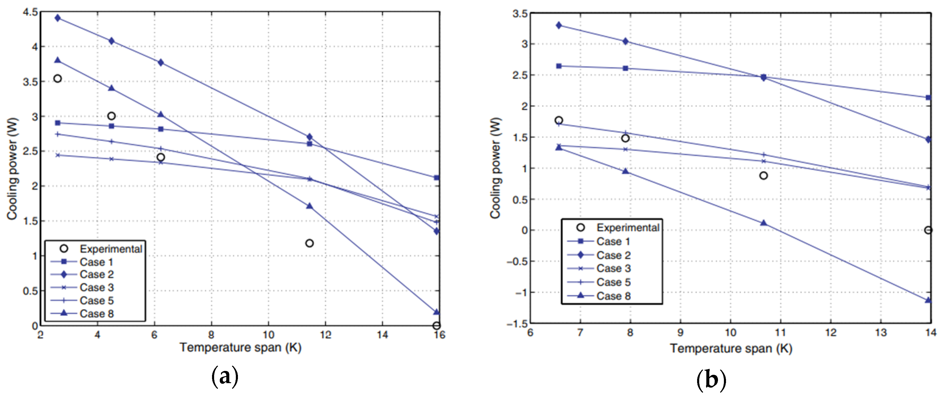
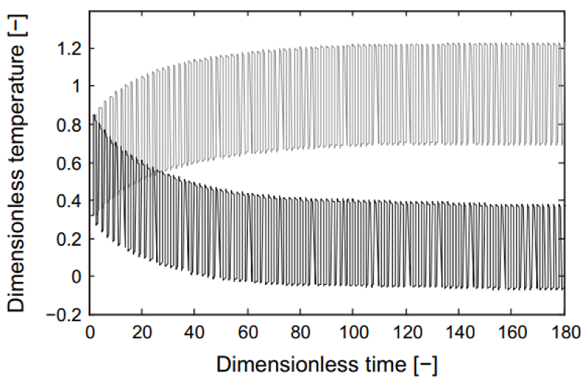
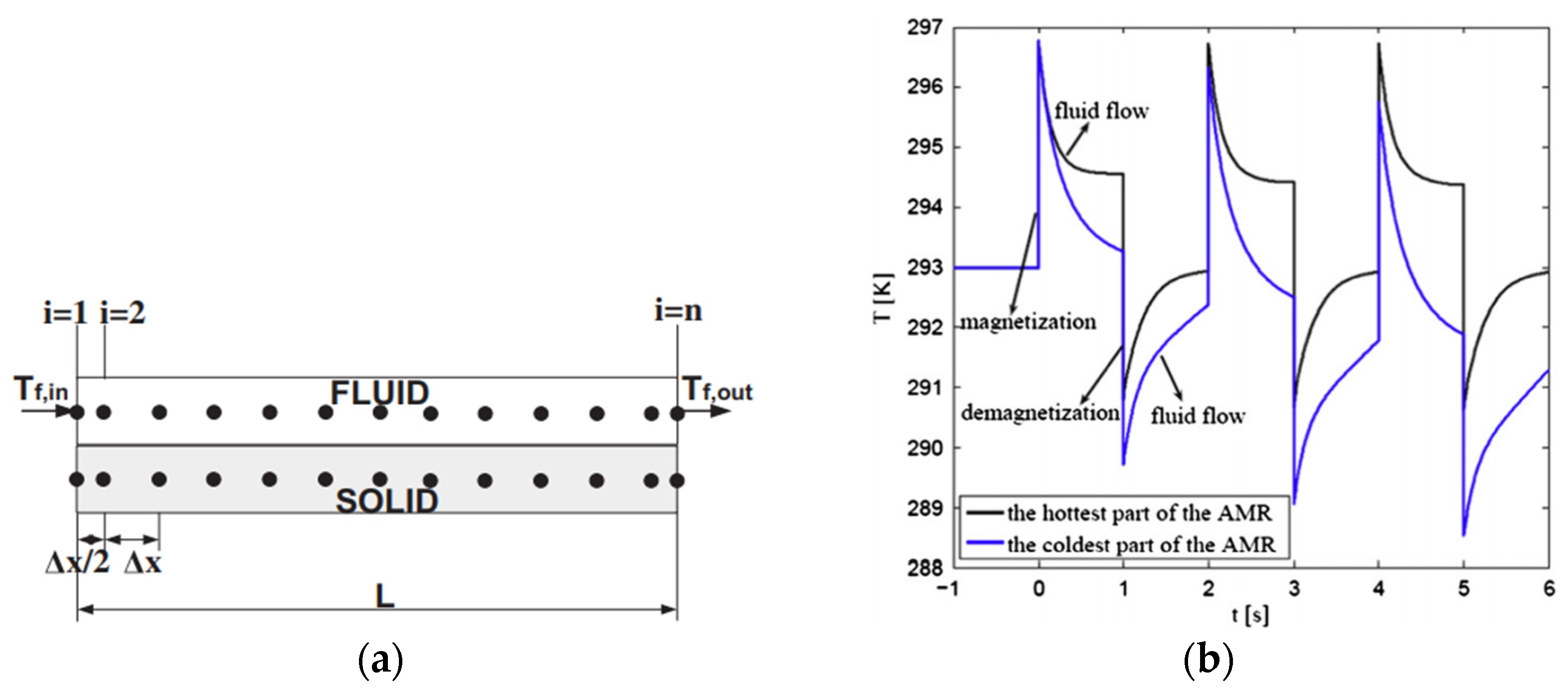
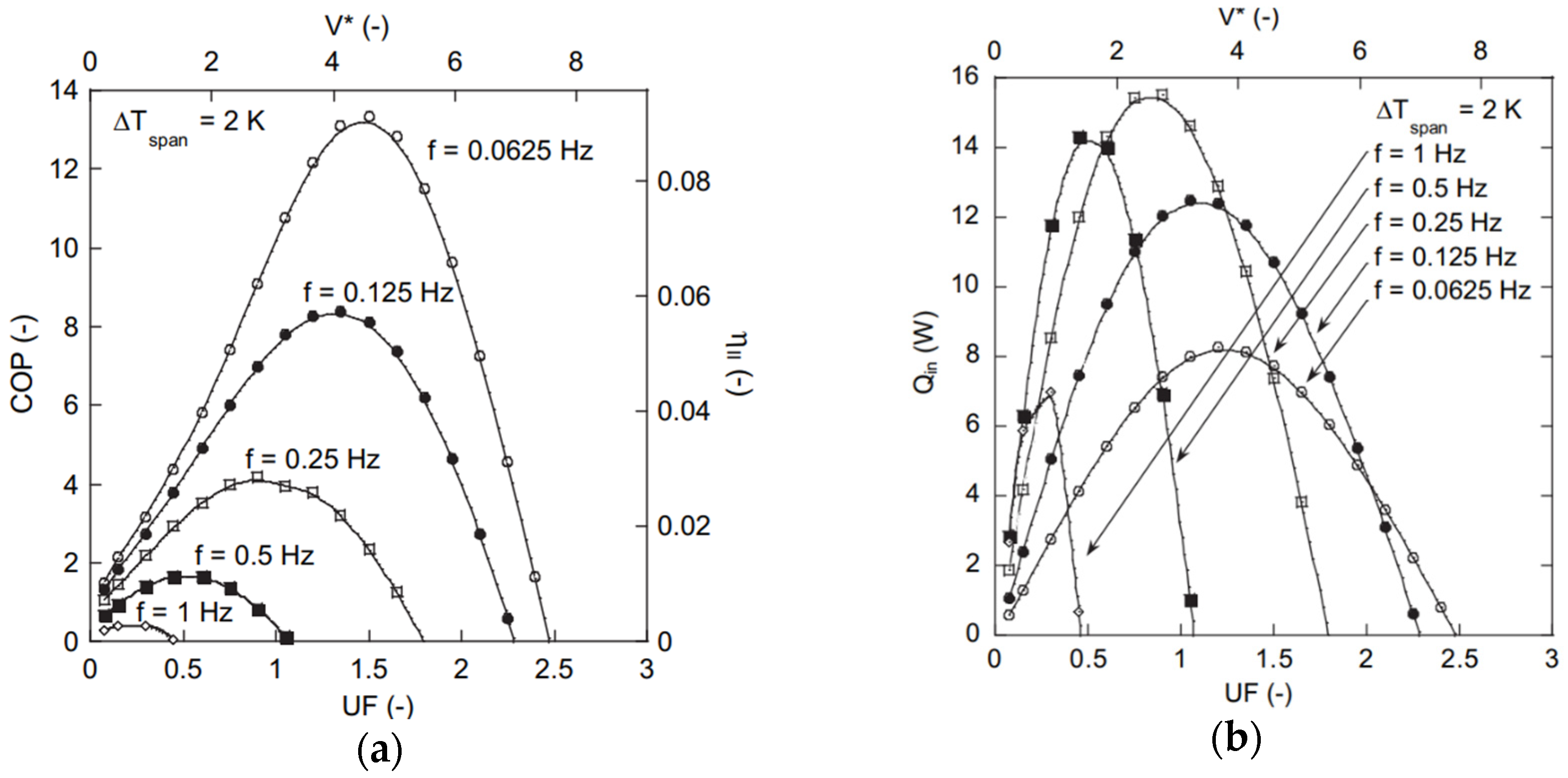
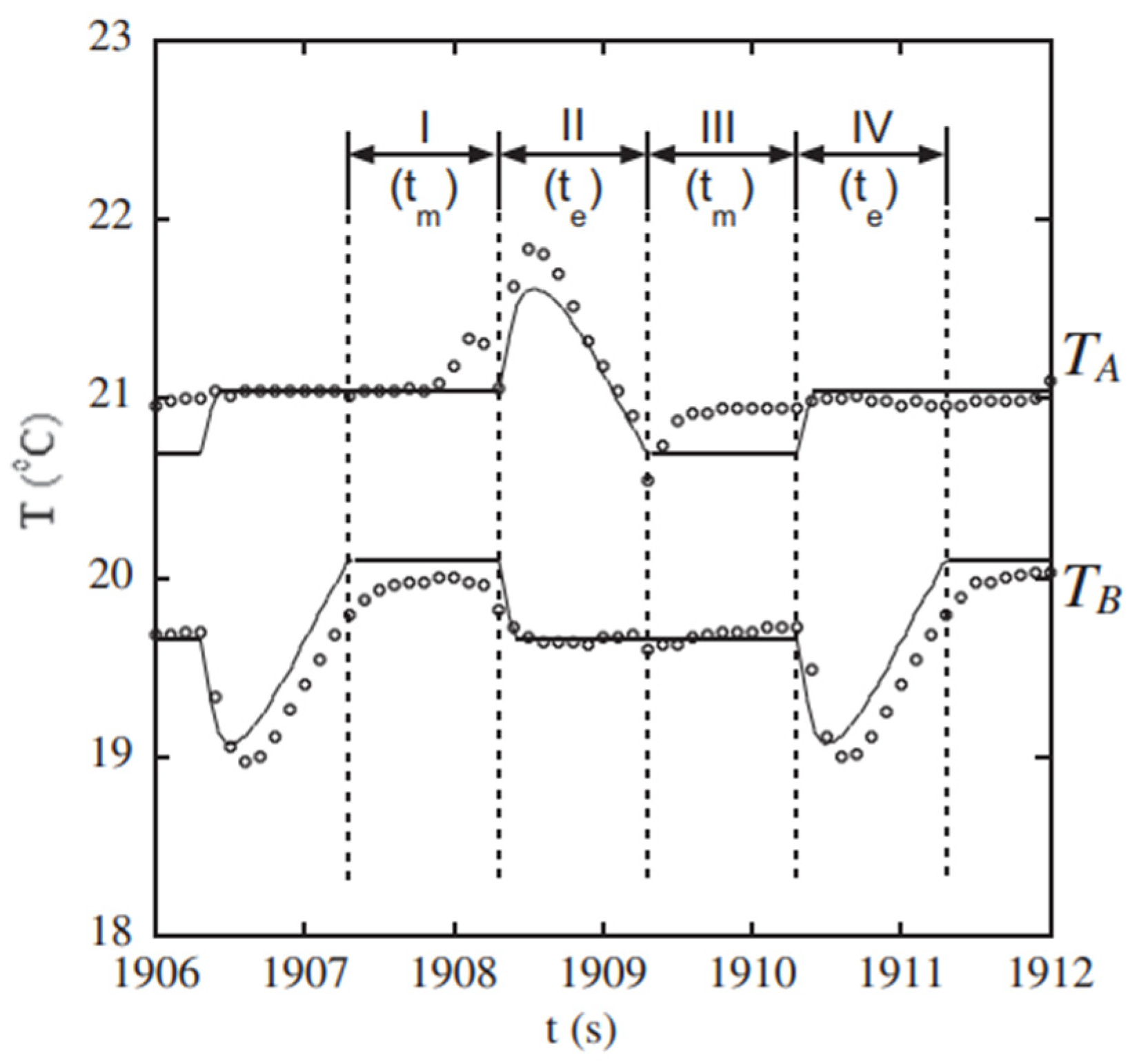
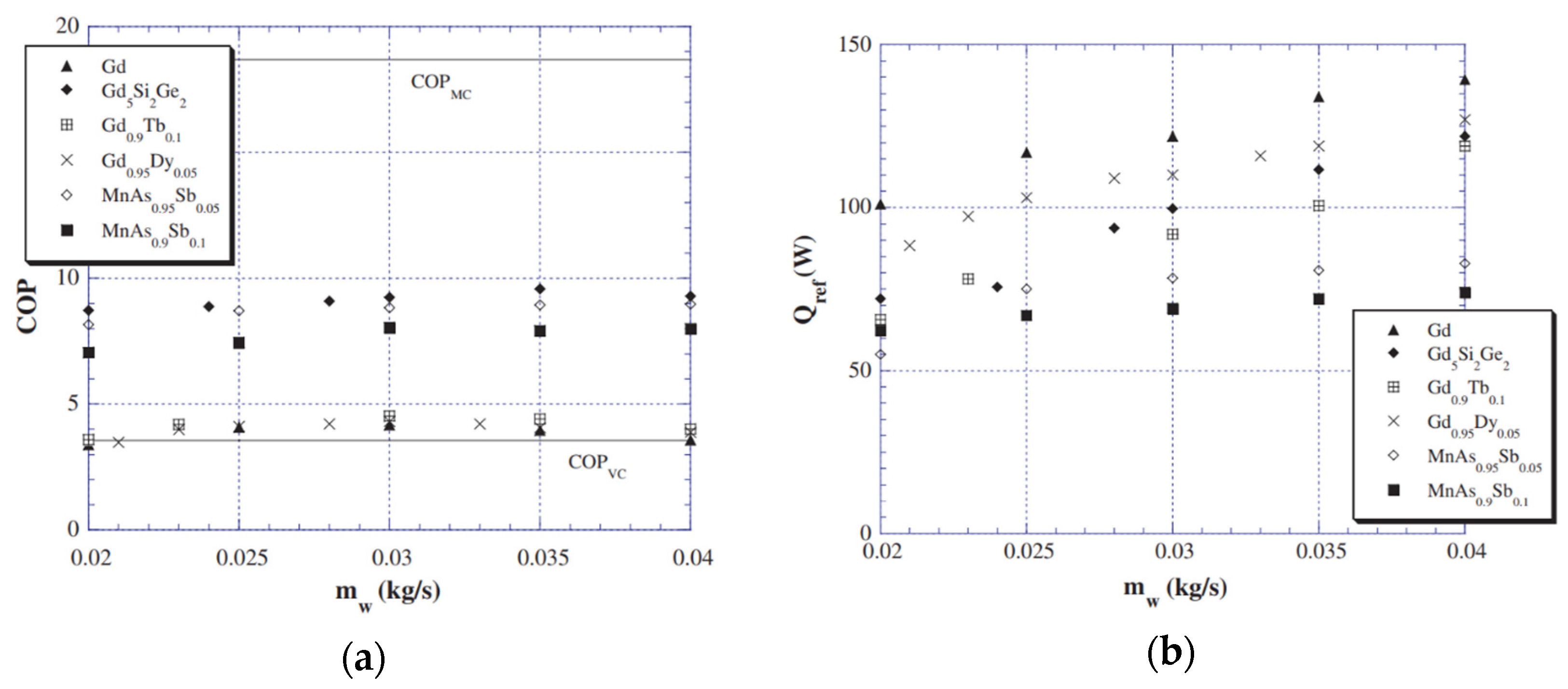
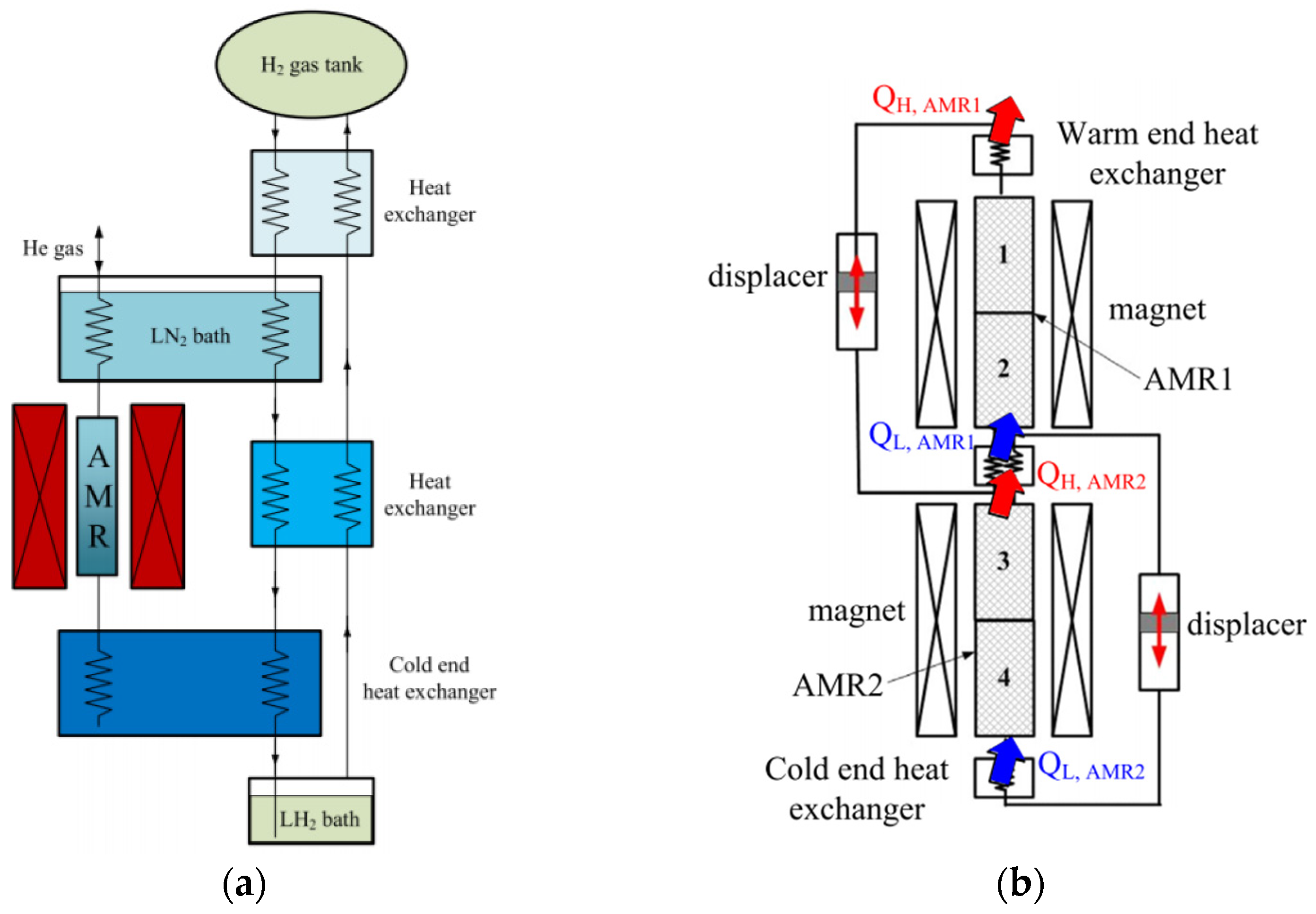
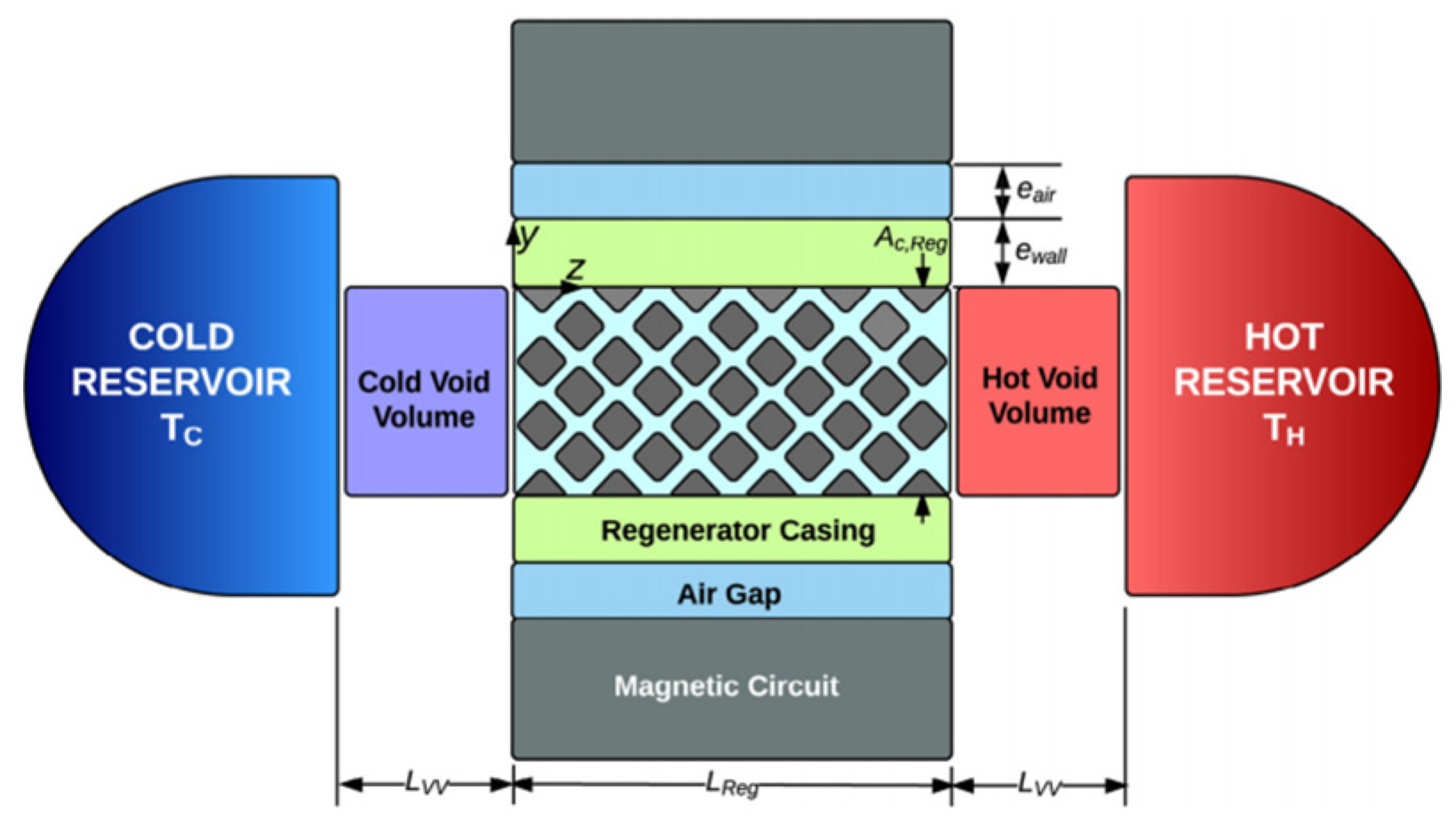
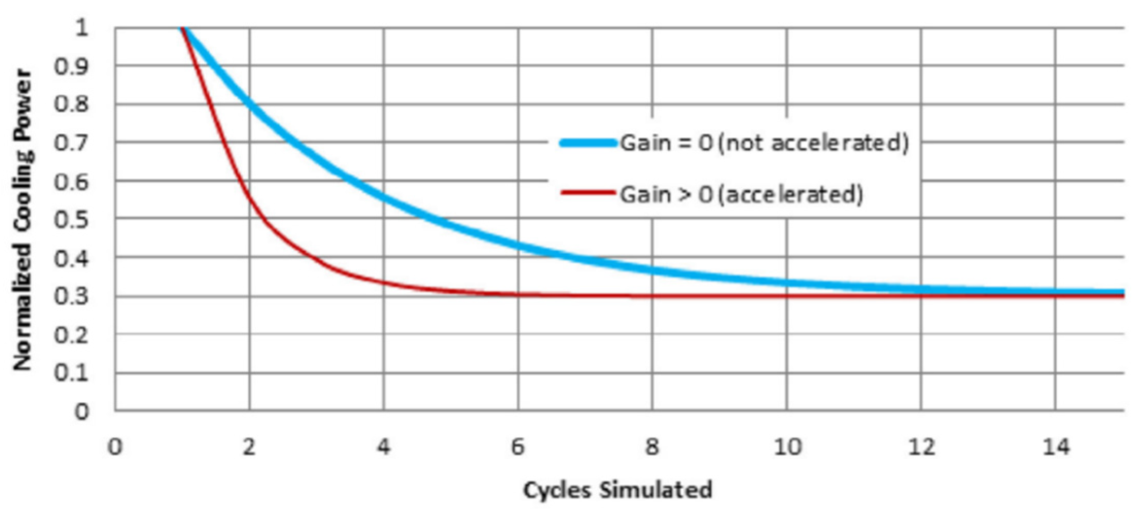
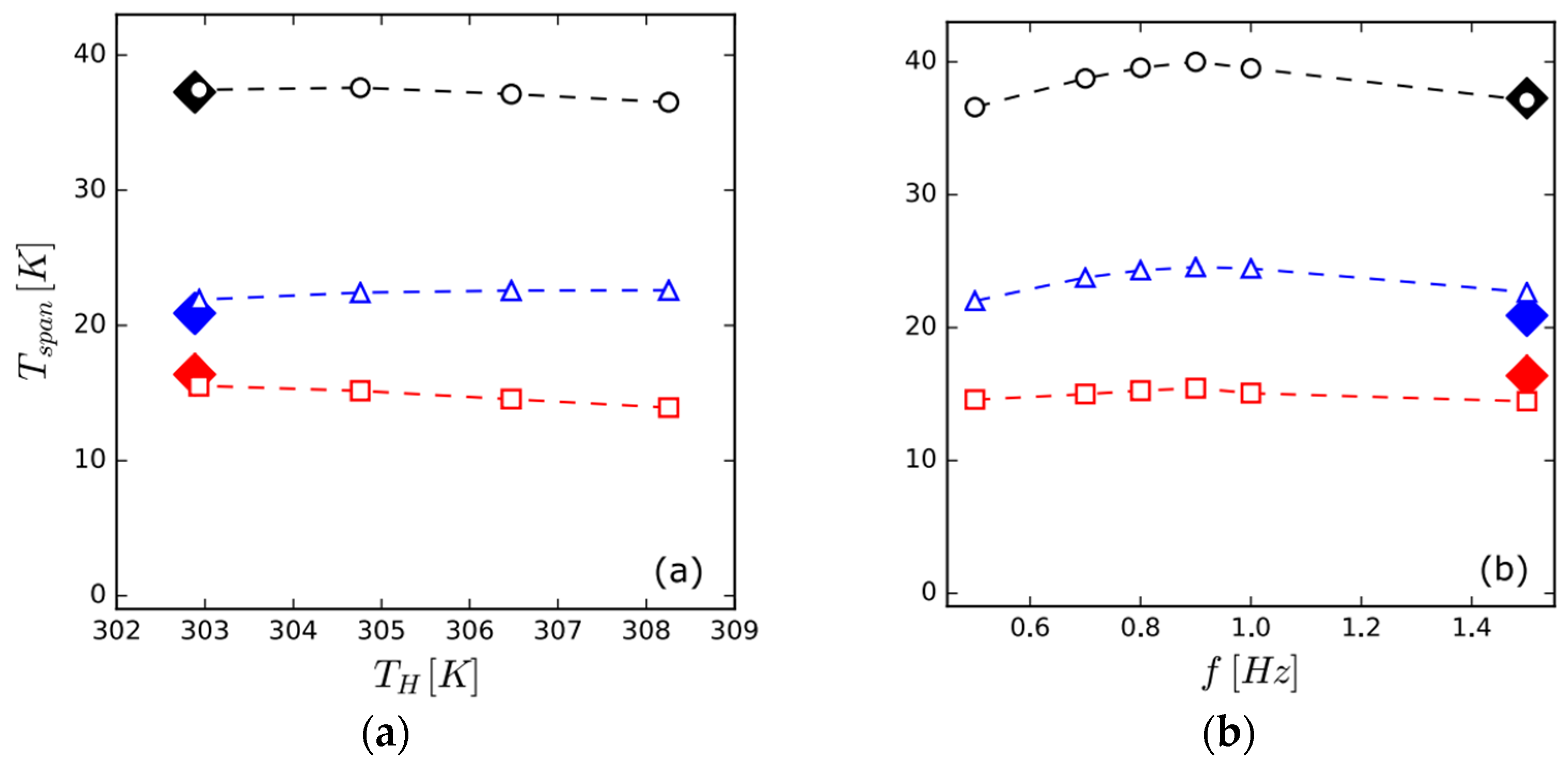
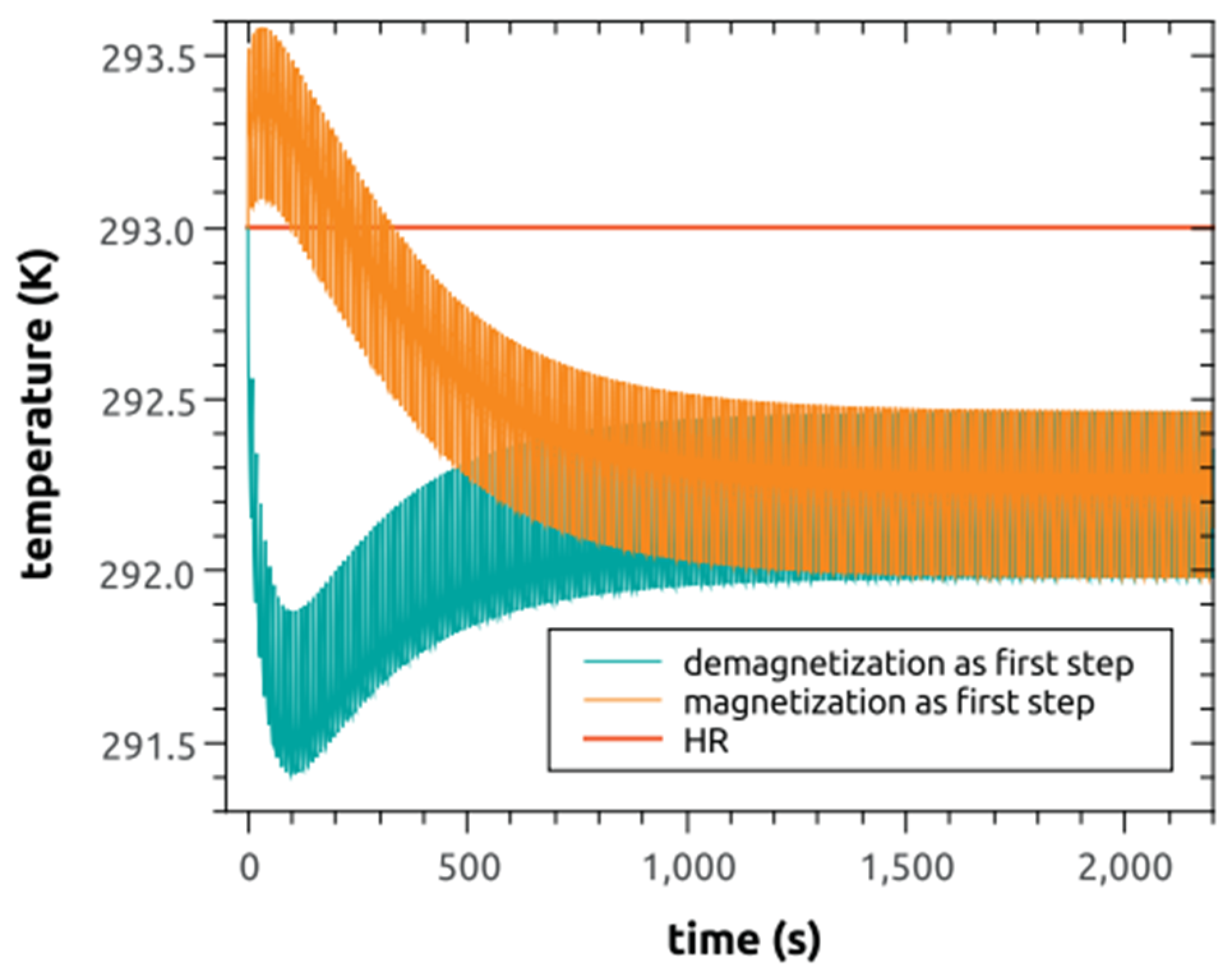
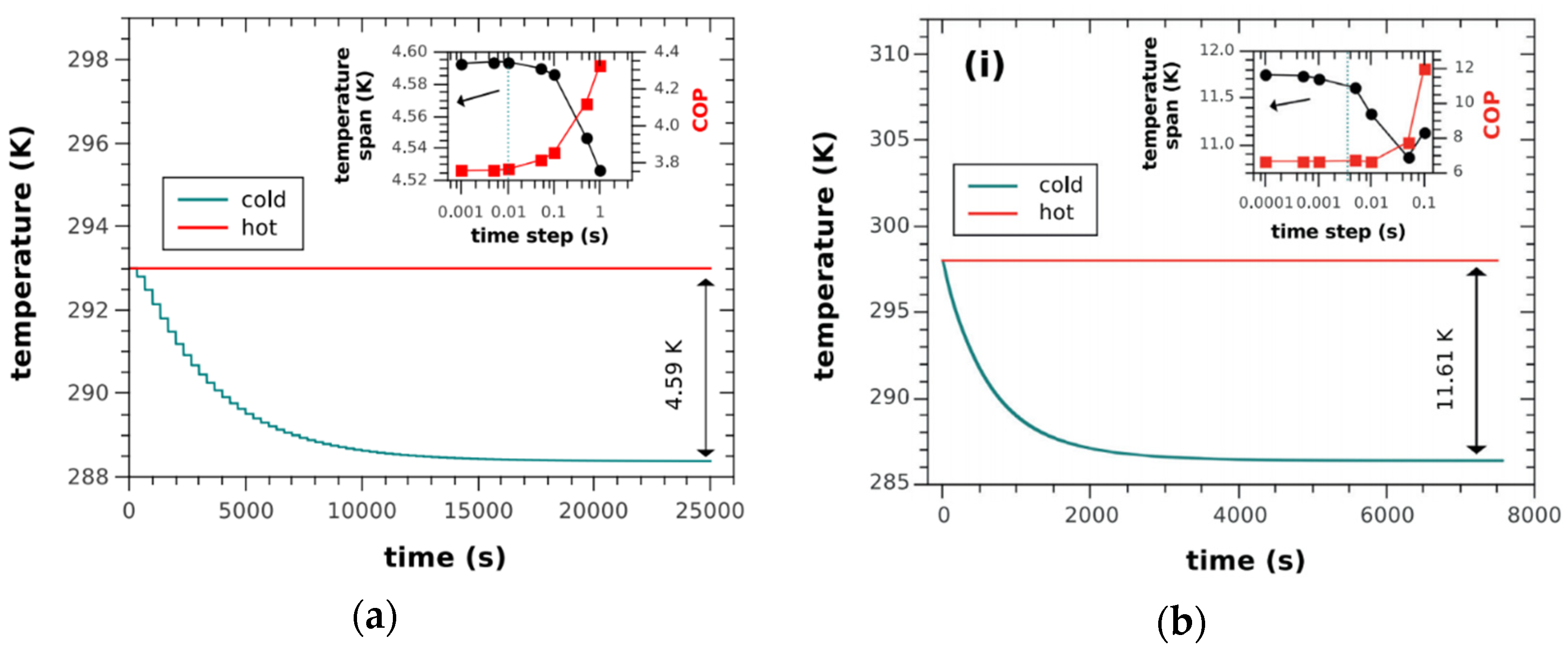
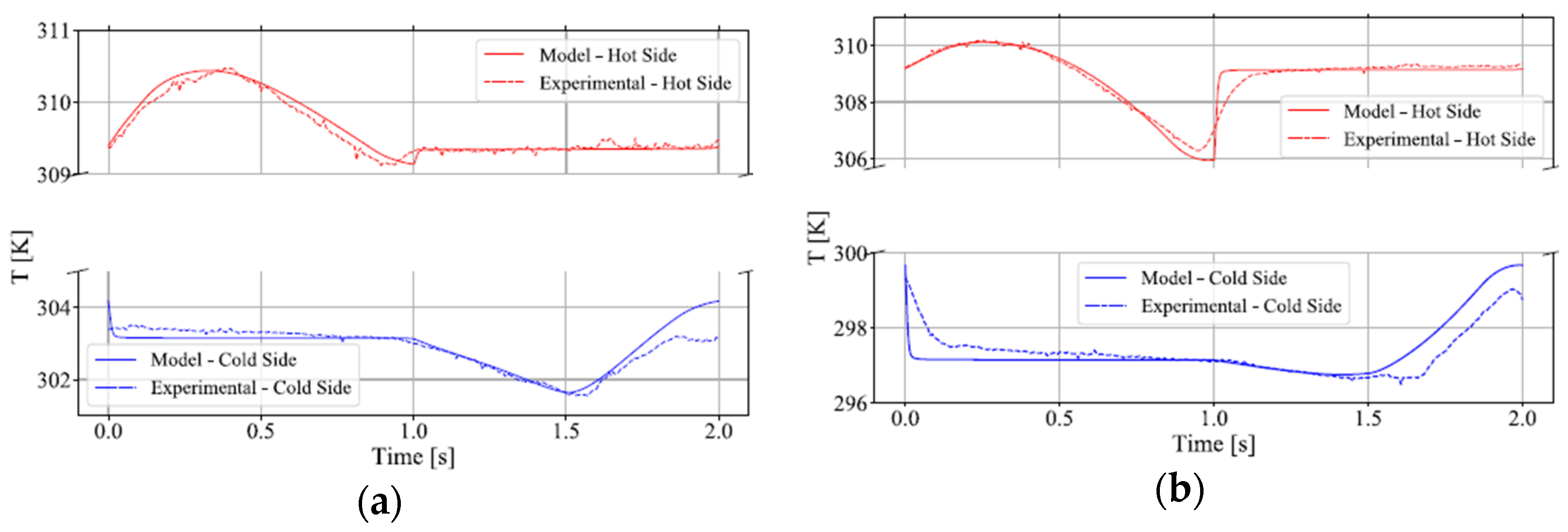
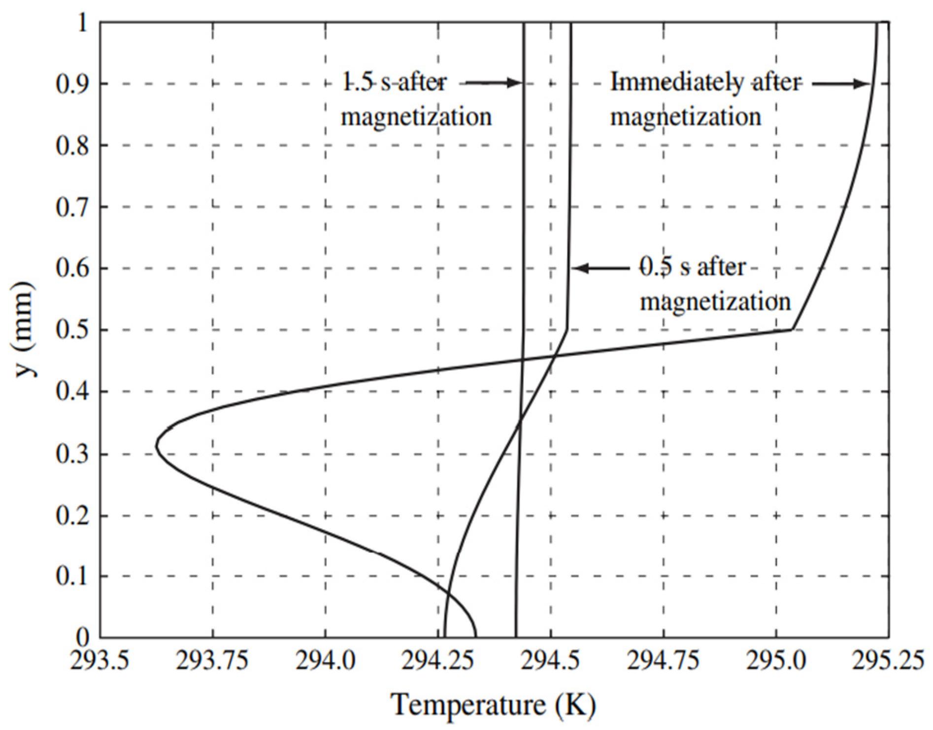
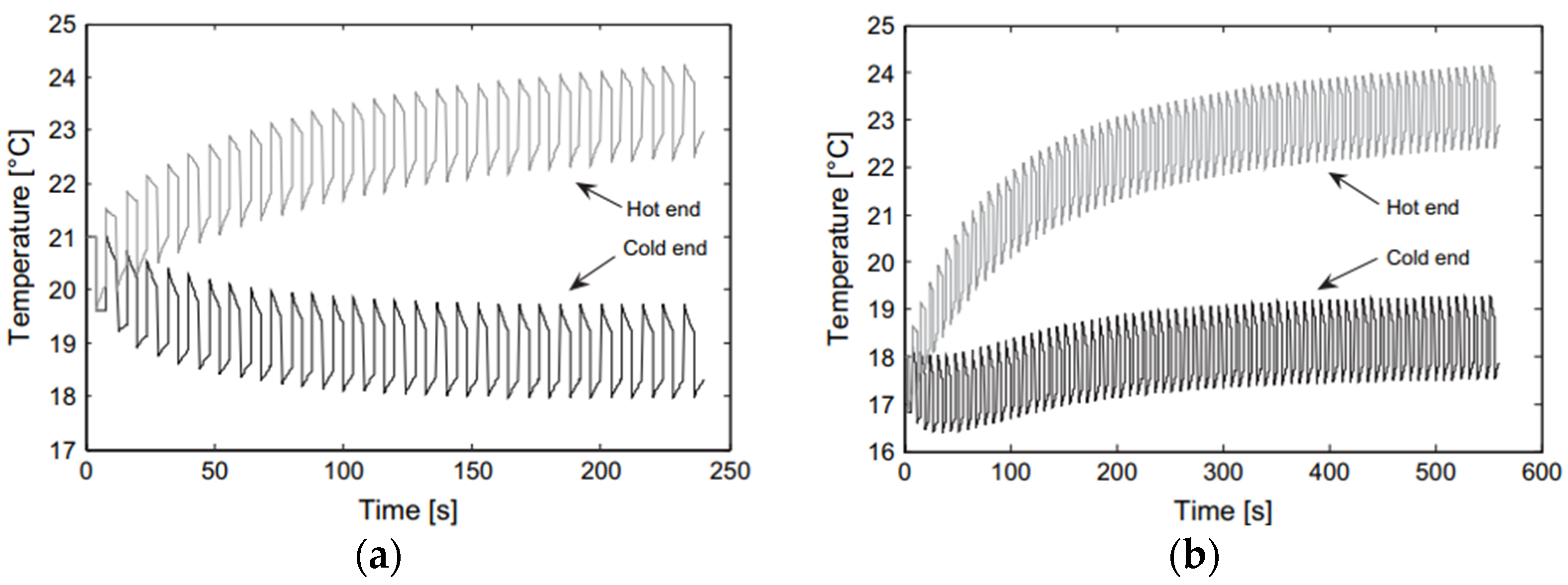
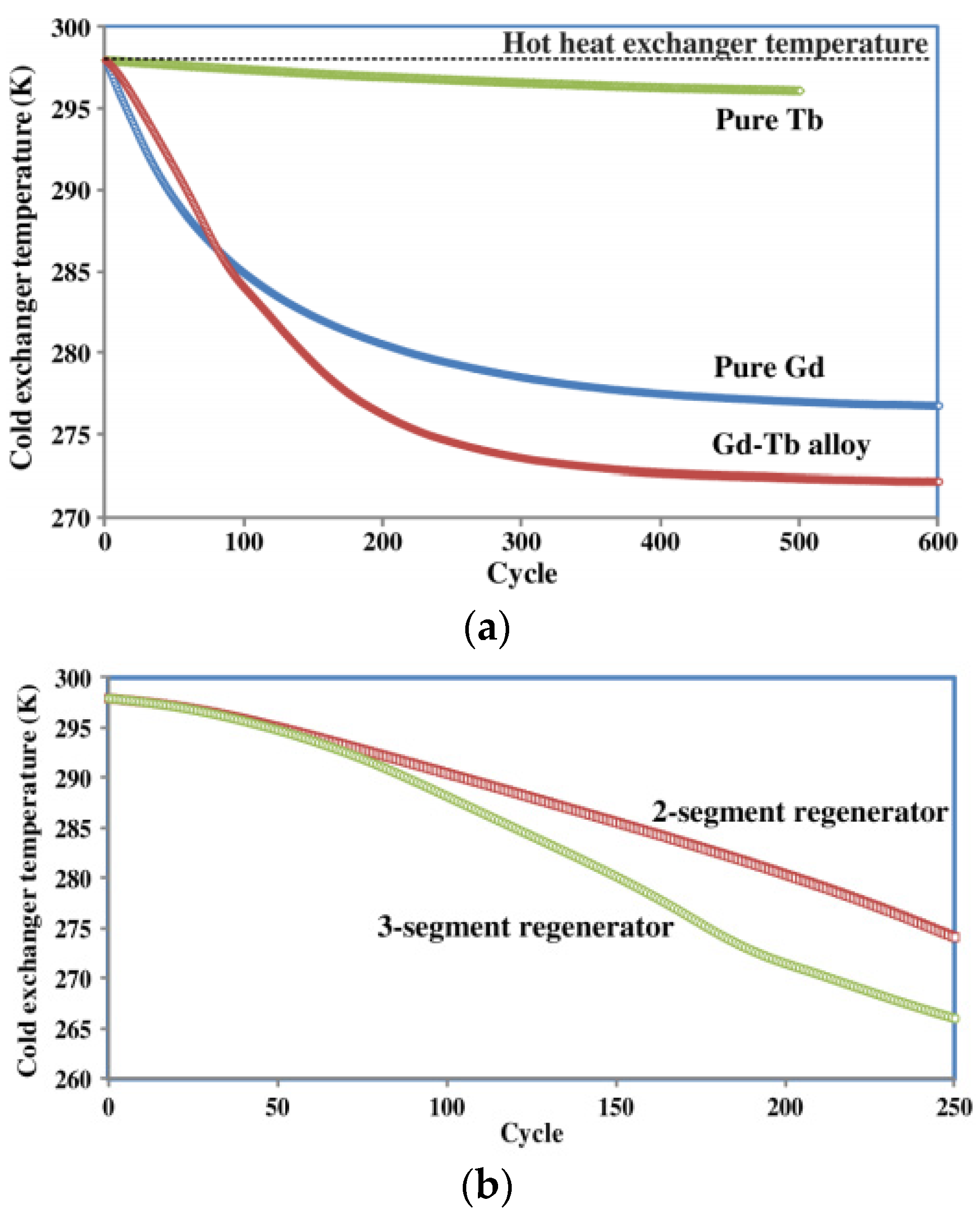
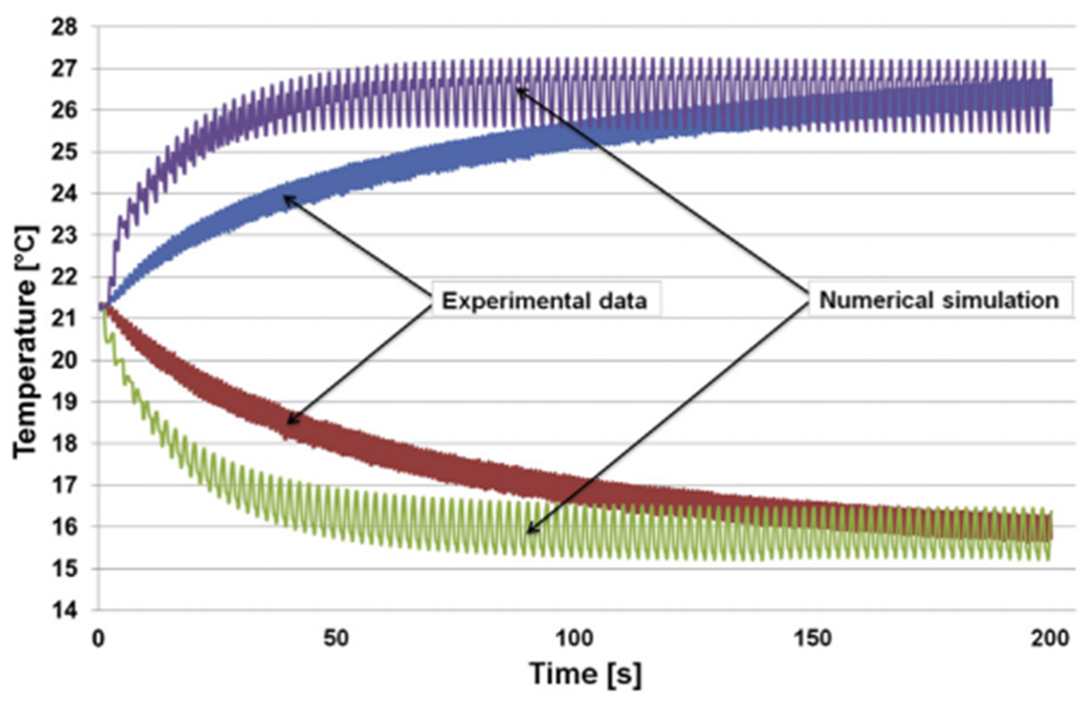
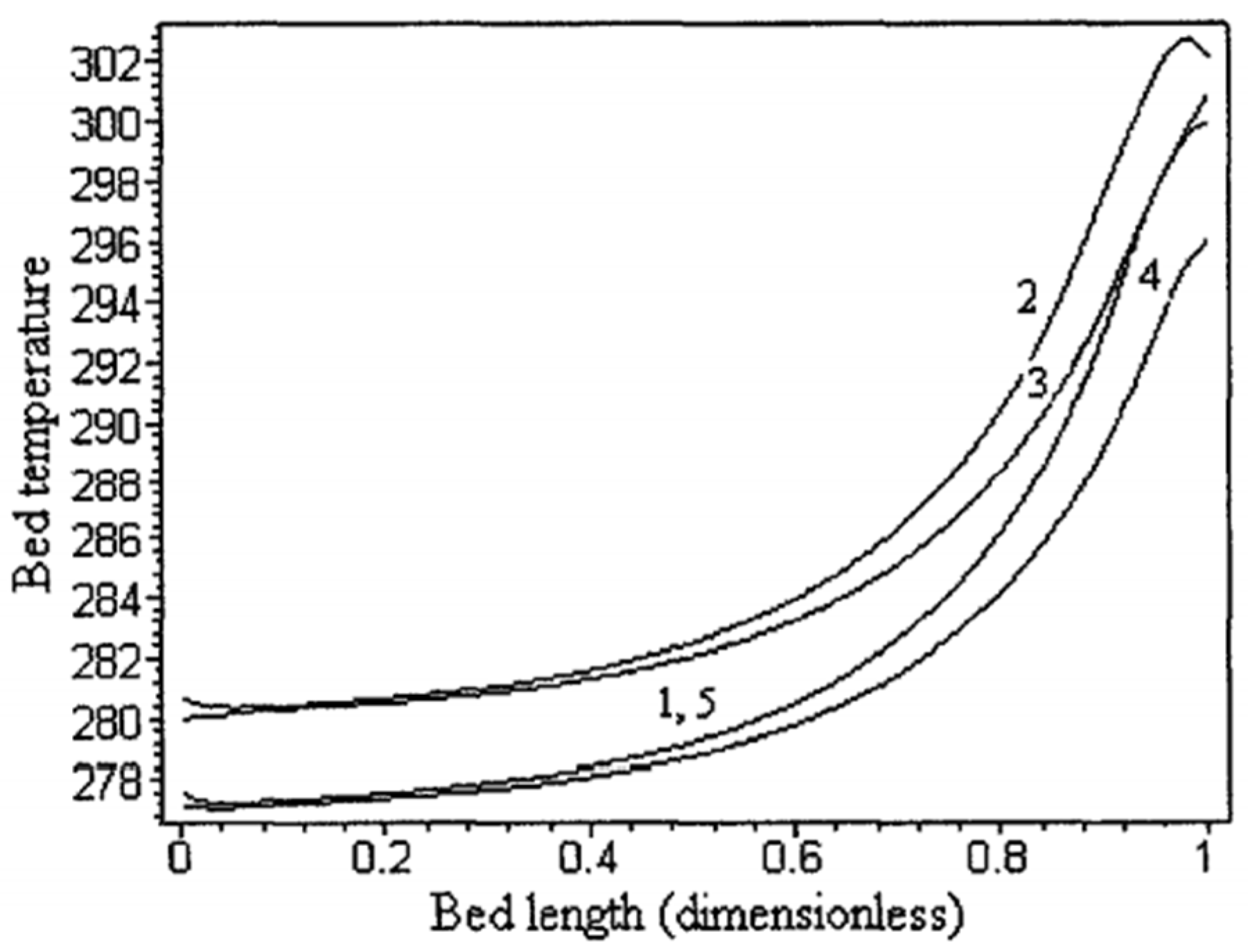
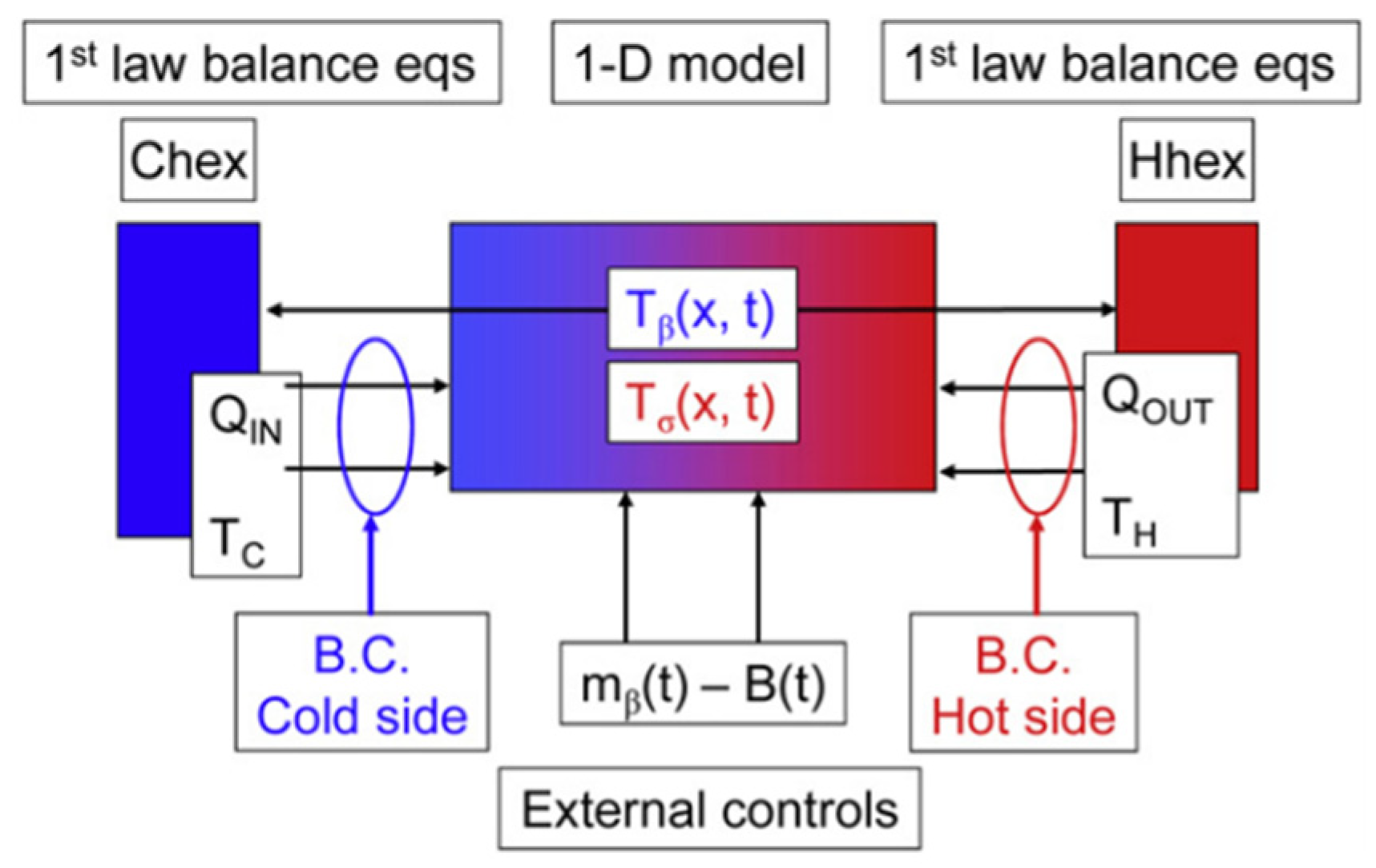
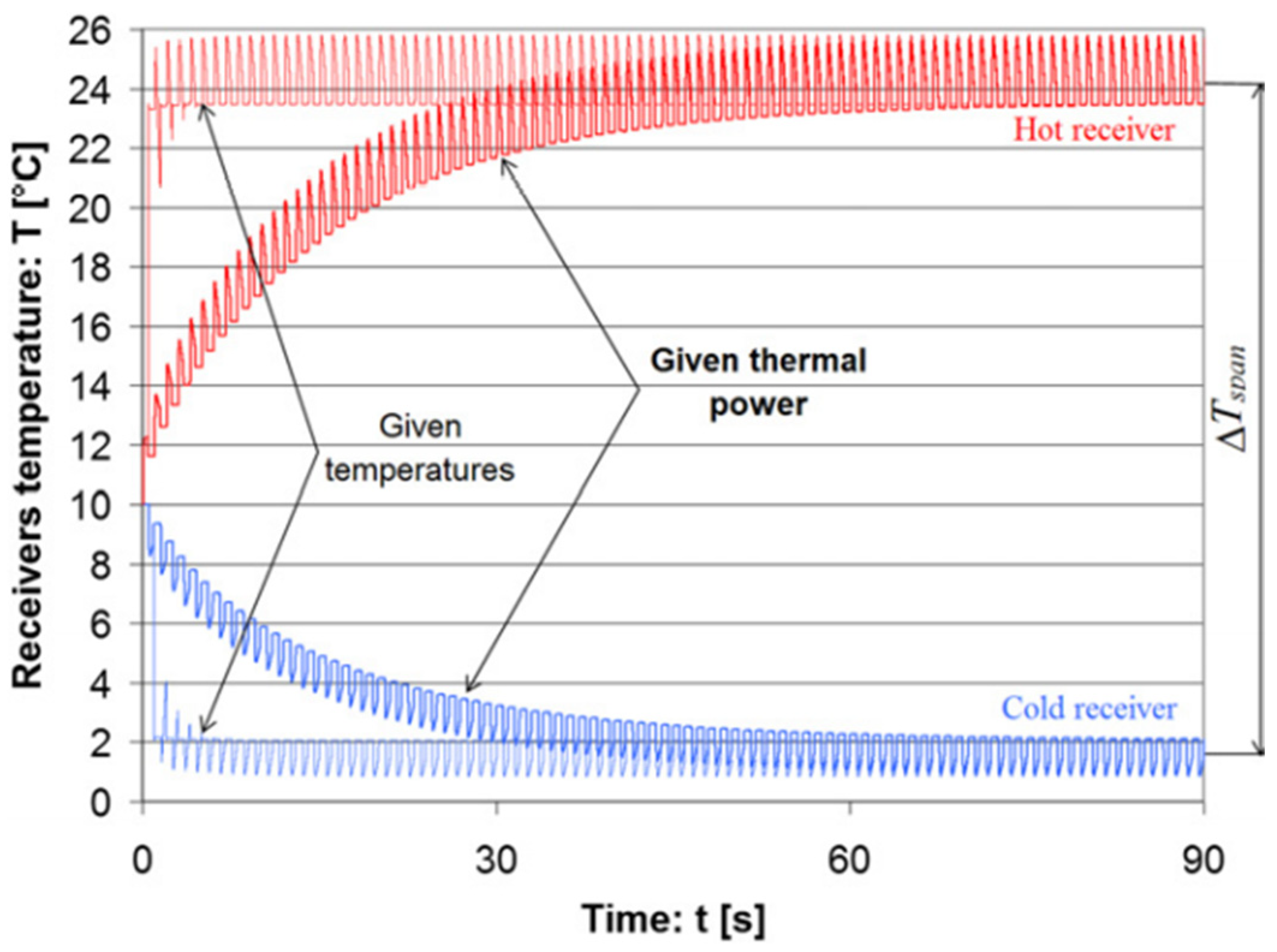
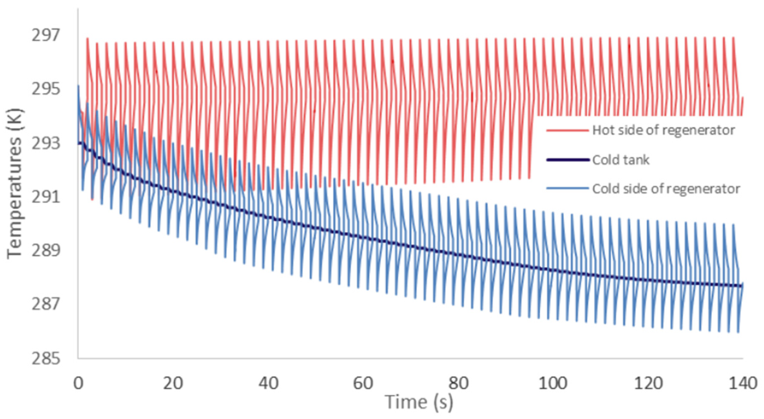
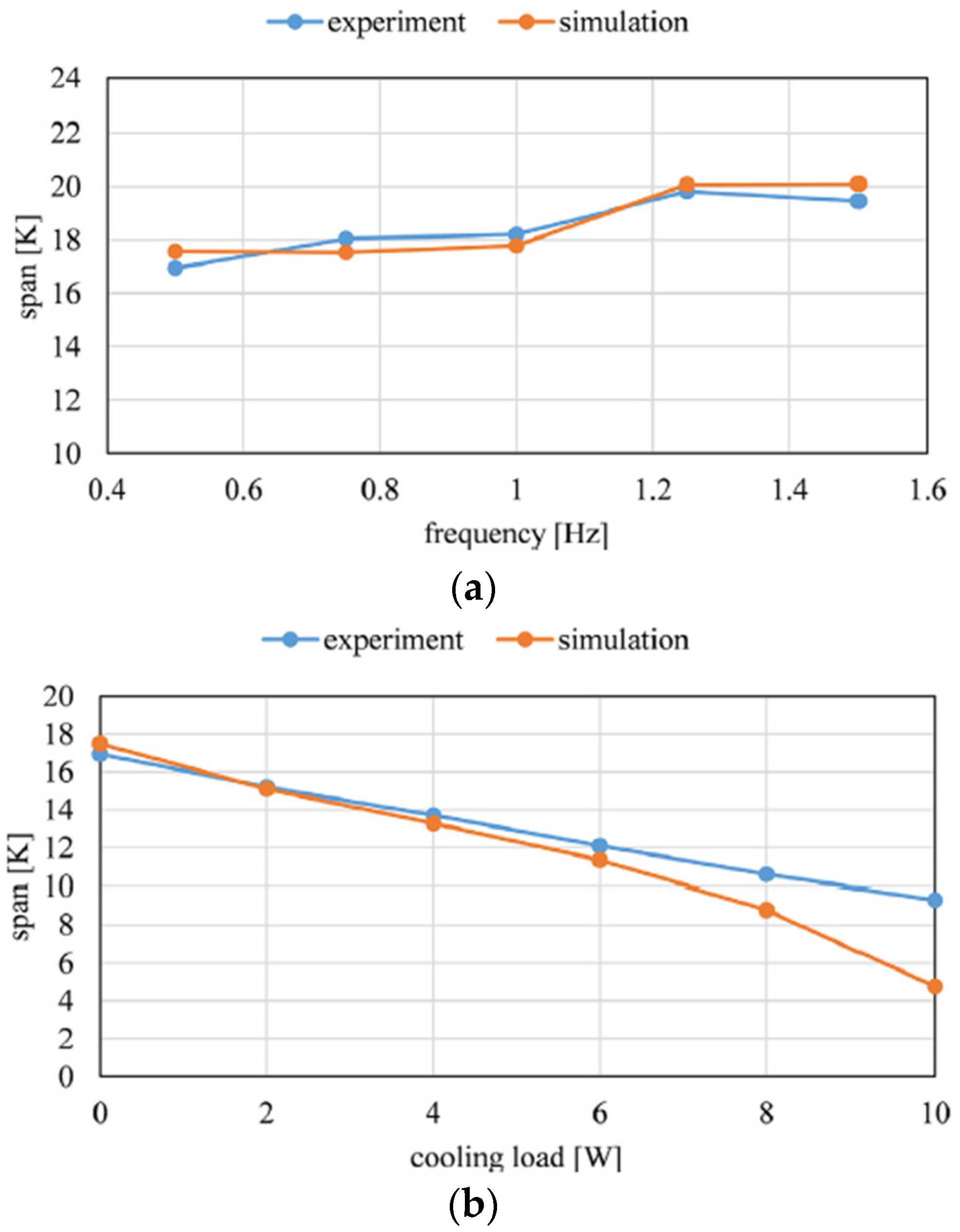
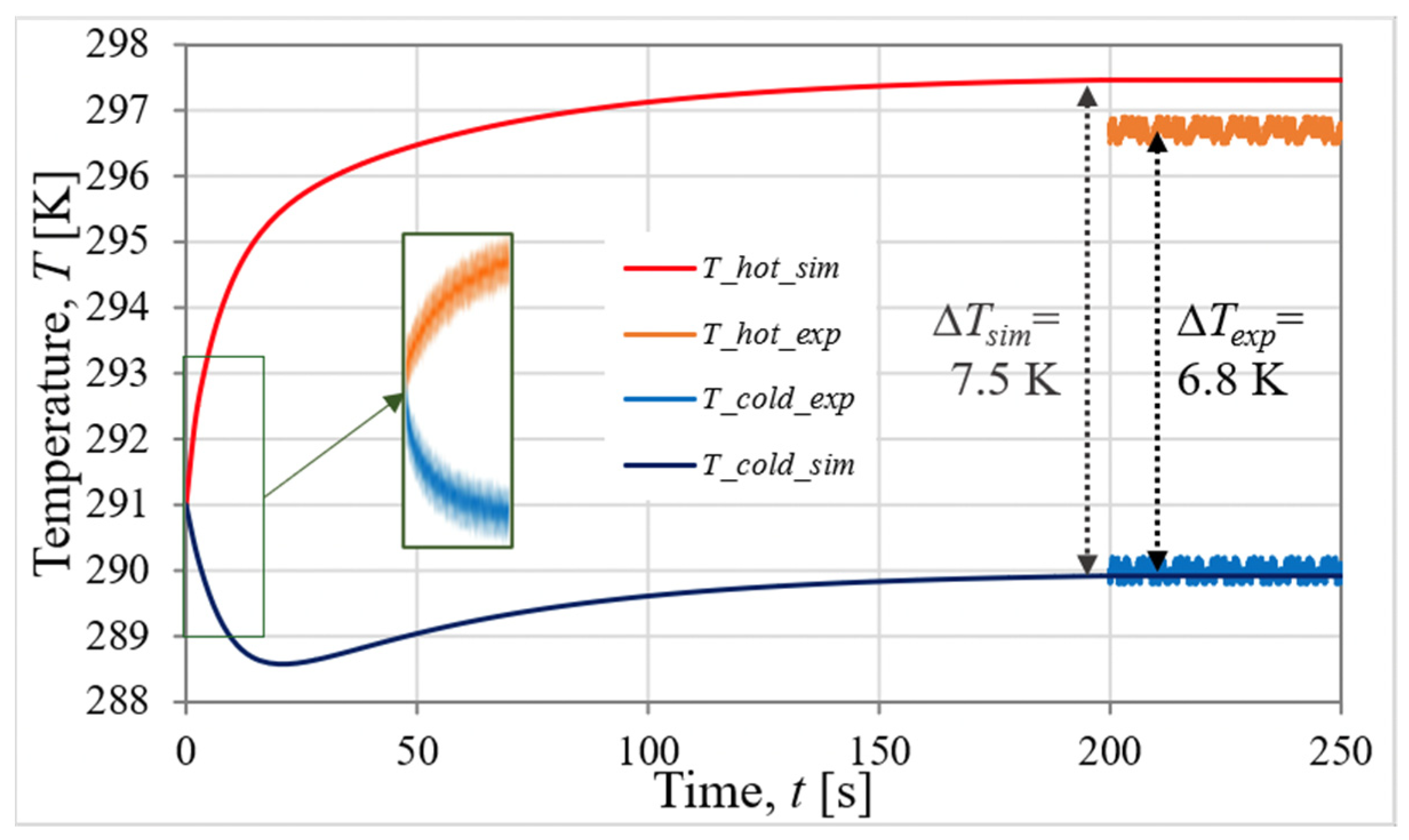
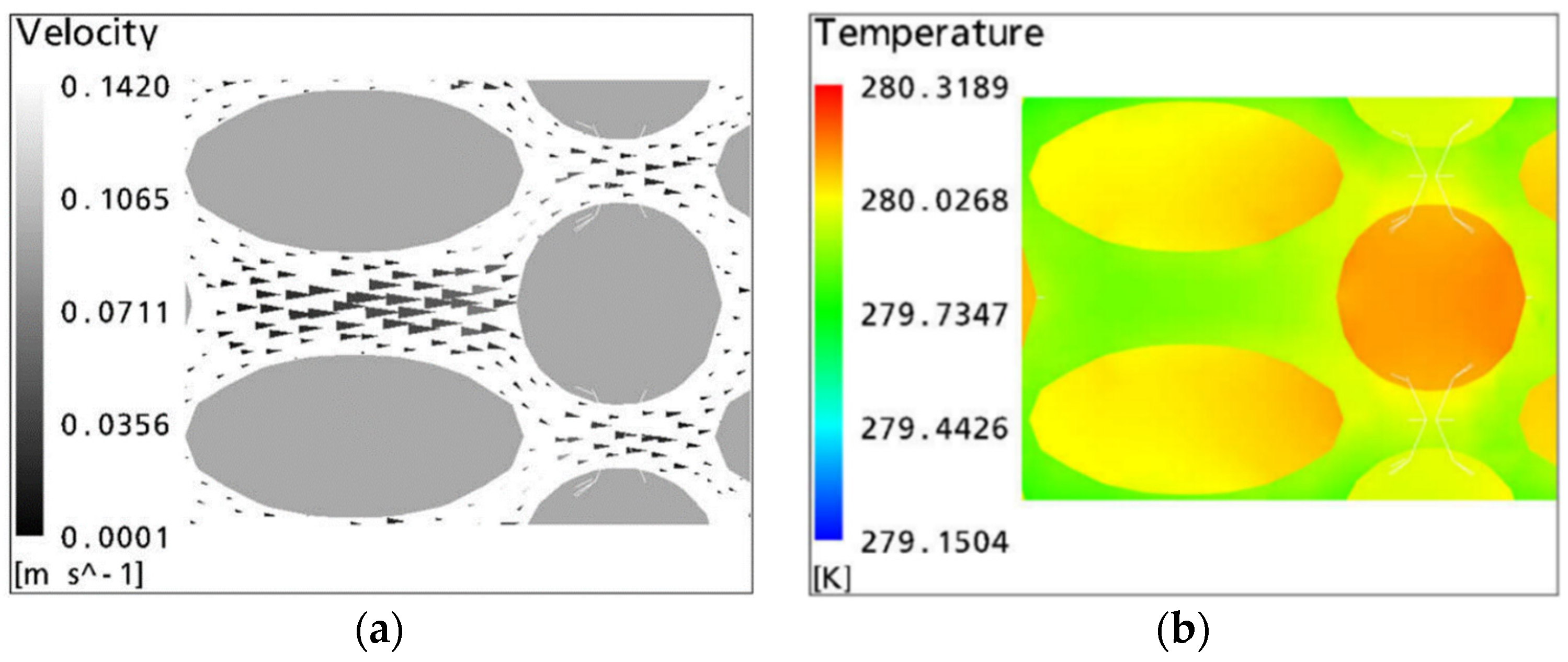
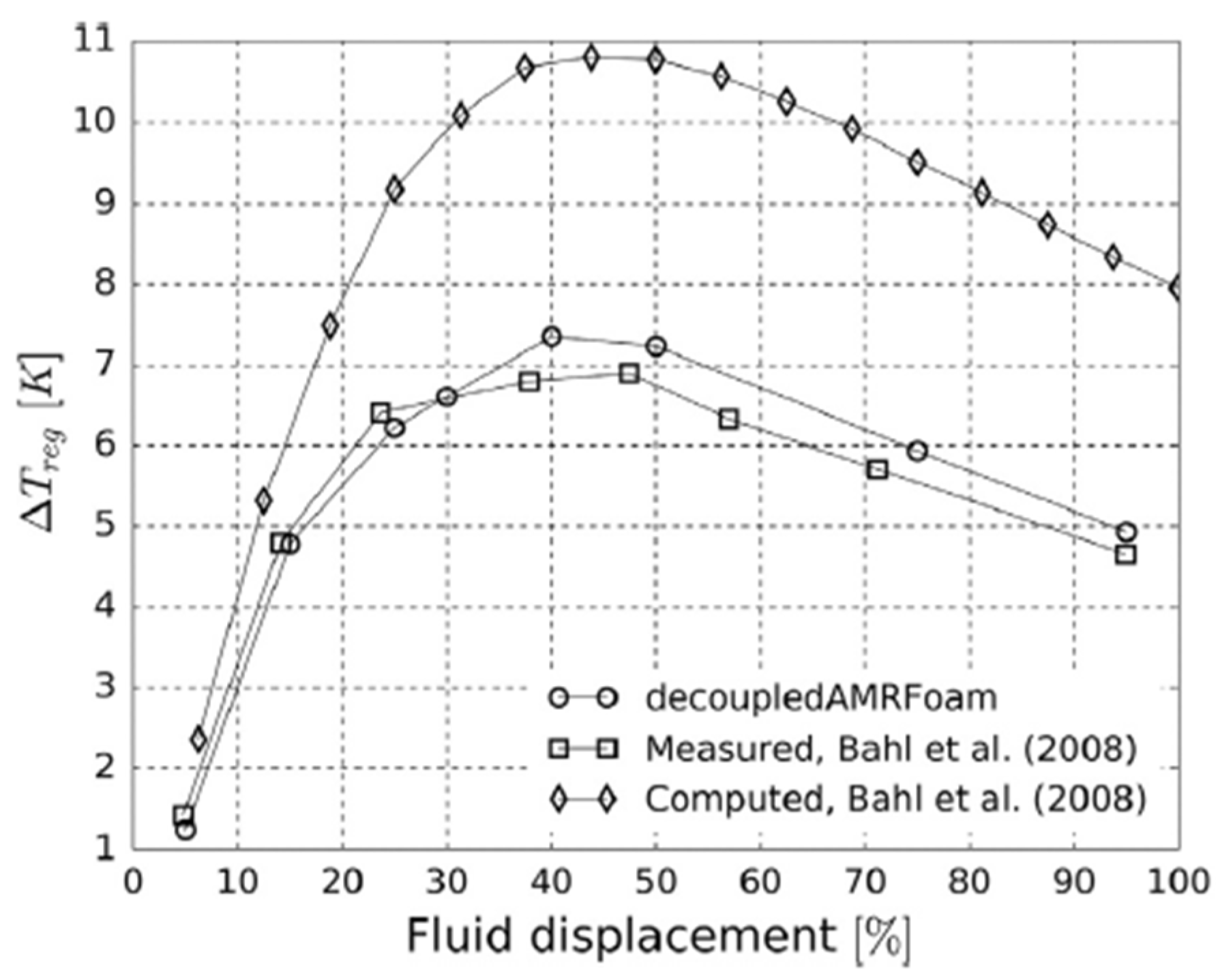
Table 1.
Models’ synthesis and characteristics.
| Authors, Year, References | Model Type, n-D | Physical Coupling | Magnetic Field Source, Movement 1 | Geometry of the Studied MCM | Validation | Description |
|---|---|---|---|---|---|---|
| Smaïli and Chahine, 1998 [52] | Semi-analytical, 1-D | Thermo-fluidic | Porous matrix | Study of MCM composite and thermodynamical cycle. | ||
| Allab et al., 2005 [53] | Semi-analytical, 1-D | Thermo-fluidic | PM, translation | Gd thin plate | Experimental | Study on the AMRR cycle. |
| Dikeos et al., 2006 [54] | Semi-analytical, 1-D | Thermo-fluidic | SM, translation | Gd puck | Experimental | Simulation of an AMRR test device. |
| Sarlah et al., 2006 [55] | Semi-analytical, 2-D | Thermo-fluidic | PM, rotary | Gd honeycomb | Study on the four steps of an AMRR. | |
| Bouchekara et al., 2008 [56] | Semi-analytical, 1-D | Thermo-fluidic | Gd plates | Numerical | Inverse problem optimization method to design an AMRR. | |
| Petersen et al., 2008 [57] | Semi-analytical, 2-D | Thermo-fluidic | PM, translation | Gd parallel plates | Numerical | Study on parallel plates with a 2-D model. |
| Engelbrecht et al., 2008 [58] | Semi-analytical, 1-D | Thermo-fluidic | PM, translation | Three parallel plates | Experimental and numerical | Model considering the mechanical losses. |
| Nielsen et al., 2009 [59] | Semi-analytical, 2.5-D | Thermo-fluidic | PM, translation | Gd parallel plates | Experimental | Improvement of Petersen’s model. |
| Bouchard et al., 2009 [60] | Semi-analytical, 3-D | Thermo-fluidic | Gd spheres particles | Experimental | Study on a porous regenerator. | |
| Tagliafico et al., 2010 [61] | Semi-analytical, 1-D | Magneto-thermo-fluidic | Gd | Parametric study on the AMRR performances. | ||
| Risser et al., 2010 [62] | Semi-analytical, 1-D | Magneto-thermo-fluidic | PM | Gd parallel plates | Study of a MC system for an industrial application. | |
| Sarlah and Poredos, 2010 [63] | Semi-analytical, 1-D | Thermo-fluidic | Gd spherical particles | Experimental | Study on a dimensionless model. | |
| Liu and Yu, 2011 [64] | Semi-analytical, 2-D | Magneto-thermo-fluidic | Gd packed bed | Experimental and numerical | Study on the AMRR performances and temperature distribution. | |
| Tušek et al., 2011 [65] | Semi-analytical, 1-D | Thermo-fluidic | Packed bed Gd spheres | Study on a large AMRR operating conditions. | ||
| Rowe, 2012 [66,67] | Semi-analytical, 1-D | Magneto-thermo-fluidic | Experimental | Model to study the AMRR thermodynamics. | ||
| Vuarnoz and Kawanami, 2012 [68] | Semi-analytical, 1-D | Thermo-fluidic | PM, translation | Stack of Gd wires | Experimental | Model to study an AMRR geometry. |
| Oliveira et al., 2012 [69] | Hybrid (analytical and numerical), 2-D | Thermo-fluidic | PM | Gd parallel plates | Experimental | Focus on the fluidic phenomena in the regenerator. |
| Canesin et al., 2012 [70] | Semi-analytical, 2-D or 3-D | Thermo-fluidic | Analytical and numerical | Open source CFD program to study AMRR geometry. | ||
| Risser et al., 2013 [71] | Semi-analytical and numerical, 1-D and 3-D | Magneto-thermo-fluidic | PM | Gd parallel plates | Experimental | Enhanced model to increase the design efficiency of future model. |
| Aprea et al., 2013 [72] | Semi-analytical, 1-D | Thermo-fluidic | Comparison between SOMT and FOMT energy performances. | |||
| Mira et al., 2014 [73] | Semi-analytical and numerical, 1-D | Magneto-thermo-fluidic | EM, static | Gd parallel plates | Experimental | Multi-physics model, applied to a test bench. |
| Burdyny et al., 2014 [74] | Semi-analytical, 1-D | Magneto-thermo-fluidic | PM, rotary | Gd spheres | Experimental and numerical | Performance of a single-material AMRR with a good accuracy. |
| Hsieh et al., 2014 [75] | Semi-analytical, 2-D | Thermo-fluidic | Segments of Gd and GdTb | Focus on a graded AMRR performance. | ||
| Nikkola et al., 2014 [76] | Semi-analytical, 1-D | Thermo-fluidic | A model to study AMRR on Matlab® with a Graphical user interface. | |||
| Lei et al., 2015 [77] | Semi-analytical, 1-D | Thermo-fluidic | PM | Packed particles bed of La(Fe,Mn,Si)13Hy | Experimental | An AMRR model to study multi-layered regenerator performances. |
| Lionte et al., 2015 [78] | Semi-analytical, 2-D | Thermo-fluidic | PM | Gd parallel plates | Experimental | Simulation performance of a test bench. |
| Park et al., 2015 [79] | Semi-analytical, 1-D | Thermo-fluidic | SM | Experimental | Model of a two-stage AMRR with 2 MCM for each stage. | |
| Trevizoli et al., 2016 [80,81] | Semi-analytical, 1-D | Thermo-fluidic | PM, rotary | Gd spheres | Experimental | Mathematical modeling to determine the thermal losses for cooling applications. |
| Niknia et al., 2016 [82] | Semi-analytical, 1-D | Thermo-fluidic | PM | Gd spheres | Experimental | Study on the external losses. |
| Schroeder and Brehob, 2016 [83] | Semi-analytical, 1-D | Thermo-fluidic | Gd parallel plates | Experimental | New four cycles consideration of the AMRR processes. | |
| Mugica et al., 2017 [84] | Semi-analytical, 1-D | Magneto-thermo-fluidic | PM, translation | Gd parallel plates | Experimental and numerical | The addition of insulator layers within the MCM increases the temperature span. |
| Roy et al., 2017 [85] | Semi-analytical, 1-D | Thermo-fluidic | Gd parallel plates | Experimental | A model coupled with a genetic algorithm to study parallel plate AMRR. | |
| Plait et al., 2018 [86,87] | Semi-analytical and numerical, 2-D | Magneto-thermo-fluidic | EM, static | Gd parallel plates | Experimental | Multi-physics model, application to a test bench. |
| Monfared, 2018 [88] | Semi-analytical, 1-D and 3-D | Magneto-thermo-fluidic | PM, rotary | Packed bed of Gd particles | Experimental | Multi-physic model to design and optimize a rotary AMRR device. |
| Mugica et al., 2018 [89] | Semi-analytical, 3-D | Magneto-thermo-fluidic | PM | Random packed bed particles | Experimental | An original solver to study random AMRR of packed bed particles. |
| Teyber et al., 2019 [90] | Semi-analytical, 1-D | Thermo-fluidic | PM | Experimental | Semi-analytic AMRR model with Phyton ScyPy package. | |
| Silva et al., 2019 [91] | Semi-analytical, 1-D | Thermo-fluidic | PM, translation | Numerical | Development of the python framework: HEAt TRAnsfer in Python (HEATRAPY). | |
| Vieira et al., 2021 [92] | Semi-analytical, 1-D | Thermo-fluidic | La(Fe,Mn,Si)13Hy spheroidal particles | Experimental | Study of the La(Fe,Mn,Si)13Hy properties and performances in an epoxy-bonded AMRR. |
1 Determination of the type of motion of the magnetic field source considered by the studied geometry of the model. Most of the time, the utilization of PM or SM requires a movement (translation or rotation for example) and an EM can be used without motion. These motions can carry out the cycles of magnetization and demagnetization.
Publisher’s Note: MDPI stays neutral with regard to jurisdictional claims in published maps and institutional affiliations. |
© 2021 by the authors. Licensee MDPI, Basel, Switzerland. This article is an open access article distributed under the terms and conditions of the Creative Commons Attribution (CC BY) license (https://creativecommons.org/licenses/by/4.0/).
Share and Cite
MDPI and ACS Style
Eustache, J.; Plait, A.; Dubas, F.; Glises, R. Review of Multi-Physics Modeling on the Active Magnetic Regenerative Refrigeration. Math. Comput. Appl. 2021, 26, 47. https://0-doi-org.brum.beds.ac.uk/10.3390/mca26020047
AMA Style
Eustache J, Plait A, Dubas F, Glises R. Review of Multi-Physics Modeling on the Active Magnetic Regenerative Refrigeration. Mathematical and Computational Applications. 2021; 26(2):47. https://0-doi-org.brum.beds.ac.uk/10.3390/mca26020047
Chicago/Turabian StyleEustache, Julien, Antony Plait, Frédéric Dubas, and Raynal Glises. 2021. "Review of Multi-Physics Modeling on the Active Magnetic Regenerative Refrigeration" Mathematical and Computational Applications 26, no. 2: 47. https://0-doi-org.brum.beds.ac.uk/10.3390/mca26020047