
A Novel Reconstruction Method to Increase Spatial Resolution in Electron Probe Microanalysis


Research Lab for Applied and Computational Mathematics (ACoM), Department of Mathematics, RWTH Aachen University, Schinkelstr. 2, 52062 Aachen, Germany
*
Author to whom correspondence should be addressed.
Math. Comput. Appl. 2021, 26(3), 51; https://0-doi-org.brum.beds.ac.uk/10.3390/mca26030051
Submission received: 17 May 2021
/
Revised: 4 July 2021
/
Accepted: 9 July 2021
/
Published: 14 July 2021
Abstract
:The spatial resolution of electron probe microanalysis (EPMA), a non-destructive method to determine the chemical composition of materials, is currently restricted to a pixel size larger than the volume of interaction between beam electrons and the material, as a result of limitations on the underlying k-ratio model. Using more sophisticated models to predict k-ratios while solving the inverse problem of reconstruction offers a possibility to increase the spatial resolution. Here, a k-ratio model based on the deterministic M1-model in Boltzmann Continuous Slowing-Down approximation (BCSD) will be utilized to present a reconstruction method for EPMA which is implemented as a PDE-constrained optimization problem. Iterative gradient-based optimization techniques are used in combination with the adjoint state method to calculate the gradient in order to solve the optimization problem efficiently. The accuracy of the spatial resolution still depends on the number and quality of the measured data, but in contrast to conventional reconstruction methods, an overlapping of the interaction volumes of different measurements is permissible without ambiguous solutions. The combination of k-ratios measured with various electron beam configurations is necessary for a high resolution. Attempts to reconstruct materials with synthetic data show challenges that occur with small reconstruction pixels, but also indicate the potential to improve the spatial resolution in EPMA using the presented method.
1. Increasing the Spatial Resolution in EPMA
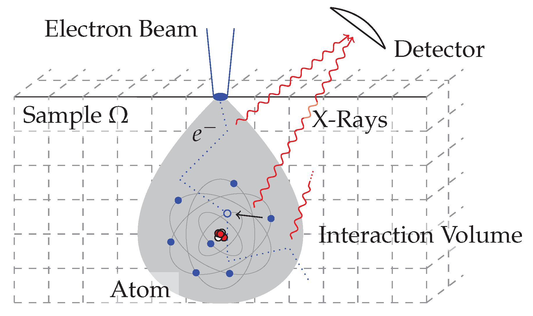
Electron probe microanalysis (EPMA) [1,2] is a non-destructive method to determine the chemical composition of a material sample that is applied in various fields, for example geophysics, material science, or engineering. The composition is not measured directly, but reconstructed from the intensity of X-rays, which are produced by exciting a material sample with a focused beam of electrons. Atoms inside the sample are ionized by collision with the highly energetic beam electrons and subsequently relax from the excited state by emitting characteristic X-ray radiation. A part of the radiation is absorbed, the other part leaves the sample and is measured by a detector. The characteristic radiation is quantified in the form of k-ratios , where the measured radiation intensity I is normalized by standard intensities measured for a known reference sample. A sketch of the physical processes is shown in Figure 1.
We characterize the chemical composition of a material by its mass fraction field . Due to the statistical nature of the k-ratio measurements, the mass fractions , as the solution to the inverse problem of reconstruction, are also probabilistic and all information gained by the experiment is encoded in the statistical moments of [3]. However, the probabilistic inversion is challenging; thus, this article deals with the minimization of the squared error of k-ratios obtained from an experiment and a forward model . The result can be interpreted as a maximum likelihood estimate under the assumption that the noise of the experimental data is independent and identically Gaussian distributed.
A parametrization that restricts the unknown to finite dimensions states a regularization of the generally ill-posed inverse problem. The minimization can then be written as
Currently, forward models typically used in reconstruction (ZAF, ) [2,4,5,6,7] assume either a fully homogeneous or a layered structure interaction volume (the part of the sample in which beam electrons excite atoms). The ZAF model uses correction factors for the atomic number , the absorption , and the fluorescence and is implemented as a fixed-point iteration to reconstruct homogeneous mass fractions from k-ratios obtained from a single beam configuration. This idea is extended to layered samples using a correction model based on the depth distribution of X-ray generation . The material is scanned by the electron beam, ensuring that their interaction volumes do not overlap, and each interaction volume is reconstructed independently. In this procedure, the forward models limit the size of the reconstruction pixels to a size that corresponds approximately to the size of the interaction volume.
Previous analysis [8,9,10] of the analytical spatial resolution highlight the need to resolve small structures inside the sample, e.g., the inclusion of spherical droplets in lunar rock which forms due to exposure to energetic particles or small crystals of magnetite embedded in glass. In [8,9,10], the analytical spatial resolution of EPMA is defined as the size of the interaction volume and approaches which physically decrease this volume are described. In contrast, we propose to decouple the spatial resolution and the size of the interaction volume by employing a more sophisticated reconstruction method that harnesses k-ratio measurements from multiple experiments with overlapping interaction volumes.
To analyze the size of the interaction volume of inhomogeneous structures, Monte Carlo models [11,12,13,14,15] are used. Additionally, Monte Carlo models can be used to implement a k-ratio model that allows inhomogeneous material structures by first estimating the electron transport on the basis of Monte Carlo sampling and then approximating the measured X-ray intensity. However, Monte Carlo models suffer from statistical noise which restricts the use of gradient based optimization techniques to solve the inverse problem [16].
In this work, we use a deterministic k-ratio model that bases on the [16,17,18,19,20] in Boltzmann Continuous Slowing-Down approximation (BCSD) and is able to deal with inhomogeneous interaction volumes. The model has previously been validated against Monte Carlo models [16]. Our model additionally allows a fast and precise gradient computation via the adjoint state method, hence efficient gradient based optimization techniques can be applied. The combination of a deterministic model and gradient based optimization methods allows the implementation of a reconstruction method with a higher spatial resolution. Instead of prohibiting overlapping interaction volumes, this method merges sequential k-ratio measurements with multiple beam configurations to accomplish a higher resolution with a pixel size smaller than the size of the interaction volume.
The source code accompanying this article is made available via GitHub: https://github.com/tam724/m1epma (accessed on 9 July 2021) [21].
2. Deterministic k-Ratio Model
2.1. Parameterized Material Description
A sample occupying a domain , which consists of chemical elements, is characterized by the mass fractions of all elements at every point . The mass fraction
describes the ratio of partial to total mass in a (infinitesimal small) volume around for one element and is therefore constrained by and . The choice of a global set of parameters discretizes the mass fractions and limits the unknown to finite dimensions.
In this work, the mass density is modeled by a linear combination of the mass fractions and the density of the pure elements. Such a model neglects the influence of different molecular structures and assumes that only mass fractions sufficiently describe the material.
2.2. k-Ratios as a Function of the Electron Number Density
The measured quantities in EPMA, the radiation intensities of X-rays with wavelengths characteristic to elements occurring in the material, are considered in terms of k-ratios . The measured intensity I gets normalized by the intensity measured for a known reference sample, to account for experimental inaccuracies, e.g., the detector efficiency. Furthermore, an experiment is conducted with setups (here, we consider different beam energies and beam positions) yielding different measurements. An enumeration of all k-ratios allows for collecting all measured k-ratios into .
We model a k-ratio by
representing the integral of the zeroth moment of the electron fluence over the spatial domain and all considered energies , weighted by attenuation and emission/fluorescence factors. The presence of element i at a position is taken into account by the number density of atoms per unit volume , with the atomic mass . The ionization cross-section , which combines fluorescence yield and ionization cross-section, describes the fraction of electron-atom collisions leading to X-ray generation. X-ray attenuation is approximated by the Beer–Lambert law with the linear attenuation coefficient being averaged over paths from each point to the detector. The attenuation coefficient of a compound affecting an X-ray j is given by . Emission cross-section and mass attenuation coefficients are interpolated from tabulated data; for details, see [22,23,24,25]. Note that the integrals in Equation (3) model the intensity ; hence, the standard intensities can also be calculated this way by inserting the respective mass fractions.
2.3. M1-Model of Electron Transport
To model , we use the [16,17,18,19,20] in BCSD, which describes the first two moments of the electron fluence inside the material. They are defined as
using the velocity of electrons (with magnitude defined by the electron energy and direction ) and the stationary number density of electrons . Based on the Boltzmann equation in Continuous Slowing-Down approximation, the belongs to a class of models which are derived from closing the system of moments by minimization of the Boltzmann entropy. With a closure after the first moment, , the system takes the form of a nonlinear hyperbolic partial differential equation (PDE) in space and energy, given by
Thereby, is the anisotropy parameter and is the Eddington factor, which implicitly depends on and is approximated by a rational function. The identity matrix is denoted by . Stopping power S and transport coefficient T for a compound are obtained from the mass fractions , the density , and the respective coefficients of pure elements and :
The analytic forms of , and the function that approximates as well as the Jacobian of the flux function are given in Appendix A. For a detailed description of the , we refer to [16,17,18,19,20]. A solution of the depends on the material parameters because stopping power and transport coefficient depend on the mass fractions which are parameterized by .
Boundary Conditions
Initial and cutoff energy of the computational domain are chosen such that the beam is sufficiently captured and all minimal ionization energies are considered . The edge energy of an element i is the lowest energy at which ionization still occurs. Initially, no beam electrons are present inside the domain , hence
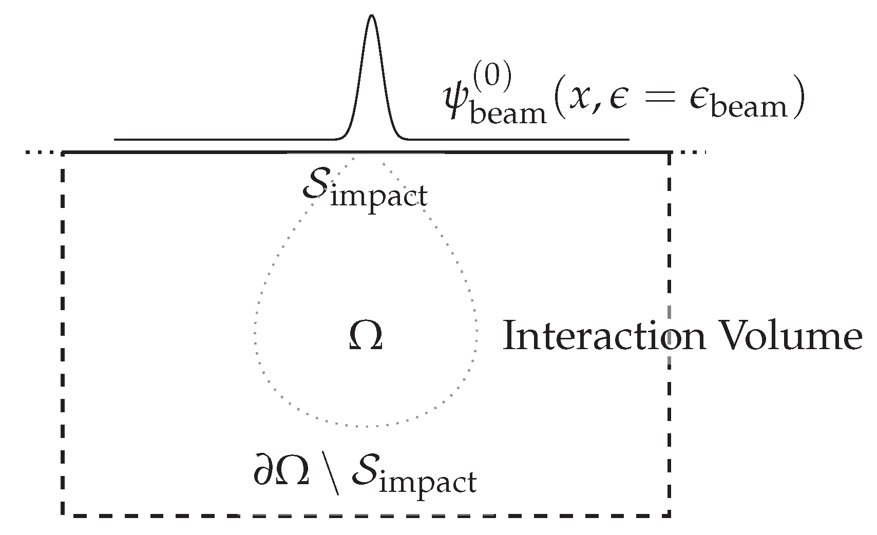
The spatial boundary consists of one surface that corresponds to the samples surface where the electron beam impacts. The other boundaries lie inside the sample and are assumed to be sufficiently far from the interaction volume so as not to influence the solution. A schematic of the 2D setup is provided by Figure 2. The electron beam is modeled as Gaussian in space and energy and Dirac in angle, yielding the moments
where is a unit vector describing the direction of the beam, the normal distribution, given the respective means, and , and variances, and . This leads to the following spatial boundary condition:
which will in the following be referred to as for multiple beam configurations .
3. Inverse Problem of Material Reconstruction
3.1. PDE-Constrained Optimization Problem
Given measured k-ratios , the reconstruction of material parameters can now be written as a PDE-constrained optimization problem. Incorporating the k-ratio model, consisting of the integral equation (Equation (3)) and the G (Equation (5)) with boundary conditions , the inverse problem of reconstruction is:
This reads as follows. Find the parameters such that the objective function , the least-squares error of the residuals between modeled and measured k-ratios, is minimal. Later, we will refer to the residuals as . Here, the moments of the electron fluence , which are used to determine the k-ratios , are subject to the implicit constraint to fulfill the with its boundary conditions . To obtain a set of k-ratios , a solution of the PDE-constaints is calculated and integrated according to Equation (3).
Note the direct influence of the mass fraction parameters on the modeled k-ratios via Equation (3) and the indirect influence via the moments of the electron fluence . Therefore, a perturbation in will not only change the objective function H due to their direct dependency, but also due to the implied perturbation in .
3.2. Iterative Gradient Based Optimization
To find a solution to the inverse problem, an iterative optimization method of the form starting with an initial guess is used. Many optimization methods calculate the update based on the gradient of the objective function and possibly also higher order derivatives—for example, using the negative gradient of the objective in combination with a line search method to find the step length yields the method of steepest descent [29]. The Levenberg–Marquardt [29] algorithm additionally exploits the least-squares form of the objective function and can be interpreted as a combination of a gradient descent approach on the objective function H and a Gauss–Newton method acting on the residuals . In contrast to the method of steepest descent, which only requires the evaluation of the objective function H and its gradient, the Levenberg–Marquardt method additionally needs the computation of the Jacobian of the residuals with respect to . In [29,30], these two and several other methods of a similar form are extensively described, with most methods sharing the need to calculate derivatives. Note that such methods only converge to a local optimum and do not guarantee a global minimization.
For the PDE-constrained problem (10), the cost of such methods is dominated by the cost of evaluating the PDE-constraint as part of the objective function and the cost of evaluating its derivatives. It is advantageous to choose an optimization method which requires a low number of evaluations of the objective function and its derivatives, but the efficiency of each evaluation still remains crucial. A naive approach to determine the derivative is a finite difference approximation, which, applied to our problem, requires at least evaluations of the objective function. Each evaluation of the objective function includes solving computationally expensive PDEs. Given many parameters or experimental setups , which are required for high resolution, this approach becomes computationally too expensive. Furthermore, the choice of the spacing for the finite difference approximation is non-trivial. Another option to determine derivatives is the implementation of additional sensitivity equations [31] besides the PDE-constraint. However, the cost also scales with the number of parameters in this case, which inhibits their application for our problem.
3.3. The Adjoint State Method
The adjoint state method provides an alternative to calculate the gradient. Details on the method can be found in [31,32,33], while here we give the general steps that will later be needed to apply it for problem (10).
The Levenberg–Marquardt method requires the Jacobian of the residuals , while, for the steepest descent, the gradient of the objective H is needed. Covering both cases, we consider the gradient of a scalar valued functional with respect to . The functional h could be one component of the residual , to gradually calculate the Jacobian for the Levenberg–Marquardt method, or the objective H for the gradient used in steepest descent. Without loss of generality, but, for simpler notation, the discussion here is limited to only one PDE constraint where we consider the state variable , which is implicitly related to the parameters by (omitting the index k for the beam configurations).
The introduction of a Lagrange multiplier, the adjoint state variable , allows for stating the Lagrange function of the optimization problem:
Here, denotes the scalar product in function spaces, is the scalar product in . For , one recognizes the equality of and h, which implies the equality of their gradients .
Consider the directional derivative of the Lagrangian in a direction . Using , the direction of change of the state variable corresponding to a small perturbation of the parameters, such that , the directional derivative can be written as
Here, denotes the functional derivative, the vector of partial derivatives with respect to , not including the variation due to , and the corresponding Fréchet derivative operators. Multiple calculations of Equation (12), while iterating over the unit vectors as direction , accumulate to the gradient , but would include multiple expensive calculations of the direction . To avoid this calculation, Equation (12) is rearranged to
where is the adjoint operator of the Fréchet derivative . The crux of the adjoint state method is to force to satisfy the adjoint state equation
such that the first scalar product in Equation (13) including vanishes and only the second scalar product remains as the directional derivative of . Then, the gradient is identified as
To calculate the full gradient, one evaluation of the adjoint state Equation (14) is sufficient because it does not depend on the direction . Its structure is usually similar to the structure of the forward equation but depends on the specific form of the adjoint operator. Being an essential component of the method, the adjoint operator for our problem (Equation (10)) will now be derived under consideration of the form of the PDE-constraint G (Equation (5)).
3.4. Adjoint State Method for the M1-Model Constraint
The adjoint state method bases on the identity
The adjoint operator allows for isolating the direction in the scalar product of Equation (13), which subsequently enables stating the adjoint state Equation (14). To derive the adjoint state equation for the , this identity must be considered, taking G from Equation (5) into account. The Fréchet derivative of G can be found using the Jacobians of the flux functions . Inserting into Equation (16) and proceeding using integration by parts yields
The boundary integrals, which are enforced to be zero, yield boundary conditions for the adjoint state variable . At energy , the state variable is specified by the boundary condition of the which does not depend on the parameters ; therefore, . At energy , we have to prescribe the adjoint state variable . In addition, the boundary term for the spatial boundary with outer normal vector has to vanish, which yields boundary values for on . Their numerical implementation is discussed along with the boundary conditions for the forward model in Section 4.
Then, the adjoint state equation to be solved for the adjoint state variable is given by
To solve the adjoint equation, the solution of the forward equation has to be known, since and depend on it.
The term acts as a source to the adjoint state variable and depends on the choice of the functional h to be differentiated. For the Levenberg–Marquardt algorithm, the calculation of the gradient of each residual is required, thus we choose . Since in Equation (3) the first component of the state variable enters the integral linearly, the functional derivative of one residuum is given by
Here, collects all weighting factors of the integral in Equation (3).
To implement the steepest descent method, the gradient of the objective H is required; therefore, and, by a similar argument as above, its functional derivative is
Having the adjoint equation determined by the adjoint operator and the respective source for the adjoint state variable, the calculation of the gradient via the adjoint state method can be summarized by
- the solution of the forward equation for ,
- the solution of the adjoint Equation (18) for and
- the calculation of the gradient
In comparison to a finite difference approximation with solutions of a PDE, the adjoint state method only requires the solving of the forward (first step) and the adjoint (second step) equation to calculate the gradient. The calculation of the gradient (third step) can usually be implemented efficiently. Consequently, the adjoint state method offers an efficient way to determine the gradient to be used in an iterative optimization method for our problem (10).
4. Numerical Implementation
4.1. Material Parameterization
The subdivision of the material into reconstruction pixels (see Figure 1) motivates the discretization of the mass fractions as piecewise constant functions. Each parameter describes one of the constant mass fractions in one of the reconstruction pixels. Note that, due to the conditions on (c.f. Section 2), parameters per pixel are sufficient.
4.2. Solving the M1-Model Using Clawpack
The form of Equation (5) motivates the application of finite volume methods to approximate its solution. Our solver of the in two spatial dimensions is implemented using the finite volume library Clawpack/pyclaw [27]. A pseudo time variable transforms the energy interval to be compatible with Clawpack’s formulation. The term can then be split into and , where the first acts like a source term and the second fits to Clawpack’s formulation with S being the capacity function. The capacity coefficient and the source term are applied to the solution via the ‘before-step’ and the ‘source’ function defined by Clawpack. Furthermore, it is important to choose the grid of finite volume cells at least as fine as the reconstruction pixels and to assure that their cell/pixel boundaries coincide.
To implement a Riemann solver, we, as suggested in [26], approximate the Jacobian at each cell interface using the average of the state variable . (See Appendix A.4 for the analytical form of the Jacobian of the flux function .) Then, A is numerically decomposed in eigenvalues and eigenvectors on the basis of which the wave speeds , the wave strengths and right and left going fluctuations and can be identified.
Spatial boundary conditions on are implemented in Clawpack using ghost cells surrounding the computational domain. At the boundary where the beam enters the domain, the ghost cells are updated using Equation (8). The remaining ghost cells are set to zero, justified by the assumption that the computational domain is large enough such that no electrons reach those boundaries.
4.3. Implementation of the k-Ratio Model
Clawpack discretizes the electron fluence into ‘snapshots’ of the solution at specific energies with piecewise constant cell values in space. The spatial integral for the k-ratios k in Equation (3) reduces to a weighted summation over all cells. The attenuation coefficients for each cell is approximated using the path from its midpoint to the detector, which is split in segments overlapping the reconstruction pixels. For the integral in energy, the trapezoidal rule is applied.
4.4. Adaptions to Solve the Adjoint State Equation and Compute the Gradient
Analogous to the , the adjoint Equation (18) is also implemented using Clawpack/pyclaw taking into consideration the reversed direction of computation. Using another pseudo time variable for the adjoint , the term can be written as so that it matches Clawpack’s interface. For the wavespeeds, wavestrengths and fluctuations, the same Riemann solver as for the forward problem is employed. It is only modified to calculate the waves of the transposed Jacobians instead of the Jacobians . To evaluate the Jacobians, the whole forward solution is stored in memory. Via Clawpack’s ‘source’ function, the source term of the adjoint state variable, depending on the required gradient, is integrated. At energy , we choose as the initial condition, while the ghost cells of the spatial boundary are set to Clawpack’s ‘extrapolate’ setting.
5. Numerical Experiments
The following numerical examples illustrate the application of the presented methods and demonstrate their capabilities and limitations. We use synthetic measurements in our experiments which are computed using the same forward model as used for the inversion. The utilized optimization method does not guarantee convergence to a global minimum, and no constraints are enforced on . Overcoming those limitations and implementing a more robust reconstruction method is left for future work.
5.1. Reconstruction on a Small Grid
5.1.1. Zeroth Moment of the Electron Fluence: M1-Model
Under investigation is a domain of a sample consisting of copper and manganese. The domain is partitioned into reconstruction pixels, with a width of , as indicated by the grid in Figure 3. The mass fraction of copper in each cell is randomly chosen from a uniform distribution over ; consequently, the mass fractions of manganese are . The solution of the is computed on a smaller grid with grid cells, with 170 time/energy steps between the initial energy and the cutoff energy .
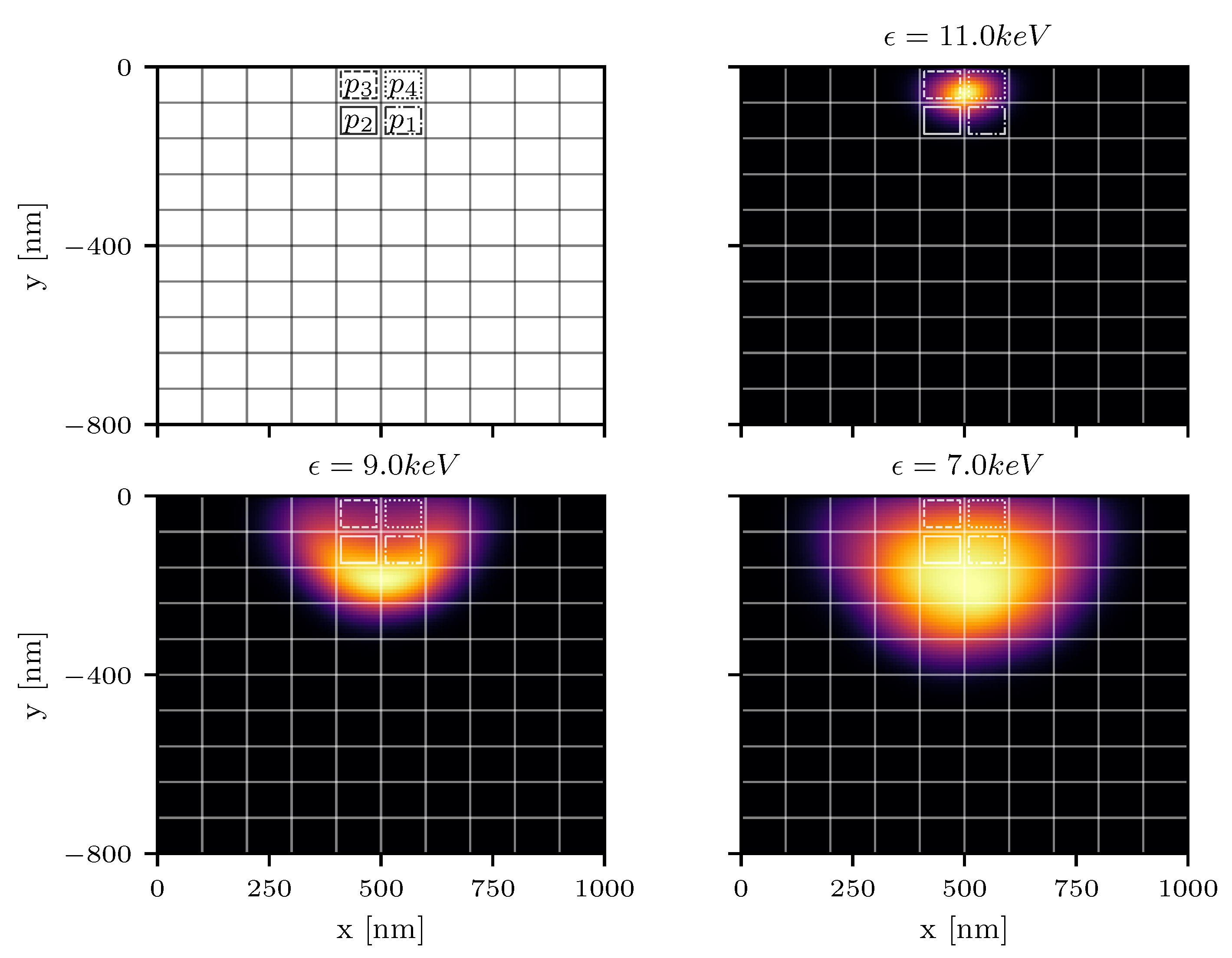
Bombarding this sample with an electron beam from above in a negative y-direction (beam energy , beam position , ), produces the zeroth moment of the electron fluence shown in Figure 3. It displays three snapshots of in energy space as a heat map over the domain . Figure 3 also illustrates the interaction volume, the volume where , which is larger than the reconstruction pixels .
While the number of electrons with high energy is highest near the point of electron impact, electrons with lower energy are more widely distributed in the sample. The contribution of each pixel to the k-ratios scales linearly with the zeroth moment of the electron fluence (Equation (3)), hence a measurement carries most information from pixels close to the surface near the point of electron impact. It is impossible to gain information about the chemical composition in pixels where is zero, so only pixels lying sufficiently close to the surface can be reconstructed.
5.1.2. Convergence to a Particular Solution
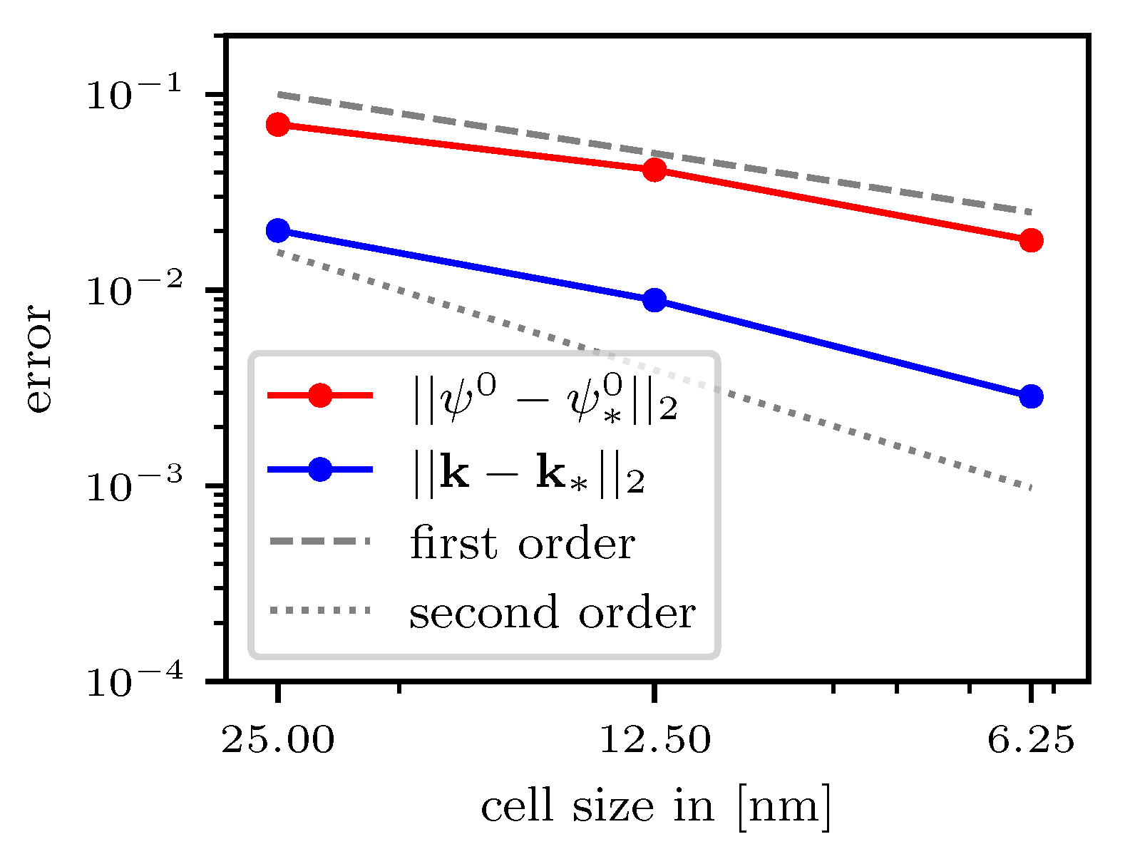
In order to show convergence of the solver and the k-ratio model to a particular solution, we investigate the difference of a solution calculated with different resolutions to a reference solution calculated with high resolution (, cell size: ). Additionally, the k-ratios based on the variable resolution are compared to the k-ratios computed with the high resolution . Figure 4 shows the convergence to the reference solution with decreasing cell sizes. The different resolutions as well as other model parameters are shown in Table 1.
5.1.3. Synthetic Measurements
To mimic a reconstruction problem, we generate synthetic k-ratios ( and ) from the six different beam configurations given by the beam positions and parameters in Table 2. This yields a set of 12 k-ratios, which we consider as synthetic data . All other model parameters are taken from the previous example (Table 1).
5.1.4. Objective Function
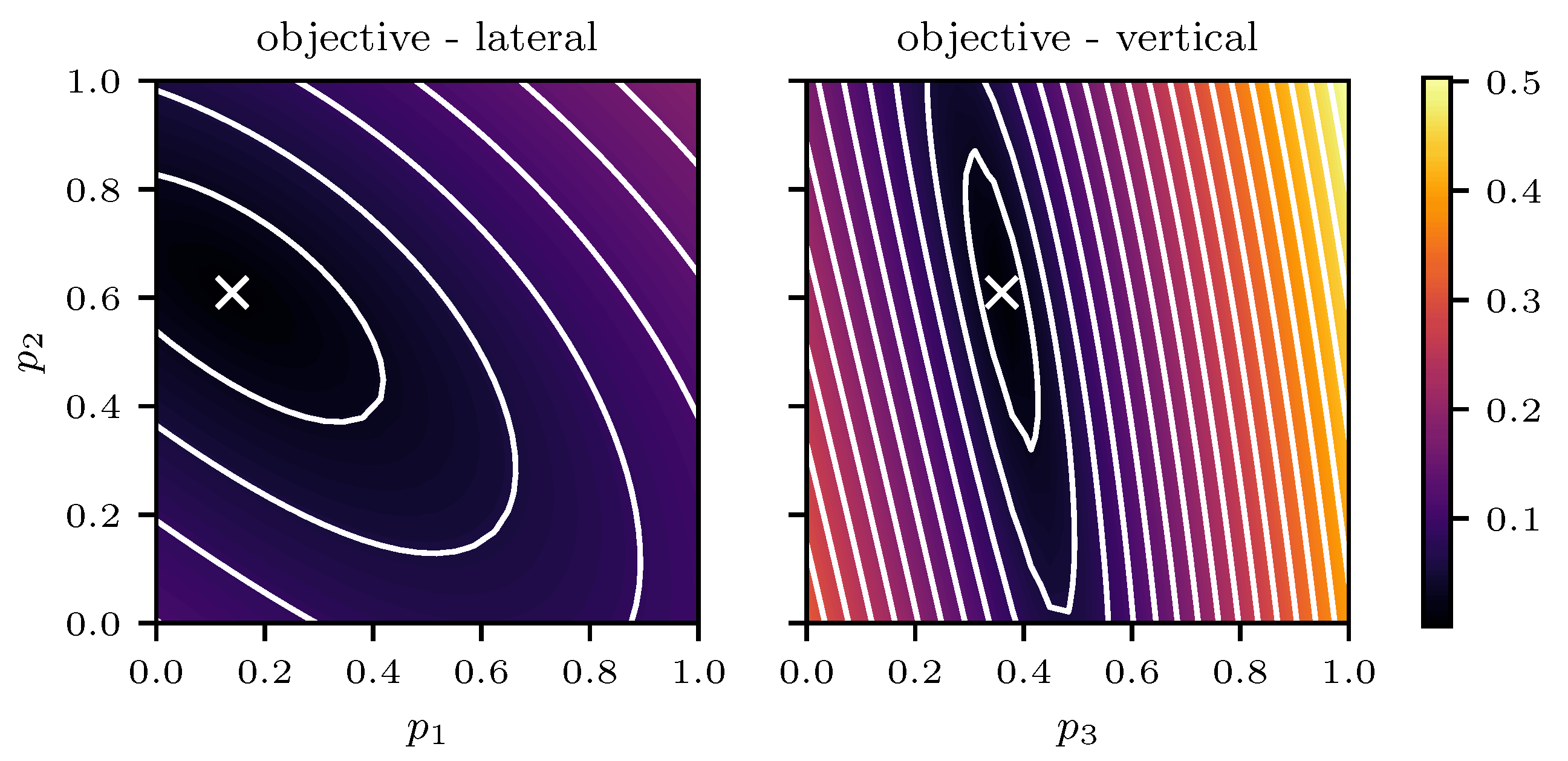
In order to give an insight into the behavior of the inverse problem of reconstruction, we will evaluate the objective function . All k-ratios, synthetic measurements and modeled k-ratios are computed using the same discretization (spatial grid: , energy steps: 100) of the . Both plots in Figure 5 visualize the dependency of the objective function on two of the four parameters describing the mass fractions in the reconstruction pixels. The parameters and describe reconstruction pixels that are next to each other while the pixel belonging to is above that of , cf. the marked cells in Figure 3. The parameters in all other reconstruction pixels are kept to the values used to calculate the synthetic data. The crosses mark the hidden truth, i.e, the parameter values used to calculate the synthetic data. Both contour plots show a unique minimum with a convex objective function, which, however, cannot be expected for the case where all parameters are simultaneously variable. Nevertheless, Figure 5 gives an intuition into the nature of the problem. The shape of the objective function, which increases less rapidly in the direction in which the parameters cancel each other out, e.g., increasing while decreasing , shows that the pixels can partially compensate for each other. It is not detectable in which pixel the x-rays were generated, so an increase in the mass fraction of an element in one pixel may be counteracted to some extent by a decrease in its mass fraction in an adjacent pixel. Therefore, a high spatial resolution can only be achieved by combining measurements obtained from experiments with different electron beam positions and energies.
In addition, the greater elongation in the right plot indicates that it is more difficult to resolve the vertical direction than the lateral direction. The intensity of detected X-rays generated deeper inside the material is lower due to the decreased electron energy and the increased absorption, hence the sensitivity of the k-ratios to changes in the mass fractions of deeper pixels decreases. Using different electron beam energies, the depth of pixels which get excited can be varied and better discrimination of vertical pixels can be achieved. However, the reconstruction of vertical pixels is more difficult than the reconstruction of lateral pixels because, in lateral reconstruction, different electron beam positions can be used to excite only certain pixels. In vertical reconstruction, higher lying pixels are always excited as well.
5.1.5. Reconstruction of Four Parameters
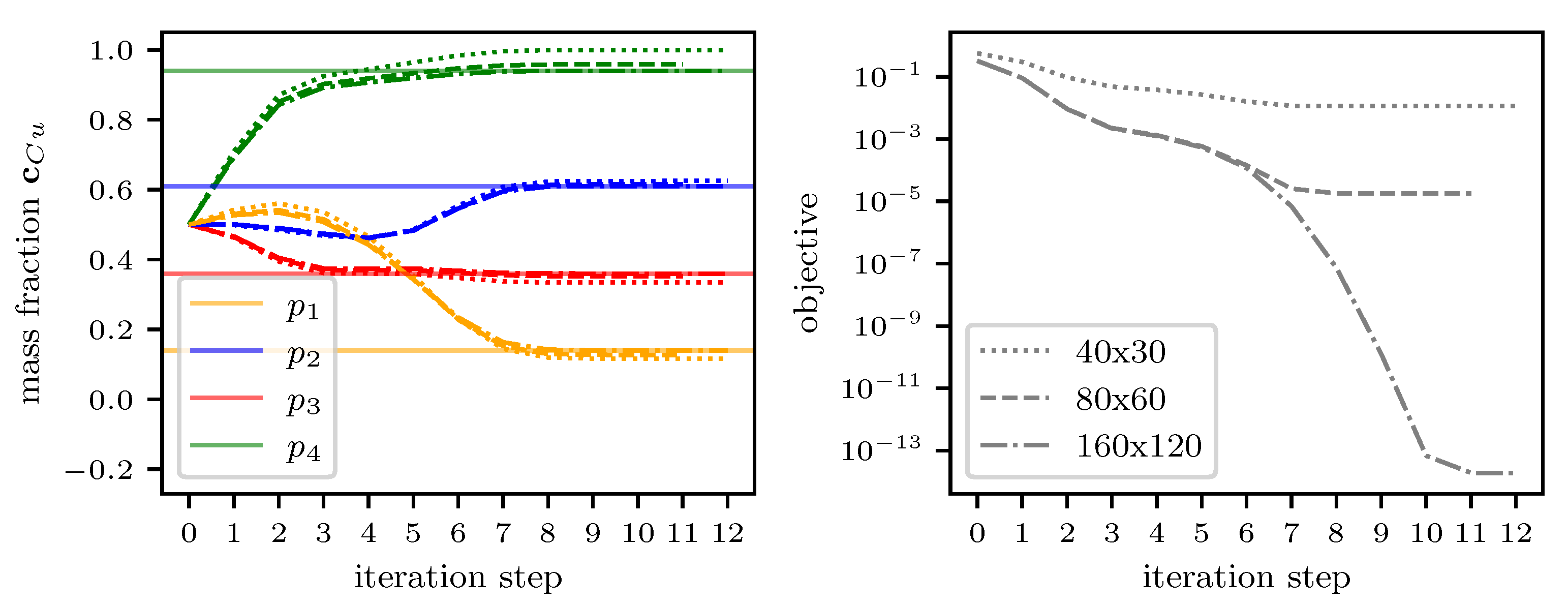
Using the Levenberg–Marquardt optimization algorithm to minimize the objective function of the artificial reconstruction problem yields the optimum illustrated in the left-hand plot of Figure 6, together with the initial values and their evolution during the optimization. Synthetic measurements are computed using the following discretization of the : spatial grid, 300 energy steps. For the reconstruction, multiple discretizations are used: a spatial grid with 70 energy steps, a spatial grid with 100 energy steps and a spatial grid with 300 energy steps.
The hidden truth values are marked with solid lines, which after around 10 steps are identified by the optimization algorithm. The dotted, dashed, and dashdotted lines show the evolution of the parameters during the optimization for the different discretizations. Using the same resolution as used for the synthetic measurements (, dashdotted line) yields a perfect reconstruction. For other resolutions, the reconstructed parameters differ from the hidden truth but converge to similar values. This is due to the fact that the k-ratios also differ when being calculated from the same parameters but with different discretizations. The right-hand plot shows the value of the objective function over the steps of the Levenberg–Marquardt iterations. Again, deviations are visible for different discretizations.
The size of the reconstruction pixel is smaller than the size of the interaction volume (c.f. Figure 3); nevertheless, the iterative reconstruction method is able to reveal the mass fractions. The combination of measurements with different electron beam configurations and overlapping interaction volumes allows the reconstruction with a high spatial resolution.
5.2. Reconstruction on Small Vertical Layers
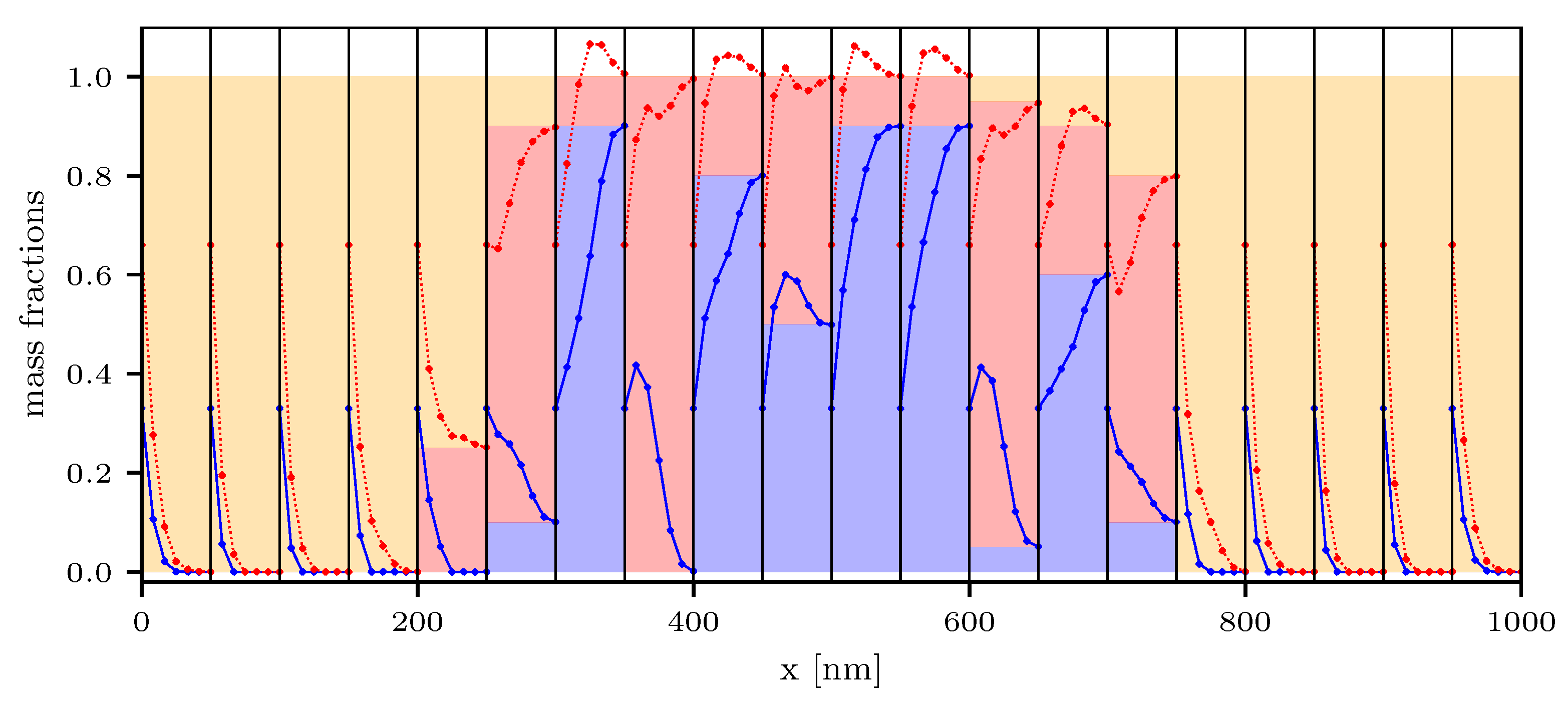
We now consider the reconstruction of a material consisting of iron, nickel, and chromium arranged in vertical layers with a size of , which is smaller than the size of the interaction volume. The material is excited by beams with an energy of and positions centered on each of the vertical layers. All model parameters and discretizations used in this example are given in Table 3. In Figure 7, the iterative reconstruction of the mass fractions is illustrated. The hidden truth configuration of all layers is shown as the background color, where blue is chromium, red is nickel, and the remaining orange part is iron. The Levenberg–Marquardt iterations for the mass fractions of chromium and nickel in each layer are shown by the blue solid and red dotted lines. The mass fraction of iron can be deduced (c.f. Section 2). From the initial configuration (the leftmost point in each layer), all parameters are reconstructed successfully. The rightmost point in each layer shows the mass fractions after six iterations. The algorithm was able to identify the mass fractions in all vertical layers.
6. Conclusions and Outlook
The results presented in this paper illustrate the potential of using high-resolution deterministic models (e.g., the in BCSD) for the implementation of a reconstruction method that improves the spatial resolution of EPMA. Although a compromise must always be found between higher resolution and the number of measured values or the computing effort, the size of the reconstruction pixels is no longer limited by the size of the interaction volume and can be selected independently.
The reconstruction can be formalized as a deterministic PDE-constrained optimization problem and can be implemented using iterative gradient-based minimization techniques. Hereby, the computation of the derivative of the objective function forms the major part of the calculation of the next iterate. Hence, the adjoint state method, which efficiently calculates the gradient, yields significant reductions in computing time over e.g., the finite difference method.
Having the possibility to resolve fine structures in materials using EPMA raises the question about the confidence in a reconstruction. By means of the numerical examples, it was illustrated that reconstruction pixels close to the surface are easier to reconstruct than pixels deeper inside the material, and other pixels are not reconstructible. A high number of parameters, for example in a 3D reconstruction, increases the problem of underdetermination and raises the need to include prior knowledge about the material, e.g., in the form of additional regularization. Furthermore, an uncertainty quantification of the reconstruction result based on the uncertainty of the model and the measurements would provide deeper insight. In any case, the noise of real experimental data must be considered since the strength of the noise influences the accuracy of the reconstruction. Reconstruction experiments based on real measurements should be accompanied by a careful parameter study, since the uncertainty for many of the parameters used in this model is unclear. Nevertheless, the examples presented in this paper indicate the potential of using deterministic k-ratio models to improve the spatial resolution of EPMA compared to conventional methods by implementing a more sophisticated reconstruction method.
Author Contributions
Conceptualization and methodology, T.C., J.B., and M.T.; software, validation and visualization, T.C.; writing—original draft preparation, T.C.; writing—review and editing, J.B. and M.T.; supervision, J.B.; project administration, M.T. All authors have read and agreed to the published version of the manuscript.
Funding
This research was supported by the German Research Foundation (DFG) Grant No. TO414/4-1.
Data Availability Statement
The source code accompanying this article is made available via GitHub: https://github.com/tam724/m1epma (accessed on 9 July 2021) [21].
Conflicts of Interest
The authors declare no conflict of interest.
Appendix A. Additional M1-Model Equations
Appendix A.1. Stopping Power
The stopping power follows from modeling the energy loss of electrons as a continuous process in BCSD. In this work, we evaluate the stopping power of an element i at electron energy by the analytical Bethe-loss formula [1,18]:
Except for the electron energy , all remaining quantities are constants: the vacuum permittivity , the elementary charge e, a relativistic constant as well as the atomic mass and the atomic number . The mean ionization potential of element i can be calculated from its atomic number
Appendix A.2. Transport Coefficient
The transport coefficient used in this work neglects inelastic collisions and is based on the screened Rutherford cross-section [1,18]
Here, is the screening angle, is the screening radius, and the De-Broglie wavelength
In addition to the constants defined in Appendix A.1, the Bohr radius , Planck’s constant h, and the electron rest mass are used.
Appendix A.3. Eddington Factor
The Eddington factor implicitly depends on and is approximated by a rational function in (c.f. [18])
with the coefficients given in the following table.
| i | 6 | 4 | 2 | 0 |
| - | - |
Appendix A.4. Jacobian of the Flux Function
In the following, we will derive an analytical expression of the Jacobian of the flux function with respect to . Exemplarily, we will only consider the flux function into direction of the first unit vector .
Using the definition and the fact that [18], the outer product in the flux function can be simplified to
For a compact notation, we, if possible, replace occurring terms with , , and and abbreviate
which allow for writing the flux function (c.f. Equation (5)) as
We differentiate the individual parts separately for and . Starting with , differentiation yields
Similarly, for , we get
The combined derivative of and the first column of the tensor product results in
With the two auxiliary matrices , the derivative of the flux function is given by
While exploiting similarities in the other two flux function, their Jacobians and can be derived accordingly.
References
- Reimer, L. Scanning Electron Microscopy: Physics of Image Formation and Microanalysis, 2nd ed.; Springer Series in Optical Sciences; Springer: Berlin/Heidelberg, Germany, 1998. [Google Scholar] [CrossRef]
- Bastin, G.; Heijligers, H. Quantitative Electron Probe Microanalysis of Ultra-Light Elements (Boron-Oxygen). In Electron Probe Quantitation; Springer: Boston, MA, USA, 1991; Chapter 8; pp. 145–161. [Google Scholar] [CrossRef] [Green Version]
- Tarantola, A. Inverse Problem Theory and Methods for Model Parameter Estimation; Society for Industrial and Applied Mathematics: Philadelphia, PA, USA, 2005. [Google Scholar] [CrossRef] [Green Version]
- Pouchou, J.L.; Pichoir, F. Quantitative Analysis of Homogeneous or Stratified Microvolumes Applying the Model “PAP”. In Electron Probe Quantitation; Springer: Boston, MA, USA, 1991; Chapter 4; pp. 31–75. [Google Scholar] [CrossRef]
- Bastin, G.; Dijkstra, J.; Heijligers, H. PROZA96: An improved matrix correction program for electron probe microanalysis, based on a double Gaussian ϕ(ρz) approach. X-Ray Spectrom. 1998, 27, 3–10. [Google Scholar] [CrossRef]
- Packwood, R.; Brown, J. A Gaussian expression to describe ϕ(ρz) curves for quantitative electron probe microanalysis. X-Ray Spectrom. 1981, 10, 138–146. [Google Scholar] [CrossRef]
- Love, G.; Sewell, D.; Scott, V. An improved absorption correction for quantitative analysis. J. Phys. Colloq. 1984, 45, C2-21–C2-24. [Google Scholar] [CrossRef] [Green Version]
- Buse, B.; Kearns, S.L. Spatial resolution limits of EPMA. IOP Conf. Ser. Mater. Sci. Eng. 2020, 891, 012005. [Google Scholar] [CrossRef]
- Moy, A.; Fournelle, J. Analytical Spatial Resolution in EPMA: What is it and How can it be Estimated? Microsc. Microanal. 2017, 23, 1098–1099. [Google Scholar] [CrossRef] [Green Version]
- Carpenter, P.K.; Jolliff, B.L. Improvements in EPMA: Spatial Resolution and Analytical Accuracy. Microsc. Microanal. 2015, 21, 1443–1444. [Google Scholar] [CrossRef] [Green Version]
- Ammann, N.; Karduck, P. A further developed Monte Carlo model for the quantitative EPMA of complex samples. In Microbeam Analysis; Michael, J., Ingram, P., Eds.; San Francisco Press: San Francisco, CA, USA, 1990; pp. 150–154. [Google Scholar]
- Joy, D.C. An introduction to Monte Carlo simulations. Scanning Microsc. 1991, 5, 329–337. [Google Scholar]
- Ritchie, N.W. A new Monte Carlo application for complex sample geometries. Surf. Interface Anal. 2005, 37, 1006–1011. [Google Scholar] [CrossRef]
- Gauvin, R.; Lifshin, E.; Demers, H.; Horny, P.; Campbell, H. Win X-ray: A new Monte Carlo program that computes X-ray spectra obtained with a scanning electron microscope. Microsc. Microanal. 2006, 12, 49–64. [Google Scholar] [CrossRef] [PubMed] [Green Version]
- Salvat, F. PENELOPE-2014: A Code System for Monte Carlo Simulation of Electron and Photon Transport; OECD/NEA Data Bank: Issy-les-Moulineaux, France, 2015. [Google Scholar]
- Buenger, J.; Richter, S.; Torrilhon, M. A deterministic model of electron transport for electron probe microanalysis. IOP Conf. Ser. Mater. Sci. Eng. 2018, 304, 012004. [Google Scholar] [CrossRef] [Green Version]
- Mevenkamp, N.; Pinard, P.; Richter, S.; Torrilhon, M. On a hyperbolic conservation law of electron transport in solid materials for electron probe microanalysis. Bull. Braz. Math. Soc. New Ser. 2016, 47, 575–588. [Google Scholar] [CrossRef]
- Mevenkamp, N. Inverse Modeling in Electron Probe Microanalysis Based on Deterministic Transport Equations. Master’s Thesis, RWTH Aachen University, Aachen, Germany, 2013. [Google Scholar]
- Duclous, R.; Dubroca, B.; Frank, M. A deterministic partial differential equation model for dose calculation in electron radiotherapy. Phys. Med. Biol. 2010, 55, 3843. [Google Scholar] [CrossRef] [PubMed]
- Larsen, E.W.; Miften, M.M.; Fraass, B.A.; Bruinvis, I.A.D. Electron dose calculations using the Method of Moments. Med. Phys. 1997, 24, 111–125. [Google Scholar] [CrossRef] [PubMed] [Green Version]
- Claus, T.; Torrilhon, M.; Bünger, J. tam724/m1epma: Initial Release v0.1.0. 2021. Available online: https://0-doi-org.brum.beds.ac.uk/10.5281/zenodo.4742827 (accessed on 9 July 2021).
- Claus, T. Application of the Adjoint Method in Gradient-Based Optimization to the M1-Model in Electron Beam Microanalysis. Bachelor’s Thesis, RWTH Aachen University, Aachen, Germany, 2018. Available online: https://publications.rwth-aachen.de/record/818520 (accessed on 9 July 2021).
- Hubbell, J.; Seltzer, S. Tables of X-ray Mass Attenuation Coefficients and Mass Energy-Absorption Coefficients (Version 1.4); National Institute of Standards and Technology: Gaithersburg, MD, USA, 2004; Available online: http://physics.nist.gov/xaamdi (accessed on 9 July 2021).
- Powell, C. Cross sections for inelastic electron scattering in solids. Ultramicroscopy 1989, 28, 24–31. [Google Scholar] [CrossRef]
- Hubbell, J.H.; Trehan, P.N.; Singh, N.; Chand, B.; Mehta, D.; Garg, M.L.; Garg, R.R.; Singh, S.; Puri, S. A Review, Bibliography, and Tabulation of K, L, and Higher Atomic Shell X-Ray Fluorescence Yields. J. Phys. Chem. Ref. Data 1994, 23, 339–364, Erratum in 2004, 33, 621. [Google Scholar] [CrossRef]
- LeVeque, R.J.L.; Crighton, D. Finite Volume Methods for Hyperbolic Problems; Cambridge Texts in Applied Mathematics; Cambridge University Press: Cambridge, UK, 2002. [Google Scholar] [CrossRef]
- Clawpack Development Team. Clawpack Software, 2019. Version 5.6.0. Available online: https://0-doi-org.brum.beds.ac.uk/10.5281/zenodo.3237295 (accessed on 9 July 2021).
- Mandli, K.T.; Ahmadia, A.J.; Berger, M.; Calhoun, D.; George, D.L.; Hadjimichael, Y.; Ketcheson, D.I.; Lemoine, G.I.; LeVeque, R.J. Clawpack: Building an open source ecosystem for solving hyperbolic PDEs. PeerJ Comput. Sci. 2016, 2, e68. [Google Scholar] [CrossRef]
- Nocedal, J.; Wright, S. Numerical Optimization, 2nd ed.; Springer Series in Operations Research and Financial Engineering; Springer: New York, NY, USA, 2006. [Google Scholar] [CrossRef] [Green Version]
- Madsen, K.; Nielsen, H.B.; Tingleff, O. Methods for Non-Linear Least Squares Problems, 2nd ed.; Technical University of Denmark: Lyngby, Denmark, 2004. [Google Scholar]
- Rackauckas, C.; Ma, Y.; Dixit, V.; Guo, X.; Innes, M.; Revels, J.; Nyberg, J.; Ivaturi, V. A Comparison of Automatic Differentiation and Continuous Sensitivity Analysis for Derivatives of Differential Equation Solutions. arXiv 2018, arXiv:1812.01892. [Google Scholar]
- Plessix, R.E. A review of the adjoint-state method for computing the gradient of a functional with geophysical applications. Geophys. J. Int. 2006, 167, 495–503. [Google Scholar] [CrossRef]
- Métivier, L.; The SEISCOPE Group. Numerical Optimization and Adjoint State Methods for Large-Scale Nonlinear Least-Squares Problems; Joint Inversion Summer School: Barcelonnette, France, 2015. [Google Scholar]
- Bradbury, J.; Frostig, R.; Hawkins, P.; Johnson, M.J.; Leary, C.; Maclaurin, D.; Necula, G.; Paszke, A.; VanderPlas, J.; Wanderman-Milne, S.; et al. JAX: Composable transformations of Python+NumPy Programs. 2018. Available online: http://github.com/google/jax (accessed on 9 July 2021).
Figure 1.
Sketch of the physical processes in EPMA: electron path with multiple collisions (dotted line), vacant electron (hollow circle), relaxation (black arrow), X-ray radiation and attenuation/detection (wavy lines), and reconstruction pixel (dashed lines).
Figure 1.
Sketch of the physical processes in EPMA: electron path with multiple collisions (dotted line), vacant electron (hollow circle), relaxation (black arrow), X-ray radiation and attenuation/detection (wavy lines), and reconstruction pixel (dashed lines).

Figure 2.
2D schematic of the domain , the exposed sample surface (solid line), the internal surfaces (dashed lines), the interaction volume (dotted line), and the beams’ spatial distribution .
Figure 2.
2D schematic of the domain , the exposed sample surface (solid line), the internal surfaces (dashed lines), the interaction volume (dotted line), and the beams’ spatial distribution .

Figure 3.
The electron fluence induced by a centered electron beam (, and ) for three different energies . Discretization of the in . White lines indicate the size of the reconstruction pixel. The white dashdotted (), solid (), dashed () and dotted () pixel are reconstructed in Section 5.1.5.
Figure 3.
The electron fluence induced by a centered electron beam (, and ) for three different energies . Discretization of the in . White lines indicate the size of the reconstruction pixel. The white dashdotted (), solid (), dashed () and dotted () pixel are reconstructed in Section 5.1.5.

Figure 4.
Error of the solution of the and the k-ratios compared to a reference solution calculated with high resolution and . The cell size of the reference solution is , and the energy interval is discretized in 350 steps. For reference, the gray dashed and dotted lines indicate the first and second order.

Figure 5.
Contour lines of the objective function, the least squares error of and k-ratios from six electron beam positions and energies. In the left-hand plot, two parameters describing pixels lying next to each other are varied, and, in the right-hand plot, two parameters lying below each other are varied, see Figure 3 for the scenario, pixel size, and position. In both cases, all other parameters are fixed to their hidden truth values. The cross marks the hidden truth of the variable parameters.

Figure 6.
The iterative reconstruction of the mass fractions of copper in each of the four variable pixels and the value of the objective function using the Levenberg–Marquardt algorithm. The mass fraction of manganese can be deduced from . Dotted, dashed, and dashdotted lines show the reconstructions where different discretizations of the are used. Solid lines show the hidden truth of all four parameter values. The synthetic measurements are generated with a resolution of , hence the perfect reconstruction using this resolution. Using other resolutions, the reconstruction also converges to similar values.

Figure 7.
Reconstruction of a vertically layered material. Electron beams bombard the sample from above with centered at each of the layers, whose interfaces are indicated by vertical black lines. The background color shows the hidden truth mass fraction of each layer (blue: chromium, red: nickel, orange: iron). The lines (blue solid: chromium, red dotted: nickel) in each layer show the Levenberg–Marquardt steps from initial (left) to sixth iteration (right). These two parameters are sufficient to describe all three mass fractions (see Section 2). No additional constraint was applied during the optimization, hence the nonphysical behavior during the optimization. Nevertheless, all parameters are reconstructed successfully.


Table 1.
Discretization and model parameters used for the convergence analysis.
| spatial domain | |
| spatial grid | , , |
| spatial grid (reference) | |
| energy range | |
| energy steps | 350 |
| beam configuration | , |
| k-ratios | , |
| detector position |
Table 2.
Beam configurations used to generate synthetic k-ratio measurements.
| beam energies and positions | , , , , , |
| beam widths | , |
Table 3.
Discretization and model parameters used for the reconstruction of a layered material.
| spatial domain | |
| reconstruction pixel | |
| spatial grid | |
| energy range | |
| energy steps | 200 |
| beam positions | |
| beam energy | |
| k-ratios | , , |
| detector position |
Publisher’s Note: MDPI stays neutral with regard to jurisdictional claims in published maps and institutional affiliations. |
© 2021 by the authors. Licensee MDPI, Basel, Switzerland. This article is an open access article distributed under the terms and conditions of the Creative Commons Attribution (CC BY) license (https://creativecommons.org/licenses/by/4.0/).
Share and Cite
MDPI and ACS Style
Claus, T.; Bünger, J.; Torrilhon, M. A Novel Reconstruction Method to Increase Spatial Resolution in Electron Probe Microanalysis. Math. Comput. Appl. 2021, 26, 51. https://0-doi-org.brum.beds.ac.uk/10.3390/mca26030051
AMA Style
Claus T, Bünger J, Torrilhon M. A Novel Reconstruction Method to Increase Spatial Resolution in Electron Probe Microanalysis. Mathematical and Computational Applications. 2021; 26(3):51. https://0-doi-org.brum.beds.ac.uk/10.3390/mca26030051
Chicago/Turabian StyleClaus, Tamme, Jonas Bünger, and Manuel Torrilhon. 2021. "A Novel Reconstruction Method to Increase Spatial Resolution in Electron Probe Microanalysis" Mathematical and Computational Applications 26, no. 3: 51. https://0-doi-org.brum.beds.ac.uk/10.3390/mca26030051