Article

Comparative Analysis on the Deployment of Machine Learning Algorithms in the Distributed Brillouin Optical Time Domain Analysis (BOTDA) Fiber Sensor

by
Nur Dalilla Nordin
1,†,
Mohd Saiful Dzulkefly Zan
2,*,† and
Fairuz Abdullah
1,3,†
1
Institute of Power Engineering, Universiti Tenaga Nasional, Selangor 43000, Malaysia
2
Department of Electrical, Electronic & Systems Engineering, Faculty of Engineering & Built Environment, Universiti Kebangsaan Malaysia, Selangor 43600, Malaysia
3
Department of Electric & Electronics Eng., College of Engineering, Universiti Tenaga Nasional, Selangor 43000, Malaysia
*
Author to whom correspondence should be addressed.
These authors contributed equally to this work.
Submission received: 8 July 2020 / Revised: 28 August 2020 / Accepted: 30 August 2020 / Published: 23 September 2020

Abstract

:
This paper demonstrates a comparative analysis of five machine learning (ML) algorithms for improving the signal processing time and temperature prediction accuracy in Brillouin optical time domain analysis (BOTDA) fiber sensor. The algorithms analyzed were generalized linear model (GLM), deep learning (DL), random forest (RF), gradient boosted trees (GBT), and support vector machine (SVM). In this proof-of-concept experiment, the performance of each algorithm was investigated by pairing Brillouin gain spectrum (BGS) with its corresponding temperature reading in the training dataset. It was found that all of the ML algorithms have significantly reduced the signal processing time to be between 3.5 and 655 times faster than the conventional Lorentzian curve fitting (LCF) method. Furthermore, the temperature prediction accuracy and temperature measurement precision made by some algorithms were comparable, and some were even better than the conventional LCF method. The results obtained from the experiments would provide some general idea in deploying ML algorithm for characterizing the Brillouin-based fiber sensor signals.

1. Introduction

Research in the distributed Brillouin optical time domain analysis (BOTDA) fiber sensing technique has intensified over the past few decades after its first introduction in the late 1980s. This technique is capable to sense temperature or strain change with centimeter-scale spatial accuracy over a long distance [1,2,3,4,5,6]. BOTDA utilizes two counter-propagating signals, namely pulsed pump light and continuous wave (CW) probe light, and acoustic wave to generate stimulated Brillouin scattering (SBS) in fiber for distributed strain and temperature measurements [7,8,9,10,11]. When the frequency difference between the pump and the probe coincides with the local Brillouin frequency shift (BFS), the acoustic wave is excited, resulting in the modulation of the refractive index of the fiber core. This process consequently induces SBS, in which the energy is transferred from the pump to probe for Stokes shift case, and vice versa for Anti-Stokes shift case. The shift in the BFS will occur when strain or temperature is applied to the fiber. In other words, the linear change in temperature or strain at any location along the fiber results in the linear change in the BFS, which makes BOTDA beneficial for fully distributed fiber sensing applications. Among them are structural monitoring, oil and gas pipeline leakage detection, and intrusion detection [12]. When compared to the conventional localized sensing system, BOTDA has a huge advantage due to its capability of providing continuous sensing information over a few kilometers range.
Conventionally, the Lorentzian curve fitting (LCF) method is deployed in BOTDA technique to construct the Brillouin gain spectrum (BGS) and, consequently, extract the BFS. The local BGS is calculated by the following Lorentzian equation curve
g ( v ) = g B 1 + [ ( v v B ) / ( Δ v B / 2 ) ] 2
where v B is the BFS, Δ v B is the BGS linewidth, and g B is the peak amplitude of the spectrum [13]. From the equation, BFS is taken to be the center frequency where the BGS amplitude is at the peak. However, the retrieved spectra are often distorted due to the frequency sweeping process for BGS construction, thus affecting the whole process of determining the BFS. Furthermore, the accuracy of BFS calculated based on the LCF method depends on the initial parameters setting of the curve fitting process [14]. The total time that is taken by the technique to resolve the peak is relatively long especially for long fiber. The cross-correlation based method was introduced and proven to be less sensitive to noise to eliminate the requirement of the initial parameter setting [15,16]. However, the accuracy of this method is still dependent on the frequency scanning step in the data acquisition process.
Machine learning (ML) is employed in many fields where predictive output is the intended outcome from given input, such as to name a few, image processing [17], sentiment classification in text recognition [18,19], road accident severity index [20], and pattern recognition [21]. The prediction is made by comparing the input with a known outcome numerous times while updating the correlation coefficient, until the smallest mean error is obtained. A similar method can also be employed for temperature and strain prediction from BFS in BOTDA technique, such as combining artificial neural network (ANN) and principal component analysis (PCA) algorithms for temperature extraction [22,23], ANN and PCA for strain and temperature discrimination [24,25,26,27], deep learning (DL) [28,29,30,31], convolutional neural network [32], and support vector machine (SVM) [33] for accuracy improvement. We have also previously demonstrated the use of generalized linear model (GLM) in data processing for BOTDA [34].
For many years, the deployment of ML method has been extensively researched for various applications. However, it is intriguing to know that the deployment of ML algorithm in the field of distributed fiber sensor technology is relatively new. Especially for Brillouin-based sensor technology, in which the temperature/strain accuracy and the fast measurement time are the critical parameters, the study of the ML algorithm would provide some general ideas in deploying the technique for BOTDA application. Although the methods that are described above have shown significant improvement in terms of the accuracy and processing time; however, there are more machine learning algorithms with better potential for this application. Additionally, there had been no previous study that compares the efficacy of the ML algorithms between one another. Therefore, this article reports the comparative performance analysis of five ML algorithms in processing the BOTDA signals for temperature prediction application. Besides DL and SVM methods, which were already reported by previous researchers, other ML algorithms such as Generalized Linear Model (GLM), Random Forest (RF), and Gradient Boosted Trees (GBT) were also analyzed. From the proof-of-concept experimental analysis, it was found that the proposed algorithms provided at least 3.5 times faster signal processing time than the conventional LCF method. Furthermore, in terms of the temperature prediction accuracy, all of the studied ML algorithms gave adequate temperature accuracy. Previously, scanning-free (SF-) BOTDA had been reported to decrease the data acquisition time [35]. Together, they can be potentially useful for a real-time distributed temperature monitoring system.

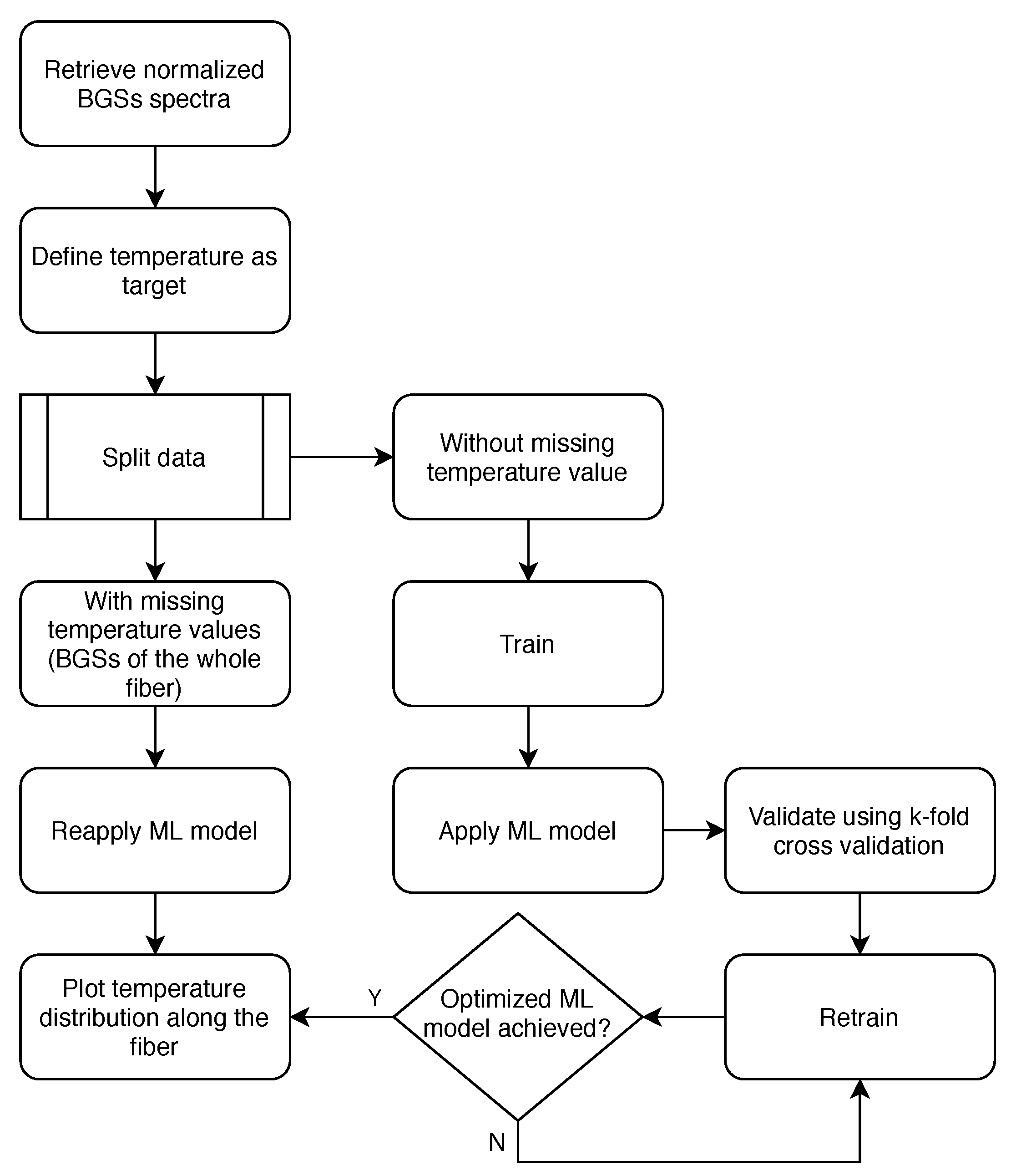
ML-Based Signal Processing

Five ML algorithms were selected in this study, namely the Deep Learning (DL), Random Forest (RF), Gradient Boosted Trees (GBT), Support Vector Machine (SVM), and Generalized Linear Model (GLM). DL is a multi-layer feed-forward form of ANN. DL and ANN have both been successfully employed for BOTDA previously [22,24,25,26]. DL or, also most commonly called as deep neural networks (DNN), is a ML model that consists of many parallel neurons and layers made to process the information from the input. The learning process is mimicking the function of the human brain. In each layer of DL, a set of features together with weights w i j were defined according to the importance of each feature. The accuracy of the prediction is used to determine how much correction of weight is needed. The process is repeated until it achieves the optimum accuracy. The layers after the input layer L 1 , can be expressed as
y j = f j ( w i j · x i θ j )
where y j is the output of the jth neuron in the current layer, f j is the activation function, w i j is the weight of the synapse connecting the ith neuron in the previous layer and the jth neuron in the current layer, x i is the output of the ith neuron in the previous layer, and finally θ j is a constant bias [36]. DL learned the features based on the training dataset and the architecture is well suited for two-dimensional (2D) data processing such as BGS-temperature dataset.
RF is a highly accurate nonlinear ML algorithm that is capable of handling noisy datasets. It is an ensemble of numerous decision trees (DT) that makes the prediction based on the combined models. Although it is usually outperformed by other ML models, RF is easy to apply, interpret, and understand. The key is to have low correlations or entirely uncorrelated between individual trees. RF uses the bagging and feature randomness technique in order to create variation from one tree to another. For BOTDA, the frequencies of the BGS are used as the feature in RF and the splitting nodes are based on the label, which is the temperatures.
GBT, on the other hand, is also an ensemble of regression or classification tree models. The boosting method is usually used for nonlinear regression to improve tree accuracy. However, there will be a decrease in processing speed as GBT increases its efficiency [37]. Additionally, GBT is less robust to noisy data due to over-fitting. The main difference between RF and GBT is that RF computes the average for every result at the end of the process as it grows trees in parallel, whereas GBT calculates the results after each step of growing trees sequentially. As GBT constructs one tree at a time, each new tree is an improved version of the previous tree. However, the feature and label for GBT is similar to RF for BOTDA data processing.
SVM finds the most significant margin between the points of different classes while creating an optimal hyper-plane. Predictions are made based on the optimal hyper-plane and support vectors of the SVM. The optimal hyper-plane can be expressed as
y ( X ) = W T X + b
where W is the norm of weight vector of the hyper-plane and b is the bias or the interception value [33]. W and b can be obtained from training samples and they controlled the margin width of SVM. This ML algorithm was implemented in BOTDA because of its accuracy and unlikeliness to overfit the data, as reported by Wu et al. [33]. The hyper-plane of SVM separates the temperature classes in BOTDA based on the BGSs. However, because the algorithm uses more than two classes, the processing time will gradually increase accordingly.
GLM is an extension of the general linear regression model introduced by Nelder et al. [38], which produces a response that is based on the maximum likelihood of the training parameters. The GLM calculates the mean of data that could be made up of Poisson, Lorentzian, normal, exponential, and a few other distributions to the linear predictor through link function. It uses the iteratively re-weighted least square technique onto the belonging distribution family to make maximum likelihood predictions. There are three main components in GLM; random component, systematic component, and link function. The random component is the distribution type of data (which is the Lorentzian distribution), whereas the systematic component for this study is given by
η i = β 0 + β 1 X i 1 + β 2 X i 2 + + β k X i k
where β are the estimated coefficients and X are the independent variable. The link function links the other two components together while using a linear predictor, given by
g ( μ i ) = η i = β 0 + β 1 X i 1 + β 2 X i 2 + + β k X i k
where μ i is the expected value of the response or also known as the dependent variable [38].
In this paper, these selected models were implemented using the RapidMiner tool [39] according to the process flow that was depicted in Figure 1. First, the BGS of each location was retrieved using an experimental setup discussed in the next section. Then the target value, which is the temperature value within the intended measurement range, was paired with the BGS, creating a dataset that has BGS-temperature pairs. This dataset was used to train the chosen ML algorithm. The regularization and optimization method were also adopted in the training phase to avoid overfitting. Subsequently, the dataset containing only the noisy BGSs, i.e., without pairing with temperature was used as test data for temperature prediction. The conventional LCF method was also calculated and used as a benchmark in order to study the efficacy of the selected ML algorithms.
To achieve an optimized model, the dataset was first tested using the k-fold cross validation method. The K-fold cross validation method is a prevalent and unbiased method used to evaluate ML model. In this method, the data were randomly split into k number of groups. Some of the groups were held out for testing later, whereas the remaining groups were used for training. Subsequently, the knowledge gained from the k-fold cross validation was utilized to retrain the model until an optimized model was achieved. Lastly, raw BGSs were fed into the optimized ML model, and the accuracy of each model’s prediction was evaluated.

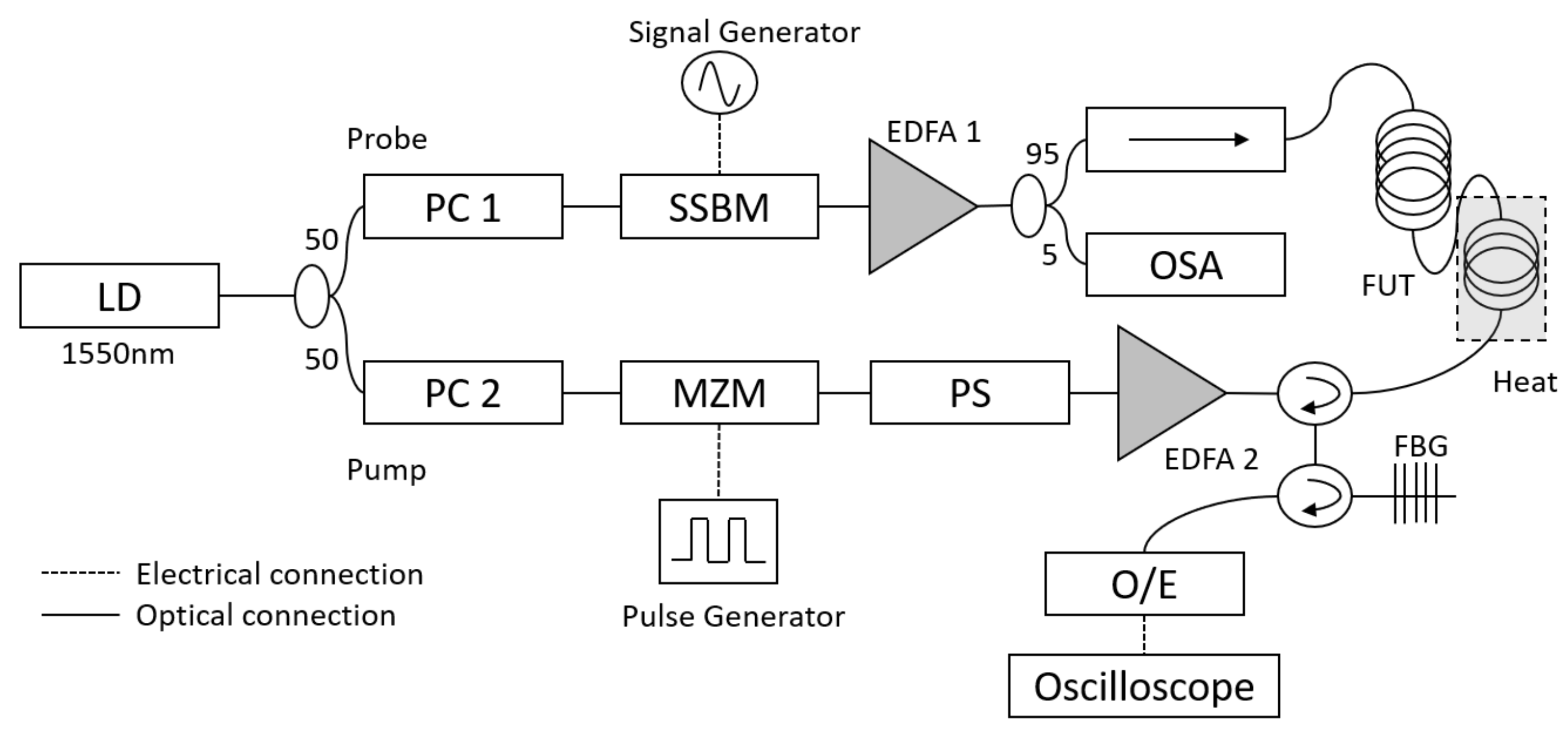
2. Experimental Setup

Figure 2 depicts the BOTDA experimental setup. A distributed feedback laser producing continuous wave (CW) light at 1552.92 nm and output power of 8 dBm was used as the light source. The CW light was then split into probe and pump signal by a 3 dB coupler. The probe arm (top part of the figure) consists of signal generator, single side-band modulator (SSBM), and erbium-doped fiber amplifier (EDFA 1). The pump arm (bottom part of the figure) consisted of a pulse generator, Mach-Zehnder modulator (MZM), polarization scrambler (PS), and another amplifier, EDFA 2.
The CW light in the probe arm was frequency modulated by the SSBM by carefully adjusting three DC-voltage power supplies to the modulator to produce probe light with downshifted frequency. The radio frequency signal generator controlled the amount of the frequency supplied to the SSBM. In order to construct the BGS, the frequency was swept between the range of 10.765 to 10.935 GHz. The frequency modulated signal was then launched into one end of the fiber under test (FUT) after being amplified to 0 dBm by EDFA 1. In the pump arm, the CW light was modulated by the MZM in order to generate an optical pulse via intensity modulation scheme. The duration of the electrical pulse supplied from the pulse generator (pulse generator clock speed: 250 MSa/s) was set to 20 ns, which corresponds to 2 m spatial resolution. The MZM having extinction ratio (ER) of around 25 dB, was biased at its minimum transmission point by a DC-voltage power supply for the intensity modulation process. Subsequently, the polarization state of the optical pulse from the MZM output was scrambled to reduce polarization induced noise. The optical pulse was amplified by EDFA 2 to approximately 25 dBm before being injected into the other end of the FUT. The measured SBS signal was filtered by a fiber Bragg grating (FBG), converted to an electrical signal by a 1 GHz bandwidth DC-coupled optical-to-electrical converter (O/E) and then digitized by an oscilloscope (bandwidth: 500 MHz, sampling rate 2.5 Gbps) at 5000 times averaging. The FUT used was a standard telecom grade single-mode fiber with a total length of around 1.26 km. A short section of about 8 m near the end of the FUT (at the probe input side) was placed on a hot plate where the temperature was set from 45 ° C to 85 ° C with 10 ° C increment. A thermocouple was used to continuously measure and monitor the temperature stability of the hot plate throughout the experiment. The recorded data were then ready to be deployed in the proposed algorithm.

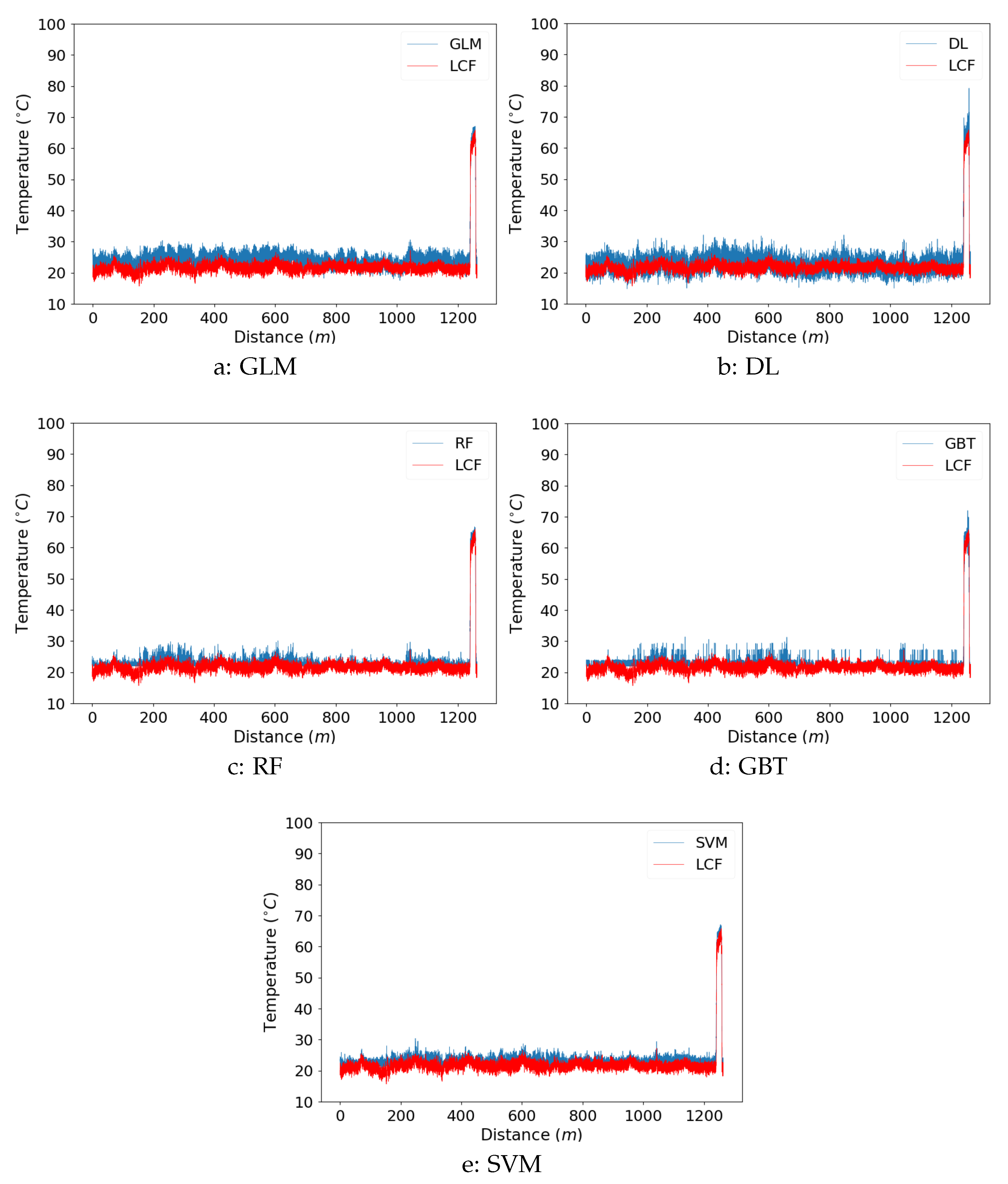
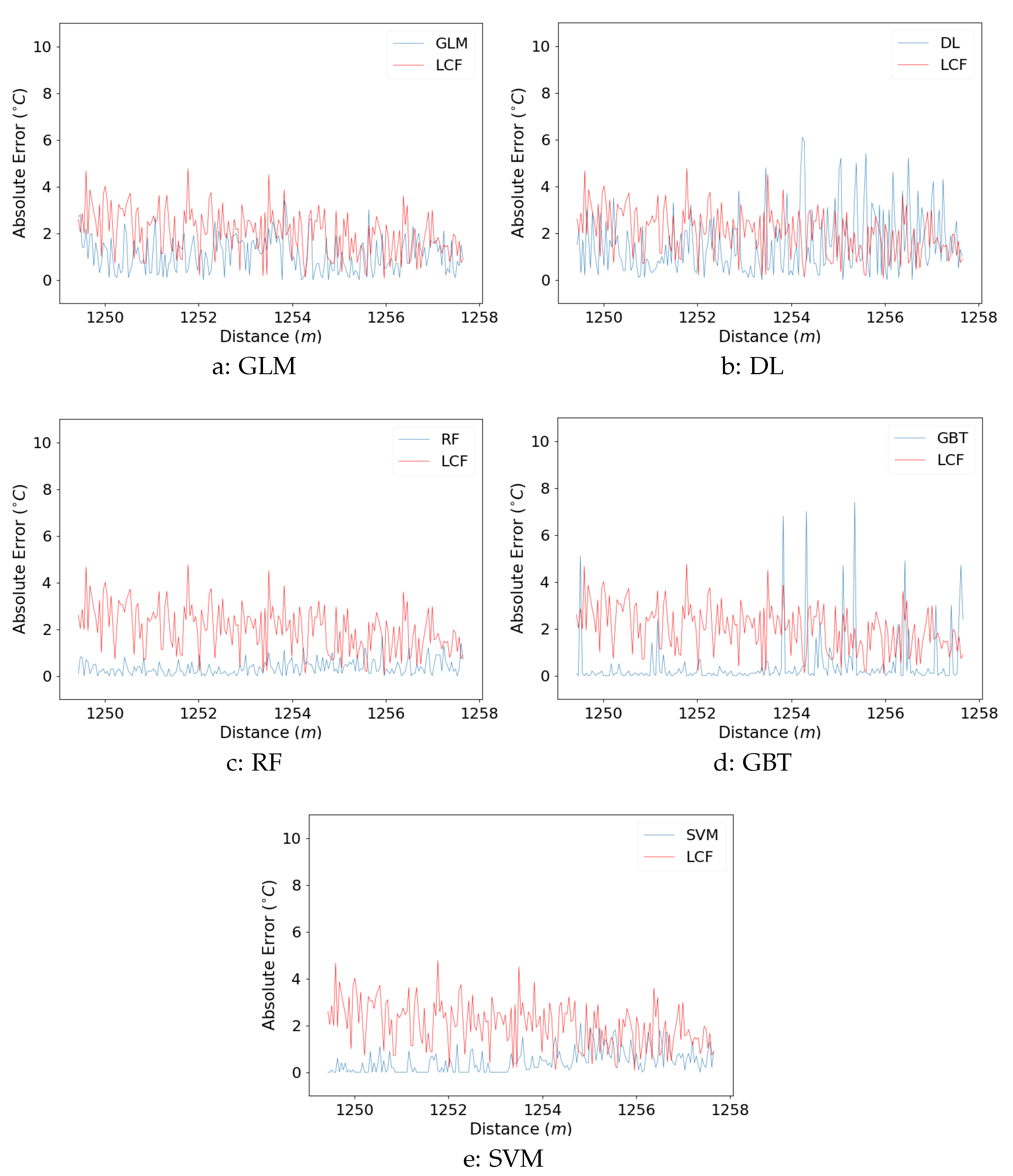
3. Results and Discussions

Conventionally, BGS along the FUT was constructed using the LCF method. From there, the central frequency of the BGS, i.e., the BFS can be determined to estimate the strain or temperature. The conventional LCF method that was used in this paper was based on the Levenberg-Marquardt algorithm (LMA), and was calculated by using the Python lmfit module [40]. This LMA-based LCF program also supports optimization method. It calculated the structure factor, convoluted with the instrumental resolution, and finally computed the optimal parameters by calculating the least square. As a representative, Figure 3 illustrates the acquired noisy BGS fitted with the conventional LCF method. It should be noted that, in this calculation, the signal amplitude of the BGS was normalized to unity.
The time that is required to construct the BGS, and eventually estimate the BFS depends on the frequency sweeping step, fiber length and the spatial resolution. However, with the help of ML modeling, the measurement time can be reduced to the extent of eliminating the need to determine the BFS and directly predicting the temperature distribution along the fiber from constructed BGS. In this work, the dataset for ML model training consists of 100 experimentally collected BGSs at every temperature setting. The ML model was trained and optimized before prediction for every spatial point along the fiber, as described in the previous section.
The performance of the proposed architecture was evaluated by comparing the result from k-fold cross validation for all five ML algorithms. In this case, the initial training dataset was randomly split, where 60% of the data were assigned as training subset while the remaining 40% as testing subset. Figure 4 shows the test result of the temperature prediction of all proposed ML models.
True-value regression analysis is the best form of data visualization for understanding the efficacy of the selected ML models. For an ideal ML model, the points should be as close as possible to the regress diagonal line, R. From Figure 4, the R values for GLM (0.9923), RF (0.9978), and SVM (0.9969) were the closest to the ideal value among all five models. It means that GLM, RF, and SVM would make a better prediction when compared to other methods. On the other hand, the R value for DL and GBT was 0.9752 and 0.9813, respectively, which was slightly lower than the others. This was due to the prediction made by both methods was scattered away from the regression line. Even though the R values for both methods were slightly low, they could still make the temperature prediction but with less accuracy. In addition, for comparison, we also analyzed the true vs. predicted temperature result for the conventional LCF method. It was found that the R value for LCF (0.9872) appeared to be slightly better than DL and GBT.
In order to further evaluate the ML models, they were tested with BGS distribution from the whole FUT length. Figure 5 shows the temperature distribution along the FUT predicted by all five ML models in comparison with that obtained by the conventional LCF method (in red). The normalized raw BGS datasets of the whole FUT were used as ML model’s input to directly extract the temperature distribution without obtaining the BFS as typically deployed in the conventional LCF method. It is also worth noting that, for all five ML algorithms, the spatial resolution is still retained, confirming the correct deployment of the ML algorithm in BOTDA sensor. The spatial resolution measured at the falling edge of the heated section was found to be around 2 m, which is consistent with the 20 ns of pulse duration used in the experiment. The measurement precision of predicted temperature by all five ML models were also evaluated by calculating the standard deviation. The temperature measurement precision for GLM was 1.59 ° C, DL was 1.98 ° C, RF was 1.05 ° C, GBT was 1.05 ° C, and SVM was 1.08 ° C. The temperature measurement precision for the conventional LCF was found to be around 1.22 ° C, which is only slightly better than that of the GLM and DL models. Therefore, generally speaking, the analyzed ML models were found to be comparable to one another.
For further evaluation, the absolute error distribution at a specific location of the heated section was calculated by comparing the temperature predicted by each ML model and conventional LCF method with the thermocouple reading, which is regarded as true temperature of 65 ° C. The difference between the two measurements defines absolute error. The results are shown in Figure 6. From the figure, GLM (Figure 6a), RF (Figure 6c) and SVM (Figure 6e) show lower absolute error compared to the conventional LCF method. However, the absolute error distribution for the DL (Figure 6b) and GBT (Figure 6d) are much more inconsistent. However, it is also important to note that, for both DL and GBT cases, the inconsistency in absolute error does not truly represent the actual performance of the algorithm, due to the insufficient number of data collected for training dataset. To improve the performance of both models, at the training stage, smaller temperature step size dataset, such as 1 ° C temperature step, could be used. However, this would require longer training time and longer processing time as the structure becomes much more complex.
To obtain a deeper insight on the effectiveness of the ML models, the prediction accuracy was then calculated from the root mean square error (RMSE) formula at the heated section of the FUT. Again, the error was also calculated by taking the thermocouple reading as the true temperature (65 ° C). Overall, the results indicated that the RMSE for all of the five ML models was lower than that of the conventional LCF method. The RF showed the lowest RMSE of around 0.48 ° C, followed by SVM (0.69 ° C), GBT (1.25 ° C) and GLM 1.32 ° C. DL produced the largest RMSE of around (2.03 ° C), but still lower than the conventional LCF (2.25 ° C).
Finally, the processing time for all of the ML methods to retrieve a temperature distribution for the whole length of FUT that consisted of 30,735 spectra were compared. In general, all of the ML models deployed in this experiment provided faster signal processing time than the conventional LCF, which took around 655 s. GLM recorded the fastest processing time of only 1 s. This was followed by DL, which took 3 s, but with slightly larger measurement precision than the LCF method and a comparable prediction accuracy. SVM required about 21 s to process the signal, followed by RF of around 31 s. GBT required the longest processing time, which was around 184 s; still 3.5 times faster than the conventional LCF method. The reason behind this is because, as GBT increased its prediction accuracy, the speed will gradually decrease.
To summarize, after the 30,735 BGS spectra are obtained from BOTDA measurement, the LCF method required curve fitting onto the individual BGS in order to find the corresponding center frequency (BFS) before translating it into temperature. On the other hand, for ML models, the step of retrieving BFS can be entirely discarded and thus significantly reducing the total processing time. Once the ML models are trained, the measured BGS spectra can be directly inputted into the model in order to obtain the temperature prediction.
The summary of the performance of all ML models is as shown in Table 1. In terms of measurement precision, RF and GBT gave the best result. However, the measurement precision for all other ML models is comparable to the conventional LCF method. In terms of prediction accuracy, RF is the best performing model, and DL is the worst. Both temperature prediction accuracy and measurement precision are a measure of errors, which however are slightly different. Temperature measurement precision refers to the statistical variability of the data. It reflects on how reproducible measurements are even if the points are far away from the actual value. In contrast, temperature prediction accuracy reflects on the analysis of the predicted result when compared to the actual value. Measurement precision is independent of prediction accuracy and, therefore, it is possible to have high measurement precision but less prediction accuracy, like GBT.
In terms of the processing time, GLM offered the fastest processing time. Even though RF and SVM are not the fastest, both of the models have high measurement precision and prediction accuracy. In addition to that, the processing time for RF and SVM are still lower than 1 min. It can be concluded that based on these findings, GLM, RF, and SVM showed the best alternative method to process BGS distribution for the BOTDA technique. This can be beneficial for real-time monitoring applications in various fields. For an application requiring fast analysis, GLM may be the best choice, since it is the quickest model to generate predicted outcome. Additionally, we had previously demonstrated that GLM has better prediction accuracy than LCF method even at larger frequency scanning step and lower SNR [34]. At the same time, RF and SVM may be suitable for a system requiring higher measurement precision and prediction accuracy, but it can tolerate slightly longer processing times. In short, depending on the requirement stipulated by a particular application of choice, some models may have advantages over the other.

4. Conclusions

A comparative analysis of five ML models for fast and accurate temperature information prediction from the BOTDA fiber sensor was successfully demonstrated. The ML models analyzed in this study have significantly shortened the BOTDA signal processing time by discarding the BFS retrieving process when compared to the conventional LCF method and, at the same time, retaining high- temperature prediction accuracy, temperature measurement precision and spatial resolution. In the training phase, the BGS and temperature pairs dataset were collected experimentally according to the BFS-temperature coefficient of the fiber before being fed into the model. The models were then retrained to ensure that the pattern of the BGS and temperature pairing information were optimized. Finally, the optimized ML model was applied with noisy raw BGS collected along the fiber to determine the temperature distribution. In terms of the signal processing time, all of the analyzed ML algorithms have significantly reduced the processing time to be between 3.5 and 655 times faster than the conventional LCF method. While DL method recorded the comparable temperature measurement precision- and temperature prediction accuracy performances with that of the conventional LCF method, the GLM, RF, and SVM methods showed even better results. The analyzed ML models can potentially replace the conventional processing technique, to become the attractive solutions for BOTDA fiber sensor technology, especially for real time and high measurement performance applications.

Author Contributions

Conceptualization, N.D.N., M.S.D.Z. and F.A.; methodology, N.D.N.; software, N.D.N.; data curation, N.D.N.; writing—original draft preparation, N.D.N.; writing—review and editing, M.S.D.Z and F.A.; supervision, M.S.D.Z. and F.A. All authors have read and agreed to the published version of the manuscript.

Funding

This research was funded by Fundamental Research Grant Scheme (FRGS), grant number FRGS/1/2019/TK04/UKM/02/2, Geran Universiti Penyelidikan (GUP-2019-024) from Universiti Kebangsaan Malaysia (UKM), UNITEN R&D Sdn. Bhd. and TNB Research Sdn. Bhd. consultancy project number U-SN-CR-17-01.

Conflicts of Interest

The authors declare no conflict of interest. The funders had no role in the design of the study; in the collection, analyses, or interpretation of data; in the writing of the manuscript, or in the decision to publish the results.

References

  1. Li, C.; Li, Y. Fitting of Brillouin Spectrum Based on LabVIEW. In Proceedings of the 2009 5th International Conference on Wireless Communications, Networking and Mobile Computing, Beijing, China, 24–26 September 2009; pp. 1–4. [Google Scholar] [CrossRef]
  2. Galindez-Jamioy, C.A.; López-Higuera, J.M. Brillouin distributed fiber sensors: An overview and applications. J. Sens. 2012, 2012, 204121. [Google Scholar] [CrossRef] [Green Version]
  3. Bao, X.; Chen, L. Recent Progress in Distributed Fiber Optic Sensors. Sensors 2012, 12, 8601–8639. [Google Scholar] [CrossRef] [PubMed] [Green Version]
  4. Motil, A.; Bergman, A.; Tur, M. [INVITED] State of the art of Brillouin fiber-optic distributed sensing. Opt. Laser Technol. 2016, 78, 81–103. [Google Scholar] [CrossRef]
  5. Zan, M.S.D.B.; Horiguchi, T. A dual golay complementary pair of sequences for improving the performance of phase-shift pulse BOTDA fiber sensor. J. Lightwave Technol. 2012, 30, 3338–3356. [Google Scholar] [CrossRef]
  6. Zan, M.S.D.B.; Tsumuraya, T.; Horiguchi, T. The use of Walsh code in modulating the pump light of high spatial resolution phase-shift-pulse Brillouin optical time domain analysis with non-return-to-zero pulses. Meas. Sci. Technol. 2013, 24, 9. [Google Scholar] [CrossRef]
  7. Horiguchi, T.; Tateda, M. BOTDA-nondestructive measurement of single-mode optical fiber attenuation characteristics using Brillouin interaction: Theory. J. Lightwave Technol. 1989, 7, 1170–1176. [Google Scholar] [CrossRef]
  8. Horiguchi, T.; Shimizu, K.; Kurashima, T.; Tateda, M.; Koyamada, Y. Development of a distributed sensing technique using Brillouin scattering. J. Lightwave Technol. 1995, 13, 1296–1302. [Google Scholar] [CrossRef]
  9. Nikles, M.; Thevenaz, L.; Robert, P.A. Measurement of the distributed-Brillouingain spectrum in optical fibers by using a single laser source. In Proceedings of the Conference on Optical Fiber Communication, San Jose, CA, USA, 20 February 1994; OSA: Washington, DC, USA, 1994; p. WF1. [Google Scholar] [CrossRef] [Green Version]
  10. Kurashima, T.; Horiguchi, T.; Tateda, M. Distributed-temperature sensing using stimulated Brillouin scattering in optical silica fibers. Opt. Lett. 1990, 15, 1038. [Google Scholar] [CrossRef]
  11. Horiguchi, T.; Kurashima, T.; Koyamada, Y. Measurement of temperature and strain distribution by Brillouin frequency shift in silica optical fibers. In Distributed and Multiplexed Fiber Optic Sensors II; Dakin, J.P., Kersey, A.D., Eds.; International Society for Optics and Photonics, SPIE: Bellingham, WA, USA, 1993; Volume 1797, pp. 2–13. [Google Scholar] [CrossRef]
  12. Ukil, A.; Braendle, H.; Krippner, P. Distributed temperature sensing: Review of technology and applications. IEEE Sens. J. 2012, 12, 885–892. [Google Scholar] [CrossRef] [Green Version]
  13. Soto, M.A.; Thévenaz, L. Modeling and evaluating the performance of Brillouin distributed optical fiber sensors. Opt. Express 2013, 21, 31347. [Google Scholar] [CrossRef]
  14. Zhang, C.; Yang, Y.; Li, A. Application of Levenberg-Marquardt algorithm in the Brillouin spectrum fitting. In Proceedings of the Seventh International Symposium on Instrumentation and Control Technology: Optoelectronic Technology and Instruments, Control Theory and Automation, and Space Exploration, Beijing, China, 10–13 October 2008; Fang, J., Wang, Z., Eds.; International Society for Optics and Photonics, SPIE: Bellingham, WA, USA, 2008; Volume 7129, pp. 443–449. [Google Scholar] [CrossRef]
  15. Farahani, M.A.; Castillo-Guerra, E.; Colpitts, B.G. Accurate estimation of Brillouin frequency shift in Brillouin optical time domain analysis sensors using cross correlation. Opt. Lett. 2011, 36, 4275. [Google Scholar] [CrossRef]
  16. Farahani, M.A.; Castillo-Guerra, E.; Colpitts, B.G. A detailed evaluation of the correlation-based method used for estimation of the Brillouin frequency shift in BOTDA sensors. IEEE Sens. J. 2013, 13, 4589–4598. [Google Scholar] [CrossRef]
  17. Qasem, A.; Abdullah, S.N.H.S.; Sahran, S.; Wook, T.S.M.T.; Hussain, R.I.; Abdullah, N.; Ismail, F. Breast cancer mass localization based on machine learning. In Proceedings of the 2014 IEEE 10th International Colloquium on Signal Processing and Its Applications, Kuala Lumpur, Malaysia, 7–9 March 2014; pp. 31–36. [Google Scholar] [CrossRef]
  18. Alshalabi, H.; Tiun, S.; Omar, N.; Albared, M. Experiments on the Use of Feature Selection and Machine Learning Methods in Automatic Malay Text Categorization. Procedia Technol. 2013, 11, 748–754. [Google Scholar] [CrossRef] [Green Version]
  19. Alsaffar, A.; Omar, N. Study on feature selection and machine learning algorithms for Malay sentiment classification. In Proceedings of the 6th International Conference on Information Technology and Multimedia at UNITEN: Cultivating Creativity and Enabling Technology Through the Internet of Things, (ICIMU 2014), Putrajaya, Malaysia, 18–20 November 2015; pp. 270–275. [Google Scholar] [CrossRef]
  20. Umar, I.K.; Gokcekus, H. Modeling Severity of Road Traffic Accident in Nigeria using Artificial Neural Network. J. Kejuruter. 2019, 31, 221–227. [Google Scholar]
  21. Sani, M.M.; Ishak, K.A.; Samad, S.A. Evaluation of face recognition system using Support Vector Machine. In Proceedings of the 2009 IEEE Student Conference on Research and Development (SCOReD), Serdang, Malaysia, 16–18 November 2009; pp. 139–141. [Google Scholar] [CrossRef]
  22. Azad, A.K.; Wang, L.; Guo, N.; Tam, H.Y.; Lu, C. Signal processing using artificial neural network for BOTDA sensor system. Opt. Express 2016, 24, 6769. [Google Scholar] [CrossRef]
  23. Li, Y.; Wang, J. Optimized neural network for temperature extraction from Brillouin scattering spectra. Opt. Fiber Technol. 2020. [Google Scholar] [CrossRef]
  24. Ruiz-Lombera, R.; Serrano, J.M.; Lopez-Higuera, J.M. Automatic strain detection in a Brillouin Optical Time Domain sensor using Principal Component Analysis and Artificial Neural Networks. In Proceedings of the SENSORS, 2014 IEEE, Valencia, Spain, 2–5 November 2014; pp. 1539–1542. [Google Scholar] [CrossRef]
  25. Ruiz-Lombera, R.; Piccolo, A.; Rodriguez-Cobo, L.; Lopez-Higuera, J.M.; Mirapeix, J. Feasibility study of strain and temperature discrimination in a BOTDA system via artificial neural networks. In Proceedings of the 2017 25th Optical Fiber Sensors Conference (OFS), Jeju, Korea, 24–28 April 2017; pp. 1–4. [Google Scholar] [CrossRef] [Green Version]
  26. Ruiz-Lombera, R.; Fuentes, A.; Rodriguez-Cobo, L.; Lopez-Higuera, J.M.; Mirapeix, J. Simultaneous Temperature and Strain Discrimination in a Conventional BOTDA via Artificial Neural Networks. J. Lightwave Technol. 2018, 36, 2114–2121. [Google Scholar] [CrossRef] [Green Version]
  27. Wang, J.; Li, Y.; Liao, J. Temperature extraction for Brillouin optical fiber sensing system based on extreme learning machine. Opt. Commun. 2019, 453, 124418. [Google Scholar] [CrossRef]
  28. Azad, A.; Wang, L.; Guo, N.; Lu, C.; Tam, H. Temperature sensing in BOTDA system by using artificial neural network. Electron. Lett. 2015, 51, 1578–1580. [Google Scholar] [CrossRef]
  29. Azad, A.K.; Wang, L.; Guo, N.; Lu, C.; Tam, H.Y. Temperature profile extraction using artificial neural network in BOTDA sensor system. In Proceedings of the 2015 Opto-Electronics and Communications Conference (OECC), Shanghai, China, 28 June–2 July 2015; pp. 1–3. [Google Scholar] [CrossRef]
  30. Azad, A.K.; Khan, F.N.; Alarashi, W.H.; Guo, N.; Lau, A.P.T.; Lu, C. Temperature extraction in Brillouin optical time-domain analysis sensors using principal component analysis based pattern recognition. Opt. Express 2017, 25, 16534–16549. [Google Scholar] [CrossRef]
  31. Wang, B.; Wang, L.; Guo, N.; Zhao, Z.; Yu, C.; Lu, C. Deep neural networks assisted BOTDA for simultaneous temperature and strain measurement with enhanced accuracy. Opt. Express 2019, 27, 2530–2543. [Google Scholar] [CrossRef]
  32. Chang, Y.; Wu, H.; Zhao, C.; Shen, L.; Fu, S.; Tang, M. Distributed Brillouin frequency shift extraction via a convolutional neural network. Photonics Res. 2020, 8, 690–697. [Google Scholar] [CrossRef]
  33. Wu, H.; Wang, L.; Zhao, Z.; Shu, C.; Lu, C. Support Vector Machine based Differential Pulse-width Pair Brillouin Optical Time Domain Analyzer. IEEE Photonics J. 2018, 10, 6802911. [Google Scholar] [CrossRef]
  34. Nordin, N.D.; Zan, M.S.D.; Abdullah, F. Generalized linear model for enhancing the temperature measurement performance in Brillouin optical time domain analysis fiber sensor. Opt. Fiber Technol. 2020, 58, 102298. [Google Scholar] [CrossRef]
  35. Pan, Q.; Huang, X.; Min, R.; Liu, W. Fast frame synchronization design and FPGA implementation in SF-BOTDA. Photonics 2020, 7, 17. [Google Scholar] [CrossRef] [Green Version]
  36. Wang, L.; Wang, B.; Jin, C.; Guo, N.; Yu, C.; Lu, C. Brillouin optical time domain analyzer enhanced by artificial/deep neural networks. In Proceedings of the 2017 16th International Conference on Optical Communications and Networks (ICOCN), Wuzhen, China, 7–10 August 2017; pp. 1–3. [Google Scholar] [CrossRef]
  37. Brink, H.; Richards, J.W.; Fetherolf, M. Real-World Machine Learning; Manning Publications: Shelter Island, NY, USA, 2016. [Google Scholar]
  38. Hastie, T.J.; Pregibon, D. Generalized Linear Models. In Statistical Models in S; Hastie, T.J., Ed.; Taylor & Francis: New York, NY, USA, 2017; Chapter 6; pp. 193–246. [Google Scholar]
  39. Mierswa, I.; Wurst, M.; Klinkenberg, R.; Scholz, M.; Euler, T. YALE: Rapid Prototyping for Complex Data Mining Tasks. In Proceedings of the 12th ACM SIGKDD International Conference on Knowledge Discovery and Data Mining (KDD’06), Philadelphia, PA, USA, 20–23 August 2006; ACM: New York, NY, USA, 2006; pp. 935–940. [Google Scholar] [CrossRef]
  40. Newville, M.; Stensitzki, T.; Allen, D.B.; Ingargiola, A. LMFIT: Non-Linear Least-Square Minimization and Curve-Fitting for Python. Available online: https://zenodo.org/record/11813#.X08GJIsRXIV (accessed on 2 September 2020).
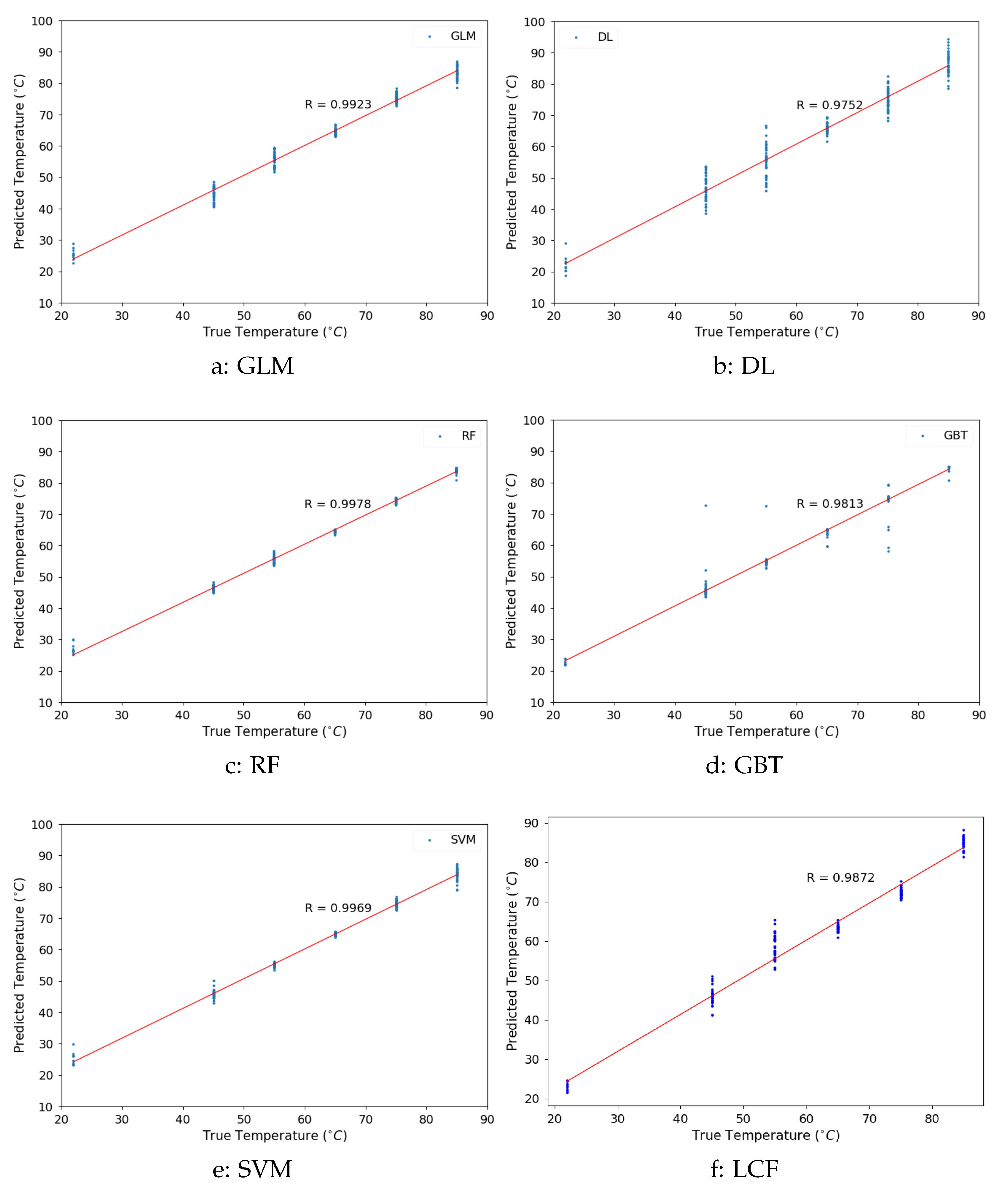
Figure 1. The flowchart in building an ML model.
Photonics 07 00079 g001
Figure 2. Experimental setup.
Photonics 07 00079 g002
Figure 3. Fitted Lorentzian curve fitting (LCF) method on a noisy Brillouin gain spectrum (BGS).
Photonics 07 00079 g003
Figure 4. True vs. predicted temperature results by using k-fold cross validation for ML models (ae) and by conventional LCF method (f).
Photonics 07 00079 g004
Figure 5. Temperature distribution along the fiber (65 ° C case).
Photonics 07 00079 g005
Figure 6. Absolute error at heated location (65 ° C case).
Photonics 07 00079 g006
Table 1. Summary of the model performance.
ParameterLCFGLMDLRFGBTSVM
Measurement Precision ( ° C )1.221.591.981.051.051.08
Prediction Accuracy ( ° C )2.251.322.030.481.250.69
Time (s)655133118421

