Neural Network DPD for Aggrandizing SM-VCSEL-SSMF-Based Radio over Fiber Link Performance


1
Department of Electronic Systems, Aalborg University, 9220 Aalborg Øst, Denmark
2
Faculty of Computer Engineering, Edge Hill University, Ormskirk L39 4QP, UK
3
Electrical Engineering Department, National University of Sciences and Technology (NUST), Islamabad 44000, Pakistan
4
Nokia Bell Labs, Murray Hill, NJ 07974-0636, USA
*
Author to whom correspondence should be addressed.
Photonics 2021, 8(1), 19; https://0-doi-org.brum.beds.ac.uk/10.3390/photonics8010019
Submission received: 22 December 2020
/
Revised: 5 January 2021
/
Accepted: 12 January 2021
/
Published: 14 January 2021
(This article belongs to the Special Issue Radio over Fiber)
Abstract
:This paper demonstrates an unprecedented novel neural network (NN)-based digital predistortion (DPD) solution to overcome the signal impairments and nonlinearities in Analog Optical fronthauls using radio over fiber (RoF) systems. DPD is realized with Volterra-based procedures that utilize indirect learning architecture (ILA) and direct learning architecture (DLA) that becomes quite complex. The proposed method using NNs evades issues associated with ILA and utilizes an NN to first model the RoF link and then trains an NN-based predistorter by backpropagating through the RoF NN model. Furthermore, the experimental evaluation is carried out for Long Term Evolution 20 MHz 256 quadraturre amplitude modulation (QAM) modulation signal using an 850 nm Single Mode VCSEL and Standard Single Mode Fiber to establish a comparison between the NN-based RoF link and Volterra-based Memory Polynomial and Generalized Memory Polynomial using ILA. The efficacy of the DPD is examined by reporting the Adjacent Channel Power Ratio and Error Vector Magnitude. The experimental findings imply that NN-DPD convincingly learns the RoF nonlinearities which may not suit a Volterra-based model, and hence may offer a favorable trade-off in terms of computational overhead and DPD performance.
1. Introduction
The fifth generation, commonly known as 5G, of mobile networks is envisioned to uplift capacity, efficiency, capacity and latency [1]. Since 5G technology should address all application scenarios, third generation partnership project (3GPP) set the frequency limits in the 5G new radio (NR) standard, namely, frequency range 1 (FR1: 0.4–7.1 GHz range) and frequency range 2 (FR2: 24–52.6 GHz) [2].
Furthermore, due to an exponential increase in base stations (BS), the radio access network (RAN) has to be primarily centralized. A fronthaul (FH) is utilized for connecting baseband units (BBUs) and Remote Radio units (RRUs). The Centralized/Cloud Radio Access Network (C-RAN) primarily simplifies the network traffic and enhances the scalability (see Figure 1).
In this context, microwave photonics techniques such as radio over fiber (RoF) systems are the backbone of fed analog or digital signals in optical FH using RoF systems. RoF systems provide cost effective and beneficial solutions by escalating the extent of wireless links for short, medium and long reach networks [3,4]. Other than their significant highlights, such as impunity to electromagnetic interventions, low-loss and broad bandwidth, RoF links are liable to nonlinearities which can be solved using linearization methods [5,6,7]. RoF has many forms, such as analog radio over fiber (A-RoF) [1,3,4], digital radio over fiber (D-RoF) [8,9] and Sigma Delta radio over fiber (S-DRoF) [10,11,12] systems. However, A-RoF suffers from nonlinearities, still due to the complexity of the other realizations and advantages in A-RoF that include simplicity, cost effectiveness and already widely spread legacy infrastructure, making it a better choice as compared to more efficient and costly solutions, such as D-RoF and S-DRoF [12].
Analog fronthaul applications are limited due to the nonlinearities that arise due to microwave and optical parts. The amelioration of these nonlinearities has gained immense importance to increase the optical system capacity. Many nonlinearity mitigating techniques have been proposed in recent years to subdue these nonlinearities and improve the performance of such cost-effective systems [3,5,6,7,12,13,14,15,16,17,18,19]. However, these solutions have been questioned due to a limited bandwidth and need of feedbacking the output, which is an overlong process [5]. Similarly, for 5G networks, it would be strenuous to perform dynamic tracking while compensating the nonlinear channel response with broadband time varying data traffic from different RATs.
When we consider short range A-RoF links, the impact of impairments that arise due to concoction of fiber chromatic dispersion and laser frequency chirp is usually negligible [4,5]. However, still, the impact of signal impairments owing to the laser diode and photodiode is significant.
Similarly, these nonlinearities result in a rise of near channel interference and affect the quality of transmission. As explained in [6], similar to fifth generation (5G) and Long-Term Evolution (LTE) signals, Orthogonal Frequency Division Modulated (OFDM) signals are susceptible to distortions attributed to a high peak to average power ratio (PAPR) in their signal envelope [7]. These systems generate undesired spurious terms due to relatively stable causes such as nonlinear characteristic curves of lasers and possibly photodiodes. It is, therefore, necessary to reduce these spurious terms, to investigate optimal DPD techniques.
Moreover, in fiber-wireless integrated systems, the nonlinearities become serious when the analog fiber and wireless links are cascaded together [20]. They may arise due to the nonlinear laser transfer function [21,22], combined effect of laser chirp and fiber chromatic dispersion [23], fiber kerr nonlinearity [24] and various nonlinearities attributed to the microwave photonic link. The generation of inadmissible specious terms is due to nonlinear characteristics of lasers and perhaps photodiodes. Therefore, reducing these undesired terms can enhance performance.
Efficiently reducing these nonlinearities through linearization techniques has critical importance. In previous years, different linearization methods have been proposed [3,5,6,7,13,14,15,16,17,18]; however, digital predistortion (DPD) demonstrated itself as a successful technique in mollifying the impairments in RoF systems [15,16,17,18]. Traditional Volterra-based methods such as Memory Polynomial (MP) and Generalized Memory Polynomial (GMP) were used successfully in [15,17,18], reducing the laser nonlinearities. Similarly, a comparison was shown in [6] where DPD based on Canonical Piecewise Linearization (CPWL) outperformed the traditional Volterra methods by reducing the nonlinearities. Although the performance can be passable, the computation complexity needed for such methods can be extremely high requiring hundreds of coefficients and exhaustive training [18]. Similarly, these methods require the output to come to the central office during the periodical training phase. If the RoF uplink is set for this purpose, the nonlinearities in this case should be compensated. This feedback mechanism adds extra complexity to the process of DPD [6].
In recent years, machine learning (ML) solutions have advanced significantly. Neural networks (NNs) are expected to learn any nonlinear function; therefore, it becomes trivial that NNs can be used for predistortion. NN-based DPD will be very meaningful if we are able to circumvent the bottle neck that was created regarding the complexity of DPD due to Volterra-based methods.
NNs were applied for DPD in Power Amplifiers (PA) [25] that rely on indirect learning architecture (ILA) for training the predistorter. The ILA that was initially designed for NNs [26] was applied to DPD for the first time in [27]. As it is well known that in an ILA, a postdistorter learns an inverse model followed by its usage as a predistorter, the learning of a postdistorter is dependent on the noise in the feedback signal [25,28].
A detailed study on ML utilization for RoF systems was discussed in [29,30,31,32]. Zibar et al. in [29] discussed general optical communications and optical networks in terms of ML solutions. Whilst some works on the application of machine learning techniques in radio over fiber systems and networks have been reviewed, due to the general scope, the reviews in this field are relatively brief and limited. Recently, in [30,31], machine learning techniques were surveyed that include NNs, k-means technique, the convolutional neural network (CNN) and the reinforcement learning category. It also highlights different application scenarios. Recently, a Support Vector Machine (SVM)-based ML method was used to mitigate nonlinearities in A-RoF systems [31,32]. However, it is a non-NN-based solution.
Inspired by the NNs work on PA and the known problems of Volterra-based predistortion using ILA, we, for the first time, propose to counter the nonlinearities in A-RoF for Single Mode VCSEL (SM-VCSEL) using a Standard Single Mode Fiber (SSMF)-based RoF system with a novel DPD method that exploits NNs by evading the ILA.
Our proposed methodology is based on the fact that, firstly, we should look for an ideal RoF input signal as it is unknown. Since this ideal RoF input signal is unknown, an NN-based predistorter cannot be trained immediately in the first step.
After this step, an NN-DPD model is cascaded with the NN-RoF model. The ideal output of RoF is now known; therefore, it is a straightforward procedure to evaluate the error of the cascaded network (NN-DPD and RoF model). This error can then be backpropagated through the NNs, consequently updating the DPD-NN. This DPD NN can then be cascaded with the actual RoF link.
The NN-based predistorter is advantageous, as it is flexible as compared to Volterra-based methods. We have seen in [16,17,18] that the GMP model often requires many coefficients adding extra complexity and overheads. Contrarily, in NN-based DPD, this issue does not exist, as it should be able to learn all of the effects causing the error function; therefore, explicit designing of all possible causes of distortion in a model is not required. For instance, as explained in [33], if we want to correct for IQ imbalance, a simple Volterra-based method is unable to correct it. This requires an additional methodology to be implemented in the predistorter that further increases the complexity of the system manifolds. By the nature of the fully connected NN, the NN can learn such impairments and correct them.
The significant contributions of this paper are listed as follows:
- A novel NN-based DPD algorithm is proposed for the linearization of RoF links.
- This NN-DPD method has been implemented with a new training method without the utilization of indirect learning architecture where a separate RoF-NN is used to first model the RoF link. Once modelled, by back propagating the error through RoF-NN, the DPD-NN is trained.
- The complexity of the proposed algorithms is estimated.
- For the first time, an experimental comparative study has been conducted where DPD-NN, DPD-MP and DPD-GMP are compared in terms of Adjacent Channel Power Ration (ACPR) and Error Vector Magnitude (EVM).
The remaining part of the paper is organized as follows. Firstly, we discuss the architecture of the NN to perform DPD covering model overview, model characteristics, design and NN training. Then, a Volterra method-based methodology is discussed, and its architecture is explained. This is followed by complexity considerations of NN and GMP. Then, the section discusses the experimental setup utilized followed by a discussion of future directions. Finally, conclusions are presented.
2. Neural Network-Based DPD Architecture
The proposed NN DPD system is cascaded with the RoF link so that the overall result of this system will be a linear system. The proposed method is shown in Figure 2. It must be noted that training an NN requires training data, whereas the ideal NN output is not known. Since the ideal RoF output is known, an RoF NN model is trained to emulate the RoF link. By doing this, we can backpropagate through the RoF NN model to update the parameters in the NN DPD.
Consider that an RoF link with transfer function (discrete time domain) will have output signal . Let us consider a complex baseband signal that must be sent through an RoF link. The goal of DPD is to calculate the inverse transfer function of the RoF expressed as , which will then have an output of . The simplified version can be expressed as:
while
This means that NN is used to find for predistortion. Since a training input and output sequence are required for NN training, however, the ideal is not known and, therefore, a direct training to establish an NN for DPD is unachievable. We must note that ILA can be used for this identification; however, we would like to evaluate the other option for performance measurements (see Figure 3).
So, first of all, the second NN model is used to model the RoF link. Considering and as input and output data for the generic RoF link, training is carried out with the regression-based NN for these data, causing the NN to learn and identify the approximated transfer function . Once the RoF NN model is established, the weights of the NN RoF model are fixed and it is connected to NN DPD. Consequently, the actual input and output training data are used to determine the error via loss function. This is then backpropagated via to train .
2.1. NN Model Characteristics and Design
As far as structure of the NN is concerned, there are two NNs proposed and used in this project whose description is given below:
- A DPD NN is utilized to predistort the “real” RoF link.
- An RoF NN model is required to train the DPD NN.
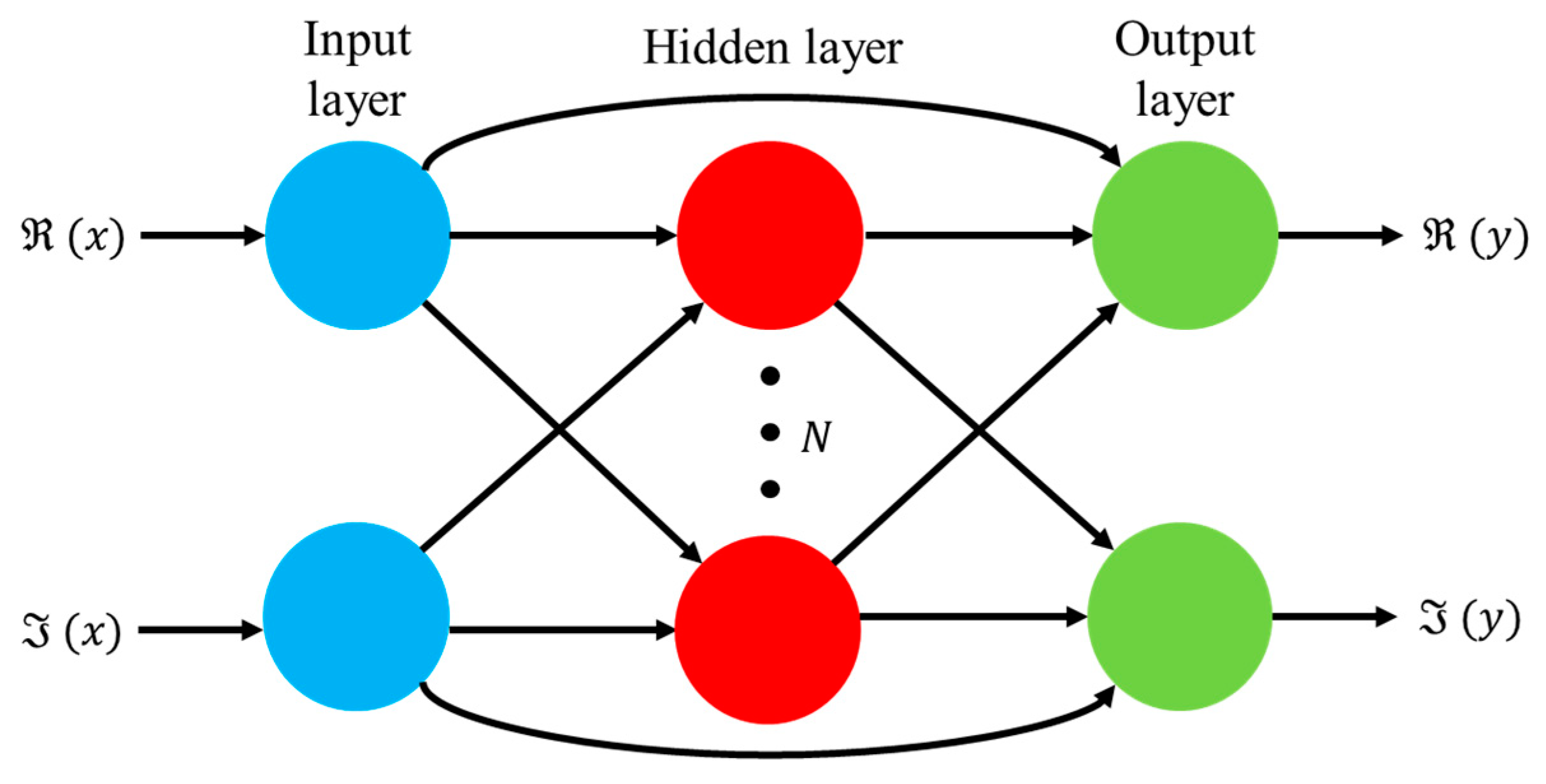
The NN utilized in this work was a feedforward fully connected (FC) NN. The FC-NN contained hidden layers and neurons per hidden layer. The schematic of the structure utilized in NN is shown in Figure 4. Considering the complex baseband signal, the NNs have two inputs and two outputs, i.e., one for the real and the other for the imaginary part. For the hidden layer (one layer at least), ReLu was used. There are different sets of nonlinear activations that can be applied in the hidden layers; however, a rectified linear unit (ReLu) was chosen due to its lower complexity.
The output for the first hidden layer is expressed below in (3):
Here, represents the first hidden output layer, represents the nonlinear activation function and and represent the weight and bias for the 1st output layer in NN.
Similarly, a general output for the ith layer can be expressed as:
where The final output after hidden layers N for the network is expressed in (5):
2.2. C. NN Training
The training algorithm for the NN DPD system is shown below (Algorithm 1). The mean square error is chosen as the loss function. ADAM is chosen as a standard optimizer. The update of weights is performed via backpropagation. In order to improve performance, the process can be repeated further for fine tuning of parameters for a total of Z iterations.
As explained earlier, the input and output data of “actual” RoF link are used to train NN that models the RoF link behavior. Once the model is obtained, a second DPD NN is connected to the RoF NN model. Once this training converges, the DPD NN is connected with the “real” RoF link to predistort it and conduct the parametric evaluation.
It is assumed that the training can be implied in an offline manner. Once the model is converged (learned), the model can run without any significant updates. However, occasional retraining may be required in some scenarios such as variation in temperature and length.
| Algorithm 1. Training Performed |
| ← for i Z do ← : // RoF Transmission ← Train on , // Update RoF NN Model // Freeze NN weights of ← Train on . // Use () ← : // Predistort end for |
3. Comparison with Volterra Method
It is interesting to observe the comparison of the NN DPD methodology with the conventional GMP method that was validated in [6,17]. MP and GMP are the most viable solutions that have been used for DPD. Since, in [6,15,16,17], it was established that GMP is better as compared to MP, for simplicity, evaluation with GMP is included in this paper.
3.1. Modelling Approach
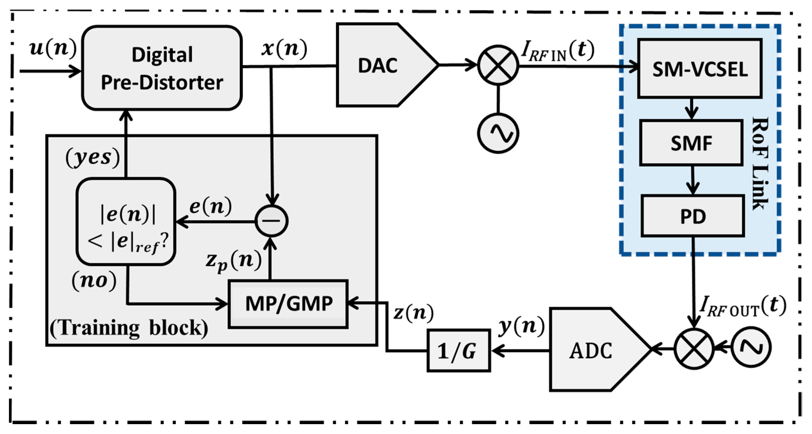
The ILA is utilized for the DPD model coefficient computation, which is characterized in Figure 5. In the training phase, the coefficients for the predistortion are computed. As explained in [6], the input of predistorter comes through the RoF output where . G represents the gain of the RoF link. The estimation of coefficients is performed using the least squares algorithm. As soon as the error converges, the coefficients are fed to the DPD block. The MP and GMP model utilized is discussed below.
3.1.1. Memory Polynomial Model
The Memory Polynomial (MP) model is an inverse nonlinear model that has been previously used for direct and inverse modeling of power amplifier (PA) nonlinearities. The MP model is a conciliation between memoryless and full Volterra nonlinearity as it carries a diagonal memory. The output of the predistorter raining block is in this case:
where is the model coefficients, represents nonlinearity order, shows memory depth and is the predistorter input sequence.
3.1.2. Generalized Memory Polynomial Model
The GMP method was implemented for VCSEL-based RoF in [15,17,18] and DFB-based links in [6,10]. The GMP model is evinced as:
In Equation (7), represent the input and output, respectively, while , and symbolize signal and envelope coefficients, signal and lagging envelope coefficients and signal leading envelope coefficients, respectively. , are the orders of nonlinearity; represent the depths of memory; shows the leading and symbolizes the lagging delay tap lengths, respectively.
3.2. Estimation Algorithm
The estimation starts with collecting the coefficients, e.g., , and into a R × 1 vector . represents the total number of coefficients. is associated with a signal whose time is sampled over the same period. Coefficients are associated with signal . represents the collection of all such vectors into a × matrix. Upon convergence, the output of the predistorter training block becomes and hence, . For a total number of samples equal to , the output can be written as follows:
where and , while is a R × 1 vector that contains the set of coefficients , and The LS solution is the solution for the following equation expressed as:
The LS solution that minimizes the cost function is expressed as
4. Complexity Considerations
The advanced variations in Volterra series can be obtained by changing memory depth and nonlinearity order to higher numbers. However, the computational complexity has to be considered as shown in Eq. 11. This means that while selecting the DPD model and its complexity, a smart tradeoff between complexity and performance can be made accordingly. For a comparative evaluation of NN and GMP methods in terms of complexity and performance, we evaluate expressions for each method in terms of its complexity. The total coefficients in the GMP method can be found by:
Similarly, the numerals in the NN model are expressed as:
This means that in the case of NN, the complexity rises accordingly with the number of hidden layers and neurons per hidden layer. For instance, if we consider one layer, the complexity grows linearly by increasing neurons. However, if more than one layer is considered, with increasing the number of neurons, the complexity will scale quadratically. Similarly, if we consider GMP, there are eight parameters which can add to the complexity; however, for simplicity, if they are considered to be the same, the number of coefficients is 6 when all variables are kept equal to 1, and it increases to 546 if the variables are given the same value equal to 6.
The parameters utilized in the NN are summarized below in Table 1.
5. Experimental Setup
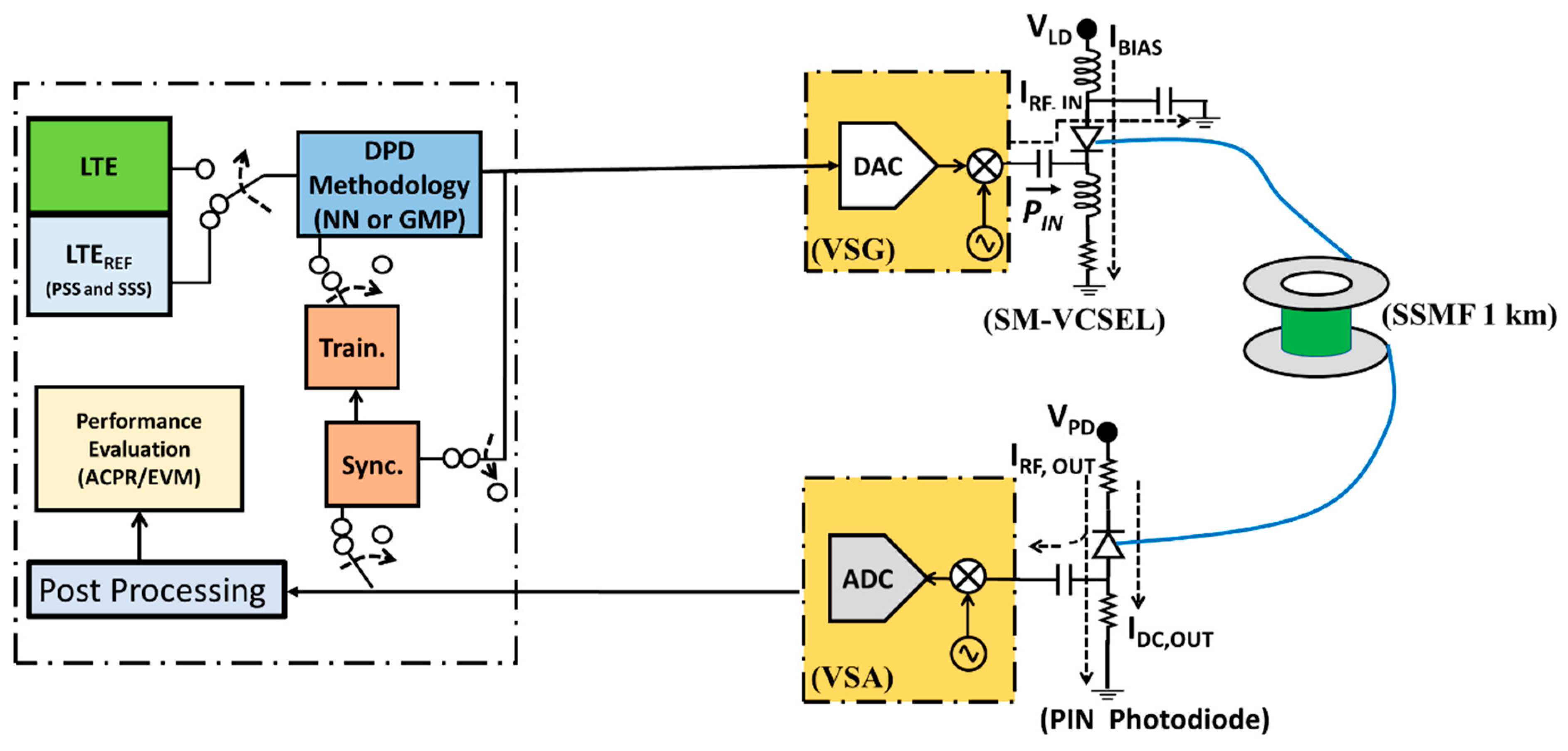
The experimental setup is presented in Figure 6, similar to the one that we presented in [17]; however, the DPD-NN-based method is an upgradation of this bench. An RoF link comprising an SM-VCSEL laser with an 850 nm wavelength is connected to a Standard Single Mode Fiber (SSMF) of 1 km. The optical signal is detected by a photodiode with a 3.4 GHz of bandwidth. The biasing current is set as so that the power consumption is at an acceptable level, while the threshold current, so that it is not very close to the threshold level. We use an inhouse software realized on MATLAB that emulates 20 MHz LTE with 256 QAM modulation baseband signal oversampled at 122.8 MSa/s. In the first phase, this signal is upconverted by a Vector Signal Generator (VSG) at a carrier frequency of 2.4 GHz. This is passed through an RoF link, and performance evaluation is carried out at the receiver with the Rohde and Schwarz FSW signal and spectrum analyzer used as a vector signal analyzer (VSA). In this step, the performance evaluation is recorded without the use of DPD block, i.e., No DPD.
In the second phase, the baseband signal oversampled at 122.8 MSa/s is fed into the DPD block and is upconverted at 2.4 GHz via VSG which is then fed to the optical link. The received signal at VSA is fed to the DPD training phase. Here, initially, the primary synchronization sequence and secondary synchronization sequence available in the LTE reference frames are engaged for synchronization between input and output (Figure 2). This block is responsible for the synchronization by finding the cross correlation by employing the M-part correlation method [34]. This operation is followed by employing the photodiode (PD) model to obtain the predistorter coefficients (Figure 2).
For the DPD validation phase, the switches move to the opposite direction, as shown in Figure 2. The evaluation is accomplished for the general LTE frames, which includes sampling, predistortion and passing them to the VSG. The nonlinear properties of the RoF link fluctuate slowly due to thermal effects and ageing of the components, which makes us assume that real-time processing in the adaptation is not required. Table 2 summarizes the parameters utilized in this work.
6. Experimental Results and Discussion
In this section, experimental results are presented and discussed. All the parameters utilized in these experiments are fixed. As mentioned before, 1 km SSMF is utilized, while memory depths and nonlinearity orders , , are also fixed. In addition to this, biasing and threshold currents for biasing SM-VCSEL laser are also fixed.
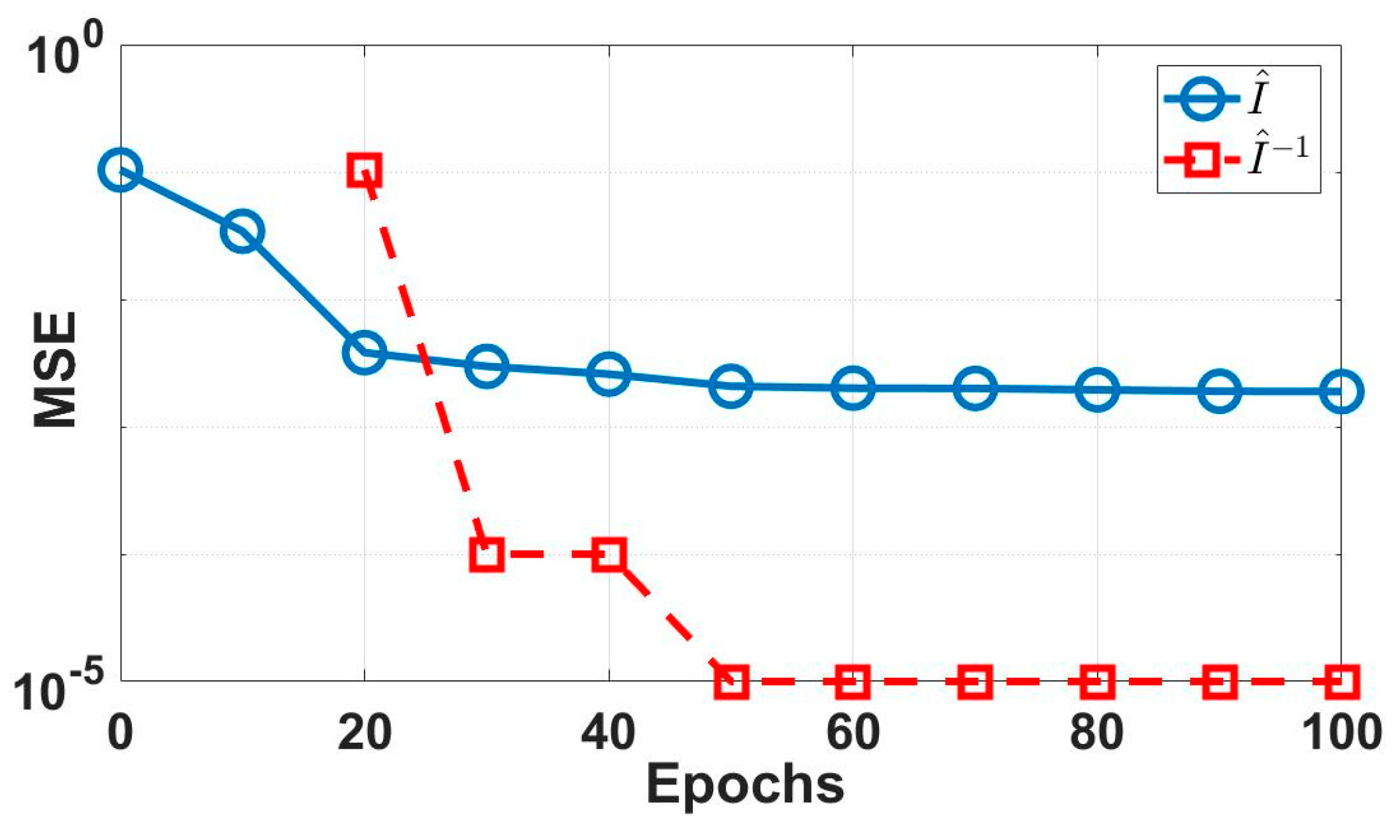
Figure 7 presents a comparison of experimental mean squared error (MSE) loss training for the NNs. It can be observed that the minimum MSE reached by the RoF NN model is 0.00189. This residue can be attributed to memory management and noise impairments in the data. Similarly, the DPD NN learns the predistortion profile for the RoF NN model. Once the learning converges, the DPD NN achieves an MSE approximately near to zero that equals . It should be noted that this is a training loss for DPD with respect to the RoF NN model. On the basis of our previous findings in [6,12], we chose memory depths and nonlinearity orders , , .
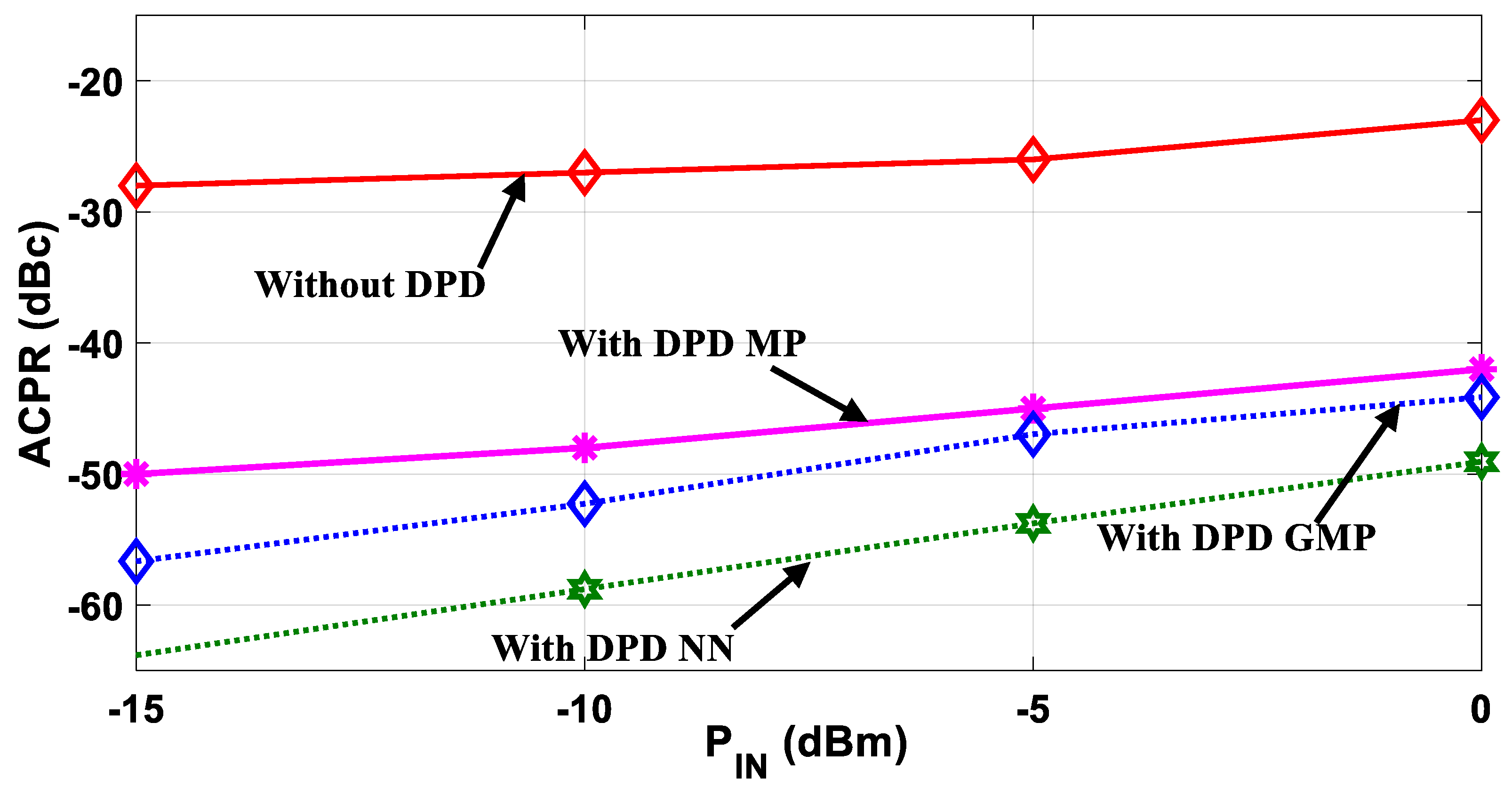
In Figure 8, the experimental findings are reported for ACPR for varying input powers. Since radio frequency (RF) input power can change with a change in application or scenario, it is of fundamental importance to check the effectiveness of the techniques used. The trend in Figure 8 confirms that the NN-based DPD method is performs better compared to GMP-based DPD. It can be noted that at a relatively higher RF input power of 5 dBm, the output ACPR is −25 dBc without DPD, −35 dBc with DPD-GMP and −40 dBc with the DPD-NN method, respectively.
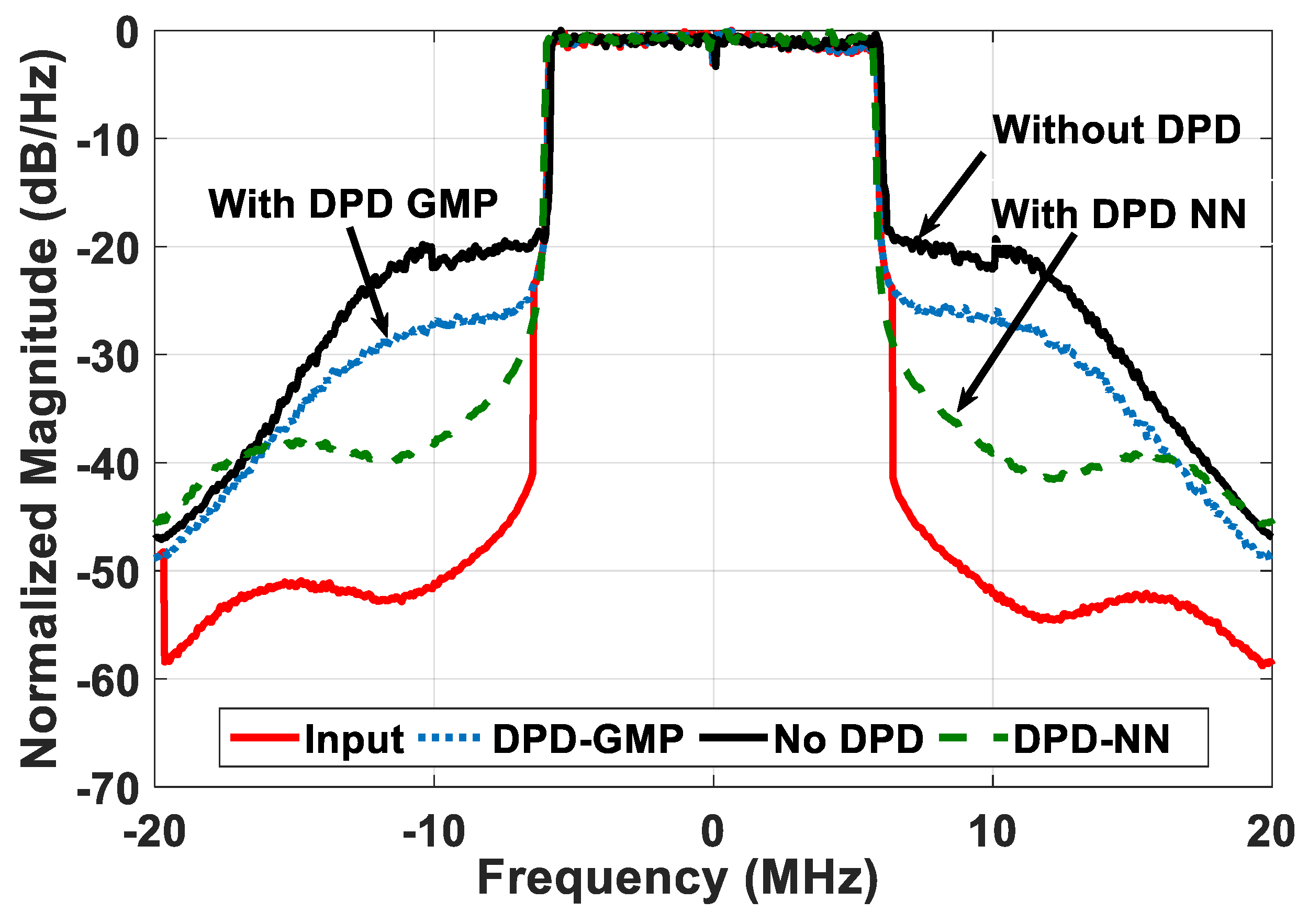
Similarly, Figure 9 represents the Power Spectral Density (PSD), i.e., spectral regrowth of the received output signal with and without DPD for 0 . In the case of DPD, the two methodologies are shown. The DPD with GMP method is represented by the blue dashed line, while DPD-NN is shown using the green dash-dotted line. The output signal without DPD is shown by the red solid line. It can be observed that DPD-NN results in lower spectral regrowth with respect to GMP. Indeed, NN results in lower spectral regrowth as compared to GMP.
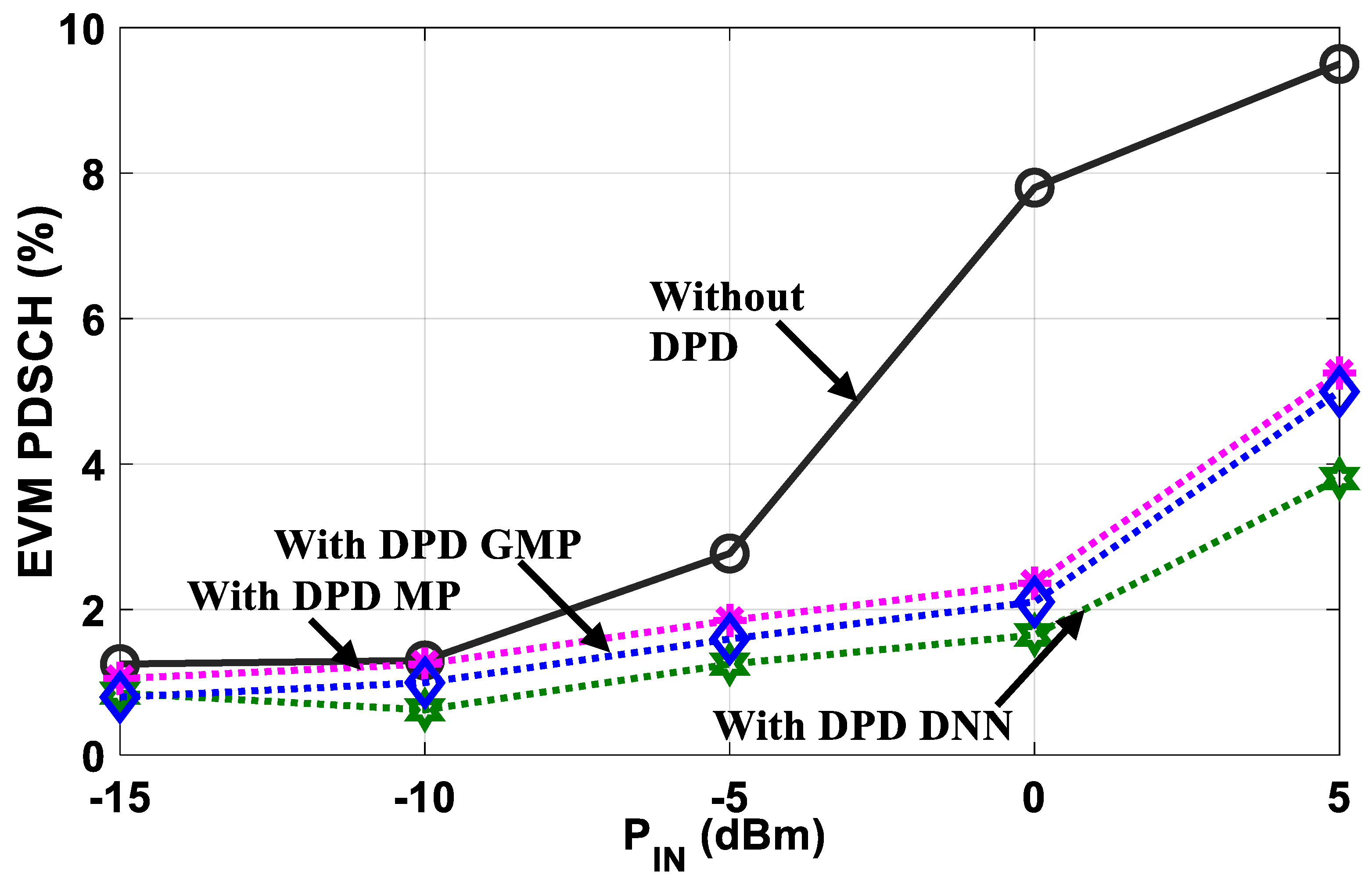
In addition to ACPR evaluation, EVM performance is evaluated, depicted in Figure 10, by sweeping the RF input power. It is evident that EVM results also show that DPD NN results in better reduction as compared to GMP. The dynamic range of the NN method is 5 dBs higher than the GMP method. This further confirms that the NN method outperforms Volterra-based methods. The overall results are summarized in Table 3.
7. Real Time Realization of the NN DPD Method
Bringing the feedback signal from the BS to RAU is among the main challenging task in the adaptive recompense of the RoF link. This is due to possible nonlinearity of the feedback link; in fact, it can be as nonlinear as the RoF link, which is compensated for. The present work is based on the fact that the predistorter identifies only the nonidealities that it needs to compensate. Since it is assumed that the nonlinear feedback connection is uncompensated, it would destroy the performance of the compensation. In other words, this means that an approach is utilized where the RoF link is first compensated for using a postdistorter, and the known training signal from the RAU is used here. After that, the already compensated for downlink RoF link can be used as a feedback connection for the compensation [3].
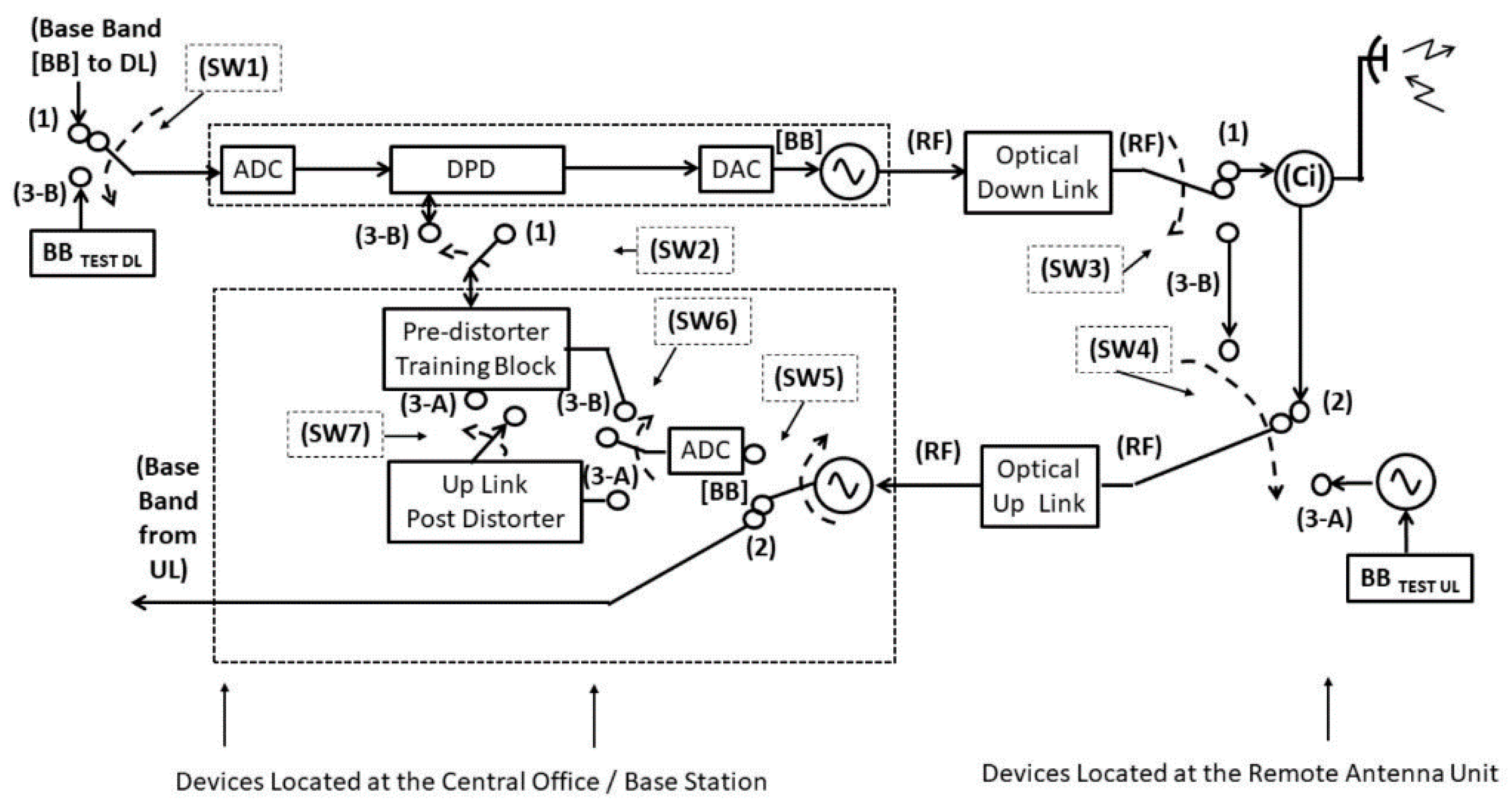
However, as a possible feedback scenario, Figure 11 represents a realistic implementation of an adaptive DPD that shifts complex processing of the signals at the Central Office / Base Transmit Station (CO-BTS). In the figure, switches SW1, SW2 and SW3 are in configuration (1), and switches SW4 and SW5 are in configuration (2), while SW6, SW7 are not influent.
This correlates to the “normal” operation of the bidirectional link. Indeed, the (DPD) is trained and performs a requisite processing of the digitized baseband signal, which is eventually brought back to analog form and modulated at radiofrequency (RF). After having passed through the Optical DL, the signal enters a circulator (Ci) that allows the transmission of the signal through a remote antenna unit (RAU).
Conversely, the signal received by the RAU passes through (Ci) and is transmitted to the Optical UL up to the CO/BS. Then, the signal is brought back to BB and processed by the CO-BTS (operation not shown). When switches SW4, SW6 and SW7 are set to configuration (3-A), and SW5 is connected to the ADC, a postdistortion operation is accomplished with reference to the UL. An RF test signal is sent through the Optical UL and arrives at the CO-BTS.
The characteristic parameters of the DPD methods (generalized/Memory Polynomials/DNN) are fed to the PD Controller. The predistorter controller block is able to augment the sampled version of the baseband signal that was received at the RAU similarly to if the operation of demodulation and sampling were performed at the RAU. It is anticipated that the nonlinear properties of the UL are stable across time, and so this process is seldom performed at the same frequency at which the DPD training is acquired.
The training of the digital predistorter is accomplished when switches SW1, SW2, SW3, SW4 and SW6 are set to configuration (3-B), while SW5 is connected to the ADC (SW7 not influent). This is the configuration described in the submitted work, where the digital predistortion block compares the transmitted and received sampled versions of the transmitted BB signal. It can be additionally discerned that a slight modification in the architecture shown in Figure 11 will utilize the Up-Link postdistortion mechanism for a reliable DPD feedback system.
8. Hardware Limitations
Machine learning solutions eminently depend on hardware resources for the computational handling of the task. From this experiment, we observe that training the model for 1 km of link length and utilized RF input power is not a tedious task. The training efficiency is converged in good proportions with one hidden layer and 30 neurons per layer. However, with optimized training, selection of the number of hidden layers and size of neurons per layer, linearization of longer link distances and higher bandwidths can be implied. Higher bandwidth signals such as multiple LTE carriers or 5G new radio (NR) waveforms would lead to elevated complexity of DPD performance due to vigorous PAPR. Eventually, this will lead to an overall bandwidth elevation in the baseband memory of the model.
9. Possible Future Directions
As far as future directions are concerned, the commercial viability of the current ML-based RoF networks is questionable. As pointed out in [30], hyperparameter selection is a critical point, as these parameters are tuned manually for now. There are no clear-cut rules or directions for the selection of these hyperparameters. Therefore, deep theoretical understanding of these ML algorithms is needed so they can be applied in practical RoF network management and resource allocation applications.
Similarly, availability of large data sets is a stringent prerequisite in terms of overhead, time and energy costs for using ML schemes effectively. This can be challenging for network failure-related training sets, as realistic networks have efficient designs that normally have the minimum possibility of network faults. As explained in [35,36], a possible solution is the transfer learning principle that eradicates the overheads linked with these trainings if the network changes relatively slowly over time.
Moreover, it is expected and also shown in this work that ML-based solutions will improve performance as compared to conventional methods, but this efficiency increase will involve additional costs, and this needs to be handled carefully.
10. Conclusions
This paper presents a novel unprecedented DPD-based NN architecture and training method for RoF link efficiency enhancement. A comparative evaluation study was carried out experimentally between NN- and Volterra (MP/GMP)-based DPD methods, and system potential was measured in terms of MSE, ACPR and EVM. The results validate that NN-based DPD reduces spectral regrowth by 22 dBs at 0 dBm of input power, and EVM is reduced from 8.1% to 1.5%, while the GMP-based method reduces ACPR by 14 dB and EVM to 2.3%. This asserts that an NN-based DPD method enhances the RoF link performance as compared to a GMP-based method already at a very low complexity. The extension of NN to include memory effects and tuning of hyper parameters for higher linearization link lengths and utilization of 5G NR multiband signals is envisaged in future work.
Author Contributions
Conceptualization, M.U.H. and K.K.; Data curation, H.J.; Formal analysis, K.K.; Funding acquisition, M.U.H. and M.R.; Investigation, M.U.H.; Methodology, M.U.H.; Software, M.A.; Supervision, M.U.H., M.R. and H.J.; Writing—original draft, M.U.H.; Writing—review and editing, H.J. All authors have read and agreed to the published version of the manuscript.
Funding
This research received no external funding.
Data Availability Statement
The data presented in this study are available on request from the corresponding author.
Acknowledgments
Authors would like to thank Amir Khawaja for their fruitful comments and suggestions.
Conflicts of Interest
The authors declare no conflict of interest.
References
- Hadi, M.U.; Awais, M.; Raza, M. Multiband 5G NR-over-Fiber System Using Analog Front Haul. In Proceedings of the 2020 International Topical Meeting on Microwave Photonics (MWP), Matsue, Japan, 23–26 November 2020; pp. 136–139. [Google Scholar]
- 3GPP, User Equipment (UE) Radio Transmission and Reception; Part 3: Range 1 and Range 2 Interworking Operation with Other Radios, 2019, TS 38.101-3 Version 16.0.0 Release 16. Available online: https://0-ieeexplore-ieee-org.brum.beds.ac.uk/document/9314547 (accessed on 5 January 2021).
- Hadi, M.U. Digital Signal Processing Techniques Applied to Radio over Fiber Systems. Ph.D. Thesis, Engineering Alma Mater Studiorum University of Bologna, Bologna, Italy, 2020. [Google Scholar] [CrossRef]
- Khurshid, K.; Khan, A.A.; Siddiqui, H.; Rashid, I.; Hadi, M.U. Big Data Assisted CRAN Enabled 5G SON Architecture. J. ICT Res. Appl. 2019, 13, 93–106. [Google Scholar] [CrossRef]
- Hadi, M.U.; Nanni, J.; Polleux, J.L.; Traverso, P.A.; Tartarini, G. Direct digital predistortion technique for the compensation of laser chirp and fiber dispersion in long haul radio over fiber links. Opt. Quantum Electron. 2019, 51, 205. [Google Scholar] [CrossRef]
- Hadi, M.U.; Kantana, C.; Traverso, P.A.; Tartarini, G.; Venard, O.; Baudoin, G.; Polleux, J.L. Assessment of digital predistortion methods for DFB-SSMF radio-over-fiber links linearization. Microw. Opt. Technol. Lett. 2020, 62, 540–546. [Google Scholar] [CrossRef]
- Zhang, X.; Zhu, R.; Shen, D.; Liu, T. Linearization Technologies for Broadband Radio-Over-Fiber Transmission Systems. Photonics 2014, 1, 455–472. [Google Scholar] [CrossRef]
- Li, H.; Verplaetse, M.; Verbist, J.; van Kerrebrouck, J.; Breyne, L.; Wu, C.H.; Bogaert, L.; Moeneclaey, B.; Yin, X.; Bauwelinck, J.; et al. Real-Time 100-GS/s Sigma-Delta Modulator for All-Digital Radio-Over-Fiber Transmission. J. Lightwave Technol. 2020, 38, 386–393. [Google Scholar] [CrossRef] [Green Version]
- Hadi, M.U.; Jung, H.; Ghaffar, S.; Traverso, P.A.; Tartarini, G. Optimized digital radio over fiber system for medium range communication. Opt. Commun. 2019, 443, 177–185. [Google Scholar] [CrossRef]
- Wang, J.; Jia, Z.; Campos, L.A.; Knittle, C. Delta-Sigma Modulation for Next Generation Fronthaul Interface. J. Lightwave Technol. 2019, 37, 2838–2850. [Google Scholar] [CrossRef]
- Hadi, M.U.; Traverso, P.A.; Tartarini, G.; Jung, H. Experimental characterization of Sigma Delta Radio over fiber system for 5G C-RAN downlink. ICT Express 2020, 6, 23–27. [Google Scholar] [CrossRef]
- Hadi, M.U.; Jung, H.; Traverso, P.; Tartarini, G. Experimental evaluation of real-time sigma-delta radio over fiber system for fronthaul applications. Int. J. Microw. Wirel. Technol. 2020, 1–10. [Google Scholar] [CrossRef]
- Hadi, M.U.; Murtaza, G. Enhancing distributed feedback-standard single mode fiber-radio over fiber links performance by neural network digital predistortion. Microw. Opt. Technol. Lett. 2021, 1–8. [Google Scholar] [CrossRef]
- Fuochi, F.; Hadi, M.U.; Nanni, J.; Traverso, P.A.; Tartarini, G. Digital predistortion technique for the compensation of nonlinear effects in radio over fiber links. In 2016 IEEE 2nd International Forum on Research and Technologies for Society and Industry Leveraging a Better Tomorrow (RTSI); IEEE: Bologna, Italy, 2016; pp. 1–6. [Google Scholar]
- Hadi, M.U.; Traverso, P.A.; Tartarini, G.; Venard, O.; Baudoin, G.; Polleux, J.L. Digital Predistortion for Linearity Improvement of VCSEL-SSMF-Based Radio-Over-Fiber Links. IEEE Microw. Wireless Comp. Lett. 2019, 29, 155–157. [Google Scholar] [CrossRef]
- Vieira, L.C.; Gomes, N.J. Experimental demonstration of digital predistortion for orthogonal frequency-division multiplexing-radio over fibre links near laser resonance. IET Optoelectron. 2015, 9, 310–316. [Google Scholar] [CrossRef] [Green Version]
- Hadi, M.U.; Nanni, J.; Traverso, P.A.; Tartarini, G.; Venard, O.; Baudoin, G.; Polleux, J.L. Linearity Improvement of VCSELs based Radio over Fiber Systems utilizing Digital Predistortion. Adv. Sci. Technol. Eng. Syst. J. 2019, 4, 156–163. [Google Scholar] [CrossRef] [Green Version]
- Hadi, M.U.; Nanni, J.; Venard, O.; Baudoin, G.; Polleux, J.L.; Tartarini, G. Practically Feasible Closed-Loop Digital Predistortion for VCSEL-MMF-Based Radio-over-Fiber links. Radioengineering 2020, 29, 37–43. [Google Scholar] [CrossRef]
- Liu, S.; Xu, M.; Wang, J.; Lu, F.; Zhang, W.; Tian, H.; Chang, G. A Multilevel Artificial Neural Network Nonlinear Equalizer for Millimeter-Wave Mobile Fronthaul Systems. J. Lightwave Technol. 2017, 35, 4406–4417. [Google Scholar] [CrossRef]
- Liu, S.; Mididoddi, C.K.; Zhou, H.; Li, B.; Xu, W.; Wang, C. Single-Shot Sub-Nyquist RF Signal Reconstruction Based on Deep Learning Network. In Proceedings of the 2018 International Topical Meeting on Microwave Photonics (MWP), Toulouse, France, 22–25 October 2018; pp. 1–4. [Google Scholar] [CrossRef] [Green Version]
- Yang, H.; Zeng, J.; Zheng, Y.; Jung, H.D.; Huiszoon, B.; Zantvoort, J.H.C.; Tangdiongga, E.; Koonen, A.M.J. Evaluation of effects of MZM nonlinearity on QAM and OFDM signals in RoF transmitter. In Proceedings of the 2008 International Topical Meeting on Microwave Photonics jointly held with the 2008 Asia-Pacific Microwave Photonics Conference, Gold Coast, Australia, 9 September–3 October 2008; pp. 90–93. [Google Scholar]
- Marcuse, D.; Chraplyvy, A.R.; Tkach, R.W. Effect of fiber nonlinearity on long-distance transmission. J. Lightwave Technol. 1991, 9, 121–128. [Google Scholar] [CrossRef]
- Inoue, K.; Toba, H. Wavelength conversion experiment using fiber four-wave mixing. IEEE Photonics Technol. Lett. 1992, 4, 69–72. [Google Scholar] [CrossRef]
- Vagionas, C.; Ruggeri, E.; Tsakyridis, A.; Kalfas, G.; Leiba, Y.; Miliou, A.; Pleros, N. Linearity Measurements on a 5G mmWave Fiber Wireless IFoF Fronthaul Link with analog RF beamforming and 120° degrees steering. IEEE Commun. Lett. 2020, 24, 2839–2843. [Google Scholar] [CrossRef]
- Morgan, D.R.; Ma, Z.; Ding, L. Reducing measurement noise effects in digital predistortion of RF power amplifiers. In Proceedings of the IEEE International Conference on Communications, Anchorage, AK, USA, 11–15 May 2003; Volume 4, pp. 2436–2439. [Google Scholar]
- Psaltis, D.; Sideris, A.; Yamamura, A.A. A multilayered neural network controller. IEEE Control Syst. Mag. 1988, 8, 17–21. [Google Scholar] [CrossRef]
- Eun, C.; Powers, E.J. A new volterra predistorter based on the indirect learning architecture. IEEE Trans. Signal Process. 1997, 45, 223–227. [Google Scholar]
- Paaso, H.; Mammela, A. Comparison of Direct Learning and Indirect Learning Predistortion Architectures. In Proceedings of the 2008 IEEE International Symposium on Wireless Communication Systems, Reykjavik, Iceland, 21–24 October 2008; pp. 309–313. [Google Scholar]
- Musumeci, F.; Rottondi, C.; Nag, A.; Macaluso, I.; Zibar, D.; Ruffini, M.; Tornatore, M. An overview on 934 application of machine learning techniques in optical networks. IEEE Commun. Surv. Tutor. 2019, 21, 1383–1408. [Google Scholar] [CrossRef] [Green Version]
- He, J.; Lee, J.; Kandeepan, S.; Wang, K. Machine Learning Techniques in Radio-over-Fiber Systems and Networks. Photonics 2020, 7, 105. [Google Scholar] [CrossRef]
- Hadi, M.U. Mitigation of nonlinearities in analog radio over fiber links using machine learning approach. ICT Express 2020, in press. [Google Scholar] [CrossRef]
- Hadi, M.U.; Basit, A.; Khurshid, K. Nonlinearities Mitigation in Radio over Fiber Links for Beyond 5G C-RAN Applications using Support Vector Machine Approach. In Proceedings of the 2020 IEEE 23rd International Multitopic Conference (INMIC), Bahawalpur, Pakistan, 5–7 November 2020; pp. 1–4. [Google Scholar]
- Anttila, L.; Handel, P.; Valkama, M. Joint mitigation of power amplifier and I/Q modulator impairments in broadband direct-conversion transmitters. IEEE Trans. Microw. Theory Tech. 2010, 58, 730–739. [Google Scholar] [CrossRef]
- Yu, Y.; Zhu, Q. A novel time synchronization for 3GPP LTE cell search. In Proceedings of the 2013 8th International Conference on Communications and Networking in China (CHINACOM), Guilin, China, 14–16 August 2013; pp. 328–331. [Google Scholar] [CrossRef]
- Zhang, J.; Xia, L.; Zhu, M.; Hu, S.; Xu, B.; Qiu, K. Fast remodelling for nonlinear distortion mitigation based on transfer learning. Opt. Lett. 2019, 44, 4243–4246. [Google Scholar] [CrossRef]
- Pan, S.J.; Yang, Q. A survey on transfer learning. IEEE Trans. Knowl. Data Eng. 2010, 22, 1345–1359. [Google Scholar] [CrossRef]
Figure 1.
Block diagram of Centralized/Cloud Radio Access Network (C-RAN)-based 5G application system comprising backhaul, fronthaul and application scenarios such as stadiums, railways, transport and factories.
Figure 1.
Block diagram of Centralized/Cloud Radio Access Network (C-RAN)-based 5G application system comprising backhaul, fronthaul and application scenarios such as stadiums, railways, transport and factories.

Figure 2.
Block schematic of analog radio over fiber (A-RoF), digital radio over fiber (D-RoF) and ΣΔ-RoF downlinks. Freq. Upconv.: Frequency Upconverter, BB: baseband, Tx: Transmitter, ΣΔMOD: Sigma-Delta Modulator, Data Rec.: Data Recovery block.
Figure 2.
Block schematic of analog radio over fiber (A-RoF), digital radio over fiber (D-RoF) and ΣΔ-RoF downlinks. Freq. Upconv.: Frequency Upconverter, BB: baseband, Tx: Transmitter, ΣΔMOD: Sigma-Delta Modulator, Data Rec.: Data Recovery block.

Figure 3.
Schematic showing RoF system utilizing a neural network (NN) digital predistortion (DPD) system and RoF NN model. After transmitting through the RoF link, the input and output of RoF are used to model RoF NN model . Once trained, by backpropagating the error through , training of is performed. This DPD RoF model is then used with the RoF link to perform linearization. Predistortion is carried out in a digital baseband so ADC and DACs are omitted.

Figure 4.
Schematic showing block diagram of NN structure used in this article, feedforward fully connected (FC) NN. FC-NN contained hidden layers and neurons per hidden layer.
Figure 4.
Schematic showing block diagram of NN structure used in this article, feedforward fully connected (FC) NN. FC-NN contained hidden layers and neurons per hidden layer.

Figure 5.
Schematic of indirect learning architecture for the Memory Polynomial (MP)/ Generalized Memory Polynomial (GMP)-based DPD methodology.
Figure 5.
Schematic of indirect learning architecture for the Memory Polynomial (MP)/ Generalized Memory Polynomial (GMP)-based DPD methodology.

Figure 6.
Block diagram of experimental testbed. DPD implemented for general LTE frames. DPD-NN or DPD-MP/GMP can be selected from the choice present in the simulator.
Figure 6.
Block diagram of experimental testbed. DPD implemented for general LTE frames. DPD-NN or DPD-MP/GMP can be selected from the choice present in the simulator.

Figure 7.
Experimental results for comparison of experimental MSE training loss for the NNs.

Figure 8.
Experimental results for Adjacent Channel Power Ration (ACPR) results versus radio frequency input power for output with DPD-NN, DPD-MP, DPD-GMP and without DPD.
Figure 8.
Experimental results for Adjacent Channel Power Ration (ACPR) results versus radio frequency input power for output with DPD-NN, DPD-MP, DPD-GMP and without DPD.

Figure 9.
Spectral regrowth for output with DPD-NN, DPD-GMP and without DPD.

Figure 10.
Experimental results for Error Vector Magnitude (EVM) received signal without and with linearization (DPD-NN and DPD-MP/GMP).
Figure 10.
Experimental results for Error Vector Magnitude (EVM) received signal without and with linearization (DPD-NN and DPD-MP/GMP).

Figure 11.
Possible realization of an adaptive predistortion scheme.


Table 1.
NN specifications utilized.
| Specifications | Values |
|---|---|
| Optimizer | ADAM |
| Loss Function | Mean Square Error |
| Hidden Layers | 6 |
| Neurons per layer | 25 |
| Hidden Layer Type | ReLu |
| Regularization | L1 |
Table 2.
Experimental setup parameter values.
| Link Components | Values |
|---|---|
| SM-VCSEL | |
| Wavelength | 850 nm |
| 5 mA | |
| 2 mA | |
| RIN | −130 dB/Hz |
| SSMF | |
| Length | 1 km |
| Attenuation | 3 dB/km |
| PD | |
| Responsivity | 0.71 A/W |
| Bandwidth | 2.5 GHz |
Table 3.
Comparison among DPD methods for 0 dBm input power.
| Model | ACPR (dBc) | EVM (%) |
|---|---|---|
| No DPD | −25 | 8 |
| MP | −35 | 2.2 |
| GMP | −40 | 2 |
| NN | −50 | 1.4 |
Publisher’s Note: MDPI stays neutral with regard to jurisdictional claims in published maps and institutional affiliations. |
© 2021 by the authors. Licensee MDPI, Basel, Switzerland. This article is an open access article distributed under the terms and conditions of the Creative Commons Attribution (CC BY) license (http://creativecommons.org/licenses/by/4.0/).
Share and Cite
MDPI and ACS Style
Hadi, M.U.; Awais, M.; Raza, M.; Khurshid, K.; Jung, H. Neural Network DPD for Aggrandizing SM-VCSEL-SSMF-Based Radio over Fiber Link Performance. Photonics 2021, 8, 19. https://0-doi-org.brum.beds.ac.uk/10.3390/photonics8010019
AMA Style
Hadi MU, Awais M, Raza M, Khurshid K, Jung H. Neural Network DPD for Aggrandizing SM-VCSEL-SSMF-Based Radio over Fiber Link Performance. Photonics. 2021; 8(1):19. https://0-doi-org.brum.beds.ac.uk/10.3390/photonics8010019
Chicago/Turabian StyleHadi, Muhammad Usman, Muhammad Awais, Mohsin Raza, Kiran Khurshid, and Hyun Jung. 2021. "Neural Network DPD for Aggrandizing SM-VCSEL-SSMF-Based Radio over Fiber Link Performance" Photonics 8, no. 1: 19. https://0-doi-org.brum.beds.ac.uk/10.3390/photonics8010019
Note that from the first issue of 2016, this journal uses article numbers instead of page numbers. See further details here.