Independently Controlling Stochastic Field Realization Magnitude and Phase Statistics for the Construction of Novel Partially Coherent Sources


Department of Engineering Physics, Air Force Institute of Technology, 2950 Hobson Way, Dayton, OH 45433, USA
Photonics 2021, 8(2), 60; https://0-doi-org.brum.beds.ac.uk/10.3390/photonics8020060
Submission received: 24 December 2020
/
Revised: 24 January 2021
/
Accepted: 19 February 2021
/
Published: 22 February 2021
(This article belongs to the Special Issue Structured Light Coherence)
Abstract
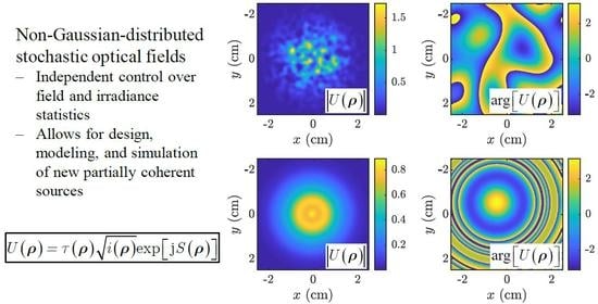
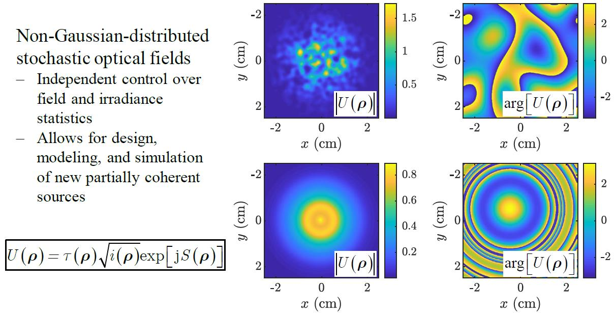
:In this paper, we present a method to independently control the field and irradiance statistics of a partially coherent beam. Prior techniques focus on generating optical field realizations whose ensemble-averaged autocorrelation matches a specified second-order field moment known as the cross-spectral density (CSD) function. Since optical field realizations are assumed to obey Gaussian statistics, these methods do not consider the irradiance moments, as they, by the Gaussian moment theorem, are completely determined by the field’s first and second moments. Our work, by including control over the irradiance statistics (in addition to the CSD function), expands existing synthesis approaches and allows for the design, modeling, and simulation of new partially coherent beams, whose underlying field realizations are not Gaussian distributed. We start with our model for a random optical field realization and then derive expressions relating the ensemble moments of our fields to those of the desired partially coherent beam. We describe in detail how to generate random optical field realizations with the proper statistics. We lastly generate two example partially coherent beams using our method and compare the simulated field and irradiance moments theory to validate our technique.
1. Introduction
The design and physical realization of spatially partially coherent light is a highly active area of beam-control research. One of the foundational papers on the subject is “Designing genuine spatial correlations functions” by F. Gori and M. Santarsiero [1]. Cited hundreds of times since publication, the paper presents a simple recipe for creating any physically realizable partially coherent source. This recipe is expressed in the form of a superposition integral, namely,
where W is the source’s cross-spectral density (CSD) function [2,3], p is a positive, real function, H is the kernel, and . In Equation (1), the dependence of W, p, and H on radian frequency is assumed and suppressed. Since p and H, for the most part, can be arbitrarily chosen, Equation (1) has been used to create all manner of random optical beams. More information on these sources can be found in the subject reviews and books in References [4,5,6,7,8,9].
The superposition rule, as Equation (1) is now known, specifies the CSD function, or second-order field moment, of a partially coherent source. It does not, however, stipulate the fourth-order field moment, more specifically, the second-order moment of irradiance or covariance of irradiance. With the exception of propagation through turbulent media, where the primary goal has been to quantify how partial coherence reduces the variance of irradiance (captured in a moment called the scintillation index) [4,10,11,12], the covariance of irradiance has been a secondary concern to designers of random sources [6,7,13,14,15,16,17,18,19,20,21,22,23].
The reason for this is because the underlying electric fields giving rise to the desired partially coherent source are assumed (in most cases, with very good reason) to be Gaussian distributed. According to the Gaussian moment theorem, all statistical moments greater than second order simplify to sums and products of first- and second-order moments [3,4,24]. The result being that the covariance of irradiance is completely determined by the CSD function, and the scintillation index is always equal to one. Physically, this means that the stochastic field realizations comprising the partially coherent source are fully developed speckle fields, where, in the case of uniformly correlated or Schell-model sources, the average size of a speckle is given by the width of the normalized CSD function, also known as the spatial coherence function [24].
In this paper, we present a method to independently control the field and irradiance moments of a partially coherent source. This new technique creates stochastic field instances with non-Gaussian statistics, and therefore allows for the modeling and simulation of random beam scattering and propagation through turbulent media. In addition, this approach can be used to engineer new partially coherent sources with potentially interesting and exploitable characteristics.
In the next section, we describe our random field model, which is the product of a deterministic function corresponding to the beam shape and two statistically independent random processes—one corresponding to the field’s phase and the other to its irradiance. We then derive relationships between the phase and irradiance moments and the desired source’s CSD function and covariance of irradiance. We end this section by presenting how to generate phase and irradiance instances, with the proper statistics, to produce a random field realization statistically consistent with the desired partially coherent source.
In Section 3, we present two examples where we apply our method to produce partially coherent sources. For the first source, we generate a Gaussian Schell-model (GSM) beam [2,4]. To validate our approach, we compare the resulting field and irradiance sample moments to theory and those of another GSM beam generated using circular complex Gaussian (CCG) random numbers [17,18,20]. In the second example, we create a new partially coherent beam, where the CSD function has the form of a Lajunen and Saastamoinen nonuniformly correlated (NUC) source [25], the irradiance is log-normally distributed, and the covariance of irradiance takes a pseudo-Schell model form [26]. We again compare the sample field and irradiance moments to theory to verify that we have indeed produced the desired source. Lastly, we conclude with a summary of our work.
2. Materials and Methods
2.1. Stochastic Field Model
We begin this section with our model for a random optical field realization:
where is complex, deterministic, and physically represents the beam shape, i is a real, positive random function corresponding to the irradiance, and S is a real random function representing the phase.
Here, we assume that the random processes i and S are statistically independent. This assumption, made ultimately out of mathematical necessity, is generally not accurate. Take, for instance, the case of fully developed speckle fields. In Reference [24], Goodman shows that while the field amplitude and phase are statistically independent at any one spatial point, they are not jointly independent at two points. This means that in computing , we could separate the expectation involving i and S into the product of two expectations; however, the same operation would be improper when computing . In this paper, we are ultimately interested in generating partially developed speckle fields (non-Gaussian-distributed fields), and unfortunately, the joint magnitude and phase statistics of such fields are generally not known. While i and S most certainly are not independent, lacking additional information, it becomes nearly impossible to proceed without assuming so. Not accounting for the correlation between i and S surely misses physical phenomena.
The important statistical moments of Equation (2) are the mean field, the CSD function, the mean irradiance, and the covariance of irradiance. These moments, in order, are
To simplify these expressions further, we let the single-position moments and be constant. Initially, this might seem like a very restrictive stipulation. However, the function in the field model accounts for the effects of spatially varying and . Equations (3)–(6) then become
where is the mean of i.
2.2. CSD Function
We now focus on the CSD function given in Equation (8). The ensemble average involving S is equivalent to the joint characteristic function (JCF) of the random variables and . In general, S could be drawn from any probability distribution. If S is a delta-correlated random process, then computing the JCF is trivial. It is also unnecessary, as a delta-correlated S, physically manifests as a spatially incoherent field, and thus, , where is the Dirac delta function. Clearly, this case is of little interest.
For an arbitrarily correlated random process, the only closed-form JCF known to the author is the Gaussian JCF [3,24]. If other-than-Gaussian JCFs exist, they can be used in Equation (8). The analysis would proceed in the same manner as that presented here, with the specifics dependent on the form of the JCF. We therefore assume that S is Gaussian distributed, substitute the Gaussian JCF into Equation (8), and simplify, ultimately producing
where is the standard deviation and is the normalized correlation function of the phase S, respectively.
We now focus on the exponential in Equation (11), hereafter referred to as M. It is clear that M plays a role in determining the coherence of the optical field—in fact, it plays the dominant role. Its form is quite restrictive in that no matter what we choose (subject to the constraints on autocorrelation functions), M will always be in the form of an exponential function. Therefore, to proceed, we should choose a form for that allows us to easily relate phase parameters, such as phase correlation length and , to those of the optical field we wish to generate. Generalizing the Gaussian forms, which are replete in the literature [3,13,14,16,27,28,29,30,31,32], we let be
where and is any real, positive function such that , , and . The restrictions on ensure that is a genuine autocorrelation function. While not yet evident, the limitation on ensures that the function p in Equation (1) is positive.
Substituting Equation (12) into Equation (11) does little to simplify M. However, we can make further progress by assuming that the field has strong phase fluctuations, such that [3,13,14,16,27,28,29,30,31,32]. This large means that M has significant value only when , or equivalently, when . Approximating Equation (12) as , substituting this into Equation (11), and simplifying yields
It is important to note that by assuming a field with strong phase fluctuations (large ), M [the exponential in Equation (13)] is a “fast function” compared to and ultimately determines the coherence of the field. It is therefore safe to further approximate Equation (13) as
We now have achieved the desired correspondence between the autocorrelation function of the phase [Equation (12)] and that of the field.
Further examination of Equation (14) reveals that the CSD function, that is, the statistics of the optical field, completely depend (with the exception of a constant) on the statistics of the phase S. This, plus the fact that Equations (9) and (10) show that the irradiance statistics depend solely on the moments of i, means that we have independent control over the field U and irradiance I statistics by controlling S and i, respectively. Although we can independently control U and I statistics, because S is Gaussian distributed and the Gaussian JCF has the form given in Equation (11), we are limited to field correlation functions of exponential type, like that in Equation (14).
Before proceeding to the irradiance moments, we briefly discuss the mean field, Equation (7). With S being Gaussian distributed, simplifies to
where is the mean of S. We stipulated above that . This large value of effectively makes . Since appears only in , it is a free parameter. We therefore let .
2.3. Covariance of Irradiance
We now turn to the irradiance moments in Equations (9) and (10), starting with . We first note that , where is called the scintillation index [4,12]. When dealing with speckle as opposed to irradiance fluctuations due to turbulence, is commonly used and is referred to as the speckle contrast [24]. Introducing into Equation (10) and rearranging the terms yields
where is the normalized covariance of irradiance, that is, . To simplify things further, we define the zero-mean random process and substitute it into Equation (16), viz.,
The expectation of i, that is, , appears only as a multiplicative constant in [Equation (9)], W in Equation (14), and here in Equation (17). Therefore, like , it is a free parameter and can be arbitrarily chosen subject to the constraint . We set , hereafter. This simplifies the mean irradiance in Equation (9) to
Equation (17) states that any can be produced if we generate a sequence of zero-mean random numbers with as its autocorrelation function. It is easy to produce such a sequence using Gaussian random numbers. However, the difficulty here is that cannot be Gaussian distributed, because that would make i Gaussian distributed. Since normal random numbers can have negative values, the Gaussian probability density function (PDF) cannot model irradiance fluctuations.
To overcome this difficulty, we use a method known by several different names in the literature—the inverse CDF (cumulative distribution function) transform method [33,34], translation [35,36,37,38], and NORTA (NORmal To Anything) [39,40]. The method starts with a correlated Gaussian random number sequence and maps it, via a non-linear transform, to a correlated non-Gaussian sequence called the target process [33,34,35,36,37,38,39,40]. If the number of discrete points in the underlying Gaussian sequence is large, translation (NORTA, etc.) yields a target realization with the desired PDF. The non-linear transform does distort the target correlation function, and there are many techniques (mostly iterative) to correct this [35,36,37,38]. Yura and Hanson [33,34] showed that target correlation function distortion caused by translation was minor. As their results attest, translation (without subsequent correction) yields highly accurate target realizations for many different PDFs and correlation functions. Here, we use Yura and Hanson’s approach to generate i. The details are provided in the following section.
2.4. Generating S and i
In this section, we discuss how to generate realizations of S and i with the proper statistics. We start with phase S.
Recall that S is a zero-mean, real, Gaussian random process with an autocorrelation function equal to
, and . In addition, is a real, positive function with , , and . Since meets the requirements for a genuine correlation function [1,2,4], we can use a variant of Equation (1) to generate realizations of S. This method was first described in Reference [41] to synthesize Gaussian distributed optical field realizations with arbitrary (genuine) correlation functions. Here, we utilize this approach to produce arbitrarily correlated, real-valued S and ultimately i realizations.
Following and modifying as necessary the analysis presented in Reference [41], an instance of S can be synthesized by evaluating the integral
where “Re” denotes the real part and is a sample function drawn from a delta-correlated, zero-mean, CCG random process. Taking the autocorrelation of Equation (20) yields a superposition integral in the form of Equation (1), namely,
Proof of this is shown in Appendix A. This is an important result as it proves that Equation (20) generates an S with the proper statistics.
Since Equation (20) must ultimately be evaluated numerically, we express it in discrete form:
where ⊙ is the Hadamard product, and are the grid spacings in the and directions, and and are discrete double indices corresponding to every combination of and coordinates, respectively. Equation (22) is a matrix-vector product, in which is a matrix, where , , , and are the number of grid points in the dimensions denoted in the subscripts; and are vectors; and S is an vector. The output vector S must be reshaped to an matrix in order to physically represent the two-dimensional phase of the field.
With S now complete, we turn our attention to generating realizations of i. As discussed at the end of the previous section, we use a process known as translation to synthesize i realizations from correlated sequences of Gaussian random numbers. These Gaussian sequences have the same first and second moments as , namely,
For this reason, we refer to them as for the remainder of the paper.
Like the phase S, the autocorrelation function of is genuine, and therefore, a realization can be produced by evaluating
where , like , is a sample function drawn from a delta-correlated, zero-mean, CCG random process. The discrete representation of Equation (24) is identical to Equation (22) with appropriate substitutions.
Having a realization, the next step is to form i by translating . This is accomplished using the non-linear transform
where is the Gaussian CDF and is the inverse target CDF [33,34,35,36,37,38,39,40]. In Equation (25), both and are parameterized by their respective means and standard deviations (assuming, in the latter case, they exist). Any probability distribution can be selected as the target PDF.
The final step is to form a random field instance U by substituting the S and i realizations into Equation (2). In the next section, we use the above procedure to generate two example partially coherent beams.
3. Results and Discussion
Here, we use the analysis from Section 2 to generate two partially coherent sources. The first is a GSM beam, which we generate in two different ways—one using the results from Section 2 (which we call the P&I technique hereafter) and the second using an established method that filters CCG random numbers (reviewed in Appendix B and called the complex screen technique) [17,18,20]. We then compare the simulation results to GSM theory. The details are presented in the next section.
The second partially coherent source is a novel stochastic beam, where the CSD function has the form of a Lajunen and Saastamoinen NUC source [25], the irradiance is log-normally distributed, and the covariance of irradiance takes a pseudo-Schell model form [26]. For brevity, we refer to this source as the NUC beam. We compare the simulated W, , field PDFs, and irradiance PDF to theory to prove that we have successfully generated the desired NUC beam. The details of this simulation are presented after the GSM beam results.
3.1. GSM Beam
Before presenting the results, we provide a brief background on GSM sources and discuss details of the simulation. A GSM beam has the following CSD function W:
where is the beam radius and is the correlation or coherence radius [2,4]. If the underlying optical fields are Gaussian distributed, the irradiance follows a negative exponential PDF, that is,
where [3,12,24]. The covariance of irradiance can easily be derived by applying the Gaussian moment theorem [3,4,24]:
To form GSM field realizations using Equation (2), we compare Equation (26) to Equation (14) and conclude that
Furthermore, , , where is the phase correlation radius, and . We then use these relations to find and in Equation (20), namely,
With being the Fourier kernel, Equation (20) equals the Fourier transform of the product of two Fourier transforms and simplifies to a convolution integral.
As a result of equaling the Fourier kernel, Equation (24), like Equation (20), simplifies to a convolution integral. Lastly, we use Equation (25) to transform to i, where is the inverse exponential CDF with .
For the simulations, we used grids that were points per side. The spacings in the x-y and - domains were m and , respectively. The GSM beam parameters were mm and mm. With , .
We generated S, i, and complex screen (CS) T realizations by evaluating Equations (20), (24), and (A7) using fast Fourier transforms. These were then substituted into Equation (2) and Equation (A5) to form GSM P&I and CS field instances. From 10,000 GSM fields each, we computed the field PDFs, irradiance PDFs, and planar (two-dimensional) cuts through W and . The simulation computer code (MATLAB® version R2018b .m files) is included as Supplementary Materials to this paper.
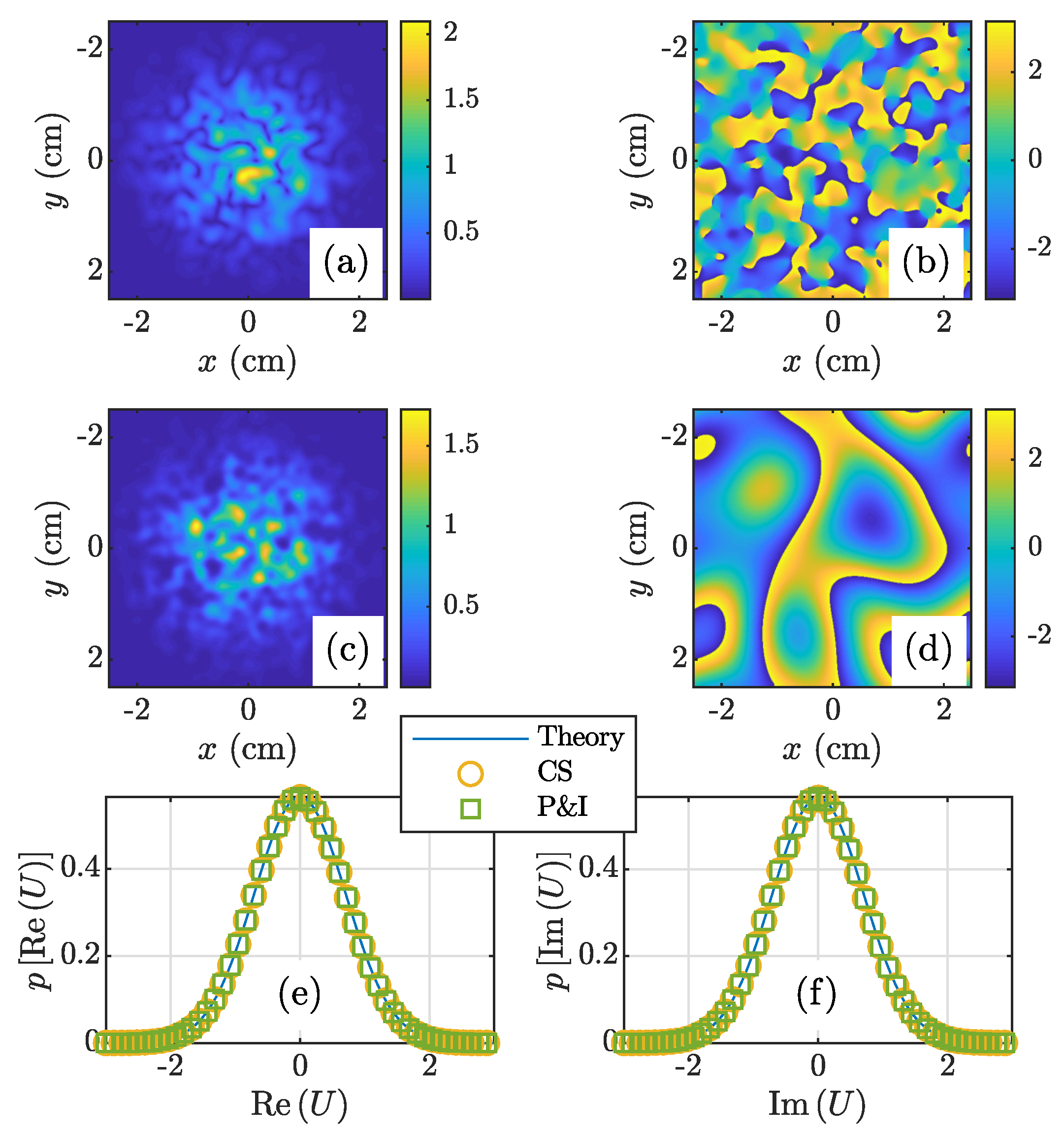
Figure 1, Figure 2 and Figure 3 show the GSM simulation results. Figure 1a–d shows a CS and P&I GSM field realization. Clearly, CS and P&I fields are different. The way that P&I fields are formed means that both S and i are continuous, independent random functions. On the other hand, CS fields are fully developed speckle fields, and while the fields themselves are continuous, the phase, in general, is not. At locations where a CS field vanishes, a phase singularity, known as a branch point, occurs [3,42]. Since the phase S in a P&I field is defined at every location, even at locations where , branch points can only ever appear in propagated P&I fields.
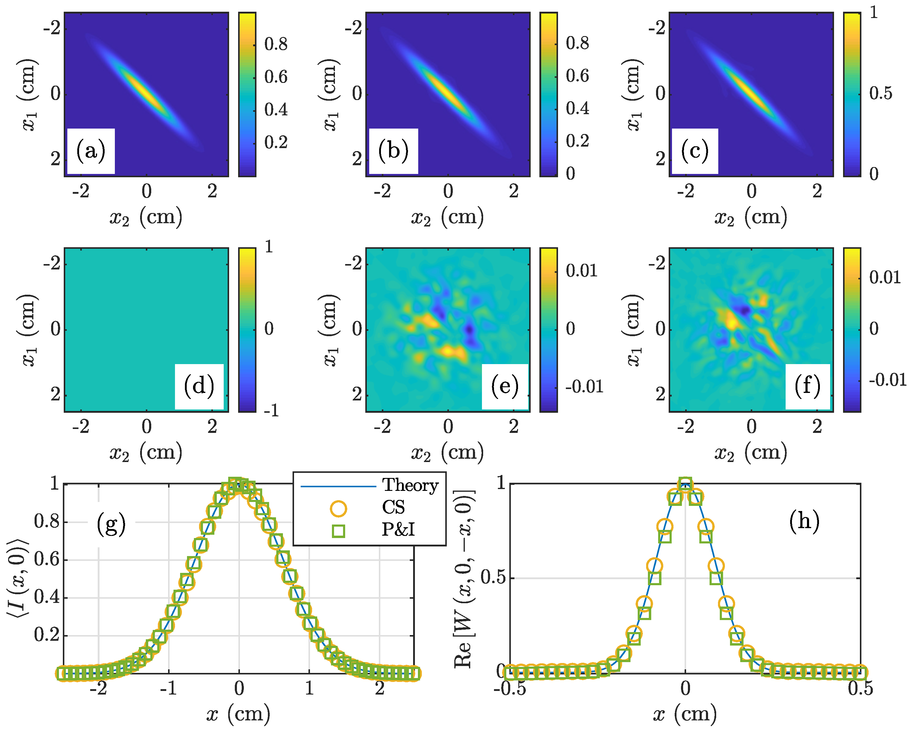
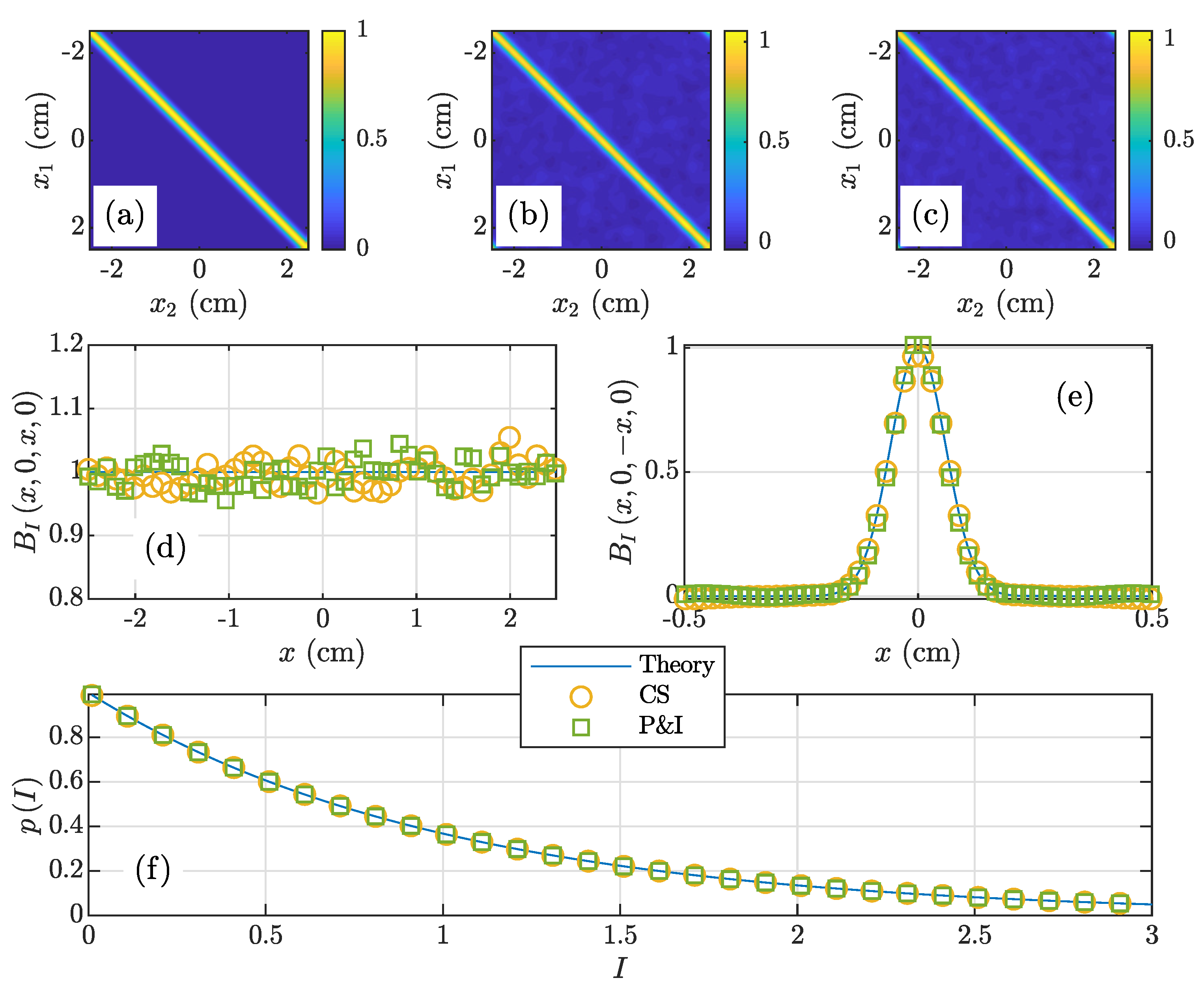
Although branch points do not appear in source-plane P&I fields, CS and P&I fields are quantitatively identical in terms of the key statistical moments discussed earlier in the paper. These results are presented in the remaining plots and figures: Figure 1e,f shows the optical field PDFs, and Figure 2 and Figure 3 show the CSD function and irradiance results, respectively. In Figure 2a–c, we report the theoretical, CS, and P&I , respectively; (d)–(f) show the corresponding ; (g) compares the slices through the mean irradiance [equal to the diagonals of (a), (b), and (c)]; and lastly, (h) compares the [equal to the anti-diagonals of (a), (b), and (c)]. Figure 3 is similarly arranged: (a)–(c) show the theoretical, CS, and P&I ; (d) compares ; (e) compares ; and (f) compares the irradiance PDFs. The agreement between theory, CS, and P&I results in these figures is excellent.
3.2. NUC Beam
We now discuss the NUC beam simulation and results. The NUC beam CSD function is
where is a real, two-dimensional vector that shifts the maximum of the correlation function away from the origin [25]. The other symbols are defined above. The PDF of irradiance is log-normal, viz.,
where the log-normal PDF parameters and are related to the i moments by
Lastly, the covariance of irradiance takes the form
where [26].
Following the same procedure used to generate a GSM field realization, we find, after comparing Equations (33) and (14), that
In contrast to the GSM beam, and Schell-model beams in general, is not the Fourier kernel, and therefore, Equation (20) must be evaluated as a matrix-vector product. This is generally a daunting task because of the size of . Here however, both and are one-dimensional in the domain. This significantly reduces the size of and simplifies Equation (20) to
For i, the autocorrelation function of is given in Equation (36). The and in Equation (24) are
where is the rectangle function defined in Reference [43]. Like and , and are one-dimensional in the domain. Equation (24) simplifies to
The last step is to transform to i using Equation (25), where is the inverse log-normal CDF with and given in Equation (35).
For the NUC beam simulations, we used spatial domain grids that were 512 points per side with a spacing equal to 97.66 m. To discretize , we used 1024 points with a spacing equal to 75.47 or for S or i, respectively. The NUC beam parameters were mm, mm, mm, , and mm. With , m.
Like the GSM simulations, we generated 10,000 P&I NUC beam field realizations and from these, computed the field PDFs, irradiance PDF, W, and . The MATLAB® scripts are included as Supplementary Materials.
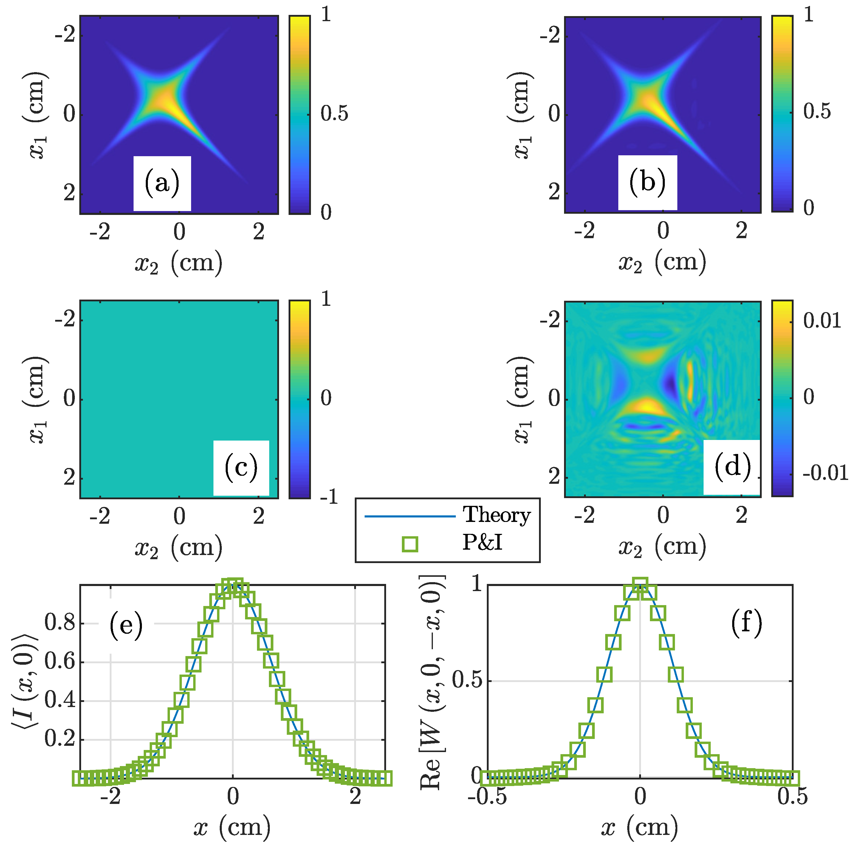
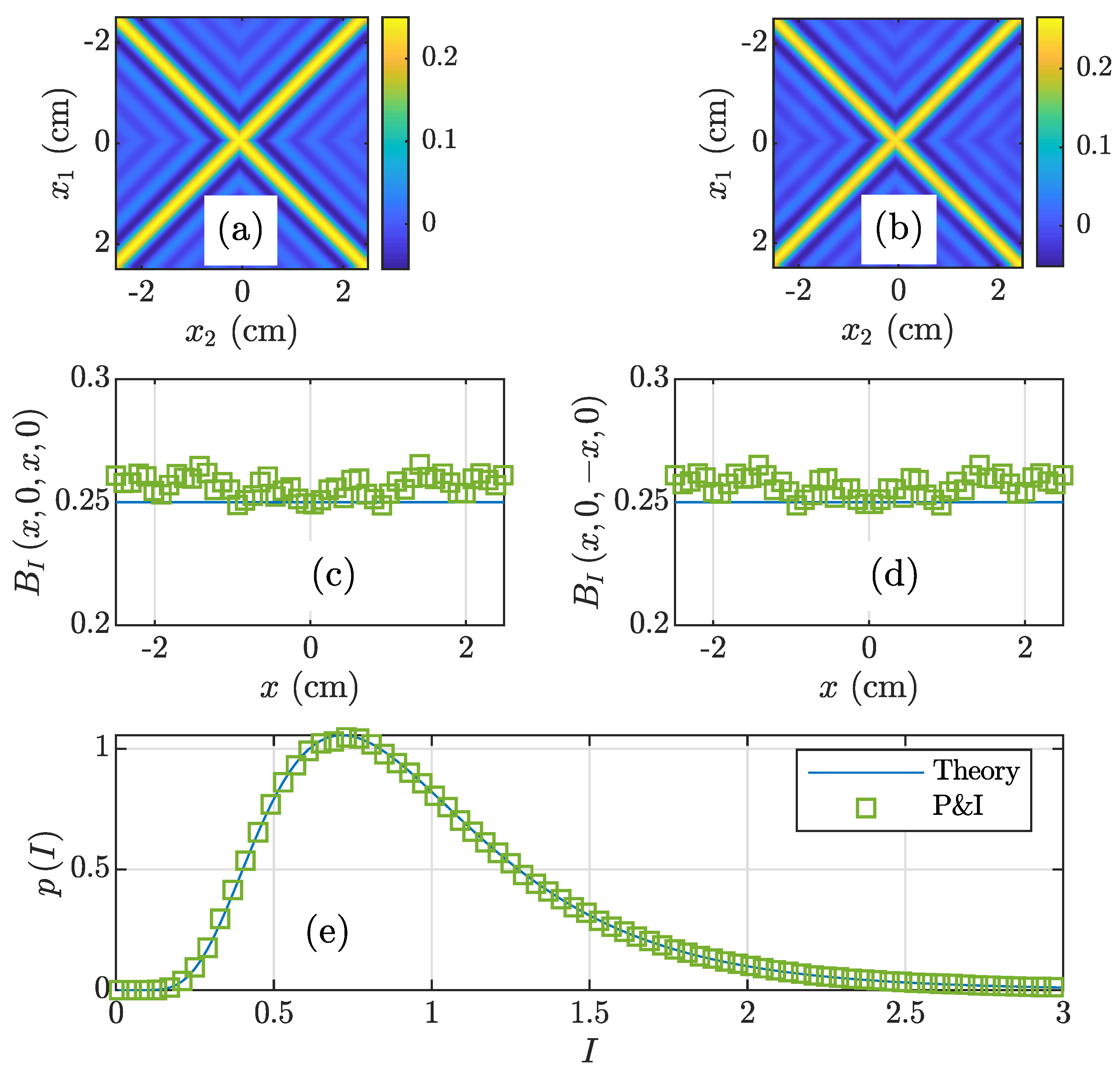
The NUC beam simulation results are shown in Figure 4, Figure 5 and Figure 6. With the exception of the CS results, the layout of the figures is identical to Figure 1, Figure 2 and Figure 3. The agreement between the theory and P&I results is again excellent. We also note that the optical field PDFs in Figure 4c,d are clearly non-Gaussian. The exact forms of these functions are unknown; we found the theoretical PDFs numerically.
4. Conclusions
In this paper, we demonstrated a new technique to synthesize partially coherent sources by independently controlling the phase and magnitude statistics of the underlying optical fields. In so doing, we generated non-Gaussian random field instances, which can be used to model interesting optical phenomena, such as random beam scattering and propagation through turbulent media, and to design new partially coherent beams with potentially interesting characteristics.
We began the analysis by presenting our model for a random field realization. Our model consisted of three functions—one deterministic function corresponding to the beam shape and two statistically independent random functions representing the phase and irradiance. We then computed ensemble moments of our field model to relate the phase and irradiance random function statistics to those of the desired partially coherent beam. We ended the analysis by describing how to generate phase and irradiance realizations that, when substituted into our model, produced a random optical field with statistics corresponding to the desired partially coherent source.
To validate our method, we generated two partially coherent sources—a GSM beam and a novel source called a NUC beam. For the GSM source, we compared simulated field and irradiance moments computed from 10,000 field realizations to the theoretical expressions. In addition, we generated GSM field instances using the complex screen approach to compare our method to an established synthesis technique. While the field realizations generated using our approach differed from complex screen fields, the agreement amongst the statistical moments was excellent. For the NUC beam, we again generated 10,000 field realizations and compared the Monte Carlo moments to the desired, theoretical expressions. The agreement was again excellent.
In conclusion, the method presented in this paper expands existing partially coherent beam synthesis approaches by permitting control over the irradiance moments of random beams. In addition, this work has the potential to be used in the design of new partially coherent sources for beam-control applications.
Supplementary Materials
The following are available online at https://0-www-mdpi-com.brum.beds.ac.uk/2304-6732/8/2/60/s1, MATLAB® version R2018b (The MathWorks, Inc., Natick, MA, USA) scripts (.m files) used to perform the simulations described in the paper.
Funding
This research received no external funding.
Institutional Review Board Statement
Not applicable.
Informed Consent Statement
Not applicable.
Data Availability Statement
The data presented in this study are available in the Supplementary Materials.
Acknowledgments
The views expressed in this paper are those of the authors and do not reflect the official policy or position of the US Air Force, the Department of Defense, or the US government.
Conflicts of Interest
The author declares no conflict of interest.
Abbreviations
The following abbreviations are used in this manuscript:
| CCG | circular complex Gaussian |
| CDF | cumulative distribution function |
| CS | complex screen |
| CSD | cross-spectral density |
| GSM | Gaussian Schell-model |
| JCF | joint characteristic function |
| NUC | nonuniformly correlated |
| NORTA | NORmal To Anything |
| probability density function |
Appendix A. Proof of Equation (21)
Starting with Equation (20), we bring the real-part operator inside the integrals to yield
where the superscripts “r” and “i” denote real part and imaginary part, respectively. Taking the autocorrelation of Equation (A1) and bringing the expectations inside the integrals produces
Recall that is a sample function drawn from a delta-correlated, zero-mean, CCG random process; thus, the above auto- and cross-correlations are
Appendix B. Generating GSM Beams Using the Complex Screen Technique
A GSM complex-screen (CS) field realization takes the form
where T is the CS and a zero-mean, unit-variance, correlated CCG random process [20]. Taking the autocorrelation of Equation (A5) and comparing that result to the GSM CSD function given in Equation (26) yields the relation
Clearly, the autocorrelation function of T is genuine, and therefore, we can use Equation (1) to generate realizations of T. Reference [41] provides the details for general sources. Specializing to GSM sources, a realization of T can be generated by evaluating
where r is a sample function drawn from a delta-correlated, zero-mean, CCG random process. Equation (A7) is the Fourier transform of the product of two Fourier transforms, and therefore, simplifies to a convolution integral.
References
- Gori, F.; Santarsiero, M. Devising genuine spatial correlation functions. Opt. Lett. 2007, 32, 3531–3533. [Google Scholar] [CrossRef] [Green Version]
- Mandel, L.; Wolf, E. Optical Coherence and Quantum Optics; Cambridge University: New York, NY, USA, 1995. [Google Scholar]
- Goodman, J.W. Statistical Optics, 2nd ed.; Wiley: Hoboken, NJ, USA, 2015. [Google Scholar]
- Korotkova, O. Random Light Beams: Theory and Applications; CRC: Boca Raton, FL, USA, 2014. [Google Scholar]
- Gbur, G.; Visser, T. The structure of partially coherent fields. Prog. Opt. 2010, 55, 285–341. [Google Scholar] [CrossRef]
- Cai, Y.; Chen, Y.; Yu, J.; Liu, X.; Liu, L. Generation of partially coherent beams. Prog. Opt. 2017, 62, 157–223. [Google Scholar] [CrossRef]
- Cai, Y.; Chen, Y.; Wang, F. Generation and propagation of partially coherent beams with nonconventional correlation functions: A review. J. Opt. Soc. Am. A 2014, 31, 2083–2096. [Google Scholar] [CrossRef]
- Agarwal, G.S.; Classen, A. Partial coherence in modern optics: Emil Wolf’s legacy in the 21st century. Prog. Opt. 2019. [Google Scholar] [CrossRef] [Green Version]
- Korotkova, O.; Gbur, G. Applications of optical coherence theory. Prog. Opt. 2020. [Google Scholar] [CrossRef]
- Gbur, G. Partially coherent beam propagation in atmospheric turbulence. J. Opt. Soc. Am. A 2014, 31, 2038–2045. [Google Scholar] [CrossRef] [PubMed] [Green Version]
- Wang, F.; Liu, X.; Cai, Y. Propagation of partially coherent beam in turbulent atmosphere: A review. Prog. Electromagn. Res. 2015, 150, 123–143. [Google Scholar] [CrossRef] [Green Version]
- Andrews, L.C.; Phillips, R.L. Laser Beam Propagation through Random Media, 2nd ed.; SPIE Press: Bellingham, WA, USA, 2005. [Google Scholar] [CrossRef]
- Shirai, T.; Wolf, E. Coherence and polarization of electromagnetic beams modulated by random phase screens and their changes on propagation in free space. J. Opt. Soc. Am. A 2004, 21, 1907–1916. [Google Scholar] [CrossRef] [PubMed]
- Shirai, T.; Korotkova, O.; Wolf, E. A method of generating electromagnetic Gaussian Schell-model beams. J. Opt. A Pure Appl. Opt. 2005, 7, 232–237. [Google Scholar] [CrossRef]
- Gbur, G.J. Simulating fields of arbitrary spatial and temporal coherence. Opt. Express 2006, 14, 7567–7578. [Google Scholar] [CrossRef]
- Xiao, X.; Voelz, D. Wave optics simulation approach for partial spatially coherent beams. Opt. Express 2006, 14, 6986–6992. [Google Scholar] [CrossRef]
- Davis, B.J. Simulation of vector fields with arbitrary second-order correlations. Opt. Express 2007, 15, 2837–2846. [Google Scholar] [CrossRef] [PubMed] [Green Version]
- Rydberg, C.; Bengtsson, J. Efficient numerical representation of the optical field for the propagation of partially coherent radiation with a specified spatial and temporal coherence function. J. Opt. Soc. Am. A 2006, 23, 1616–1625. [Google Scholar] [CrossRef] [PubMed]
- Martínez-Herrero, R.; Mejías, P.M.; Gori, F. Genuine cross-spectral densities and pseudo-modal expansions. Opt. Lett. 2009, 34, 1399–1401. [Google Scholar] [CrossRef]
- Voelz, D.; Xiao, X.; Korotkova, O. Numerical modeling of Schell-model beams with arbitrary far-field patterns. Opt. Lett. 2015, 40, 352–355. [Google Scholar] [CrossRef]
- Wang, R.; Zhu, S.; Chen, Y.; Huang, H.; Li, Z.; Cai, Y. Experimental synthesis of partially coherent sources. Opt. Lett. 2020, 45, 1874–1877. [Google Scholar] [CrossRef]
- Santarsiero, M.; Martínez-Herrero, R.; Maluenda, D.; de Sande, J.C.G.; Piquero, G.; Gori, F. Synthesis of circularly coherent sources. Opt. Lett. 2017, 42, 4115–4118. [Google Scholar] [CrossRef] [PubMed]
- Piquero, G.; Santarsiero, M.; Martínez-Herrero, R.; de Sande, J.C.G.; Alonzo, M.; Gori, F. Partially coherent sources with radial coherence. Opt. Lett. 2018, 43, 2376–2379. [Google Scholar] [CrossRef]
- Goodman, J.W. Speckle Phenomena in Optics: Theory and Applications, 2nd ed.; SPIE Press: Bellingham, WA, USA, 2020. [Google Scholar]
- Lajunen, H.; Saastamoinen, T. Propagation characteristics of partially coherent beams with spatially varying correlations. Opt. Lett. 2011, 36, 4104–4106. [Google Scholar] [CrossRef] [PubMed]
- de Sande, J.C.G.; Martínez-Herrero, R.; Piquero, G.; Santarsiero, M.; Gori, F. Pseudo-Schell model sources. Opt. Express 2019, 27, 3963–3977. [Google Scholar] [CrossRef]
- Beckmann, P.; Spizzichino, A. The Scattering of Electromagnetic Waves from Rough Surfaces; Pergamon Press: New York, NY, USA, 1963. [Google Scholar]
- Ulaby, F.T.; Moore, R.K.; Fung, A.K. Microwave Remote Sensing: Active and Passive; Artech House: Norwood, MA, USA, 1986; Volume 2. [Google Scholar]
- Ishimaru, A. Wave Propagation and Scattering in Random Media; IEEE Press: Piscataway, NJ, USA, 1997. [Google Scholar]
- Voelz, D.G. Computational Fourier Optics: A MATLAB Tutorial; SPIE Press: Bellingham, WA, USA, 2011. [Google Scholar]
- Basu, S.; Hyde, M.W.; Xiao, X.; Voelz, D.G.; Korotkova, O. Computational approaches for generating electromagnetic Gaussian Schell-model sources. Opt. Express 2014, 22, 31691–31707. [Google Scholar] [CrossRef] [PubMed]
- Harvey, J.E. Understanding Surface Scatter Phenomena: A Linear Systems Formulation; SPIE Press: Bellingham, WA, USA, 2019. [Google Scholar]
- Yura, H.T.; Hanson, S.G. Digital simulation of an arbitrary stationary stochastic process by spectral representation. J. Opt. Soc. Am. A 2011, 28, 675–685. [Google Scholar] [CrossRef] [Green Version]
- Yura, H.T.; Hanson, S.G. Digital simulation of two-dimensional random fields with arbitrary power spectra and non-Gaussian probability distribution functions. Appl. Opt. 2012, 51, C77–C83. [Google Scholar] [CrossRef] [Green Version]
- Grigoriu, M. Crossing of non-Gaussian translation processes. J. Eng. Mech. 1984, 110, 610–620. [Google Scholar] [CrossRef]
- Yamazaki, F.; Shinozuka, M. Digital generation of non-Gaussian stochastic fields. J. Eng. Mech. 1988, 114, 1183–1197. [Google Scholar] [CrossRef]
- Ferrante, F.; Arwade, S.; Graham-Brady, L. A translation model for non-stationary, non-Gaussian random processes. Probab. Eng. Mech. 2005, 20, 215–228. [Google Scholar] [CrossRef]
- Wu, Y.; Gao, Y.; Zhang, N.; Zhang, F. Simulation of spatially varying non-Gaussian and nonstationary seismic ground motions by the spectral representation method. J. Eng. Mech. 2018, 144, 04017143. [Google Scholar] [CrossRef]
- Cario, M.C.; Nelson, B.L. Modeling and Generating Random Vectors with Arbitrary Marginal Distributions and Correlation Matrix; Tech. Rep.; Northwestern University: Evanston, IL, USA, 1997. [Google Scholar]
- Ghosh, S.; Henderson, S.G. Behavior of the NORTA method for correlated random vector generation as the dimension increases. ACM Trans. Model. Comput. Simul. 2003, 13, 276–294. [Google Scholar] [CrossRef]
- Hyde, M.W. Stochastic complex transmittance screens for synthesizing general partially coherent sources. J. Opt. Soc. Am. A 2020, 37, 257–264. [Google Scholar] [CrossRef]
- Fried, D.L.; Vaughn, J.L. Branch cuts in the phase function. Appl. Opt. 1992, 31, 2865–2882. [Google Scholar] [CrossRef] [PubMed]
- Goodman, J.W. Introduction to Fourier Optics, 3rd ed.; Roberts & Company: Englewood, CO, USA, 2005. [Google Scholar]
Figure 1.
Gaussian Schell-model (GSM) beam field realizations and field probability density functions (PDFs)—(a,b) complex-screen (CS and ; (c,d) P&I and ; and (e,f) theory, CS, and P&I and PDFs. The CS and P&I field expressions are given in Equations (A5) and (2), respectively. The theoretical and PDFs are Gaussian with and .

Figure 2.
GSM beam cross-spectral density (CSD) function results—(a) theory, (b) CS, and (c) P&I ; (d) theory, (e) CS, and (f) P&I ; (g) theory, CS, and P&I ; and (h) theory, CS, and P&I . The CS and P&I field expressions are given in Equations (A5) and (2), respectively. The theoretical CSD function is given in Equation (26).

Figure 3.
GSM beam irradiance results—(a) theory, (b) CS, and (c) P&I ; (d) theory, CS, and P&I ; (e) theory, CS, and P&I ; and (f) theory, CS, and P&I irradiance PDFs. The CS and P&I field expressions are given in Equations (A5) and (2), respectively. The theoretical irradiance PDF and covariance of irradiance are given in Equations (27) and (28), respectively.

Figure 4.
Nonuniformly correlated (NUC) beam field realizations and field PDFs—(a,b) P&I and ; and (c,d) theory and P&I and PDFs. The P&I field expression is given in Equation (2).
Figure 4.
Nonuniformly correlated (NUC) beam field realizations and field PDFs—(a,b) P&I and ; and (c,d) theory and P&I and PDFs. The P&I field expression is given in Equation (2).

Figure 5.
NUC beam CSD function results—(a) theory and (b) P&I ; (c) theory and (d) P&I ; (e) theory and P&I ; and (f) theory and P&I . The P&I field expression is given in Equation (2). The theoretical CSD function is given in Equation (33).

Figure 6.
NUC beam irradiance results—(a) theory and (b) P&I ; (c) theory and P&I ; (d) theory and P&I ; and (e) theory and P&I irradiance PDFs. The P&I field expression is given in Equation (2). The theoretical irradiance PDF and covariance of irradiance are given in Equations (34) and (36), respectively.

Publisher’s Note: MDPI stays neutral with regard to jurisdictional claims in published maps and institutional affiliations. |
© 2021 by the author. Licensee MDPI, Basel, Switzerland. This article is an open access article distributed under the terms and conditions of the Creative Commons Attribution (CC BY) license (http://creativecommons.org/licenses/by/4.0/).
Share and Cite
MDPI and ACS Style
Hyde, M.W., IV. Independently Controlling Stochastic Field Realization Magnitude and Phase Statistics for the Construction of Novel Partially Coherent Sources. Photonics 2021, 8, 60. https://0-doi-org.brum.beds.ac.uk/10.3390/photonics8020060
AMA Style
Hyde MW IV. Independently Controlling Stochastic Field Realization Magnitude and Phase Statistics for the Construction of Novel Partially Coherent Sources. Photonics. 2021; 8(2):60. https://0-doi-org.brum.beds.ac.uk/10.3390/photonics8020060
Chicago/Turabian StyleHyde, Milo W., IV. 2021. "Independently Controlling Stochastic Field Realization Magnitude and Phase Statistics for the Construction of Novel Partially Coherent Sources" Photonics 8, no. 2: 60. https://0-doi-org.brum.beds.ac.uk/10.3390/photonics8020060
Note that from the first issue of 2016, this journal uses article numbers instead of page numbers. See further details here.