Synthesis of Super-Oscillatory Point-Spread Functions with Taylor-Like Tapered Sidelobes for Advanced Optical Super-Resolution Imaging

Abstract

Recently, the super-oscillation phenomenon has attracted attention because of its ability to super-resolve unlabelled objects in the far-field. Previous synthesis of super-oscillatory point-spread functions used the Chebyshev patterns where all sidelobes are equal. In this work, an approach is introduced to generate super-oscillatory Taylor-like point-spread functions that have tapered sidelobes. The proposed method is based on the Schelkunoff’s super-directive antenna theory. This approach enables the super-resolution, the first sidelobe level and the tapering rate of the sidelobes to be controlled. Finally, we present the design of several imaging experiments using a spatial light modulator as an advanced programmable grating to form the Taylor-like super-oscillatory point-spread functions and demonstrate their superiority over the Chebyshev ones in resolving the objects of two apertures and of a mask with the letter E.

1. Introduction

Super-oscillation is a phenomenon in which a signal is locally oscillating faster than its highest Fourier component [1]. Super-oscillations have found various applications in super-resolution imaging [2,3,4]. The design methods for generating super-oscillatory fields mainly include binary phase masks [5,6], metamaterial super-oscillatory superlenses [7] and antenna arrays based on Schelkunoff’s superdirective antenna theory [8]. However, the drawback of super-oscillatory point-spread functions is the intense sidebands surrounding the region of interest (ROI). 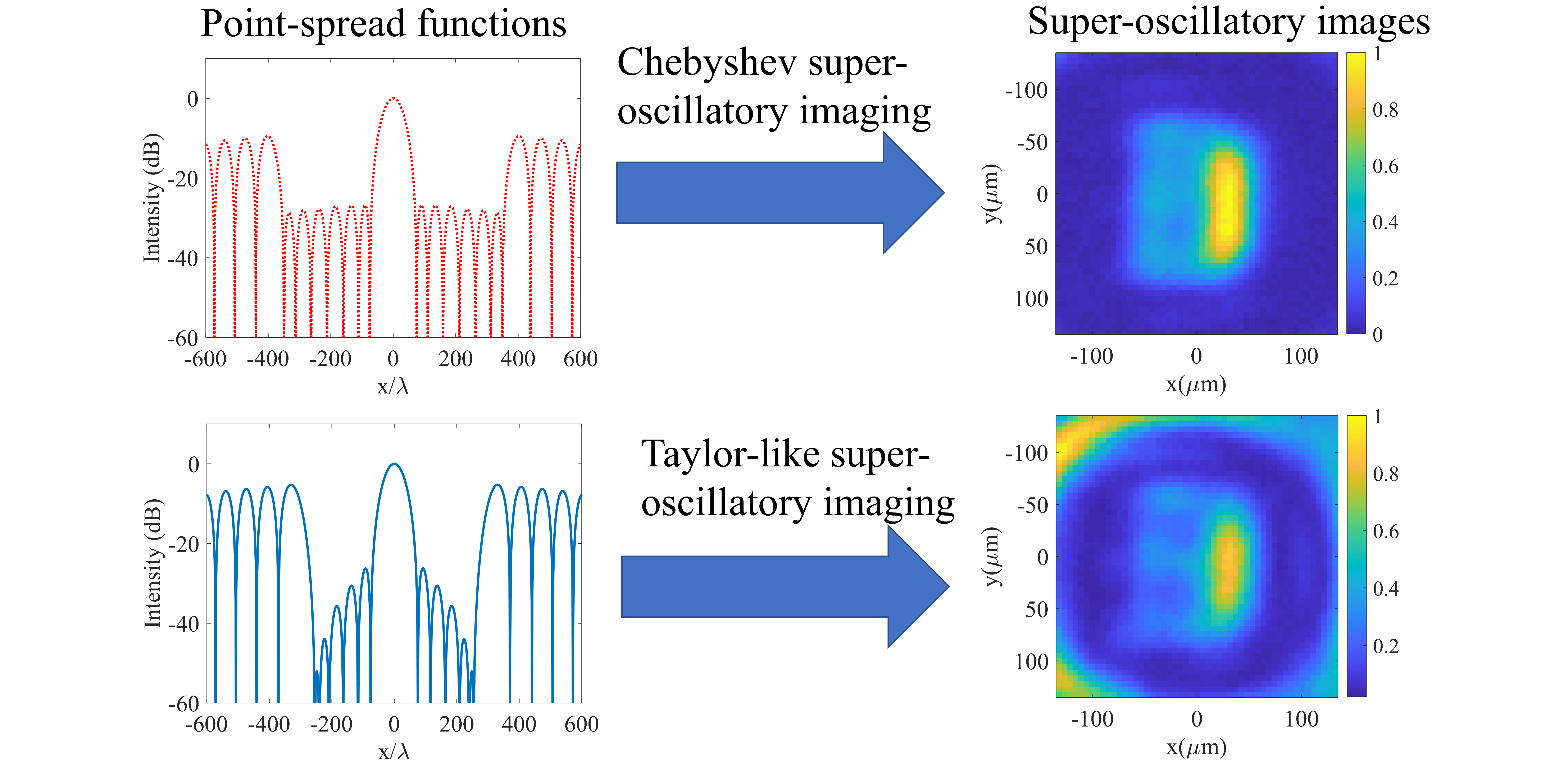It has been proved [9,10] that the intensity of the sidebands increases exponentially with the number of super-oscillations (corresponding to enlarging the ROI or reducing the main beamwidth) and polynomially with the frequency of super-oscillations, which is the number of full super-oscillations in one time or length unit (corresponding to decreasing the sidelobe level inside the ROI). When the energy contained in the sidebands becomes enormous, it is hard for detectors, such as a CMOS camera, to capture the images because the rest of the energy inside the ROI would be lower than the dynamic range threshold of the image sensor. One way to resolve this issue in a single-capture imaging apparatus [11] is to achieve a balance between the sidelobe level and the main beamwidth to keep the sideband intensity at an acceptable level. Previous synthesis of super-oscillatory point-spread functions used the Chebyshev polynomial pattern where all sidelobe levels are equal [8,11,12,13]. In this contribution, we explore the possibility and potential advantages of synthesizing super-oscillatory patterns that have tapered sidelobes. Such a sidelobe structure could mitigate the interference from sidelobes. Sidelobe suppression (including super-oscillatory sidelobes) is important for improving the resolution [13], decreasing spurious images in Optical Coherence Tomography [14], removing ambiguity in 3D imaging [15], enabling the deployment of high quality laser lithography [16] and so forth.

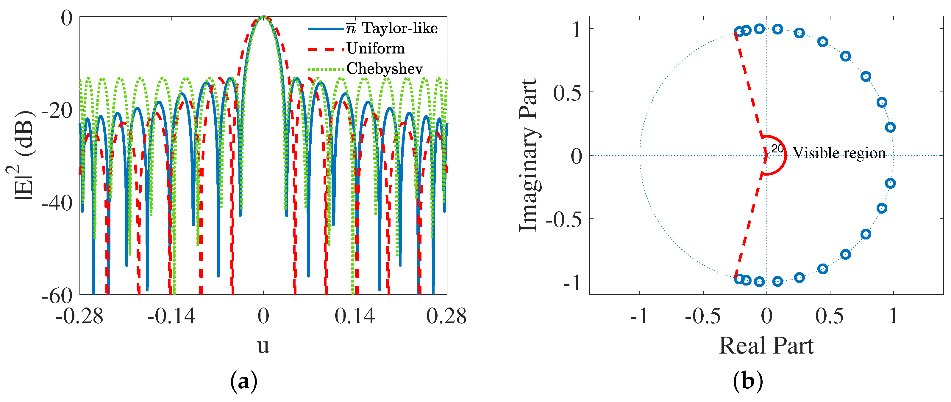
The Chebyshev super-oscillatory antenna pattern in [8] is inspired by the systematic approach derived from Chebyshev polynomials to construct super-directive patterns having uniform sidelobes [17,18,19] and the pioneering approach to the synthesis of super-directive patterns proposed by Schelkunoff [20]. This approach utilized the polynomial method and places more zeros in the visible region on the complex unit circle. By constraining the distance between a pair of zeros around the main beam and decreasing the spacing between the antenna elements, the directivity could be increased beyond that of a uniformly excited array. Although it is quite effective to achieve a narrow main beamwidth using Schelkunoff’s polynomial method, the way to control the sidelobes was not thoroughly illustrated with methods other than the use of Chebyshev and Legendre polynomials [21]. By resorting to the Taylor’s antenna pattern function [22] and Schelkunoff’s polynomial method, it is possible to sythesize the super-directive pattern with a tapered sidelobe structure. This Taylor-like super-directive pattern can then be used to extrapolate to the 2D super-oscillatory point-spread function with tapered sidelobes.

This work contributes to describing how to generate super-oscillatory patterns with tapered sidelobes based on the popular Taylor’s antenna patterns [22] and apply them for optical super-resolution imaging. In Section 1, we describe a type of transformation based on which a finite number of zeros (larger than 1) of $\overline{n}$ and one-parameter Taylor-pattern functions could be adjusted to be placed on the complex unit circle without deforming the sidelobe structure. In Section 2, a linear transformation is applied to make the visible region have a customized size to obtain super-directivity. In Section 3, we place extra zeros into the invisible region to reduce the restored energy in the near-field for super-directive antennas, which correspondingly can decrease the sideband intensity for super-oscillatory point-spread functions. In Section 4, by utilizing the fact that super-directivity in the angular domain and super-oscillation in the spatial domain are dual phenomena to each other, we extrapolate from the Taylor-like super-directive pattern to the 2D Taylor-like super-oscillatory point-spread function. Subsequently we then present several experiments with 632.8 nm laser light and a LCOS (liquid crystal on silicon) spatial light modulator (SLM) working as a programmable grating (both on phase and amplitude) to demonstrate the imaging superiority of the Taylor-like super-oscillatory point-spread function over the Chebyshev one in resolving the objects of two apertures and of a mask with the letter E.

2. Theoretical Foundation

The array factor of an array composed of N elements is given by

$$F\left(u\right)=\sum _{n=1}^N{c}_n{e}^{j2\pi (n-1)u}$$

(1)

where $u=\frac{d}{\lambda }(cos\theta -cos{\theta }_0)$, d is the element spacing of the antenna array and $c_n$ are current weights and the maximum radiation happens at ${\theta }_0$. Without loss of generality, we choose ${\theta }_0=\pi /2$ for broadside radiation. Let $z=e^{j2\pi u}$, then we have

$$F\left(u\right)=\sum _{n=1}^N{c}_n{z}^{n-1}=c_N\prod _{n=1}^{N-1}(z-z_n)$$

(2)

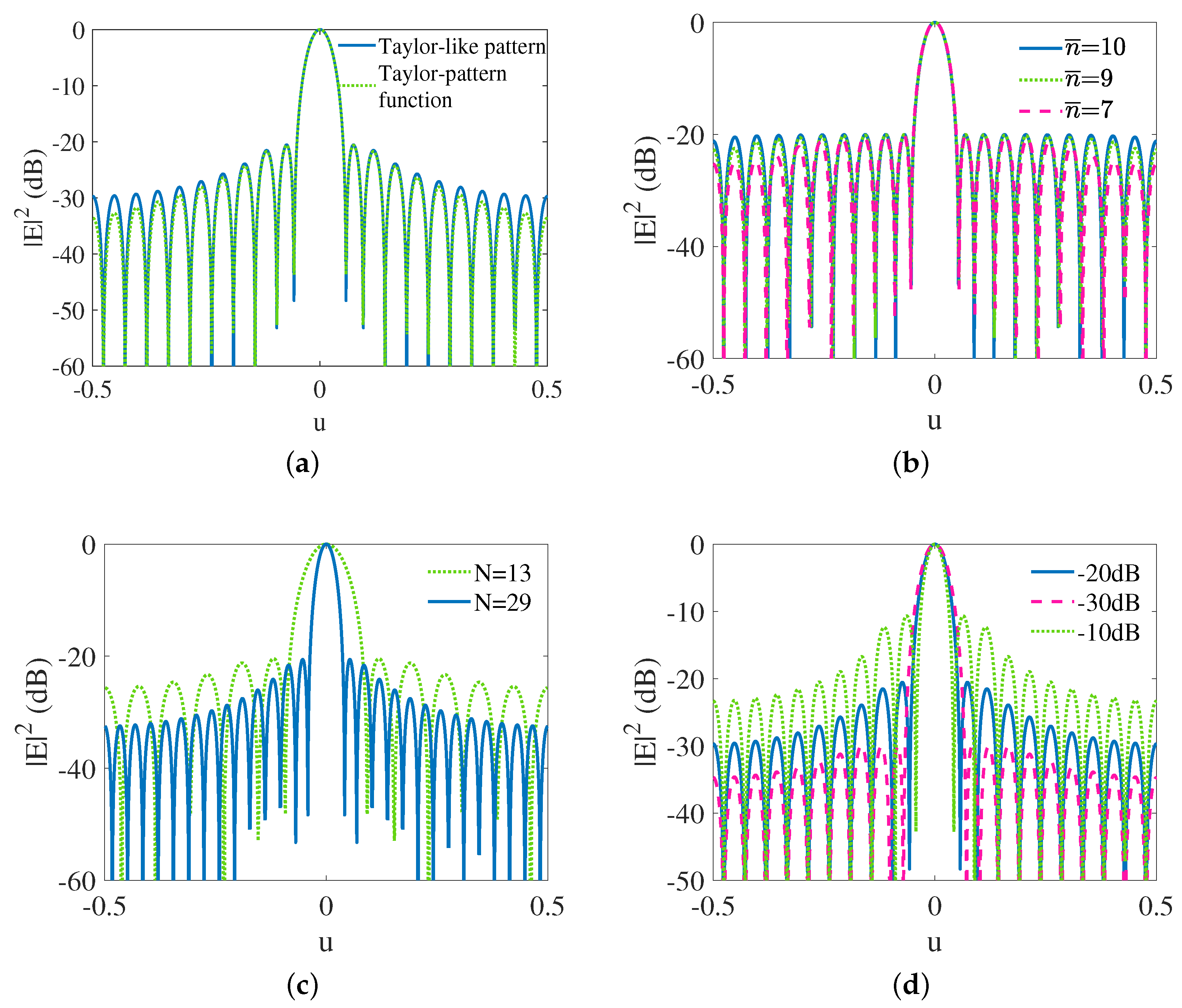
where $z_n$ are zeros on the complex unit circle. The zeros of the Chebyshev pattern are calculated in [17]. However, the problem of achieving Taylor super-directive patterns is that infinite zeros have to reside on the complex unit circle to produce such a pattern with tapered sidelobes. Moreover, the zeros of the Taylor-pattern function are not naturally limited within (−1,1), which means that a suitable transformation is needed. The $\overline{n}$ Taylor-pattern function is given by [22],

$$F_1\left(\theta \right)=\frac{sin\pi p}{\pi p}\prod _{n=1}^{\overline{n}-1}\frac{1-p^2/p_n^2}{1-p^2/n^2}$$

(3)

where $p=\frac{l}{\lambda }cos\theta$ (l is the array size), $p_n$ are the zeros, and $\overline{n}-1$ is the number of zeros inside the central region(uniform-sidelobe region). The zeros inside the central region are the zeros of the Dolph-Chebyshev array distribution multiplied by a dilation factor $\sigma$, given by [22],

$$p_n=\pm \sigma \sqrt{A^2+{(n-\frac{1}{2})}^2}1\le n<\overline{n}$$

(4)

$$p_n=\pm n\overline{n}\le n$$

(5)

where $cosh\pi A$ is the intensity ratio of the main lobe to the first sidelobe. The dilation factor is given by [23]

$$\sigma =\frac{\overline{n}}{\sqrt{A^2+{(\overline{n}-\frac{1}{2})}^2}}$$

(6)

Theoretically, inside the central region, the sidelobes should be uniform and outside the central region, the sidelobes should be taperd asymptotically to $\frac{sin\left(\pi p\right)}{\pi p}$ with a pedestal. In reality however, the sidelobes inside the central region would be slighly tapered because the dilation factor $\sigma$ is slightly larger than 1. Therefore, the Taylor pattern could be recognized as a pattern with a narrow beamwidth and tapered sidelobes.

The one-parameter Taylor-pattern function is given by [24]

$$\begin{array}{c}\hfill F_2\left(\theta \right)=\left\{\begin{array}{cc}l\frac{sinh\left[\pi \sqrt{B^2-p^2}\right]}{\pi \sqrt{B^2-p^2}}\hfill & p^2<B^2\hfill \\ l\frac{sin\left[\pi \sqrt{p^2-B^2}\right]}{\pi \sqrt{p^2-B^2}}\hfill & p^2>B^2\hfill \end{array}\right.\end{array}$$

(7)

where B is a constant to determine the first sidelobe level calculated through solving $R_0=4.603\frac{sinh\left(\pi B\right)}{\pi B}$ where $R_0$ is the intensity ratio of the main lobe to the first sidelobe. The zeros could be given by

$$p_n=\sqrt{B^2+n^2};$$

(8)

Tseng [25] has made an effort to map the zeros of the Taylor-pattern function to a set belonging to (0,1) by setting ${\gamma }_n=cos\left(\frac{p_n\pi }{N}\right)$. In this approach, an effective way to achieve a Taylor pattern for a line source with a deep null is implemented by using $F\left({\zeta }_1\right)={\prod }_{n=1}^{\frac{N-1}{2}}\frac{{\zeta }_1^2-{\gamma }_n^2}{1-{\gamma }_n^2}$, where ${\zeta }_1=cos\pi u$ and N is an odd number. We found that by making ${\gamma }_n^{{}^{\prime }}=cos\left(\frac{2p_n\pi }{N}\right)$, the transformed zeros ${\gamma }_n^{{}^{\prime }}$ could be used in ${\prod }_{n=1}^{\frac{N-1}{2}}\frac{{\zeta }_2-{\gamma }_n^{{}^{\prime }}}{1-{\gamma }_n^{{}^{\prime }}}$, where ${\zeta }_2=cos2\pi u$, to produce a pattern the same as $F\left({\zeta }_1\right)$. In this way, the Schelkunoff’s polynomial method could be applied by resorting to ${\gamma }_n^{{}^{\prime }}$. The first transformation process of zeros is given below

$${\beta }_n=e^{j\left(\frac{2p_n\pi }{N}\right)}$$

(9)

$$F\left(u\right)=\prod _{n=1}^{\frac{N-1}{2}}(z-{\beta }_n)(z-{\beta }_n^{*})$$

(10)

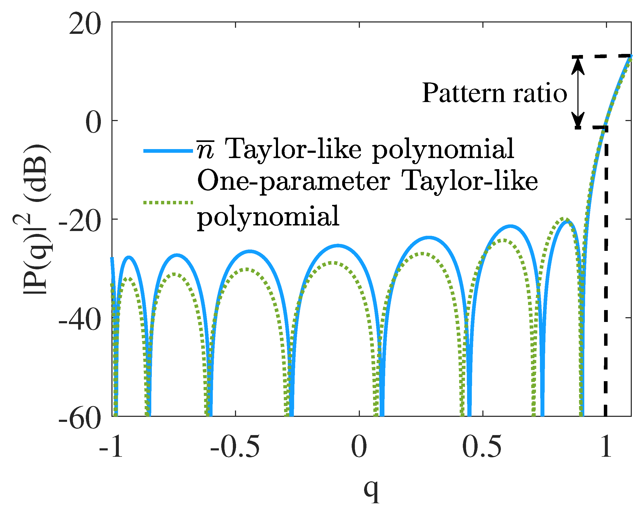
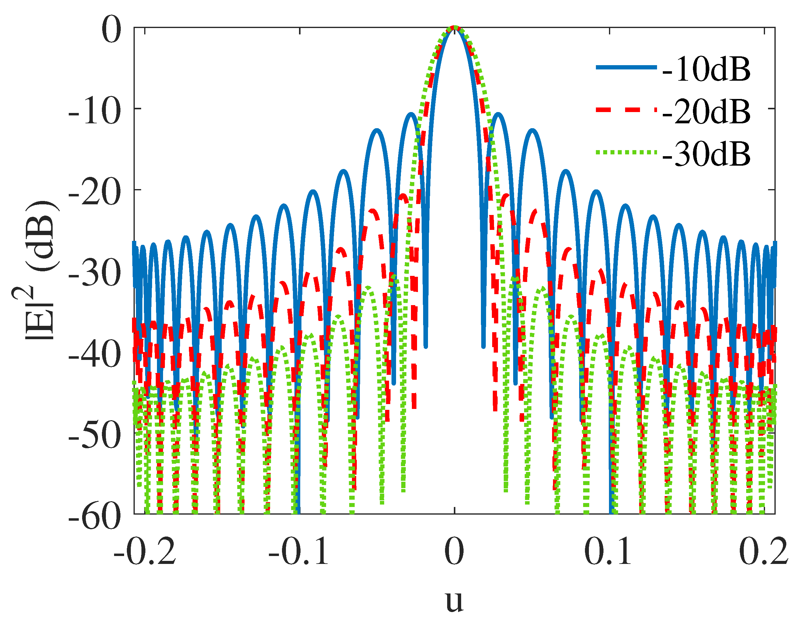
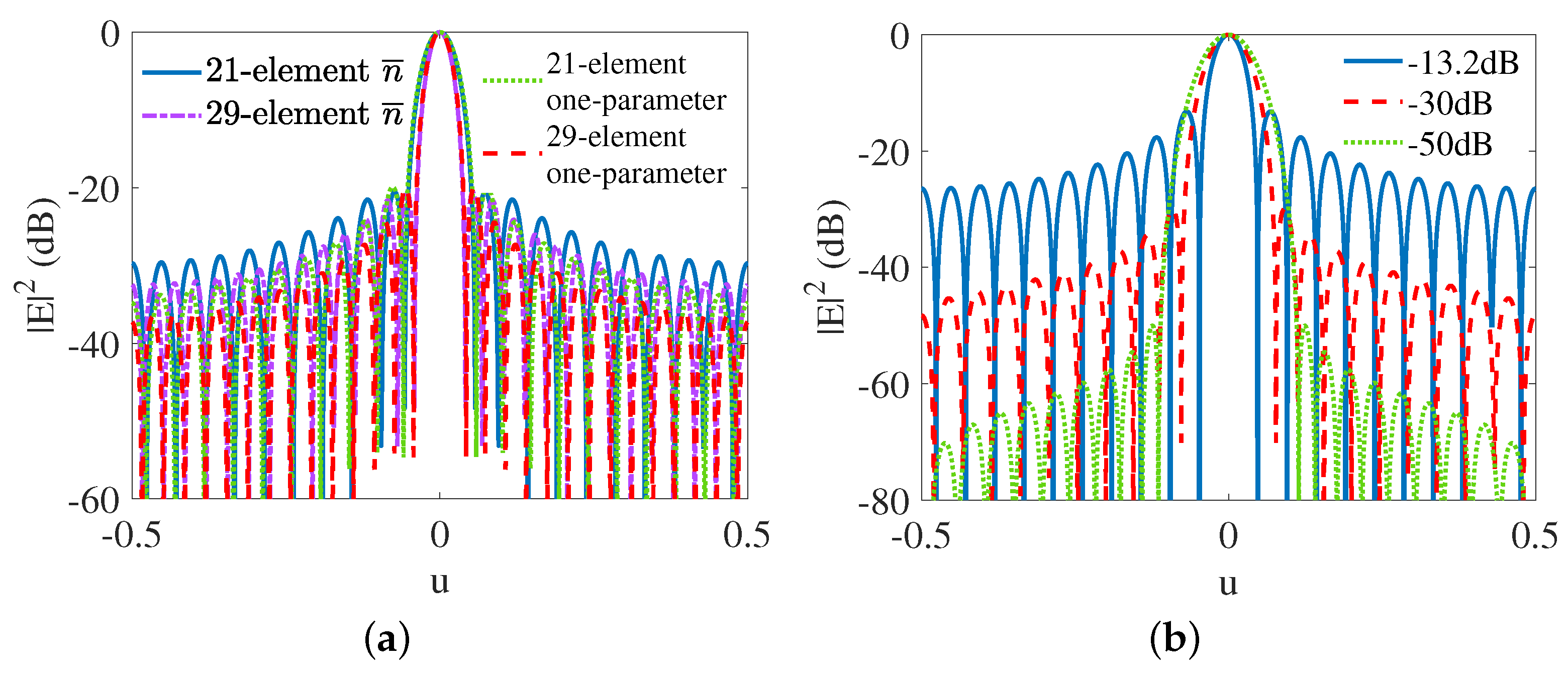
where ${\beta }_n$ are transformed zeros on the complex unit circle from the zeros of the Taylor-pattern functions and ${\beta }_n^{*}$ is the conjugate of ${\beta }_n$. It is shown in Figure 1 that by using Schelkunoff’s polynomial method, the $\overline{n}$ and the one-parameter Taylor-like polynomials are obtained. The difference between Chebyshev polynomials and Taylor-like polynomials is uniform sidelobes versus tapered sidelobes. A phenomenon in Figure 1a that merits some attention is that the first sidelobe level of the $\overline{n}$ Taylor-like polynomial (red line) is very close to 0 dB if $cosh\pi A=0$ dB. As is shown in Figure 1b, however, even though $B=0$, the first sidelobe level is −13.2 dB far lower than 0 dB. 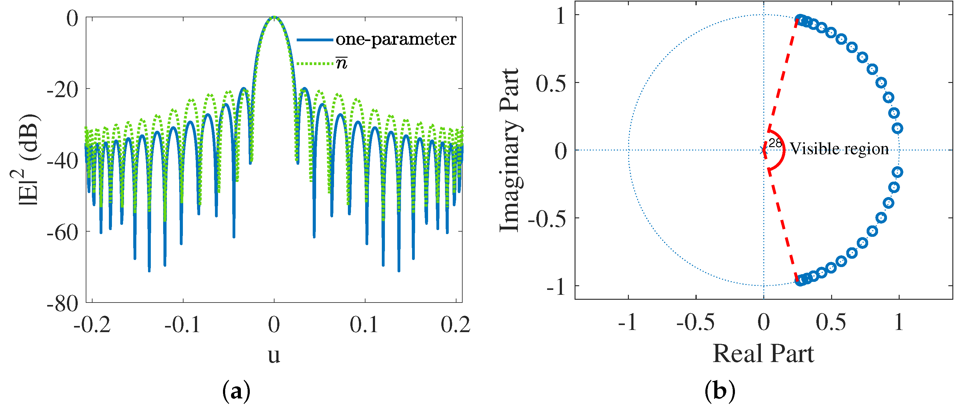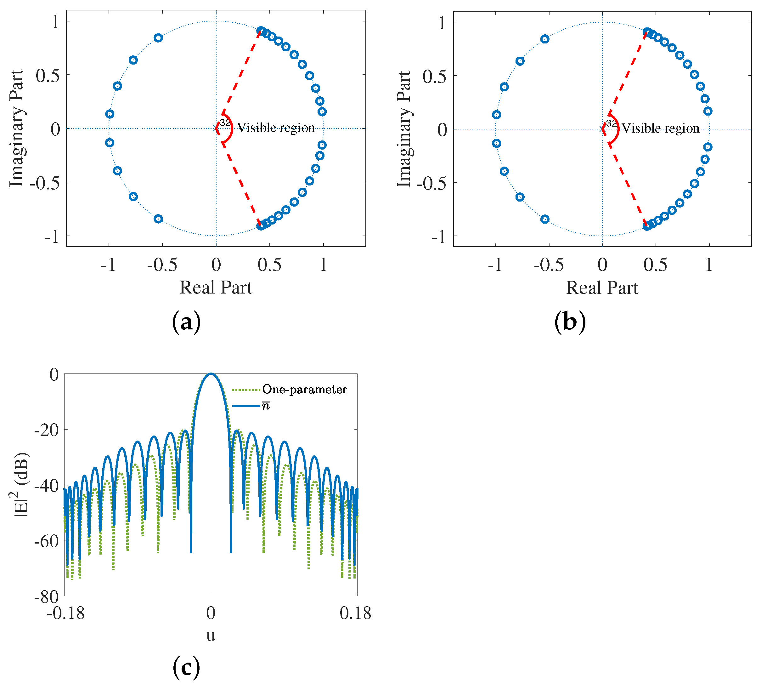This means that the control of the first sidelobe level for the one-parameter Taylor-like polynomial is not as flexible as for the $\overline{n}$ Taylor-like polynomial. The comparison of the $\overline{n}$ and one-parameter Taylor-like polynomials is shown in Figure 2 where it is clearly illustrated that the tapering rate of the sidelobes for the one-parameter Taylor-like polynomial is faster than that for the $\overline{n}$ Taylor-like polynomial.

3. Theoretical Approach to Taylor-Like Super-Directive Patterns

3.1. $\overline{n}$ Taylor-Like Super-Directive Patterns

The approach here is using a finite number of zeros of the Taylor-pattern function to produce the super-directive patterns with another transformation utilized to squeeze the visible region from the entire unit circle into a smaller size. The $\overline{n}$ Taylor-like patterns are produced as shown in Figure 3a. This Taylor-like pattern has a slightly different sidelobe structure compared to the Taylor-pattern function. The reason is that this Taylor-like pattern is achieved by using a finite number of zeros in the Schelkunoff’s polynomial but the Taylor-pattern function has an infinite number of zeros. It is shown in Figure 3b that the Taylor-like pattern is approaching a Chebyshev pattern when $\overline{n}$ is increasing to $(N-1)/2$, where N is the number of elements. This characteristic, which stems from the ideal Taylor-pattern function, is also inherent in the Taylor-like pattern. As is shown in Figure 3c, the main beamwidth becomes narrower when the number of elements is increasing. The ability to control the first sidelobe level is shown in Figure 3d. Furthermore, the linear transformation for contracting the visible region, leading to super-directivity, is given by

$${\alpha }_n=cos\left(\frac{2p_n\pi }{N}\right)$$

(11)

$$v_n=\frac{1-cos\left(R\right)}{c+1}[{\alpha }_n+\frac{1+c·cos\left(R\right)}{1-cos\left(R\right)}]$$

(12)

$$w_n=v_n+i\sqrt{1-v_n^2}$$

(13)

$$F\left(u\right)=\prod _{n=1}^{\frac{N-1}{2}}(z-w_n)(z-w_n^{*})$$

(14)

where R is half the range of the visible region and c is a constant, obtained by solving the Taylor-like polynomial given a pattern ratio, similar to the parameter for adjusting the sidelobe level of Chebyshev patterns [24,26]. It should be noted that $c=1$ corresponds to the pattern ratio of 0dB whereas the pattern ratio is defined in Figure 2. The linear transformation (12) should, to some extent, be familiar to obtaining super-directivity by adjusting the visible region since it has been used decades ago [19,26,27]. On the other hand, the transformation (11) transforms a finite number of zeros of the Taylor-pattern function onto the complex unit circle, which is the basis for the second transformation (12) to constrain the visible region.

The patterns of the Taylor super-directive, Chebyshev super-directive and uniform arrays are compared in

Table 1. Parameters of a $\overline{n}$ Taylor-like super-directive pattern.

$\mathit{N}=21$, $\overline{\mathit{n}}=3$ and $\mathit{d}=0.29\mathit{\lambda }$
	Types	Taylor	Chebyshev	Uniform
Parameters
First sidelobe level (dB)		−13.27	−13.27	−13.27
Directivity (dBi)		11.84	11.29	10.86
Half power beamwidth (DEG)		6.52	6.14	8.44
Maximum weighting ratio		1.86 × ${10}^3$	2.12 × ${10}^3$	1

. The first sidelobe level of the super-directive patterns is designed to be the same as that of the corresponding uniform array, while the directivity is greater than that of the uniform array. As studied in [19,28], the maximum weighting ratio, defined by $max\left\{\right|c_n\left|\right\}/min\left\{\right|c_n\left|\right\}$, is much greater than that of the uniform array, which is one of the well-known disadvantages of super-directive arrays. We will address this problem in Section 4.

The representative Taylor-like super-directive and Chebyshev super-directive patterns, and the reference uniform pattern are shown in Figure 4a. It is observed that the major lobe of the Taylor-like pattern is slightly wider than that of the Chebyshev pattern and both major lobes are obviously narrower than that of the reference pattern from the uniform array. In radar applications, tapered minor lobes could reduce the interference from them into the receiving antenna. It is clearly shown in Figure 4b that the visible region is contracted to $(-0.57\pi ,0.57\pi )$ down from the entire unit circle. Since the pattern ratio and $cosh\pi A$ are both able to control the first sidelobe level, we need to explore the mechanism, which is unique for Taylor-like super-directive patterns, by combining the pattern ratio and $cosh\pi A$ to adjust the first sidelobe level. It is shown in Figure 5 and

Table 2. Comparison of $\overline{n}$ Taylor-like super-directive patterns with different combinations of $cosh\pi A$ and pattern ratios.

$\mathit{d}=0.21\mathit{\lambda }$, $\overline{\mathit{n}}=3$ and $\mathit{N}=29$
	Parameters	c	Directivity (dBi)	Directivity Ratio	Maximum Weighting Ratio
Pattern Ratio (dB) and$\mathit{cosh}\mathit{\pi }\mathit{A}$
4 dB and 6 dB		1.01	12.89	1.59	$1.57\times {10}^6$
12 dB and 8 dB		1.02	12.68	1.52	$1.53\times {10}^6$
15 dB and 15 dB		1.03	12.09	1.32	$1.50\times {10}^6$

that the combination of the pattern ratio and $cosh\pi A$ could give us more freedom to control the first sidelobe level. For instance, we are able to achieve the −30dB first sidelobe level without a limit on $\overline{n}$, which is inherently a drawback in the Taylor-pattern function (e.g., the condition $\overline{n}=3$ is not suitable for first sidelobe levels lower than −25 dB [22]).

3.2. One-Parameter Taylor-Like Super-Directive Patterns

A one-parameter Taylor-like polynomial could offer a faster tapering rate of the sidelobes than the commensurate $\overline{n}$ Taylor-like polynomial. Hence, it is a worthy effort to pursue the one-parameter approach to produce super-directive patterns with tapered sidelobes. As is shown in Figure 6a, either for the 21-element or for the 29-element one-parameter Taylor-like pattern, the sidelobes are tapering faster than their counterparts for the $\overline{n}$ Taylor-like patterns with the preset $R_0$ equal to 20 dB. The 29-element $\overline{n}$ Taylor-like pattern almost has the same tapering rate as the 21-element one-parameter Taylor-like pattern. The adjustability of the first sidelobe level for the one-parameter Taylor-like patterns is illustrated in Figure 6b where the blue line denotes the pattern with the highest first sidelobe level which is −13.2 dB, the same as that in $sinu/u$.

The one-parameter Taylor-like super-directive pattern is compared with the $\overline{n}$ type in Figure 7a where the former one is tapering faster than the latter, which is consistent with what was mentioned in Figure 6a. The corresponding zeros distribution is shown in Figure 7b. The parameters for both the one-parameter and the $\overline{n}$ Taylor-like patterns are given in

Table 3. Comparison of the two types of Taylor-like super-directive patterns.

$\mathit{N}=29$ and $\mathit{d}=0.21\mathit{\lambda }$
	Types	One-Parameter	$\overline{\mathit{n}}$
Parameters
First sidelobe level (dB)		−20	−20
Directivity (dBi)		12.69	12.84
Half power beamwidth (DEG)		5.92	5.54
Maximum weighting ratio		1.54 × ${10}^6$	1.56 × ${10}^6$

in which we draw the conclusion that although the tapering rate of the one-parameter Taylor-like pattern is faster than that of the $\overline{n}$ type, the main beamwidth for the $\overline{n}$ type is actually narrower. This is the reason why the directivity of the $\overline{n}$ Taylor-like super-directive pattern is slightly higher than the one-parameter type.

4. Reduction of the Maximum Excitation Weighting Ratio

One of the most severe issues of putting super-directive arrays into practice is the required huge maximum excitation weighting ratios. We found that by adding zeros in the invisible region on the complex unit circle we could decrease the maximum excitation weighting ratio considerably. As is well-known, there is a great amount of reactive energy in the near-field because the electromagnetic waves are not propagating in the longitudinal direction. Hence, the wavenumber $k_z$ is imaginary whereas the transverse wavenumber $k_t$ is larger than $2\pi /\lambda$. This means that the z (which is $e^{j2\pi u}$) in the array factor of the polynomial migrates into the invisible region. If there exists no zeros in the invisible region, the reactive energy would increase polynomially with the the wavenumber $k_t$ increasing. However, by adding zeros in the invisible region, this polynomially increasing reactive energy will become oscillating, which means that the total reactive energy would be reduced. Then there is no need for the maximum ratio of element weights to be extremely large. As shown in Figure 8a,b, there are extra zeros outside the visible region. The exact maximum weighting ratio decreases from almost $5.8\times {10}^4$ to 464, as shown in

Table 4. Comparison of the two types of Taylor-like super-directive patterns with reduced maximum weighting ratio.

$\mathit{N}=33$ with 8 Extra Zeros Outside the Visible Region or $\mathit{N}=25$ without Extra Zeros
	Types	One-Parameter ($\mathit{N}=\mathbf{33}$)	$\overline{\mathit{n}}$($\mathit{N}=\mathbf{33}$)	One-Parameter ($\mathit{N}=\mathbf{25}$)	$\overline{\mathit{n}}$($\mathit{N}=\mathbf{25}$)
Parameters
d		0.18$\lambda$	0.18$\lambda$	0.24$\lambda$	0.24$\lambda$
Array size		5.82$\lambda$	5.82$\lambda$	5.76$\lambda$	5.76$\lambda$
First sidelobe level (dB)		−20	−20	−20	−20
Directivity (dBi)		12.27	12.02	12.34	12.16
Directivity ratio		1.38	1.30	1.40	1.34
Maximum weighting ratio		478.15	464.00	$6.05\times {10}^4$	$5.80\times {10}^4$

with the trade-off being the reduction of the element spacing. The corresponding patterns are shown in Figure 8c where different tapering rates could be observed.

5. Imaging Theory and Experimental Results

In this section, we first summarize the duality between super-directivity in the angular domain and super-oscillation in the spatial domain [8]. Based on this duality, we obtain the 1-D super-oscillatory point-spread function. Then, we extrapolate from 1-D super-oscillatory point-spread functions to 2-D super-oscillatory point-spread functions [11]. Since the super-oscillatory phase mask is displayed on an SLM as a grating, we hereby derive the point-spread functions for every diffraction order on the image plane. The first order is chosen to implement the super-oscillatory experiments instead of the zeroth order because of the limitation of the diffraction efficiency of the SLM [29]. Finally, through experiments, we demonstrate the superiority of the Taylor-like super-oscillatory point-spread functions over the Chebyshev ones in resolving the objects of two apertures and of a mask with the letter E.

To explain this duality, one of the details is that the polynomial of both super-directivity and super-oscillation can both be given by

$$G=\sum _{n=1}^N{c}_n{z}^{n-1}$$

(15)

where $z=e^{jkdcos\theta }$ for super-directivity and $z=e^{j\mathsf{\Delta }kx}$ for super-oscillation. For super-directivity, this polynomial achieves the transformation from the spatial domain ($nd$) to the angular domain ($\theta$). For super-oscillation, this polynomial achieves the transformation from the k domain ($n\mathsf{\Delta }k$) to the spatial domain (x). 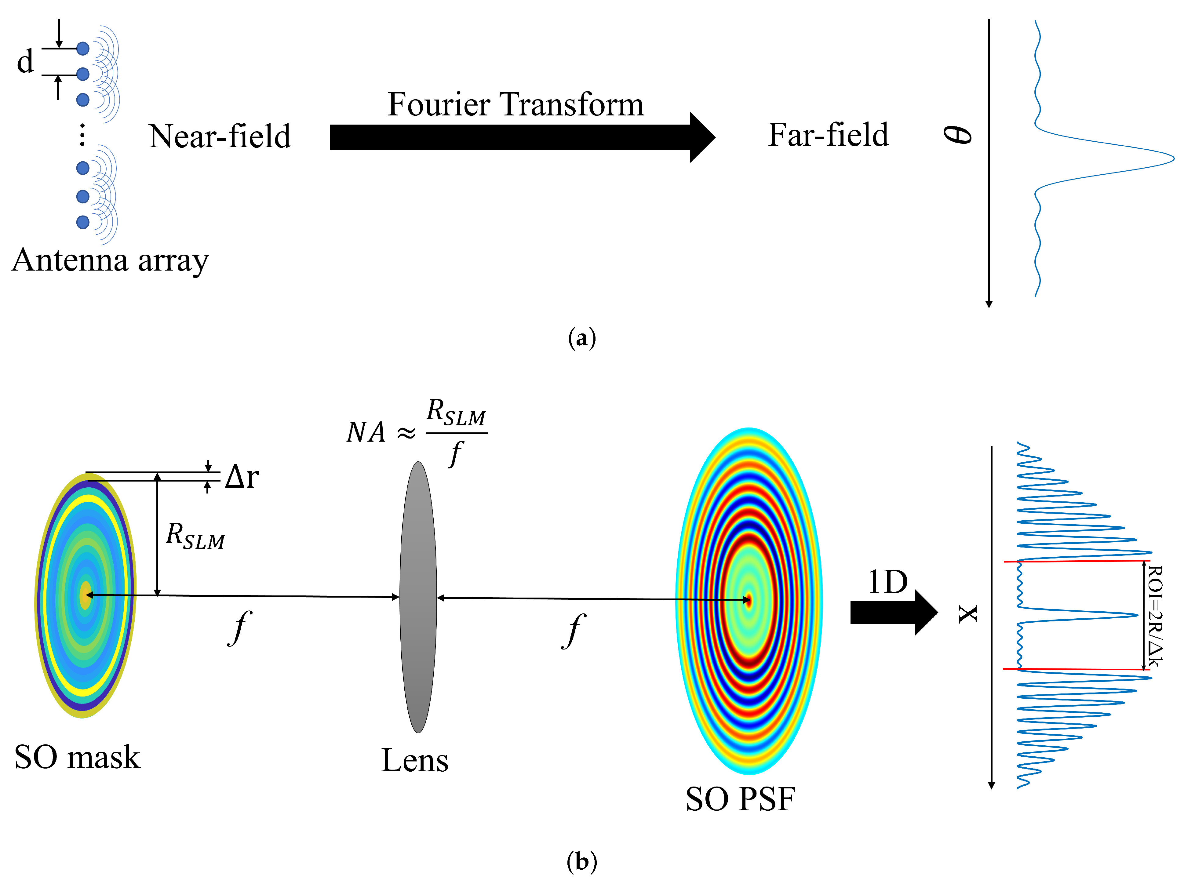Since there is no bound for x, there exists no ’invisible’ region for super-oscillation, which means that the counterpart to the reactive energy in the near-field of super-directive antennas is observable in super-oscillations. The detail of transforming from $z=e^{jkdcos\theta }$ to $z=e^{j\mathsf{\Delta }kx}$ in an optical scenario regarding the numerical aperture (NA) of the imaging lens is given by

$$z=e^{jkdcos\theta }=e^{j\frac{2k·NA}{M}\frac{Mdcos\theta }{2NA}}=e^{j\mathsf{\Delta }kx}$$

(16)

where M is the number of frequency samples on the Fourier plane, which is $(N+1)/2$, and d can be calculated by $R·\lambda /2\pi$ where R is half the pre-determined visible region in (12). The diagram to illustrate this transformation is shown in Figure 9.

Since we have already obtained the zeros on the complex unit circle for the Taylor-like super-directive patterns, we can easily get the Taylor-like super-oscillatory point-spread function by

$$f\left(x\right)=c_N\prod _{n=1}^{N-1}(z-z_n)$$

(17)

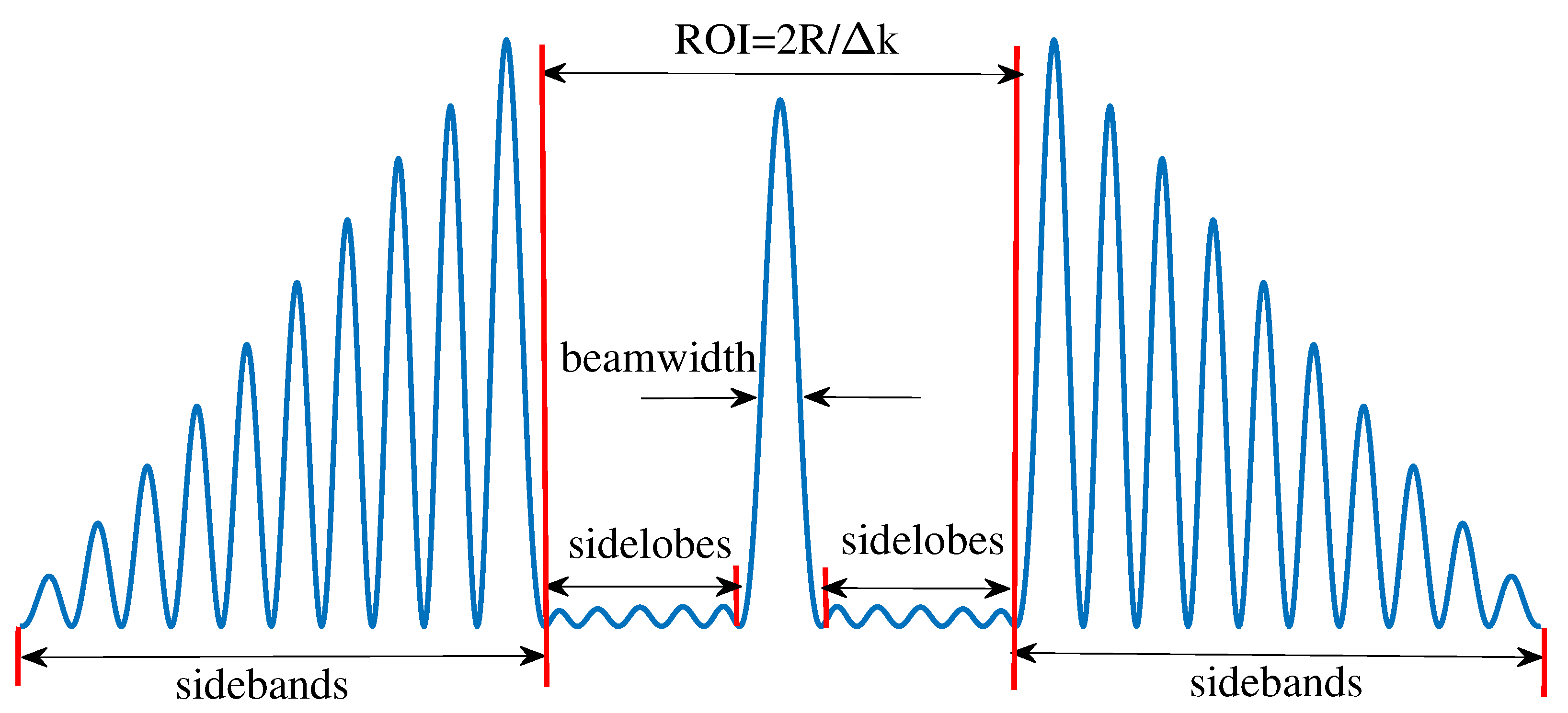
where $z_n$ are the zeros on the complex unit circle and $z=e^{j\mathsf{\Delta }kx}$. The technique for reducing the maximum excitation weighting ratio in Section 4 has also been utilized here to suppress the intensity of the sidebands [30,31], which is available in that the sidebands in the super-oscillatory point-spread functions and reactive fields in the super-directivity antennas are dual counterparts to each other. A diagram for an example of the 1-D super-oscillatory point-spread function is shown in Figure 10.

The way to extrapolate the 1-D super-oscillatory point-spread function to its 2-D counterpart is chosen to be

$$f\left(r\right)=\sum _{m=1}^M{a}_m{k}_{{\rho }_m}{J}_0\left(k_{{\rho }_m}r\right)$$

(18)

where $a_n$ is a coefficient, $J_0$ is the Bessel function of the first kind of order zero, $k_{{\rho }_m}$ is the radial component in the $(k_{\rho },k_{\theta })$ domain, and $f\left(r\right)$ is the 2-D point-spread function by replacing the variable x in (17) with r in polar coordinates. We basically use a set of orthogonal Bessel functions to fit the designed super-oscillatory point-spread function. The specific method used for fitting is the zero matching method given by [11]

$$f\left(x_n\right)=\sum _{m=1}^M{a}_m{k}_{{\rho }_m}{J}_0\left(k_{{\rho }_m}{x}_n\right)=0$$

(19)

where $x_n=arg\left[z_n\right]/\mathsf{\Delta }k$ for $n=(N-1)/2+1$ to $N-1$, ranked in an ascending order, $z_n$ are the zeros on the complex plane, and $arg\left[z_n\right]$ are the phases of $z_n$. The matrix form of (19) is $\tilde{\mathit{J}}\tilde{\mathit{A}}=\left[\mathbf{0}\right]$ where $\tilde{\mathit{J}}$ is a $(N-1)/2\times M$ matrix whose elements are $k_{{\rho }_m}{J}_0\left(k_{{\rho }_m}{x}_n\right)$, $\tilde{\mathit{A}}$ is the coefficient matrix, and the $\left[\mathbf{0}\right]$ is the zero matrix. Then the solved coefficients in $\tilde{\mathit{A}}$ are assigned to pixels on the SLM according to the Hankel transform given by

$$F\left(k_{\rho }\right)=2\pi {\int }_0^{\infty }f\left(r\right)J_0\left(k_{\rho }r\right)rdr$$

(20)

where $F\left(k_{\rho }\right)$ is the optical transfer function. This expression holds because the SLM in the experiment modulates the optical transfer function on the Fourier plane. After substituting (18) for the $f\left(r\right)$ in (20), we obtain

$$\begin{array}{cc}\hfill F\left(k_{\rho }\right)& =2\pi \sum _{m=1}^M{a}_m{k}_{{\rho }_m}{\int }_0^{\infty }{J}_0\left(k_{{\rho }_m}r\right)J_0\left(k_{\rho }r\right)rdr\hfill \\ \hfill & =2\pi \sum _{m=1}^M{a}_m\delta (k_{\rho }-k_{{\rho }_m})\hfill \end{array}$$

(21)

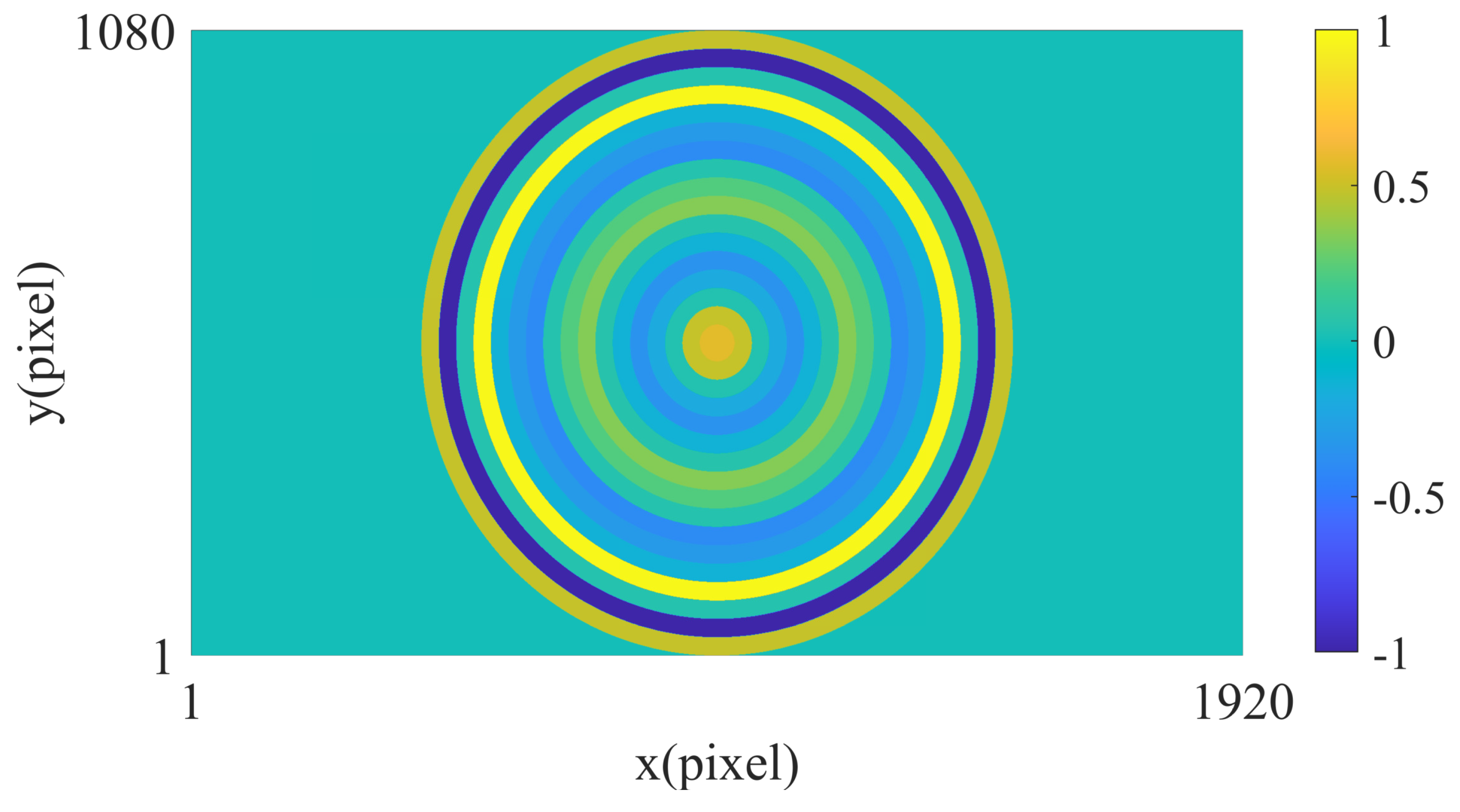
It is apparent that $F\left(k_{\rho }\right)$ contains M rings, each of which has a specific coefficient. In our experiment, the simulated $F\left(k_{\rho }\right)$ to be mapped onto the SLM is shown in Figure 11. The width $\mathsf{\Delta }r$ of each ring is determined by

$$\mathsf{\Delta }r=\frac{D_{SLM}}{2M-1}$$

(22)

where $D_{SLM}$ is 6.9mm, the diameter of the SO mask and $M=17$, the total number of coefficients. The phase-only SLM that we used has $1920\times 1080$ pixels with a pitch of 6.4 $\mathsf{\mu }$m and an active area of $12.5\times 7.1$ mm${}^2$. Based on the fact that the pixel pitch is ten times larger than the red-laser wavelength and the modulation is only applied to a specific polarization, the SLM functions the same as a programmable grating that can modulate both the phase and amplitude of the optical field. To make our phase-only SLM capable of amplitude modulation, the technique of super-pixelling is utilized [32]. The intuitive way to explain this is that two unit complex vectors on the whole complex plane (equivalent to the $2\pi$ phase modulation of this SLM) can be combined with varying phase difference to obtain any complex coefficients, mathematically given by,

$$e^{j{\theta }_1}+e^{j{\theta }_2}=a_m$$

(23)

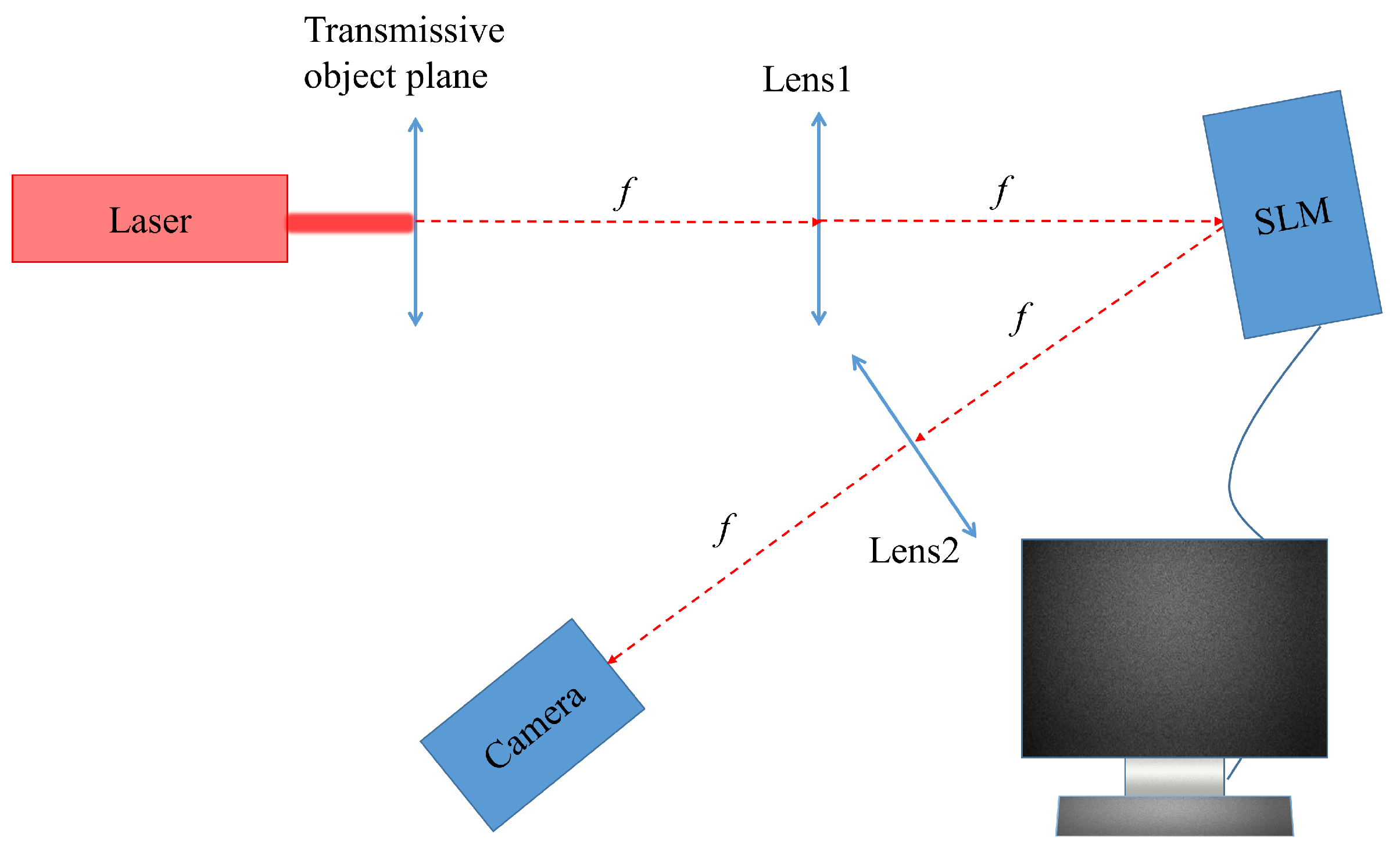
where ${\theta }_1$ and ${\theta }_2$ are the modulated phases on the SLM by the host computer, and $a_m$ is the normalized coefficient in (21). The entire experiment is conducted in an optical 4F system (as shown in Figure 12) with this reflective SLM standing on the Fourier plane [11]. The imaging process in this system is expressed by

$$f_{img}=IFT\left[F\left(k_{\rho }\right)FT\left[f_{obj}\right]\right]$$

(24)

where $f_{img}$ is the image function, $f_{obj}$ is the object function, $F\left(k_{\rho }\right)$ is the optical transfer function in (21) to be mapped onto the SLM, $FT[•]$ denotes the Fourier transform implemented by the objective lens and $IFT[•]$ denotes the inverse Fourier transform implemented by the imaging lens.

The derivation of the whole point-spread function $h(x,y)$ including all the diffraction orders on the image plane is given in Appendix A. Since the $h(x,y)$ is complex, let us focus on the zeroth diffraction order and the first diffraction order. The components of the zeroth diffraction order can be given by

$$f_1(x,y)=\frac{w^3}{2}\sum _{m=1}^M(R_{1_m}+R_{2_m}{e}^{j\varphi })J_0\left(k_{{\rho }_m}\sqrt{x^2+y^2}\right)$$

(25)

$$\begin{array}{c}\hfill f_2(x,y)=w\sum _{\genfrac{}{}{0pt}{}{n_1=-K}{n_1\ne 0}}^K\left\{\frac{j}{4n_1^2{\pi }^2}(1-cos\left(2\pi n_{1}w\right))\sum _{m=1}^M(R_{1_m}+R_{2_m}{e}^{j\varphi })J_0\left(k_{{\rho }_m}\sqrt{x^2+y^2}\right)\right\}\end{array}$$

(26)

where $f_1$ is extracted from $h_1$ and $f_2$ is extracted from $h_2$ (see Appendix A). The first diffraction order along the x-axis can be given by

$$\begin{array}{c}\hfill g_1(x,y)=\frac{-j{w}^2}{\pm 2\pi }(e^{\pm jw\pi }-1)\sum _{m=1}^M(R_{1_m}-R_{2_m}{e}^{j\varphi })J_0\left(k_{{\rho }_m}\sqrt{{(x\pm \frac{\lambda f}{p})}^2+y^2}\right)\end{array}$$

(27)

$$\begin{array}{cc}\hfill g_2(x,y)=& w\sum _{\genfrac{}{}{0pt}{}{n_1=-K}{n_1\ne 0}}^K\left\{\frac{-1}{4n_1(-2n_1\pm 1){\pi }^2}(e^{-j{n}_{1}2\pi w}-1)(e^{-j(-2n_1\pm 1)w\pi }-1)·\right.\hfill \\ & \sum _{m=1}^M\left.(R_{1_m}-R_{2_m}{e}^{j\varphi })J_0(k_{{\rho }_m}\sqrt{{(x\pm \frac{\lambda f}{p})}^2+y^2})\right\}\hfill \end{array}$$

(28)

where $g_1$ is extracted from $h_1$ and $g_2$ is extracted from $h_2$ (see Appendix A). Therefore, the coefficients $a_m$ for the zeroth and first diffraction orders can be given by

$$\left\{\begin{array}{ccc}{a}_{0_m}=R_{1_m}+R_{2_m}{e}^{j\varphi }\hfill & \mathrm{where}& f_{SO}=C_0\sum _{m=1}^M(R_{1_m}+R_{2_m}{e}^{j\varphi })J_0\left(k_{{\rho }_m}\sqrt{x^2+y^2}\right)\hfill \\ a_{1_m}=R_{1_m}-R_{2_m}{e}^{j\varphi }\hfill & \mathrm{where}& f_{SO}=C_1\sum _{m=1}^M(R_{1_m}-R_{2_m}{e}^{j\varphi })J_0\left(k_{{\rho }_m}\sqrt{{(x\pm \frac{\lambda f}{p})}^2+y^2}\right)\hfill \end{array}\right.$$

(29)

where $f_{SO}$ is the super-oscillatory point-spread function, $C_0$ and $C_1$ are complex constants.

The distance $D_x$ between two neighboring diffraction orders along the x-axis is $\lambda f/p$ which can be obtained in another way through the grating function by

$$tan{\theta }_m\approx {\theta }_m\approx sin{\theta }_m=\lambda /p$$

(30)

$$D_x=f·tan{\theta }_m$$

(31)

where f is the focal length. The distance $D_y$ between two neighboring diffraction orders along the y-axis is $2\lambda f/p$.

By looking into (29), we can conclude that

$$a_{1_m}=R_{1_m}-R_{2_m}{e}^{j\varphi }=R_{1_m}+R_{2_m}{e}^{j(\pi +\varphi )}$$

(32)

Thus, an extra $\pi$ phase shift needs to be taken into consideration when designing the super-pixel modulations for the first diffraction order. Because of the high dynamic range of the modulations for achieving super-oscillatory fields, some coefficients after normalization are close to zero. However, it is hard to achieve such coefficients in the zeroth diffraction order due to the limitation of the diffraction efficiency of the SLM [29]. Consequently, we choose to observe the super-oscillatory patterns at the first diffraction order. Therefore the following imaging results are all captured at the first diffraction order.

We design two different Taylor-like super-oscillatory point-spread functions for two types of experiments. One Taylor-like super-oscillatory point-spread function is prepared for the point-spread function measurement to showcase the sub-diffraction main beam and tapered sidelobes (See Figure 13). The other is designed to have the same main beamwidth as the diffraction-limited one to highlight the resolution improvement only from the tapered sidelobes (See Figure 14 and Figure 15). As is shown in Figure 13a, the experimental two dimensional Taylor-like super-oscillatory point-spread function is plotted where the circular dark area corresponds to the visible region of a two-dimensional Taylor-like super-directive array. The bright dot inside the center of the visible region is the main beam and those dim circles around this dot are all the sidelobes. The bright circles outside of the central dark area, called sidebands, are the counterpart of the non-observable reactive fields in antenna super-directivity patterns. In Figure 13b, the experimental one-dimensional intensity distributions of the Taylor-like super-oscillatory point-spread function and the diffraction-limited point-spread function (corresponding to the uniform array $sinc\left(\mathrm{NA}{k}_{0}x\right)$ pattern, where NA is the numerical aperture of the imaging lens and $k_0$ is the wave number in free space) at the $y=0$ plane are obtained. This Taylor-like super-oscillatory point-spread function has tapered sidelobes and a narrower main beamwidth compared to the diffraction-limited point-spread function. The full widths at half maximum (FWHM) for the experimental and theoretical Taylor-like super-oscillatory point-spread functions, and the experimental and theoretical diffraction-limited point-spread functions are around 29.1 $\mathsf{\mu }$m, 24.4 $\mathsf{\mu }$m, 40.5 $\mathsf{\mu }$m and 37.6 $\mathsf{\mu }$m, respectively. The ratio of the experimental Taylor-like FWHM to the experimental diffraction-limited FWHM is 0.72. The first sidelobe levels of the experimental and theoretical Taylor-like super-oscillatory point-spread functions are −7.15 dB and −7.56 dB. The radius of the ROI for the experimental Taylor-like super-oscillatory point-spread functions is 185.5 $\mathsf{\mu }$m that is the same as the theoretical one.

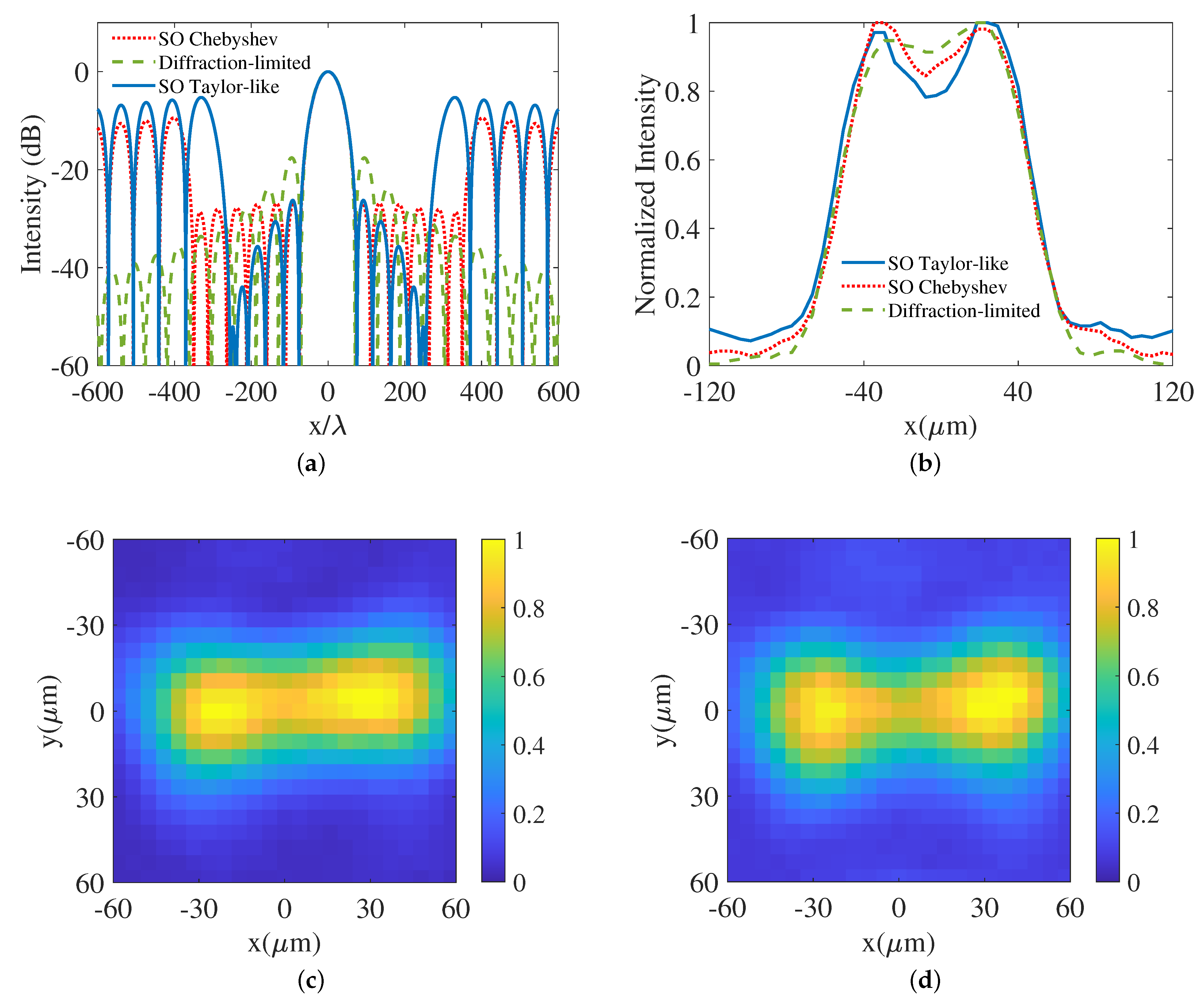
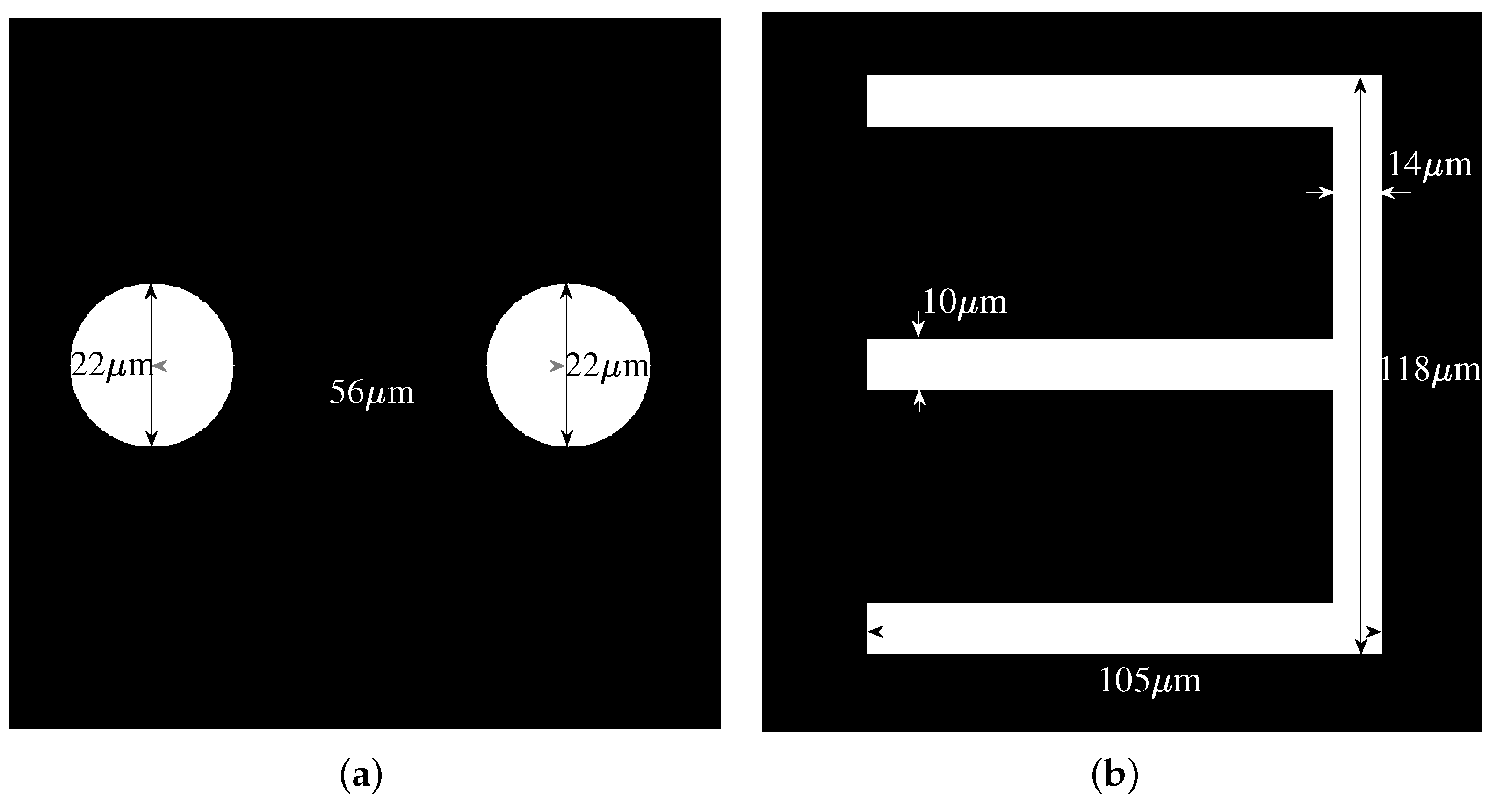
To showcase the resolution improvement owing to the tapered sidelobes, we design both Chebyshev and Taylor-like point-spread functions with super-oscillatory sidelobes, by which we image two objects as shown in Figure 16a. The imaging results for the object of two apertures are given in Figure 14. In Figure 14a, the FWHM, first sidelobe level and radius of the ROI for the Taylor-like super-oscillatory point-spread function is 37.6 $\mathsf{\mu }$m, −26.2 dB and 161.5 $\mathsf{\mu }$m. As shown in Figure 14a, the Taylor-like point-spread function has a tapered sidelobe structure that results in a lower dip in Figure 14b. 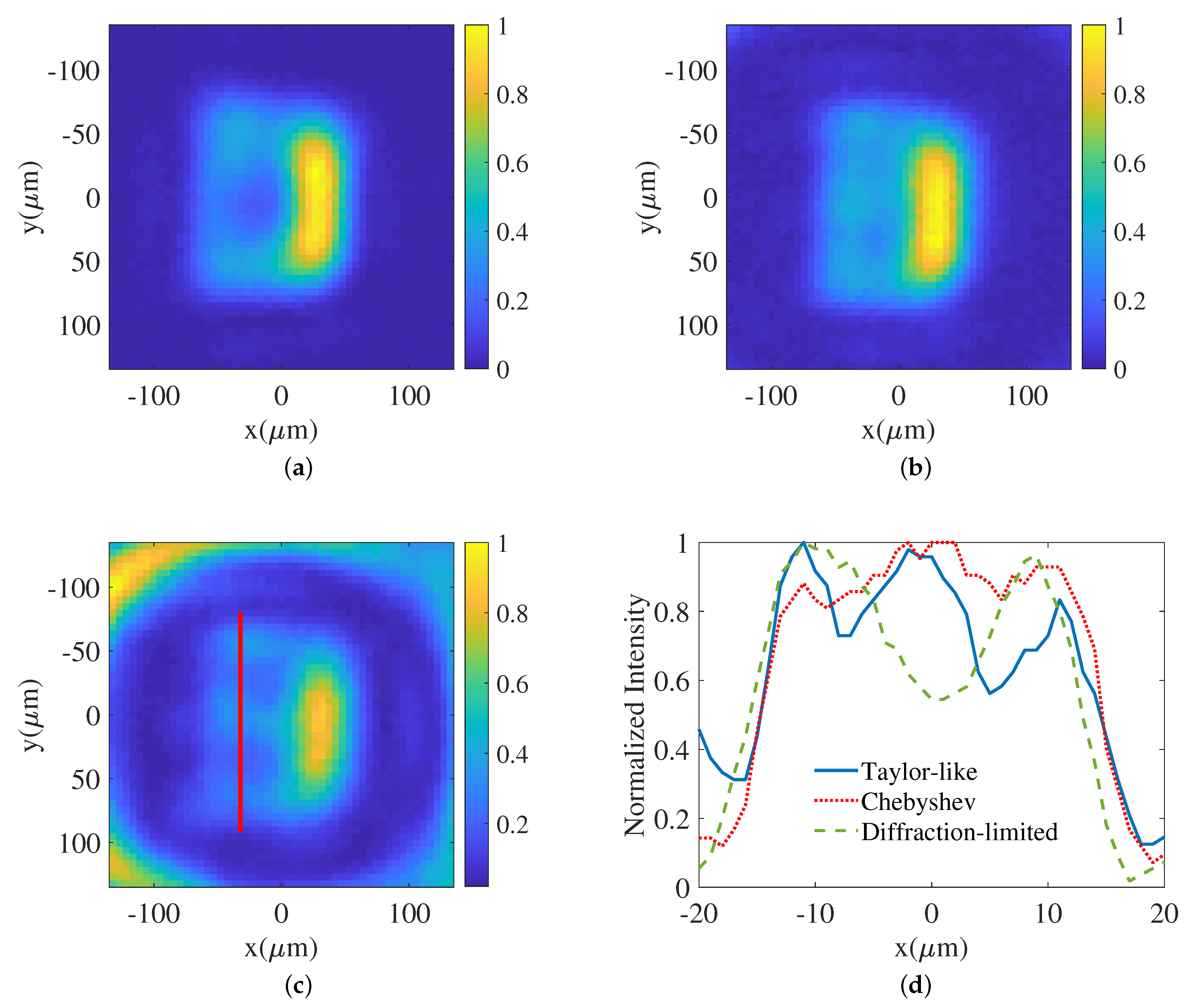This improved resolution can also be observed by the comparison of the images in Figure 14c,d. To further demonstrate the super-resolution ability of the Taylor-like super-oscillatory point-spread function, we manage to image a transmissive mask with the letter E (see Figure 16b) by Chebyshev and Taylor-like point-spread functions with super-oscillatory sidelobes. As shown in Figure 15a–c, the image captured with the Taylor-like point-spread function has the best resolution that is also illustrated in Figure 15d by drawing the intensity distribution of the three branches of the letter E compared to the corresponding Chebyshev and diffraction-limited ones. The resolution improvement in imaging the objects of the two apertures and the mask with the letter E results from reduced sidelobe interference by the tapered sidelobes since the only difference regarding resolving objects between the Chebyshev and Taylor-like point-spread functions in Figure 14a is the sidelobe structure. The reduced sidelobe interference can be explained by the following statement. The imaging process can be expressed by

$$I=obj\otimes psf$$

(33)

where I is the complex field on the image plane, $obj$ is the object to be imaged, $psf$ is the coherent point-spread function, and ‘⊗’ denotes the convolution. When the convolution is conducted, the value of one element in the image I is decided by

$$I(m,n)=\int obj(x,y)·psf(m-x,n-y)dxdy$$

(34)

from which, it is found that $I(m,n)=obj(m,n)$ if $psf$ is a Dirac $\delta$ function that has no sidelobes. Otherwise, $I(m,n)=obj(m,n)+\mathsf{\Delta }I$ where the main beam of the $psf$ is still assumed to be infinitely narrow, and $\mathsf{\Delta }I$ denotes the sidelobe inteference that is the sum of multiplications of the sidelobes and other parts of $obj$ except $obj(m,n)$. In the incoherent imaging system, lower sidelobes give less interference when imaging the in-phase objects. The reason is that the incoherent $psf$ is non-negative [33]. In the coherent system, it becomes hard to quantitatively analyze $\mathsf{\Delta }I$ because the multiplications of the sidelobes and parts of $obj$ might be positive or negative. However, this goal becomes clear in the ideal case where $\mathsf{\Delta }I=0$. Reducing the sidelobe level can lower $\mathsf{\Delta }I$. Thus, we can reasonably expect better resolution by the Taylor-like point-spread functions with tapered sidelobes, compared to the Chebyshev one, because the former one is a better approximation to an ideal Dirac $\delta$ function in terms of the sidelobe levels.

Furthermore, it is observed that the imaging intensity of the letter E in the ROI is low. This is mainly caused by the fact that a large portion of the illumination energy is distributed to the sidebands (see Figure 10 for the definition). Two possible solutions to resolve this issue are increasing the illumination power and using a high-dynamic-range imaging technique [34]. When Figure 15b is compared with Figure 15c, there seems to be more sidelobe interference in the Taylor-like case. Actually, this phenomenon is as a result of the sidebands. As is shown in Figure 14a, the super-oscillatory Chebyshev point-spread function has a larger ROI than the Taylor-like one. The radius of the ROI for the Chebyshev one is 221.3 $\mathsf{\mu }$m, whereas this is only 161.5 $\mathsf{\mu }$m for the Taylor-like one. This implies that the sidebands in the Taylor-like one occupy more energy from the illuminated power. Thus, less energy would be used to form the image in the ROI. The resultant phenomenon is that the signal-to-noise ratio in the Taylor-like case is lower than in the Chebyshev case.

There are several reported works on super-oscillatory imaging and focusing based on the particle swarm optimization [5,35], the genetic algorithm [36], and the linear programming method [37]. These algorithms are all based on specified objective functions and multiple constraints. Since these algorithms search for the optimal solution in the search-space, they are iterative methods. In contrast, in our synthesis method, as long as the number of total zeros, the number of zeros inside the visible region, the size of the ROI, and the first sidelobe level are specified, the super-oscillatory pattern can be produced directly without any numerical iterations. The sidelobes in Refs. [35,36] are not tapered, which indicates that there is no control over the sidelobe structure to reduce the interference arising from the sidelobes. In this present work, the sidelobes are tapered in a user specified manner. It is pointed out [36,37] that there is a trade-off between the FWHM of the main beam (hotspot), the sidelobe level within the ROI, and the size of the ROI. It is worth noting that prominent sidebands (that surround the sidelobes and the main beam) are non-existent in the super-oscillatory point-soread functions in Refs. [35,36], which implies that raising the sidelobe level to reduce the FWHM of the main beam is basically the approach utilized in these works. Thus, the sidelobe interference would finally become unbearable when squeezing the main beam further. On the other hand, the appearance of sidebands in Refs. [11,37] could help relieve this exasperation because the sidelobes inside the ROI can be reduced to a low level and an arbitrary sub-diffraction main beam is still attainable. Furthermore, the size of the ROI surrounded by the sidebands can be customized by the synthesis method proposed in this paper, which ensures the availability of the non-scanning mode in our super-oscillatory imaging system compared to the scanning mode used in Ref. [5]. It only takes several milliseconds for us to capture the complete image. Thus, the size of the ROI and the sidelobes inside the ROI can be balanced simultaneously. When imaging extended objects, the ROI would undoubtedly put a limitation on the size of the objects. The possible solution in our super-oscillatory imaging system is to enlarge the super-oscillatory field of view whose radius is decided by $2\pi /\mathsf{\Delta }k$ where $\mathsf{\Delta }k$ is the sampling interval of the Fourier components on the Fourier plane. This implementation is simply increasing the number of Fourier components to be modulated, which is limited by the resolution of the SLM. If the size of the object is beyond the ROI limit allowed by the super-oscillatory imaging system, the possible way out is by utilizing a pinhole, whose size should be smaller than the ROI limit, in front of the object and scanning the object.

6. Conclusions

This work introduces a method to design two types of super-oscillatory Taylor-like point-spread functions by means of Schelkunoff’s super-directive antenna theory. Simulation results exploring super-directive patterns, zeros distribution and excitation weights are outlined. The one-parameter Taylor-like super-directive pattern offers a faster tapering rate than the $\overline{n}$ type one. The parameters controlling the main beamwidth and sidelobe level structure are explored. To make the synthesis practical in terms of the large amount of stored energy in the near-field for super-directive antennas, we place extra zeros into the invisible region, which can efficiently lower the maximum excitation weighting ratio. This technique, when applied to synthesizing the super-oscillatory point-spread functions, can reduce the intensity of the sideband that is an inherent drawback of super-oscillations. In the experimental section, we first conduct an experiment for obtaining the point-spread function of Taylor-like super-oscillations, which has tapered sidelobes and narrower main beamwidth compared to the diffraction-limited point-spread funcion. This is done by means of advanced programmable gratings formed on an SLM. We then verify the superiority of its tapered sidelobes over the equal sidelobes of Chebyshev patterns by imaging two objects using a 4F imaging system. It is shown that tapered sidelobes can reduce the interference from the sidelobes and therefore improve the resolution. In detail, the imaging results of a two-aperture object show a lower dip with the Taylor-like super-oscillatory point-spread function. In the experiment of imaging a mask with the letter E, the result with the Taylor-like pattern has the best resolution in resolving its three branches compared to the corresponding Chebyshev and diffraction-limited patterns. It can be envisioned that this Taylor-like super-oscillatory point-spread functions would help mitigate the unwanted effects caused by sidelobes in super-oscillatory imaging, such as artifacts and imaging ambiguity.