Squeezed Coherent States in Double Optical Resonance


1
Department of Physics, University of Crete, P.O. Box 2208, GR-71003 Heraklion, Greece
2
Institute of Electronic Structure and Laser, FORTH, P.O. Box 1527, GR-71110 Heraklion, Greece
*
Author to whom correspondence should be addressed.
Photonics 2021, 8(3), 72; https://0-doi-org.brum.beds.ac.uk/10.3390/photonics8030072
Submission received: 4 February 2021
/
Revised: 24 February 2021
/
Accepted: 26 February 2021
/
Published: 5 March 2021
(This article belongs to the Special Issue Quantum Optics in Strong Laser Fields)
Abstract
:In this work, we consider a “-type” three-level system where the first transition is driven by a radiation field initially prepared in a squeezed coherent state, while the second one by a weak probe field. If the squeezed field is sufficiently strong to cause Stark splitting of the states it connects, such a splitting can be monitored through the population of the probe state, a scheme also known as “double optical resonance”. Our results deviate from the well-studied case of coherent driving indicating that the splitting profile shows great sensitivity to the value of the squeezing parameter, as well as its phase difference from the complex displacement parameter. The theory is cast in terms of the resolvent operator where both the atom and the radiation field are treated quantum mechanically, while the effects of squeezing are obtained by appropriate averaging over the photon number distribution of the squeezed coherent state.
1. Introduction
One of the most intriguing accomplishments of quantum optics over the last 35 years is the ability to generate quantum states of light that do not have any classical analog and tailor their statistical properties. Among these states of non-classical radiation, there is a class of states that have received considerable attention both from a theoretical, as well as from an experimental viewpoint due to their numerous applications [1] in modern quantum technologies, i.e., the “squeezed” states of radiation [2]. A quantum state is referred to as “squeezed” if the variance of one of the quadrature amplitudes of the state is modified in such a way that it becomes smaller than the respective variance of a vacuum or a coherent state. Such states are referred in the bibliography under the terms “Squeezed Vacuum State” (SQVS) and “Squeezed Coherent State” (SQCS), respectively. Due to Heisenberg’s uncertainty principle, squeezing always results in the increase of the conjugated quadrature variance above the variance of a vacuum, in the case of the former, and the variance of a coherent state, in the case of the latter [3].
The first experimental observation of squeezed light was reported back in 1985 in the pioneering work of Slusher et al. [4], who achieved four-wave-mixing in an atomic vapor of sodium atoms. Since then, significant advances in the generation and detection of squeezed light [5] gave the green light for the implementation of squeezing as a resource in a series of different applications in basic research and technology. Among these applications, the ones that stand out are related to the reduction of quantum noise in optical communications [6], the detection of sub-shot-noise phase shifts [7,8], the ability to achieve maximum sensitivity in interferometry at lower laser powers [9], which was implemented in the detection scheme of gravitational waves [10], the storage of quantum memory [11,12], necessary for quantum information tasks, and most recently, the ability of quantum-enhanced microscopy and effective bio-imaging without the danger of damaging the cell sample [13,14].
The underlying physical mechanism behind the last application is thoroughly intriguing since it is based on the effective yield enhancement that one can achieve by inducing non-linear processes with squeezed radiation. As has been known since the 1960s [15,16], any non-linear light-matter interaction depends on the quantum statistical properties of the radiation that are embodied in its correlation functions. This realization naturally led to a series of studies [17,18,19,20,21,22,23,24,25,26,27,28,29,30] on non-linear phenomena induced by fields that may exhibit photon bunching or superbunching properties, resulting in values of the intensity correlation functions higher than those of a coherent state. The simplest example illustrating this dependence is the transition from a bound state to a continuum via the absorption of N photons, i.e., N-photon ionization. The derivation of the transition probability per unit time for N-photon ionization when all real bound atomic intermediate states are assumed sufficiently far from resonance [31,32,33,34] indicates that the rate of the process is proportional to an effective N-photon matrix element multiplied by the Nth-order intensity correlation function [15,16]. In view of the dependence of the correlation functions on the stochastic properties of the radiation, the rate of such a process can be affected dramatically by the intensity fluctuations of the source [35]. As a prototype example, one can take an 11-photon ionization process induced by thermal radiation whose Nth order intensity correlation function is given by , where I is the average intensity, i.e., times larger than the respective correlation function of the coherent field. For , the factor arising from the strong intensity fluctuations of the chaotic field gives us an enormous enhancement of around seven orders of magnitude, which in fact has been observed experimentally in the past for a process of such a high order [36,37]. The situation becomes even more interesting if one considers squeezed radiation, which under certain values of the parameters may exhibit superbunching properties resulting in correlation functions even larger than those of the chaotic field [38]. As an example, the Nth order correlation function of a bright (high intensity) SQVS is times larger than the respective correlation function of the coherent field [39], an enhancement factor even larger than the of the chaotic field. This enhancement factor has been measured experimentally in a recent work by Spasibko et al. [40] by generating optical harmonics of the order of 2–4 from a bright SQVS.
The pronounced interplay between the non-linear character of an atomic transition [41] and the photon correlation effects of the radiation that induces it has also been investigated in the context of the dynamics of an atomic transition between two bound states that are connected via a strong field with various quantum photon statistics. In this scenario, the dynamics can be monitored either through the calculation of the spontaneous emission spectrum of the upper state (fluorescence) or through the calculation of the population of a third state weakly connected to one of the two bound states, serving as a probe. The second scheme is often found in the bibliography under the term “Double Optical Resonance” (DOR) [42,43]. If the driving field connecting the two bound states is sufficiently strong, then each of the two states is split into doublets, whose energy separation depends on the coupling strength with the field. This effect is widely known as Stark or Autler–Townes splitting [44]. The case of strong driving by a chaotic field of arbitrary bandwidth has been investigated in great detail [45,46,47,48] and predicts a variety of interesting discrepancies from the well-studied case of coherent driving, which to the best of our knowledge still remain to be explored experimentally. The problems of resonance fluorescence into a squeezed vacuum reservoir [49,50,51,52,53,54,55,56,57], as well as the weak-field absorption of a two-level atom by various quantum states of radiation in the narrow bandwidth limit [58] have also been investigated in depth.
In a recent work [59], we studied the single- and two-photon Autler–Townes splitting profile in realistic atomic transitions driven by bunched and superbunched radiation and obtained a counterintuitive behavior resulting from the complex interplay between the form of the photon probability distributions of the squeezed vacuum and chaotic fields and the compounded non-linearity of the system, arising both from the strong driving and the order of the process. Our results indicated that much has to be still discovered concerning the strong interaction between atoms and non-classical radiation. The main hindrance in the experimental investigation of such systems so far has been the difficulty of producing stable, high intensity squeezed sources with controllable stochastic properties in the lab. However, in view of recent works [60] providing novel methods to overcome experimental difficulties associated with the generation of squeezed coherent radiation, the study of the strong driving of a bound-bound transition by a radiation field initially prepared in an SQCS is timely. Since squeezed light is not amenable to simulation in terms of classical stochastic processes, we adopt a fully quantum mechanical treatment in terms of the resolvent operator, involving averaging over the photon number distribution of the SQCS, a method valid in the “zero bandwidth” limit, i.e., in the limit where the bandwidth of the source is sufficiently smaller than the natural decay of the excited state.
2. Materials and Methods
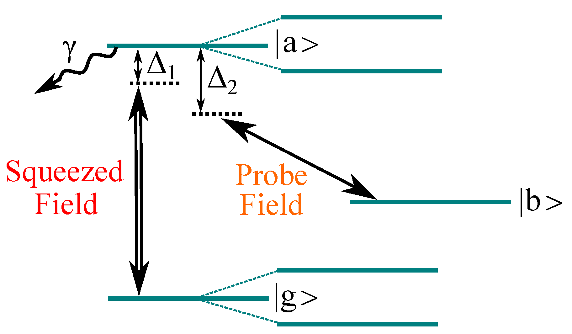
We begin by considering an atom initially resting in its ground state in the presence of a quantized radiation field in a two-mode Fock state with n photons in the first mode with frequency and m photons in the second mode with frequency . The atom can absorb one photon from the first mode and move to the excited state , while the latter is coupled to another excited state via the emission of one of the m photons. The Hamiltonian of the system consists of three parts, namely: the atomic Hamiltonian , the Hamiltonian of the radiation field , and the interaction Hamiltonian under the rotating wave approximation, , where , , and are the energies of the atomic states , , and , respectively, and represent the coupling strengths between those states in units of frequency, while and are photon annihilation and creation operators, respectively. The atomic operators and are the raising and lowering operators, respectively, given by the relations , , , and .
The eigenstates of the unperturbed Hamiltonian of the compound system “atom + radiation” are , , and , with energies , , and , respectively. The detunings from resonance of the two transitions are defined as and .
To account for the spontaneous decay of the excited state , we make the substitution , in view of which, our system now becomes open. Note that this method introduces a decay rate without accounting for the repopulation of the ground state. It is however a good approximation as long as the first transition is sufficiently strong so that the Rabi frequency of the first transition is sufficiently larger than the decay rate . In such a case, the interaction between the uncoupled states of the compound system and causes a splitting into doublets energetically separated by (Stark splitting). Such a splitting can be monitored through the calculation of the probe state population (state ) as a function of . Our ultimate goal is the study of the splitting profile in the case where the transition is driven by a strong field prepared in a squeezed coherent state. The switch over from the initial Fock state to a squeezed coherent state can be realized through appropriate averaging of the probe state population over the photon statistics distribution of the squeezed coherent field, as will be described in detail below. A schematic presentation of the system we study is depicted in Figure 1.
Our problem is formulated in terms of the resolvent operator, which is the Laplace transform of the time evolution operator . Taking the Laplace transform with s being the usual Laplace variable and making the change of variables s = −iz, we obtain the relation , where is the resolvent operator [29,61,62]. Using the relation , it is straightforward to show that obeys the equation , where is the unperturbed resolvent operator. In view of this equation, the matrix elements of the resolvent operator in the compound system basis satisfy the equations:
Solving for , one obtains:
The matrix elements of the time evolution operator in the compound system basis, i.e., , , are related to the respective matrix elements of the resolvent operator through the inverse transform [29,61,62]:
where , with . In order to calculate the integral of Equation (5), one should first calculate the roots of the third order polynomial appearing in the denominator of Equation (4). If we denote these three roots by , , and , the resulting expression is:
The population of the probe state at times is given by:
The population of depends non-linearly on the photon numbers n and m through the expressions of the compound system energies , , and , as well as the matrix elements and that reflect the Rabi frequencies of the and transitions, respectively, via the relations and .
We focus on the dependence of on n and t, by adopting the notation . The dependence on m is not of particular importance as long as the probe field coupling strength is chosen to be sufficiently smaller than all the other rates that appear in the problem at hand. To capture the case where the field driving the is initially prepared in a state other than Fock, one can average the desired quantity (probe state population in our problem) over the corresponding photon number distribution of the initial field state. This is a standard method in quantum optics [63]. However, one should note that it is strictly valid in the “zero bandwidth” approximation, i.e., in the limit where the field bandwidth is much smaller than the natural decay . We are particularly interested in the case where the field driving the first transition is initially prepared in an SQCS.
An SQCS is defined as the state resulting upon acting on the vacuum state with the squeezing operator followed by the displacement operator , i.e.:
The squeezing and displacement operators are given by the relations and , respectively, where is the complex squeezing parameter and is the complex displacement parameter. The photon number distribution of an SQCS is given by [64]:
where is the -order Hermite polynomial. By substituting in Equation (9) and adopting the definition , one finally gets:
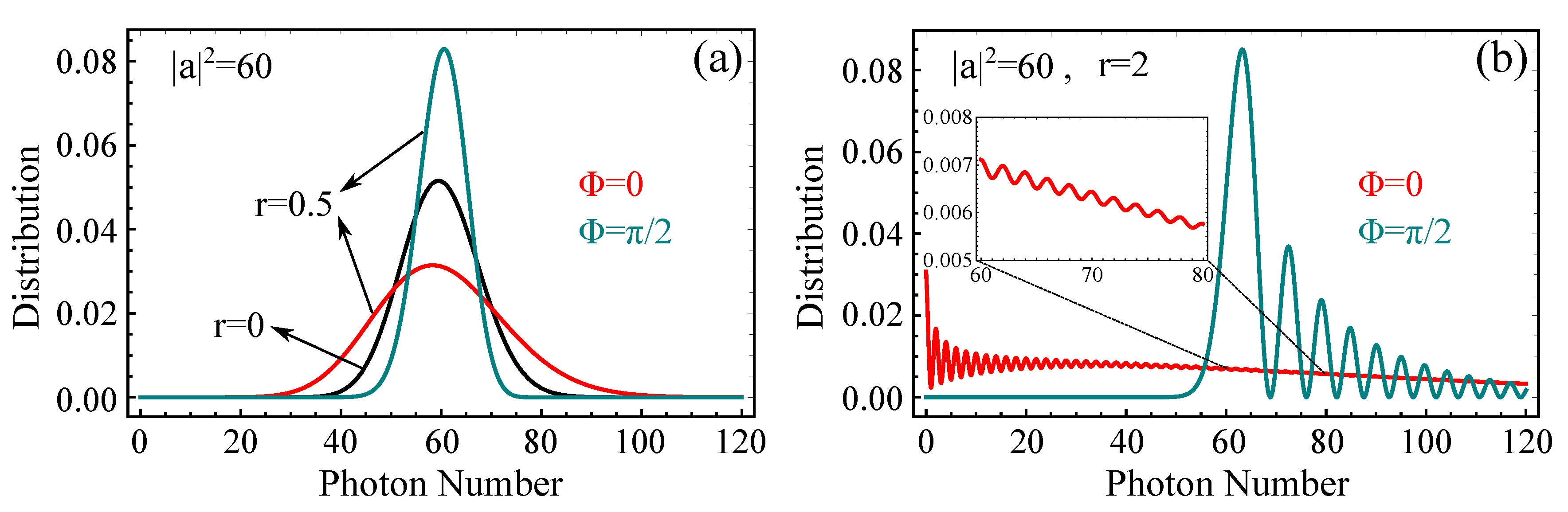
In Figure 2a, we plot the photon number distribution of an SQCS with a squeezing parameter and compare it to the distribution of a coherent field (). As becomes evident, depending on the phase difference , the distribution deviates from its Poissonian form, by exhibiting super-Poissonian (red line) or sub-Poissonian statistics (teal line). The situation becomes even more interesting for larger values of r. In Figure 2b, we plot the photon number distribution of an SQCS with a squeezing parameter for two values of and observe an obvious non-classical behavior with vivid oscillations in both cases. These oscillation were interpreted in the past by Schleich and Wheeler [65,66] as resulting from the interference of error contours in phase space. In the case (red line), the distribution is peaked at , and the oscillations are much faster compared to the case (teal line), where the distribution is peaked at a slightly higher photon number than the peak of the Poissonian distribution and the oscillations appear only for photon numbers larger than the position of the peak. It should be noted that the photon number distributions of Figure 2 acquire discrete values for each value of the integer n, but are depicted as continuous since the photon number scale over which they are plotted is large. To avoid any misconception, there is another form of Equation (10) often found in the bibliography where the distribution is essentially the same, but it exhibits sub-Poissonian statistics for and super-Poissonian statistics for . This is a reflection of whether the SQCS is defined as or , which are not equal since the operators and do not commute. In any case, one can go from one definition to the other through the relation:
Returning back to our problem, we average the population of the probe state over the photon number distribution of Equation (10), according to:
In what follows, we will be concerned about the behavior of as a function of for different parameters of the SQCS, or put otherwise, the effects of various schemes of squeezing on the resulting Stark splitting profile imprinted on the population of the probe state.
3. Results and Discussion
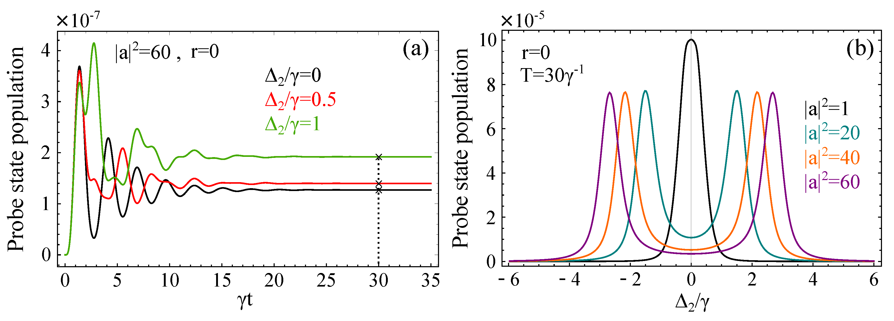
Among other parameters, Equation (12) depends also on time. Therefore, in order to study the behavior of the probe state population as a function of , one should first make a choice of the interaction time during which the driven system is exposed to the radiation. In Figure 3a, we plot as a function of time for various detunings and . Under this choice of parameters, we notice that the population of the probe state reaches its steady-state value at about . Numerical investigations of the behavior of as a function of time for different combinations of the parameters , , r, and revealed that the choice of always guarantees that the system is well within its steady-state regime. Therefore, we adopt this choice of time for the calculations throughout the paper. In Figure 3b, we plot as a function of for various and parameters corresponding to a coherent state. Note that, as expected, for , the distribution does not depend on the choice of . We confirm that as increases and the mean Rabi frequency becomes larger than the spontaneous decay rate , the single peak structure (black line) splits into two peaks forming the well-known Autler–Townes doublet structure [44]. The distance between the two peaks is equal to the mean Rabi frequency , which is proportional to the square root of the mean photon number of the coherent state . As long as is smaller than , the increase of will result in power broadening of the profile [67] until it splits into the doublet.
Before continuing to the case of strong driving by an SQCS, we should note that the exact choice of the Rabi frequency of the probe transition is not of direct relevance to our problem, as long as it is sufficiently weaker than all of the other rates that appear in the derivation. If this condition is satisfied, then the only effect of changing the Rabi frequency of the probe will be a linear change in the total population of the probe state (y-axis), but not in the ratio between individual peaks or widths. Since our aim is the study of the form of the splitting profile, the exact values of the probe state population are of no importance. For the same reason, we are not concerned about the possible natural decay of the probe state to some other unobserved state.
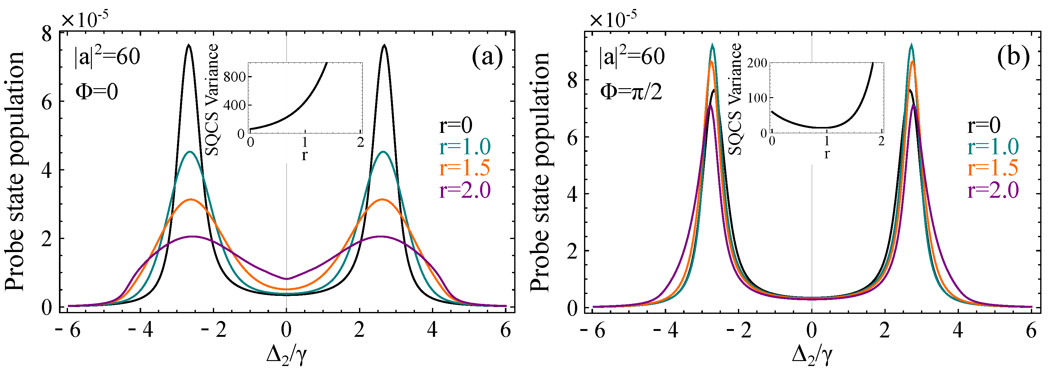
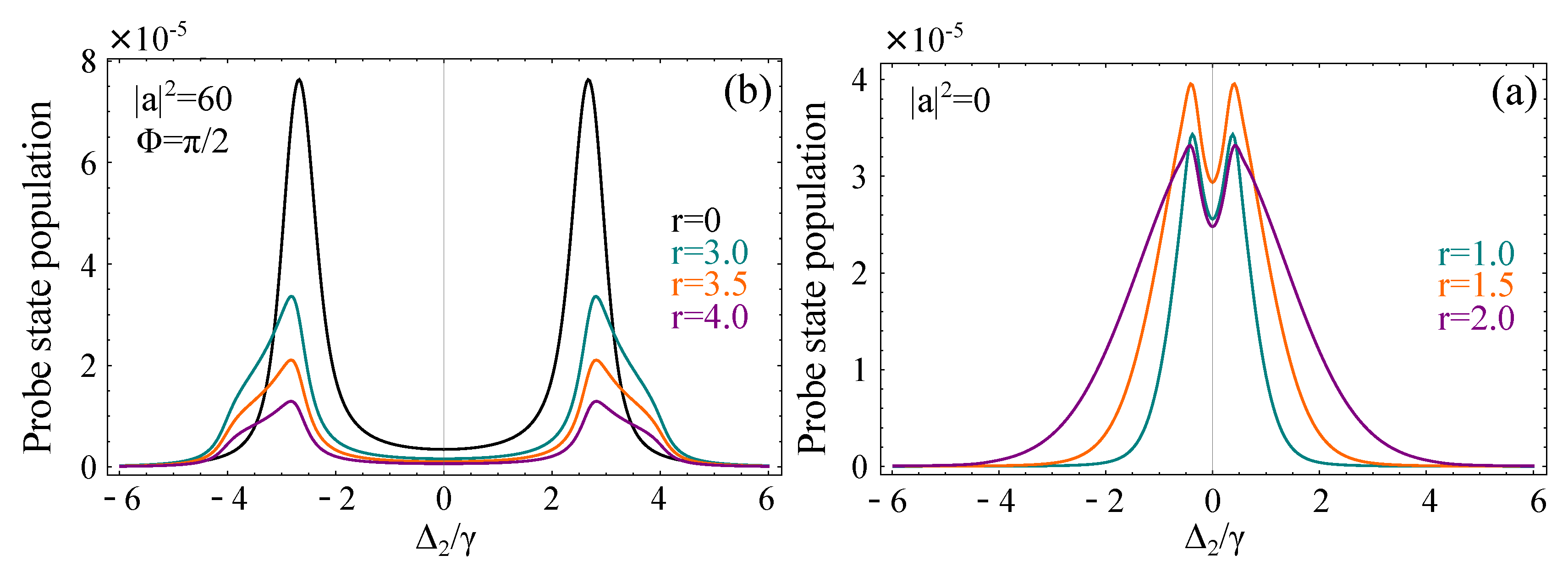
In Figure 4a, we plot the population of the probe state as a function of for various degrees of squeezing and . The splitting profile shows great sensitivity to the value of the squeezing parameter r, becoming significantly broader as the latter increases. The physics behind this broadening of the profile is related to the strong amplitude fluctuations of the field that are translated into fluctuations in the value of the Rabi frequency of the transition that cause partial smearing of the doublet structure after taking the average over the SQCS distribution. However, as seen in Figure 4b, under the same choice of parameters, but with , the profile only slightly deviates from the profile exhibited under coherent state driving (). An effective way of interpreting this sensitivity on the phase difference is through the form of the SQCS photon number variance. In particular, the photon number variance of the SQCS is given by the relation [68]:
For , Equation (13) reduces to . In this case, it is straightforward to show that the increase of the squeezing parameter will always lead to the increase of the variance of the SQCS (inset of Figure 4a) and therefore to the broadening of the total profile after averaging over the SQCS distribution. However, the picture is drastically different if , where Equation (13) takes the form . It is easy to check that in this case, the variance is not increasing monotonically as a function of r, but it acquires a minimum value at a position that depends on the choice of . In the considered case , the minimum is positioned at . The variance remains smaller than its value at (corresponds to a coherent state) up to the position and becomes larger than that thereafter (inset of Figure 4b). Furthermore, the value of the variance in the vicinity of the minimum is not much smaller than its value. This behavior explains why for the squeezing parameters considered in Figure 4b, the SQCS splitting profile does not exhibit significant deviations from the corresponding coherent profile. It also explains why the peaks of the teal and orange lines corresponding to the values and , respectively, appear larger than the peaks of the black line (coherent field), due to the sub-Poissonian form of the SQCS photon number distribution.
As r increases, for , the peaks of the splitting profile appear at slightly smaller detunings than the coherent splitting, contrary to the case where the peaks tend towards higher detunings. This can be attributed to the behavior of the mode of the SQCS distribution (most probable value) as a function of r in each case. In particular, for , the mode of the distribution tends towards the zero photon number, while for , it is positioned at photon numbers slightly higher than , depending on the value of r. This tendency is also evident in Figure 2. We should note that the peaks of the resulting profile are not separated by the Rabi frequency corresponding to the mode of the photon number distribution, nor the Rabi frequency corresponding to its mean photon number, given by the relation , for every . As argued in previous work, the exact shape of the resulting profile stems from a complex interplay between the properties of the probe state population function associated with the order of the process and the structure of the photon probability distributions of the driving field [59]. The behavior of the mode as a function of r and different values of can however give us good evidence for the expected behavior of the position of the peaks.
This tendency of the peaks towards slightly higher (absolute) detunings for as r is increased, i.e., the increasing in the frequency distance between the two peaks, becomes even more evident by inspecting Figure 5a. In this figure, we examine the resulting profile for very large values of the squeezing parameter corresponding to well beyond the state-of-the-art squeezing. At this point, we should mention that squeezing is most usually measured in the bibliography in terms of the squeezing factor in dB units. The connection between the squeezing factor R and the squeezing parameter r used in our work is given by the relation:
Therefore, the very high squeezing factor of 20dB reported back in 2016 [69] corresponds approximately to a squeezing parameter . As becomes evident in Figure 5a, under extreme squeezing, the resulting profile is distorted in a rather unusual way. The peaks of the profile are positioned at even higher detunings from those of Figure 4b, and the total profile is broadened mainly towards one direction. This effect can be interpreted through the particular form of the SQCS photon number distribution for . As seen in Figure 2b, the distribution exhibits a large peak at a photon number slightly higher than , followed by an oscillatory behavior for larger photon numbers. As r increases, the distribution maintains its form qualitatively, but the probability of the mode (most probable value) of the distribution tends towards larger values, while the ratio of the probabilities between subsequent peaks of the distribution is decreased. This indicates that as r is increased, the weight of the distribution is transferred from its mode towards the peaks of higher photon numbers, leading also to the increase of the variance of the distribution. Therefore, the splitting profile after averaging over the SQCS distribution exhibits smaller peaks, but it is more broadened towards higher (absolute) detunings.
Another interesting scenario occurs for , but a non-zero squeezing parameter. This choice of parameters corresponds to what is widely known as a squeezed vacuum state (SQVS). The SQVS is defined as , and its photon number distribution is given by:
where is the mean photon number of the distribution. As seen from Equation (15), the SQVS distribution exhibits oscillatory behavior with zero values for odd photon numbers. The mode of the distribution is sharply peaked at , and its variance is given by the relation . In Figure 5b, we plot the population of the probe state when the strong field is initially prepared in an SQVS. In agreement with previous work [59], we notice that the positions of the peaks are rather insensitive to the increasing of the squeezing parameter (translated to intensity in [59]), while the widths of the peaks are significantly increased, as one would expect by inspecting the SQVS variance for increasing r. From a physical viewpoint, this sharp increase of the width is due to the superbunching effect inherent in squeezed vacuum sources, translated to strong intensity fluctuations that smear out the profile. Note that the exact shape of the profile also depends on the choice of the coupling strength , which is however chosen to be the same through all of our calculations (), providing us the ability for straightforward comparison between the profiles of different figures.
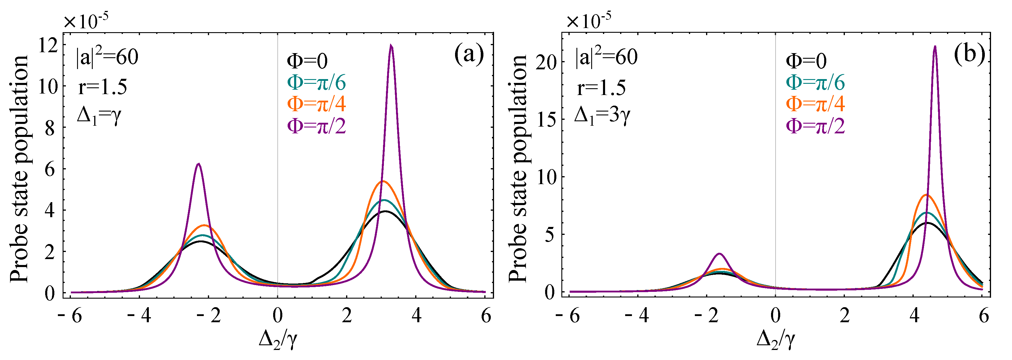
Lastly, in Figure 6a,b, we consider the case where the squeezed field is detuned from resonance with the transition. Similar to the case of coherent driving, the profile exhibits an asymmetry with the larger peak appearing at positive detunings for positive , and vice versa. This asymmetry can be interpreted in terms of the dressed states of the strong field transition [42]. The resulting doublets are expressed as linear combinations of the ground and the first excited state of the atom, with equal weights in the case of exact resonance ( = 0). However, as is increased, one can show that the upper dressed state of the doublet contains more of the state and less of the ground state, while the opposite is true for the lower dressed state. In this case, the probe state is connected through a larger dipole moment to the upper state of the doublet than the lower, resulting in an asymmetry in the splitting profile. The asymmetry is examined for and various values of the phase difference . As is increased, the width of the two peaks is decreased, and the peaks move towards slightly higher detunings (their frequency distance is increased). The width of each peak also depends on . Increasing results in the decrease of the width of the large peak and the increase of the width of the smaller one. Finally, we report that the asymmetry ratio (peak-to-peak) does not remain constant, but it increases with the increase of .
4. Concluding Remarks
In this work, we have examined the Autler–Townes splitting profile resulting from the strong driving of two bound atomic states by an SQCS. The splitting was probed through a third state assumed to be weakly coupled to the upper bound state in a three-level “-type” system. Since squeezed radiation is not amenable to modeling in terms of classical stochastic processes, we adopted a fully quantum mechanical treatment in terms of the resolvent operator and averaged the population of the probe state over the photon number distribution of the SQCS in the zero-bandwidth limit, i.e., in the limit where the bandwidth of the squeezed field is sufficiently smaller than the natural decay of the excited state. Our results indicate that the resulting splitting profile is greatly affected by the parameters of the SQCS, i.e., the squeezing parameter r and its phase difference from the complex displacement parameter. In particular, we showed that for , the profile becomes significantly broader with the increase of r, while under the same values of parameters, but with , increasing r up to two results in a profile resembling the one acquired with coherent driving. This degree of squeezing is well within today’s squeezing capabilities, while the intensities necessary for the observation of single-photon Stark splitting in atomic systems are of the order of 1 W/cm [59]. The case of extreme squeezing was also investigated, revealing unusual distortions of the splitting profile, as well as the cases of SQVS driving and off-resonant strong driving resulting in an asymmetric profile. To the best of our knowledge, the investigation of the strong driving of a bound-bound atomic transition by an SQCS remains still an open and interesting experimental problem. At the same time, recent progress in quantum engineering using ion traps opens up the possibility to efficiently prepare squeezed states of ionic motion that do not posses any classical analog [70,71,72]. Although such systems are not directly analogous to our system of study, they should be highlighted before closing this work, due to their numerous applications in spectroscopy, in quantum metrology, and in quantum information technology [73].
Author Contributions
Both authors contributed in the conceptualization, methodology and preparation of the manuscript. All authors have read and agreed to the published version of the manuscript.
Funding
This research was funded by the IESL FORTH Research and Development Program E00710.
Acknowledgments
G.M. would like to acknowledge the Institute of Electronic Structure and Laser (IESL), FORTH, for financially supporting this research by its Research and Development Program E00710.
Conflicts of Interest
The authors declare no conflict of interest.
Abbreviations
The following abbreviations are used in this manuscript:
| SQVS | Squeezed Vacuum State |
| SQCS | Squeezed Coherent State |
| DOR | Double Optical Resonance |
References
- Walls, D.F. Squeezed states of light. Nature 1983, 306, 141–146. [Google Scholar] [CrossRef]
- Breitenbach, G.; Schiller, S.; Mlynek, J. Measurement of the quantum states of squeezed light. Nature 1997, 387, 471–475. [Google Scholar] [CrossRef]
- Loudon, R.; Knight, P. Squeezed Light. J. Mod. Opt. 1987, 34, 709–759. [Google Scholar] [CrossRef]
- Slusher, R.; Hollberg, L.; Yurke, B.; Mertz, J.; Valley, J. Observation of squeezed states generated by four-wave mixing in an optical cavity. Phys. Rev. Lett. 1985, 55, 2409. [Google Scholar] [CrossRef] [PubMed]
- Andersen, U.L.; Gehring, T.; Marquardt, C.; Leuchs, G. 30 years of squeezed light generation. Phys. Scripta 2016, 91, 053001. [Google Scholar] [CrossRef]
- Yuen, H.P. Two-photon coherent states of the radiation field. Phys. Rev. A 1976, 13, 2226. [Google Scholar] [CrossRef] [Green Version]
- Xiao, M.; Wu, L.A.; Kimble, H.J. Precision measurement beyond the shot-noise limit. Phys. Rev. Lett. 1987, 59, 278. [Google Scholar] [CrossRef] [PubMed] [Green Version]
- Grangier, P.; Slusher, R.E.; Yurke, B.; La Porta, A. Squeezed-light–enhanced polarization interferometer. Phys. Rev. Lett. 1987, 59, 2153. [Google Scholar] [CrossRef]
- Caves, C.M. Quantum-mechanical noise in an interferometer. Phys. Rev. D 2020, 23, 1693. [Google Scholar] [CrossRef] See also: Chia, A.; Hajdušek, M.; Nair, R.; Fazio, R.; Kwek, L.C.; Vedral, V. Phase-Preserving Linear Amplifiers Not Simulable by the Parametric Amplifier. Phys. Rev. Lett. 2020, 125, 163603. [Google Scholar] [CrossRef]
- Abbott, B.P.; Abbott, R.; Abbott, T.D.; Abernathy, M.R.; Acernese, F.; Ackley, K.; Adams, C.; Adams, T.; Addesso, P.; Adhikari, R.X.; et al. Observation of Gravitational Waves from a Binary Black Hole Merger. Phys. Rev. Lett. 2016, 116, 061102. [Google Scholar] [CrossRef] [PubMed]
- Kozhekin, A.E.; Mølmer, K.; Polzik, E. Quantum memory for light. Phys. Rev. A 2000, 62, 033809. [Google Scholar] [CrossRef] [Green Version]
- Appel, J.; Figueroa, E.; Korystov, D.; Lobino, M.; Lvovsky, A.I. Quantum Memory for Squeezed Light. Phys. Rev. Lett. 2008, 100, 093602. [Google Scholar] [CrossRef] [PubMed] [Green Version]
- Li, T.; Li, F.; Altuzarra, C.; Classen, A.; Agarwal, G.S. Squeezed light induced two-photon absorption fluorescence of fluorescein biomarkers. Appl. Phys. Lett. 2020, 116, 254001. [Google Scholar] [CrossRef]
- Lawrie, B.; Pooser, R.; Maksymovych, P. Squeezing Noise in Microscopy with Quantum Light. Trends Chem. 2020, 2, 683–686. [Google Scholar] [CrossRef]
- Glauber, R.J. The Quantum Theory of Optical Coherence. Phys. Rev. 1963, 130, 2529. [Google Scholar] [CrossRef] [Green Version]
- Glauber, R.J. Coherent and Incoherent States of the Radiation Field. Phys. Rev. 1963, 131, 2766. [Google Scholar] [CrossRef]
- Lambropoulos, P.; Kikuchi, C.; Osborn, R.K. Coherence and Two-Photon Absorption. Phys. Rev. 1966, 144, 1081. [Google Scholar] [CrossRef]
- Teich, M.C.; Wolga, G.J. Multiple-Photon Processes and Higher Order Correlation Functions. Phys. Rev. Lett. 1966, 16, 625. [Google Scholar] [CrossRef]
- Shen, Y.R. Quantum Statistics of Nonlinear Optics. Phys. Rev. 1967, 155, 921. [Google Scholar] [CrossRef]
- Shiga, F.; Imamura, S. Experiment on relation between two-photon absorption and coherence of light. Phys. Lett. A 1967, 25, 706–707. [Google Scholar] [CrossRef]
- Lambropoulos, P. Field-Correlation Effects in Two-Photon Processes. Phys. Rev. 1968, 168, 1418. [Google Scholar] [CrossRef]
- Mollow, B.P. Two-Photon Absorption and Field Correlation Functions. Phys. Rev. 1968, 175, 1555. [Google Scholar] [CrossRef]
- Agarwal, G.S. Field-Correlation Effects in Multiphoton Absorption Processes. Phys. Rev. A 1970, 1, 1445. [Google Scholar] [CrossRef] [Green Version]
- Teich, M.C.; Abrams, R.L.; Gandrud, W.B. Photon-correlation enhancement of SHG at 10.6 μm. Opt. Comm. 1970, 2, 206–208. [Google Scholar] [CrossRef]
- Debethune, J.L. Quantum correlation functions for radiation fields with stationary independent modes. Nuovo Cimento 1972, 12, 101. [Google Scholar]
- Głódź, M.; Krasiński, J. The two-quanta absorption of the 632.8 nm line of the c.w. He-Ne laser by 3, 4-benzopyrene solid solution in methyl methacrylate polymer (PMMA). Lett. Nuovo Cimento 1974, 6, 566. [Google Scholar] [CrossRef]
- Krasiński, J.; Chudzyński, S.; Majewski, W.; Głódź, M. Experimental dependence of two-photon absorption efficiency on statistical properties of laser light. Opt. Comm. 1974, 12, 304–306. [Google Scholar] [CrossRef]
- Krasiński, J.; Chudzyński, S.; Majewski, W.; Głódź, M. Dependence of two-photon absorption efficiency on the relative intensities of two modes simultaneously generated by a cw laser. Opt. Comm. 1975, 15, 409–411. [Google Scholar] [CrossRef]
- Lambropoulos, P. Topics on Multiphoton Processes in Atoms. Adv. At. Mol. Phys. 1976, 12, 87. [Google Scholar]
- Krasiński, J.; Dinev, S. Influence of nonlinear effects on the statistical properties of a high power density laser beam. Opt. Comm. 1976, 18, 424. [Google Scholar] [CrossRef]
- Dixit, S.N.; Lambropoulos, P. New Photon-Correlation Effects in Near-Resonant Multiphoton Ionization. Phys. Rev. Lett. 1978, 40, 111. [Google Scholar] [CrossRef]
- Dixit, S.N.; Lambropoulos, P. Photon correlation effects in resonant multiphoton ionization. Phys. Rev. A 1980, 21, 168. [Google Scholar] [CrossRef]
- Mouloudakis, G.; Lambropoulos, P. Revisiting photon-statistics effects on multiphoton ionization. Phys. Rev. A 2018, 97, 053413. [Google Scholar] [CrossRef] [Green Version]
- Mouloudakis, G.; Lambropoulos, P. Revisiting photon-statistics effects on multiphoton ionization. II. Connection to realistic systems. Phys. Rev. A 2019, 99, 063419. [Google Scholar] [CrossRef] [Green Version]
- Lamprou, T.; Liontos, I.; Papadakis, N.C.; Tzallas, P. A perspective on high photon flux nonclassical light and applications in nonlinear optics. High Power Laser Sci. Eng. 2020, 8, E42. [Google Scholar] [CrossRef]
- Lecompte, C.; Mainfray, G.; Manus, C.; Sanchez, F. Experimental Demonstration of Laser Temporal Coherence Effects on Multiphoton Ionization Processes. Phys. Rev. Lett. 1974, 32, 265. [Google Scholar] [CrossRef] [Green Version]
- Lecompte, C.; Mainfray, G.; Manus, C.; Sanchez, F. Laser temporal-coherence effects on multiphoton ionization processes. Phys. Rev. A 1975, 11, 1009. [Google Scholar] [CrossRef]
- Gea-Banacloche, J. Two-Photon Absorption of Nonclassical Light. Phys. Rev. Lett. 1989, 62, 1603. [Google Scholar] [CrossRef] [Green Version]
- Janszky, J.; Yushin, Y. Many-photon processes with the participation of squeezed light. Phys. Rev. A 1987, 36, 1288. [Google Scholar] [CrossRef]
- Spasibko, K.Y.; Kopylov, D.A.; Krutyanskiy, V.L.; Murzina, T.V.; Leuchs, G.; Chekhova, M.V. Multiphoton effects enhanced due to ultrafast photon-number fluctuations. Phys. Rev. Lett. 2017, 119, 223603. [Google Scholar] [CrossRef] [Green Version]
- Boyd, R.W. Nonlinear Optics; Academic Press: San Diego, CA, USA, 1992. [Google Scholar]
- Whitley, R.M.; Stroud, C.R., Jr. Double optical resonance. Phys. Rev. A 1976, 14, 1498. [Google Scholar] [CrossRef]
- Gray, H.R.; Stroud, C.R., Jr. Autler–Townes effect in double optical resonance. Opt. Comm. 1978, 25, 359–362. [Google Scholar] [CrossRef]
- Autler, S.H.; Townes, C.H. Stark Effect in Rapidly Varying Fields. Phys. Rev. 1955, 100, 703. [Google Scholar] [CrossRef]
- Georges, A.T.; Lambropoulos, P. Saturation and Stark splitting of an atomic transition in a stochastic field. Phys. Rev. A 1979, 20, 991. [Google Scholar] [CrossRef]
- Georges, A.T.; Lambropoulos, P.; Zoller, P. Saturation and Stark Splitting of Resonant Transitions in Strong Chaotic Fields of Arbitrary Bandwidth. Phys. Rev. Lett. 1979, 42, 1609. [Google Scholar] [CrossRef]
- Zoller, P. ac Stark splitting in double optical resonance and resonance fluorescence by a nonmonochromatic chaotic field. Phys. Rev. A 1979, 20, 1019. [Google Scholar] [CrossRef]
- Georges, A.T. Resonance fluorescence in Markovian stochastic fields. Phys. Rev. A 1980, 21, 2034. [Google Scholar] [CrossRef]
- Carmichael, H.J.; Lane, A.S.; Walls, D.F. Resonance Fluorescence in a Squeezed Vacuum. J. Mod. Opt. 1987, 34, 821. [Google Scholar] [CrossRef]
- Sanders, B.C.; Ficek, Z. Resonance fluorescence of a two-level atom in an off-resonance squeezed vacuum. J. Phys. B At. Mol. Opt. Phys. 1994, 27, 809. [Google Scholar]
- Ferguson, M.R.; Ficek, Z.; Dalton, B.J. Resonance fluorescence spectra of three-level atoms in a squeezed vacuum. Phys. Rev. A 1996, 54, 2379. [Google Scholar] [CrossRef] [PubMed]
- Joshi, A.; Lawande, S.V. Time-dependent spectrum of a strongly driven two-level atom in the squeezed vacuum. Phys. Rev. A 1990, 41, 2822. [Google Scholar] [CrossRef]
- Joshi, A.; Puri, R.R. Sideband correlations in resonance fluorescence from two-level atoms in a squeezed vacuum. Phys. Rev. A 1991, 43, 6428. [Google Scholar] [CrossRef]
- Parkins, A.S. Rabi sideband narrowing via strongly driven resonance fluorescence in a narrow-bandwidth squeezed vacuum. Phys. Rev. A 1990, 42, 4352. [Google Scholar] [CrossRef]
- Parkins, A.S. Resonance fluorescence of a two-level atom in a two-mode squeezed vacuum. Phys. Rev. A 1990, 42, 6873. [Google Scholar] [CrossRef]
- Tanaś, R. Master equation approach to the problem of two-level atom in a squeezed vacuum with finite bandwidth. Opt. Spectrosc. 1999, 87, 676. [Google Scholar]
- Tesfa, S. Coherently driven two-level atom coupled to a broadband squeezed vacuum. J. Mod. Opt. 2007, 54, 1759. [Google Scholar] [CrossRef]
- Kochan, P.; Carmichael, H.J. Photon-statistics dependence of single-atom absorption. Phys. Rev. A 1994, 50, 1700. [Google Scholar] [CrossRef] [PubMed]
- Mouloudakis, G.; Lambropoulos, P. Pairing superbunching with compounded nonlinearity in a resonant transition. Phys. Rev. A 2020, 102, 023713. [Google Scholar] [CrossRef]
- Muñoz, C.A.; Jaksch, D. Squeezed lasing. arXiv 2020, arXiv:2008.02813. [Google Scholar]
- Goldberger, M.L.; Watson, K.M. Collision Theory; Wiley: New York, NY, USA, 1964. [Google Scholar]
- Cohen-Tannoudji, C.; Dupont-Roc, J.; Grynberg, G. Atom-Photon Interaction; Wiley: New York, NY, USA, 1992. [Google Scholar]
- Lambropoulos, P.; Petrosyan, D. Fundamentals of Quantum Optics and Quantum Information; Springer: Berlin/Heidelberg, Germany, 2007. [Google Scholar]
- Wang, S.; Zhang, X.-Y.; Fan, H.-Y. Oscillation behavior in the photon-number distribution of squeezed coherent states. Chin. Phys. B 2012, 21, 054206. [Google Scholar] [CrossRef]
- Schleich, W.; Wheeler, J.A. Oscillations in photon distribution of squeezed states and interference in phase space. Nature 1987, 326, 574–577. [Google Scholar] [CrossRef]
- Schleich, W.; Wheeler, J.A. Oscillations in photon distribution of squeezed states. J. Opt. Soc. Am. B 1987, 4, 1715–1722. [Google Scholar] [CrossRef]
- Vitanov, N.V.; Shore, B.W.; Yatsenko, L.; Böhmer, K.; Halfmann, T.; Rickes, T.; Bergmann, K. Power broadening revisited: Theory and experiment. Opt. Comm. 2001, 199, 117–126. [Google Scholar] [CrossRef]
- Gerry, C.G.; Knight, P.L. Introductory Quantum Optics; Cambridge University Press: Cambridge, UK, 2004. [Google Scholar]
- Hosten, O.; Engelsen, N.J.; Krishnakumar, R.; Kasevich, M.A. Measurement noise 100 times lower than the quantum-projection limit using entangled atoms. Nature 2016, 529, 505–508. [Google Scholar] [CrossRef]
- Mihalcea, B.M. Squeezed coherent states of motion for ions confined in quadrupole and octupole ion traps. Ann. Phys. 2018, 388, 100–113. [Google Scholar] [CrossRef] [Green Version]
- Wolf, F.; Shi, C.; Heip, J.C.; Gessner, M.; Pezzè, L.; Smerzi, A.; Schulte, M.; Hammerer, K.; Schmidt, P.O. Motional Fock states for quantum-enhanced amplitude and phase measurements with trapped ions. Nat. Commun. 2019, 10, 2929. [Google Scholar] [CrossRef] [PubMed] [Green Version]
- Leibfried, D.; Blatt, R.; Monroe, C.; Wineland, D. Quantum dynamics of single trapped ions. Rev. Mod. Phys. 2003, 75, 281. [Google Scholar] [CrossRef] [Green Version]
- Wineland, D.J. Nobel Lecture: Superposition, entanglement, and raising Schrödinger’s cat. Rev. Mod. Phys. 2013, 85, 1103. [Google Scholar] [CrossRef]
Figure 1.
Schematic presentation of the system of study. A strong radiation field prepared initially in a squeezed coherent state drives the transition, resulting in a Stark splitting of both states. This splitting is monitored through the calculation of the population of state as a function of , which is assumed to be weakly coupled to state through a probe field.

Figure 2.
(a) Photon number distribution of a squeezed coherent state with and , compared with the respective distribution of a coherent state (, black line). (b) Photon number distribution of a squeezed coherent state with and . In both panels, the red lines correspond to , while the teal lines correspond to .

Figure 3.
(a) Population of the probe state as a function of the time for various detunings . The parameters of the strong field are: , , , and . The vertical dashed line corresponds to the time where the system is well within its steady-state regime. (b) Population of the probe state as a function of for various values of . The chosen parameters are: , , and .

Figure 4.
(a) Population of the probe state as a function of for different degrees of squeezing and . Inset: Variance of the SQCS according to Equation (13) for . (b) Population of the probe state as a function of for different degrees of squeezing and . Inset: Variance of the SQCS according to Equation (13) for . In both panels, , , , and . Black lines: , teal lines: , orange lines: , and purple lines: .

Figure 5.
(a) Population of the probe state as a function of for different degrees of extreme squeezing, and . Black line: , teal line: , orange line: , and purple line: . In both panels, , , and . (b) Population of the probe state as a function of for different degrees of squeezing and , corresponding to a squeezed vacuum state. Teal line: , orange line: , and purple line: .

Figure 6.
(a) Population of the probe state as a function of for various angles . The squeezed field is detuned from resonance with the transition by . (b) Population of the probe state as a function of for various angles . The squeezed field is detuned from resonance with the transition by . In both panels, , , , and . Black lines: , teal lines: , orange lines: , and purple lines: .

Publisher’s Note: MDPI stays neutral with regard to jurisdictional claims in published maps and institutional affiliations. |
© 2021 by the authors. Licensee MDPI, Basel, Switzerland. This article is an open access article distributed under the terms and conditions of the Creative Commons Attribution (CC BY) license (http://creativecommons.org/licenses/by/4.0/).
Share and Cite
MDPI and ACS Style
Mouloudakis, G.; Lambropoulos, P. Squeezed Coherent States in Double Optical Resonance. Photonics 2021, 8, 72. https://0-doi-org.brum.beds.ac.uk/10.3390/photonics8030072
AMA Style
Mouloudakis G, Lambropoulos P. Squeezed Coherent States in Double Optical Resonance. Photonics. 2021; 8(3):72. https://0-doi-org.brum.beds.ac.uk/10.3390/photonics8030072
Chicago/Turabian StyleMouloudakis, George, and Peter Lambropoulos. 2021. "Squeezed Coherent States in Double Optical Resonance" Photonics 8, no. 3: 72. https://0-doi-org.brum.beds.ac.uk/10.3390/photonics8030072
Note that from the first issue of 2016, this journal uses article numbers instead of page numbers. See further details here.