Thickness Measurement for Glass Slides Based on Chromatic Confocal Microscopy with Inclined Illumination

Abstract

Chromatic confocal microscopy is a widely used method to measure the thickness of transparent specimens. In conventional configurations, both the illumination and imaging axes are perpendicular to the test specimen. The reflection will be very weak when measuring high-transparency specimens. In order to overcome this limitation, a special chromatic confocal measuring system was developed based on inclined illumination. This design was able to significantly improve the signal-to-noise ratio. Compared with conventional designs, the proposed system was also featured by its biaxial optical scheme, instead of a coaxial one. This biaxial design improved the flexibility of the system and also increased the energy efficiency by avoiding light beam splitting. Based on this design, a prototype was built by the authors’ team. In this paper, the theoretical model of this specially designed chromatic confocal system is analyzed, and the calculating formula for the thickness of transparent specimen is provided accordingly. In order to verify its measurement performance, two experimental methodology and results are presented. The experimental results show that the repeatability is better than 0.54 μm, and the axial measurement accuracy of the system could reach the micron level.

1. Introduction

Chromatic confocal measurement technology is an optical approach, which is widely used in surface 3D reconstruction [1,2], defect detection [3,4], roughness quantification [5,6], displacement sensing [7,8], and thickness measurement [9]. Chromatic confocal measurement technology evolved from traditional laser confocal measurement technology [10]. Instead of physically scanning along the optical axis and detecting the focal point, the chromatic confocal measurement system measures the surface topography using a series of dispersed light components with different wavelengths. It shortens the scan time, so it has the advantages of fast measurement, high precision, and high resolution. In recent years, many efforts have been made to improve the performance of the chromatic confocal measurement.

For efficiency improvement, efforts have been focused on lateral scanning mechanisms. In 2015, Hillenbrand M et al. [11] presented a chromatic confocal matrix sensor with actuated pinhole arrays for 3D object snapshot acquisition, which significantly improved the lateral resolution by applying pinhole arrays. In 2020, Luo D et al. [12] proposed a direct area scanning method for 3D surface profilometry based on a tilted focal field. The tilting angle was specifically chosen according to the numerical aperture of the system. The method was more than 300 times faster than the conventional pinhole scanning mechanism, while the axial uncertainty increased by a factor of 2.5. In 2020, Li S B et al. [13] used DMD (Digital Micromirror Device) as an alternative to pinhole array in order to obtain areal measurement by horizontally switching the mirror units instead of mechanical scanning.

For accuracy improvement, the presented works focused on optical model optimization. Hillenbrand M et al. [14] presented a novel mathematical function, called the intensity point-spread function, to reshape the characteristic curve of the chromatic confocal system. Using this method, the measurement repeatability and computation efficiency could be improved. In 2019, Lu et al. [15] proposed a hybrid radial basis function network method to characterize the displacement response for chromatic confocal microscopy, so as to improve the measurement accuracy. In 2021, Bai J et al. [16] proposed a self-reference dispersion correction to correct the dispersion of the unstable light source or the alterable specimen surface. The results demonstrated that the correction significantly improved the robustness and accuracy against different light sources and specimen surfaces in chromatic confocal displacement measurement.

In recent years, chromatic confocal technology has also been applied to measure the thickness of transparent specimens. In 2010, Antonin M et al. [17] dealt with the induced measurement errors when measuring the thickness of a plane-parallel plate and the central thickness of a lens. They derived a quantitative evaluation of these errors and a method was presented for minimizing the influence of these errors. In 2017, Boettcher T et al. [18] proposed a new hybrid single-shot imaging scheme that combined chromatic confocal and interference technology, to simultaneously measure the thickness and refractive index for translucent materials. In 2018, Zhang K et al. [19] established a thickness measurement model by adding an auxiliary reflector below the specimen. This model was able to significantly enlarge the tolerance of the specimen placement. The experimental comparison showed that the proposed method was able to achieve a measurement accuracy of 0.25 μm. In 2020, Jia F et al. [20] proposed an adaptive modal decomposition method to separate multiple peaks when they had overlapping areas. This method showed the advantage of accuracy, especially when the multiple peaks had overlapping areas.

In those systems discussed above, the illuminating path and the imaging path formed a coaxial structure. In order to meet the requirements of different applications, inclined measurement structures have been proposed in recent years. In 2012, Taphanel et al. [21] proposed a new measurement principle for this purpose, combining the chromatic confocal technique and the triangulation principle. They constructed an optical line scan measurement device to measure the 3D topology of specular and diffuse surfaces in absolute coordinates. In 2015, Taphanel et al. [22] proposed a multispectral system by applying a monochrome camera in combination with a multiplex light source. The scan speed could be as high as the frame rate, which enabled high-speed measurements. In 2020, Seung et al. [23] proposed spectroscopic imaging ellipsometry that was able to measure spectral ellipsometric signals in the entire field of view simultaneously without areal scanning or the operation of polarization devices. By comparing the thickness results of the SiO₂/Si specimen measured using a commercial ellipsometer, the proposed method was verified. However, the measurement range of the ellipsometry technique was too small to adapt to the measurement requirements for macro objects.

Compared with the inclined structural light path mentioned above, for transparent specimen measurement, the conventional light path showed two main disadvantages. Firstly, the imaging axis was perpendicular to the measured surface. For a high transparency and low-refraction material, the reflected light will be very weak. The low signal-to-noise ratio will significantly affect the measurement performance. Secondly, the efficiency of the light energy is quite low. The application of a beam splitter makes the receiver have only 1/4 of the energy of the light source. To solve these limitations, a novel chromatic confocal system with inclined illumination to measure the thickness of transparent specimen was developed by the authors’ team and will be presented in this paper.

2. System Principle and Optical Path Design

2.1. Proposal of Chromatic Confocal Measurement with Inclined Illumination

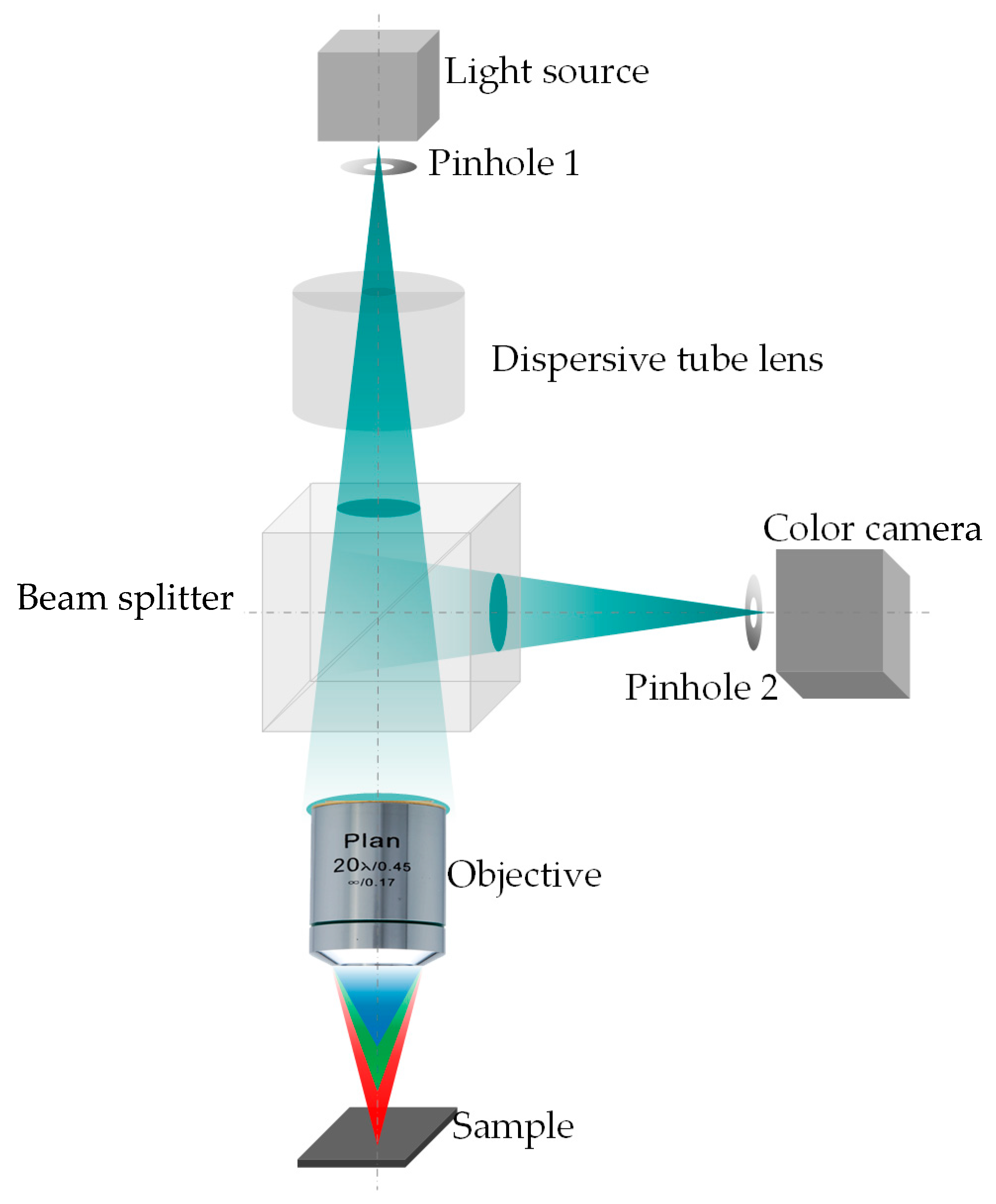
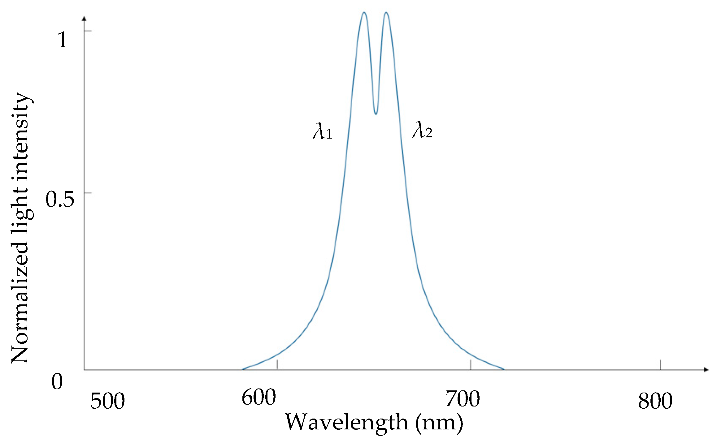
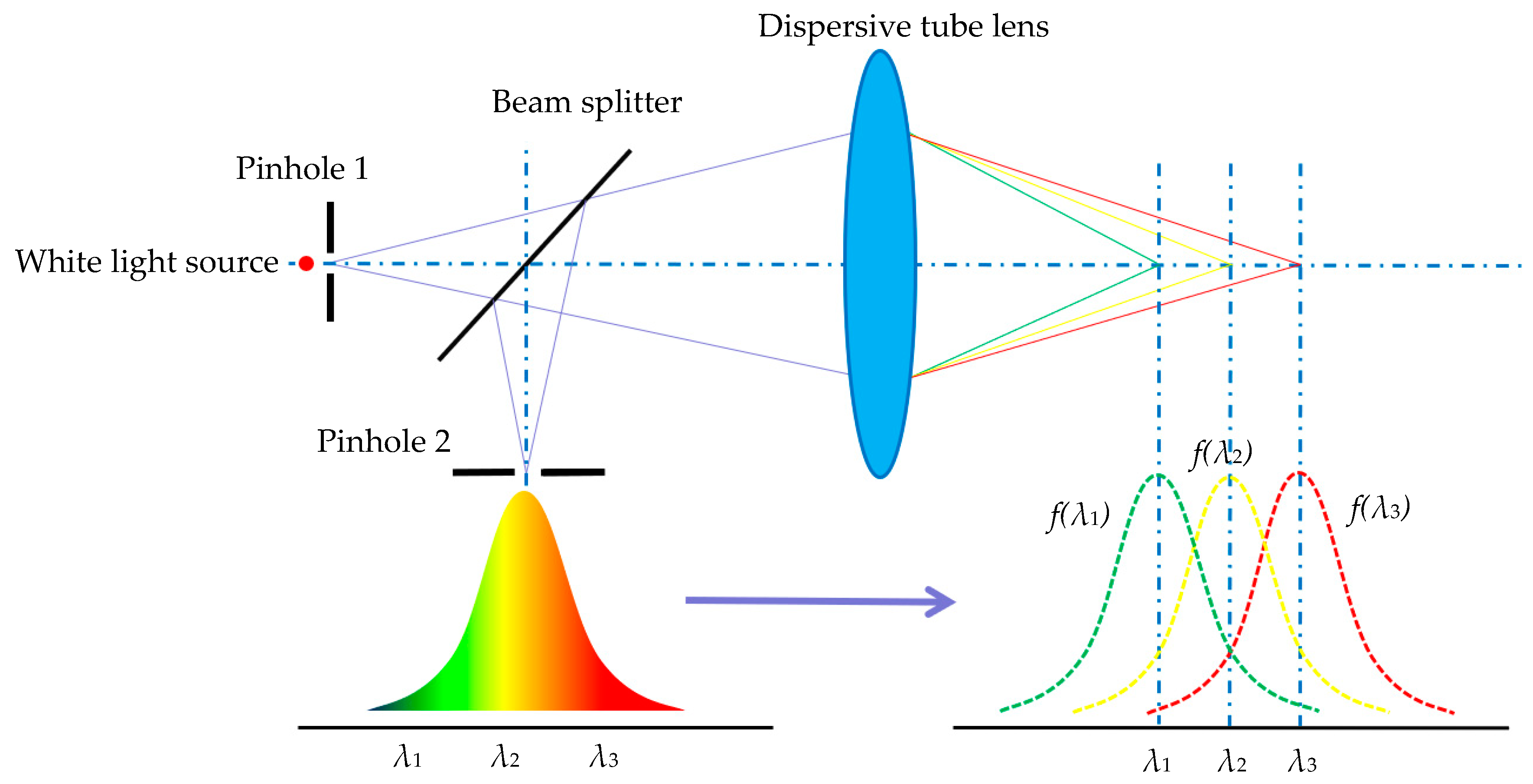
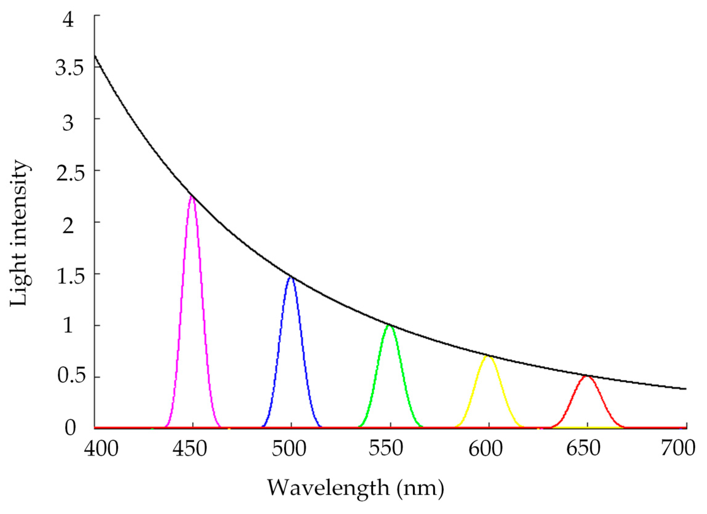
2.1.1. Principle of Chromatic Confocal Measurement

As a non-contact optical measurement method, chromatic confocal technology can obtain the surface topographic image of the specimen without mechanical axial scanning. The schematic diagram of chromatic confocal technology is shown in Figure 1. The polychromatic light beam emitted from the white light source passes through an illumination pinhole (pinhole 1 in Figure 1), which modulates the light beam into a point light. Then, the light beam with different wavelengths is distributed along the optical axis by the dispersion tube lens. The dispersed lights are then focused at the different axial positions by the objective. Being reflected by the specimen surface, only the light beam from the focal position can pass through the detection pinhole (pinhole 2 in Figure 1) and arrive at the detector with a peak intensity. By detecting the wavelength with a peak intensity, the height of the current measurement point can be determined.

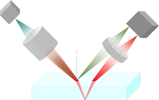
2.1.2. Principle of Chromatic Confocal Measurement with Inclined Illumination

In a conventional chromatic confocal measuring system, the optical axis is set to be perpendicular to the specimen surface, as mentioned in Section 2.1.1. When measuring a transparent specimen, it can capture the upper and lower surfaces by detecting two peaks of intensity. For thin sheet measurement, these two peaks may overlap to some extent, as shown in Figure 2. One of the solutions is to reduce the size of pinhole 2 to improve the detection sensitivity. However, the tradeoff is the weaker imaging light and higher alignment difficulty.

The other solution is to separate the imaging path from the illumination one, as shown in Figure 3.

In this design, the optical axis of the illumination path is not perpendicular to the specimen surface, as it is set in a conventional confocal system. Under this situation, the light beam from the light source, which is HL-2000-FHSA of the Ocean Optics, passes through a dispersive tube lens and reaches the upper surface. Then, the reflected light beams from the upper and lower surfaces of the specimen are focused at the different locations of the detector, and these two optical paths are parallel, instead of coaxial, to each other. In order to keep the confocal structure, a new conjugated relationship should be built for the illumination pinhole, the imaging focal point, and the detection pinhole. Because the imaging light is no longer coaxial, the method of point detection in the conventional chromatic confocal measurement system is not applicable in the proposed system. An inclined detection method is needed.

2.2. Theory of Chromatic Confocal Measurement with Inclined Illumination

2.2.1. Theoretical Analysis

According to the chromatic confocal microscope theory, a prototype with an inclined illumination was built, and the upper surface of the transparent specimen was set as the test specimen, as shown in Figure 3.

In the conventional chromatic confocal measurement technology, the normalized light intensity at the confocal pinhole can be expressed as follows:

$$I(u)={[\frac{\pi a^2}{\lambda f}sinc(\frac{u}{4})]}^4$$

(1)

where u is the normalized axial coordinate, λ is the wavelength of the incident light, a is the exit pupil radius of the imaging lens, and f represents the focal length of the lens. The normalized axial coordinate u can be expressed as follows:

$$u=\frac{2\pi }{\lambda }\Delta z\frac{a^2}{f^2}$$

(2)

In Equation (2), Δz is the defocusing amount, which is determined by the response function of axial light intensity in a chromatic confocal measurement system.

Equation (1) indicates that every light spot with a different wavelength corresponds to an axial light intensity response, which is largest at the position of the focused point, and decreases with the increasing of the defocusing amount, as shown in Figure 4.

In an ideal chromatic confocal system, the axial positions are linearly related to the wavelengths of the focused lights:

$$f({\lambda }_i)=h_0+k{\lambda }_i$$

(3)

where f(λ_i) represents the optical axial position, λ_i represents the wavelength of the focused light, and h₀ and k are constants. For a beam of light with a wavelength λ_i, the defocusing amount is as follows:

$$\Delta h=f({\lambda }_i)-f({\lambda }_0)=k({\lambda }_i-{\lambda }_0)$$

(4)

In Figure 3, the inclined angle between the optical axis of illumination path and the normal direction of the specimen surface is defined as θ. Thus, the relationship between the displacement of the focused point Δh and that of the specimen Δz(λ_i) can be expressed as follows:

$$\Delta z({\lambda }_i)=\Delta h·cos\theta$$

(5)

Substituting Equations (3)–(5) into Equation (1), the light intensity response function of any wavelength at the focused point is shown as follows:

$$I({\lambda }_i)={[\frac{\pi a^2}{{\lambda }_i(h_0+k{\lambda }_i)}sinc(\frac{\pi a^{2}k({\lambda }_i-{\lambda }_0)cos\theta }{2{\lambda }_i{(h_0+k{\lambda }_i)}^2})]}^4$$

(6)

The light intensity distribution of Equation (6) is simulated, which is shown in the black curve in Figure 5. The curve consists of all the peak points of light intensity at every wavelength from 400–700 nm, and each curve at every wavelength can be calculated and plotted with the conventional laser confocal formula, as shown in Equation (7). To understand the axial intensity distribution of the chromatic confocal system easily, several groups of light intensity curves at wavelengths of 450 nm, 500 nm, 550 nm, 600 nm, and 650 nm were simulated, as shown in the curves with different colors in Figure 5.

$$I(z)={[\frac{sin(\frac{u^{\prime }}{4})}{\frac{u^{\prime }}{4}}]}^4$$

(7)

where u′ is the normalized axial optical coordinate, which can be expressed as follows:

$$u^{\prime }=\frac{2\pi }{\lambda }z\frac{a^2}{f^2}$$

(8)

As mentioned above, the wavelength detected with the peak intensity is related to the axial position of the light spot in the chromatic confocal system, as a result, the chromatic confocal system with inclined illumination also has good spectral frequency selection characteristics.

2.2.2. Thickness Calculation Model in the Chromatic Confocal System with Inclined Illumination

In Section 2.1.2, the theoretical model of the proposed system was analyzed. In this section, the thickness calculation model for a transparent specimen is discussed.

As shown in Figure 6, there are two wavelength components (λ₀ and λ_i) focused on the upper and lower surfaces, with the focal points of O and B, respectively. If there was no test specimen, the light beam with wavelength λ_i would be focused at point C.

The thickness of the transparent specimen d can be expressed as follows:

$$d=OA·cos\theta ·\frac{(tan\alpha -tan\beta )}{(tan{\alpha }^{\prime }-tan{\beta }^{\prime })}$$

(9)

Substituting Equation (4) into Equation (9),

$$d=k({\lambda }_i-{\lambda }_0)·cos\theta ·\frac{(tan\alpha -tan\beta )}{(tan{\alpha }^{\prime }-tan{\beta }^{\prime })}$$

(10)

α and β can be calculated by θ and δ:

$$\{\begin{array}{l}\alpha =\theta +\delta \\ \beta =\theta -\delta \end{array}$$

(11)

δ is related to the diameter of the dispersion tube lens and the distance between point C and the dispersion tube lens. In the author’s system, these two values are a and h₀, respectively. Thus, δ can be expressed by the following:

$$\delta =arctan[\frac{a}{2(h_0+k{\lambda }_i)}]$$

(12)

Finally, in order to make the expression more concise, Equation (10) is preserved. However, as in the analysis mentioned above, for the actual calculation of thickness, Equations (11) and (12) are both necessary.

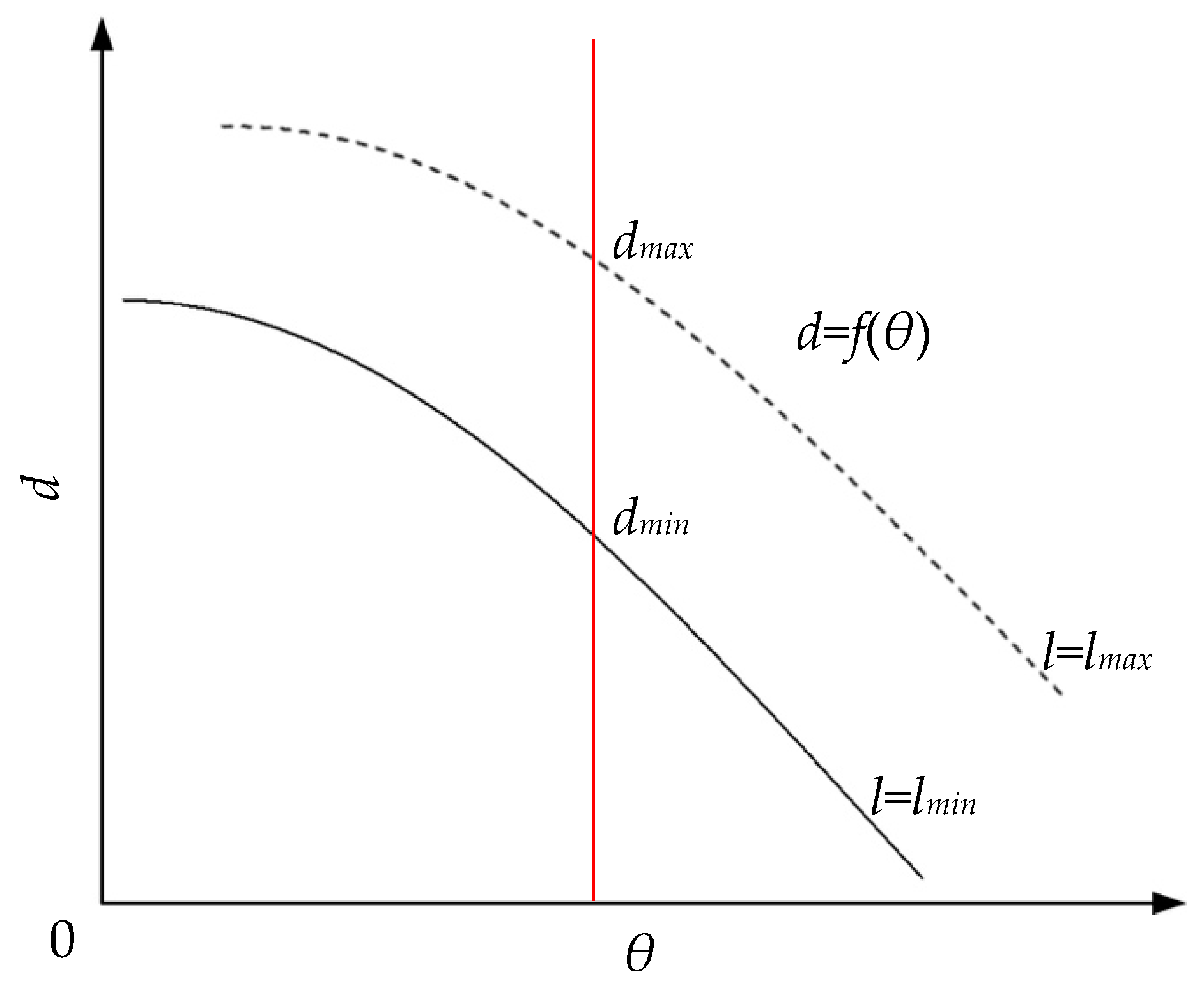
2.2.3. Analysis for the Influence of θ on Measurement Range of Thickness

In this proposed chromatic confocal model, the inclined angle θ is critical. Therefore, the relationship between the thickness d and the angle θ is worth discussion. As shown in Figure 6, there is a geometric relationship between the thickness d and the angle θ, which can be expressed as follows:

$$d=PB=\frac{OP}{{sin\theta }^{\prime }}=\frac{n_1·l·sin\theta }{tan(arcsin(\frac{sin\theta }{n_2}))}$$

(13)

In our system, n₁ is 1. Based on Equation (13), the curves of d can be plotted as Figure 7.

There are two curves in Figure 7. The curve with a solid line and dotted line represent the minimum and maximum thickness that the system can measure, respectively. Obviously, both curves will decrease as the angle θ increasing. Now, if the angle θ is fixed, as shown with the red line in Figure 7, we will get d_max and d_min. As indicated by Equation (13), d_max and d_min are both decided by l. Therefore, it is necessary to discuss the value range of l. There are two light spots with red and green in Figure 6, which are reflected by the upper and lower surfaces, respectively. When these two light spots are circumscribed, they can be distinguished, and l has the minimum value, as follows:

$$l_{min}=2r$$

(14)

r represents the radius of the light spot.

As the thickness of the transparent specimen increases, the distance between the light spots received by the detector will also increase. However, the size of the detector is limited, so when these two light spots arrive at the edge of the detector seperately, l has the maximum value:

$$l_{max}=D-2r$$

(15)

D represents the imaging size of the detector.

Considering the specific parameters of the experimental device, such as the linear range of the dispersive tube lens, the maximum and minimum values of l can be obtained. The dispersive tube lens is developed in house, and its linear range is known as 1100 μm, which is smaller than D − 2r. Combining those quantities in Section 3.1.1, the values of d_min and d_max can be calculated.

2.2.4. Color Conversion Algorithm

The images collected by the color camera contain R, G, and B values, which make the images show different colors. As discussed in the above sections, the axial displacement of the specimen is related to the wavelength detected with the peak intensity. However, the wavelength value cannot be directly obtained through the RGB image. Thus, a conversion algorithm is needed to translate the color information into wavelength values. The wavelength information can be obtained by converting the RGB space into the HSI space, in which the H value is directly related to the wavelength. This conversion is shown in Figure 8:

In the HSI space, H can be expressed as follows:

$$H=\{\begin{array}{ll}\theta ,& G\ge B\\ 2\pi -\theta ,& G<B\end{array}$$

(16)

where $\theta =co{s}^{-1}(\frac{(R-G)+(R-B)}{2\sqrt{{(R-G)}^2+(R-B)(G-B)}})$

Using Equation (16), the R, G, and B information obtained by the color camera can be converted to H value. Therefore, Equation (3) will become the following:

$$f(H_i)=h_1+k_1{H}_i$$

(17)

The thickness of the transparent specimen d becomes the following:

$$d=k_1(H_i-H_0)·cos\theta ·\frac{(tan\alpha -tan\beta )}{(tan{\alpha }^{\prime }-tan{\beta }^{\prime })}$$

(18)

3. Experimental Analysis

3.1. Setup and Calibration Experiment of the System

3.1.1. The Selection of Angle θ

As mentioned in Section 2.2.3, l_min and l_max can be calculated through the size of light spot, the size of detector and the linear range of the dispersive tube lens. In the experiments, thicknesses of specimens were about 180 μm and 1000 μm, respectively; so the d_min and d_max were set as 50 and 1100 μm, respectively. Therefore, the angle θ can be calculated as 39° by Equation (13).

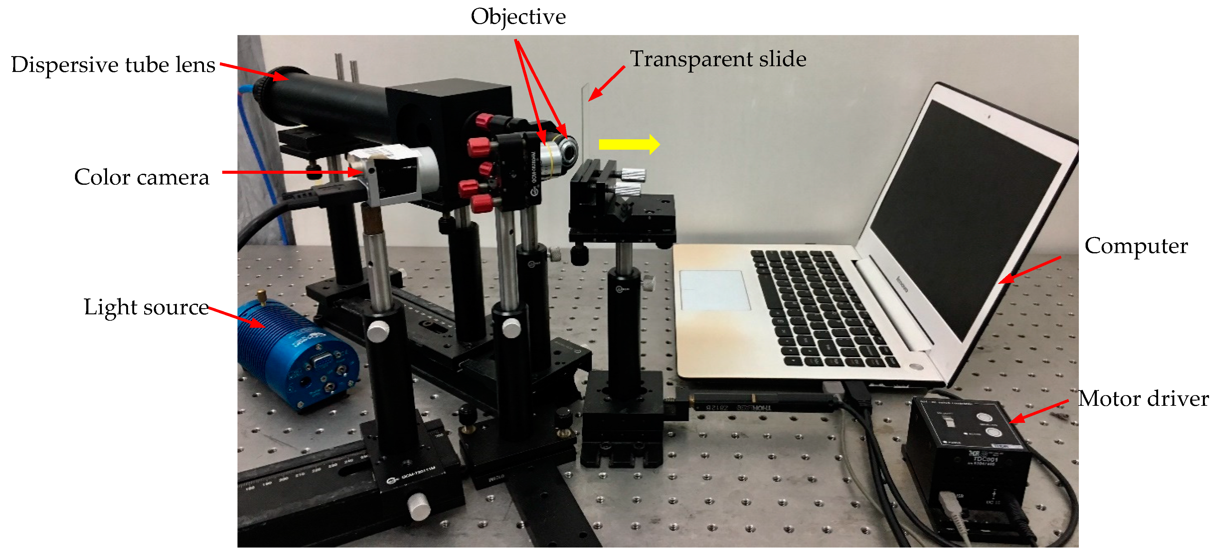
3.1.2. Setup of the System

Based on these theory analyses mentioned above, a chromatic confocal measurement device with inclined illumination was built, as shown in Figure 9. In this measurement device, an in-house developed dispersion tube lens was used to produce axial dispersion, and two objectives were placed before the specimen. The parameters of the two objectives are shown in

Table 1. The parameters of the objectives.

Objective Parameters	Value
magnification	10×
N.A. value	0.2

. The motor diver is the T-Cube DC Servo Controller (TDC001), which is used to push the transparent specimen in the direction of the yellow arrow shown in Figure 9. The computer is used to control the movement of the motor and is also used to connect the camera to get the RGB image. In the detection part, a color camera is applied as the receiver, whose model is Balser acA2440-35uc.

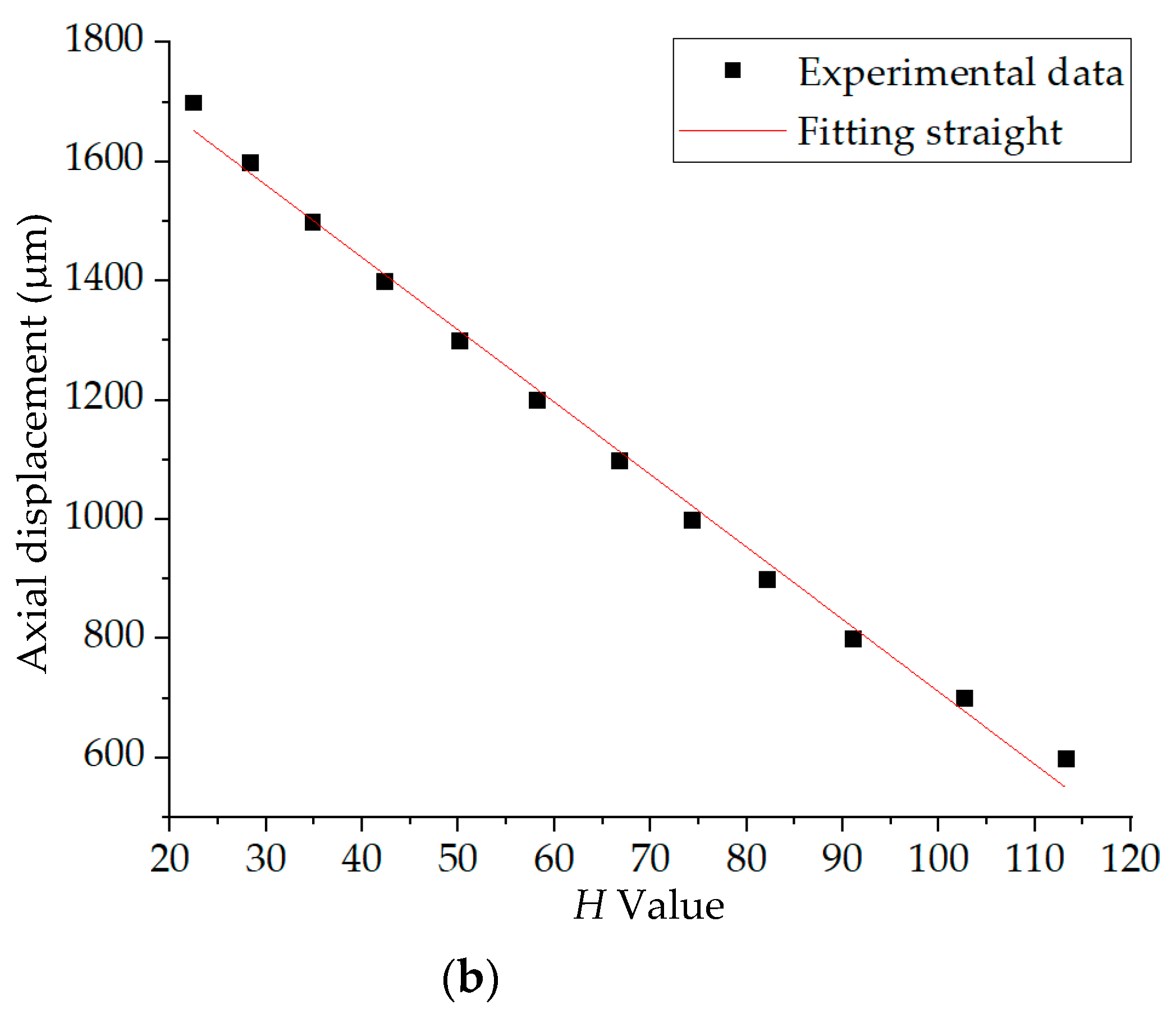
3.1.3. Calibration Experiment of the System

To establish the relationship between the position of the specimen surface and the information of the image color, a calibration experiment was performed in this system. A slide was used as the specimen in the experiment. The data of 16 positions along the yellow arrow were recorded, as shown in Figure 10. The images were captured by the color camera and converted to H values by the in-house developed color conversion algorithm in Section 2.2.4.

In Figure 9, as the measured transparent specimen gradually moves away from the objective, the color received by the color camera will gradually change from green to red. As shown in Figure 10, 16 groups of pictures were captured in the calibration experiment that could indicate the color change from the upper and lower surfaces of the transparent glass slide in the whole calibration process. In the author’s system, a circle with a diameter of 100 pixels was selected as the “pinhole”. Thus, the average H value of the circle in the center of one picture was calculated to characterize the whole light spot. Figure 10 shows the pixel-processed calibration image, which is a circle with a diameter of 100 pixels. “The lower” in Figure 10 represents the color change reflected from the lower surface of the transparent specimen, and “the upper” represents the color change reflected from the upper surface of the transparent specimen. In the calibration experiment, only the images from the upper surface of the slide were recorded and processed.

The average H values of these 16 light spots in Figure 10 were calculated, and the axial displacement was measured by the inductance micrometer Tesa TT80. The calibration curve before fitting is shown in Figure 11a. Within 600–1700 μm, 12 points were selected for fitting. The experimental data are presented in

Table 2. Calibration result calculated using the data from the upper surface of the slide.

Axial Displacement (μm)	H Value
1700.00	22.41
1600.00	28.26
1500.00	34.78
1400.00	42.24
1300.00	50.11
1200.00	58.11
1100.00	66.66
1000.00	74.32
900.00	82.11
800.00	91.04
700.00	102.65
600.00	113.16
500.00	119.32
400.00	123.91

and the linear fitting result is plotted in Figure 11b.

In the linear fitting, the standard square value of the fitting curve was 0.99, and the relationship between the axial displacement of the slide f(H) and the H value is as below:

$$f(H)=1924.90-12.14H$$

(19)

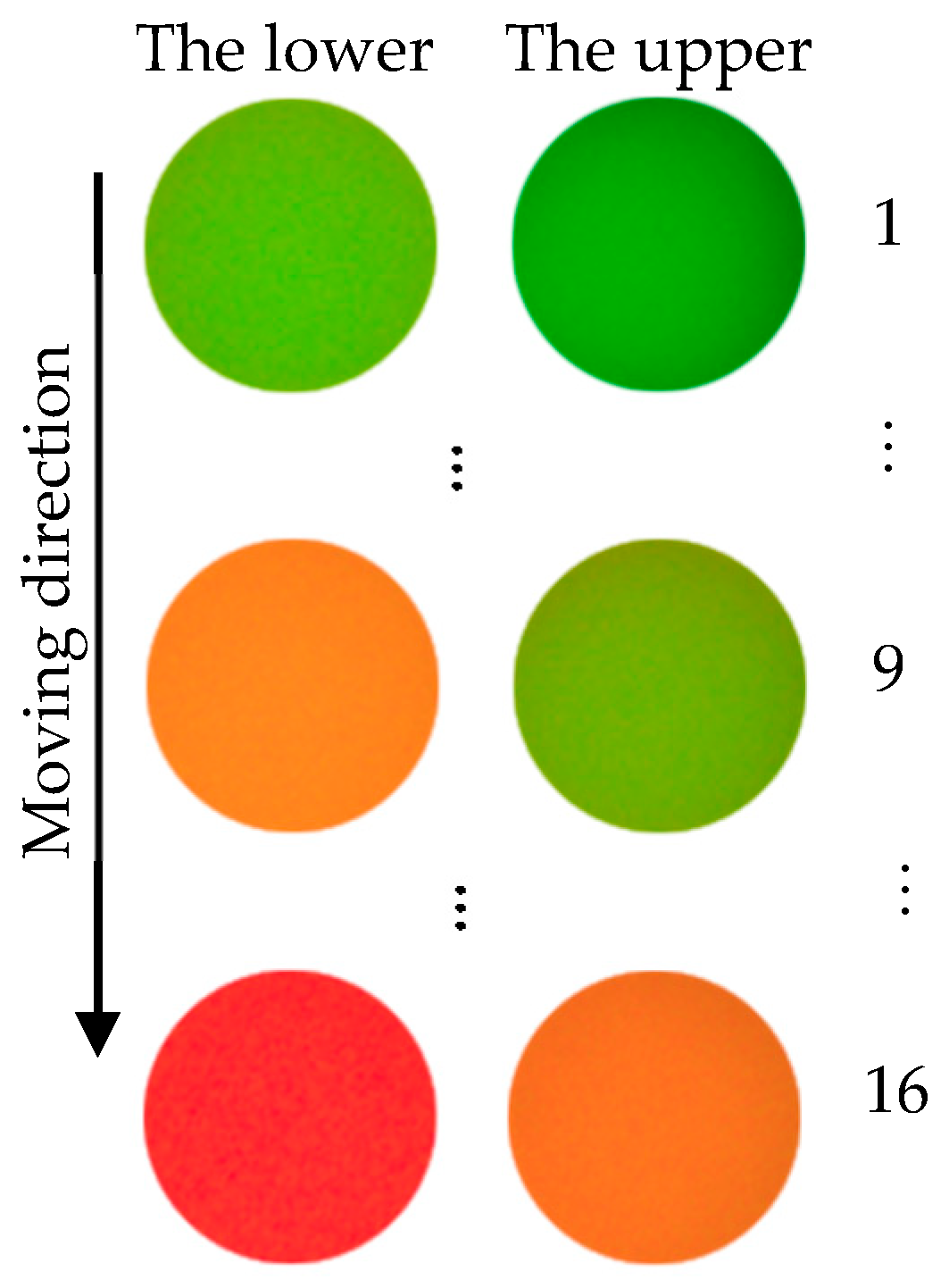
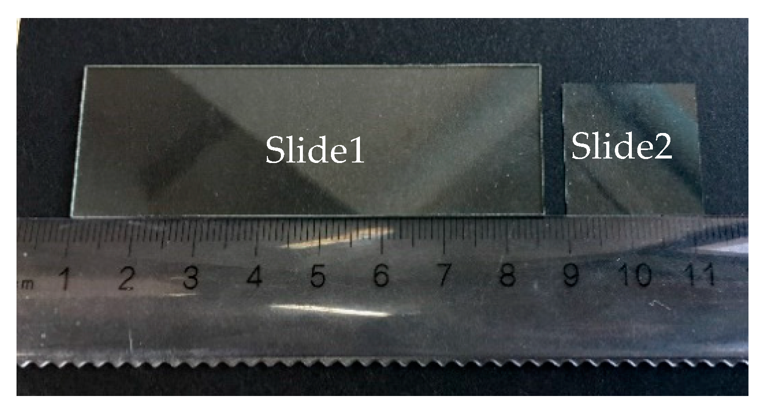
3.2. Thickness Measurement for Transparent Specimen

In Section 2.2.2, the calculation formula for the thickness of the transparent specimen has been proposed. Using the experimental platform shown in Figure 9, the calibration work was performed. Then, two kinds of transparent glass slides with different thicknesses were measured. The physical images of Slide 1 and Slide 2 are shown in Figure 12. The transmission of the two transparent glasses used in this experiment ranged from 84% (at 380 nm) to 90% (at 717 nm).

(a)

Slide 1: thicker transparent specimen

The true value of Slide 1 was 973.28 μm, which was measured by the inductance micrometer. In the calibration experiment, two reflected light spots from the upper and lower surface of the slide could be achieved, of which the upper ones were used to calibrate the system. H_i and H₀ of these two light spots were calculated by Equation (16). As the slide moves along the yellow arrow in Figure 9, several groups of H_i and H₀ values can be obtained; however, the differences in each group, which can be represented as H_i-H₀, are not equal. Considering Equation (18), it is known that the thickness of the slide is not only related to the difference between H_i and H₀, but also related to the initial parameters of the measurement system. Therefore, the axial position of the slide along the yellow arrow was fixed. At this axial position, θ, a, and h₀ were each measured first, and then δ was calculated through Equation (12), which was 19.1°. The other parameters in Equation (18) are listed in

Table 3. Fixed parameters in Equation (18).

Parameter	Value
α	58.10°
β	19.90°
α′	34.50°
β′	13.10°
θ	39.00°

.

The experiments of the thickness measurement were repeated 40 times; Figure 13 shows one of the 40 captured pictures in the measurement of Slide 1.

Using the color conversion algorithm introduced in Section 2.2.4, the R, G, and B information of these 40 pieces of pictures were converted to H values, as listed in

Table 4. Experimental data of the thickness of Slide 1.

Piece Number	H Value of Upper Surface	H Value of Lower Surface	Value of Difference	Piece Number	H Value of Upper Surface	H Value of Lower Surface	Value of Difference
1	24.45	63.02	38.57	21	24.45	63.11	38.66
2	24.49	62.75	38.25	22	24.49	63.37	38.89
3	24.46	63.13	38.67	23	24.06	63.10	39.04
4	24.49	63.10	38.60	24	24.49	63.14	38.64
5	24.47	63.13	38.66	25	24.07	63.16	39.09
6	24.50	63.01	38.52	26	24.45	63.11	38.66
7	24.46	63.11	38.66	27	24.49	63.06	38.57
8	24.49	63.12	38.63	28	24.45	63.08	38.63
9	24.48	63.08	38.59	29	24.49	63.11	38.62
10	24.46	63.16	38.70	30	24.46	63.10	38.63
11	24.49	62.94	38.45	31	24.49	63.05	38.56
12	24.49	63.17	38.69	32	24.49	63.40	38.91
13	24.46	63.01	38.55	33	24.45	63.12	38.67
14	24.48	63.13	38.65	34	24.48	63.13	38.65
15	24.49	63.01	38.51	35	24.49	63.37	38.87
16	24.45	63.18	38.73	36	24.50	63.07	38.57
17	24.49	62.96	38.47	37	24.45	63.09	38.64
18	24.07	63.15	39.09	38	24.49	63.12	38.63
19	24.49	62.96	38.47	39	24.48	63.09	38.61
20	24.07	63.20	39.12	40	24.46	63.14	38.68
The average value of the difference		38.67		Relative error (σ)		0.18

.

Based on the discussion in Section 2.2.3 and Section 3.1.1, θ was determined as 39°, and the value of k₁ is 12.14 expressed in Equation (18). Calculated with the data in Table 4 and

Table 5. Experimental data of the thickness of Slide 2.

Piece Number	H Value of Upper Surface	H Value of Lower Surface	Value of Difference	Piece Number	H Value of Upper Surface	H Value of Lower Surface	Value of Difference
1	52.07	59.49	7.42	21	52.03	59.48	7.45
2	52.02	58.91	6.89	22	52.08	59.44	7.36
3	52.09	59.51	7.42	23	52.03	59.36	7.32
4	52.05	58.90	6.85	24	52.09	59.45	7.35
5	52.05	59.40	7.35	25	52.12	59.40	7.29
6	52.06	58.57	6.51	26	52.09	59.40	7.32
7	52.08	59.51	7.43	27	52.04	59.48	7.44
8	52.04	58.88	6.84	28	52.06	59.50	7.43
9	52.06	59.44	7.38	29	52.05	58.98	6.93
10	52.06	59.40	7.34	30	52.07	59.52	7.45
11	52.07	59.47	7.41	31	52.06	59.44	7.37
12	52.08	58.95	6.87	32	52.07	59.48	7.41
13	52.05	59.50	7.44	33	52.10	59.45	7.34
14	52.01	58.94	6.93	34	52.07	59.45	7.38
15	52.07	59.41	7.34	35	52.05	58.91	6.86
16	52.07	58.90	6.83	36	52.12	59.49	7.37
17	52.09	59.46	7.37	37	52.08	59.43	7.35
18	52.10	59.47	7.37	38	52.06	59.46	7.40
19	52.07	59.45	7.37	39	52.04	58.95	6.91
20	52.04	58.96	6.91	40	52.09	59.50	7.41
The average value of the difference		7.24		Relative error (σ)		0.25

with Equation (18), the thickness of Slide 1 was 998.82 μm. The calculation formula of σ is as follows:

$$\sigma =\sqrt{\frac{{\displaystyle \sum {\left(x_i-\overline{x}\right)}^2}}{n-1}}$$

(20)

The repeatability was 0.54μm, measured by 3σ, and the measurement error was 2.62%.

(b)

Slide 2: thinner transparent specimen

Based on the measurement of the thicker slide in part (a), the measurement of the 170–190 μm slide was carried out. The experiments of the thickness measurement were also repeated 40 times; Figure 14 shows one of the 40 captured pictures in the measurement of Slide 2.

The true value of Slide 2 is 181.08 μm, measured by the inductance micrometer. The results were measured by the self-built instrument and are listed in Table 5.

The data in Table 5 were processed in the same way as for Slide 1, and the thickness was calculated to be 187.00 μm. The repeatability was 0.75 μm, measured by 3σ, and the measurement error was 3.27%.

4. Discussions

The experimental results showed that the axial measurement accuracy of the system could reach the micron level and the repeatability is better than 0.75 μm. However, there is a high requirement for the position of all the optical parts in this system, and we will try to improve the adaptability of the system in future works.

The relationship between the thickness d and the angle θ is discussed and derived in this paper. We calculate the value of θ through the values of d_min and d_max, which is 39°.

The transmission of the two transparent glass slides used in this experiment ranged from 84% to 90%. The current experiments have requirements for the transmission, flatness of transparent specimens, and the stability of the measuring system. In the future, related studies and quantificational analyses will be conducted for different materials.

The application scope of this paper is mainly the measurement of transparent specimens. In the future, not only the relationship of inclined angle θ and thickness measurement range, but also the influence of attenuation range and refractive index of transparent specimens in the system, will be further discussed.

5. Conclusions

In this paper, a novel chromatic confocal system with inclined illumination is proposed. The mathematic model of the thickness measurement for the transparent specimens was built, and the influence of the inclined angle θ was discussed. The experimental results show that the axial measurement accuracy reached the micron level and the repeatability was better than 0.75 μm.

References

1. Wang, Y.; Xi, M.; Liu, H.; Ding, Z.; Du, W.; Meng, X.; Sui, Y.; Li, J.; Jia, Z. On-machine noncontact scanning of high-gradient freeform surface using chromatic confocal probe on diamond turning machine. Opt. Laser Technol. 2021, 134, 106569. [Google Scholar] [CrossRef]
2. Hillenbrand, M.; Lorenz, L.; Kleindienst, R.; Grewe, A.; Sinzinger, S. Spectrally multiplexed chromatic confocal multipoint sensing. Opt. Lett. 2013, 38, 4694–4697. [Google Scholar] [CrossRef]
3. Chun, B.; Kim, K.; Gweon, D. Three-dimensional surface profile measurement using a beam scanning chromatic confocal microscope. Rev. Sci. Instrum. 2009, 80, 073706. [Google Scholar] [CrossRef] [Green Version]
4. Du, H.; Zhang, W.; Ju, B.; Sun, Z.; Sun, A. A new method for detecting surface defects on curved reflective optics using normalized reflectivity. Rev. Sci. Instrum. 2020, 91, 036103. [Google Scholar] [CrossRef]
5. Zou, J.; Yu, Q.; Cheng, F. Differential chromatic confocal roughness evaluation system and experimental research. Chin. Opt. 2020, 13, 1103–1114. [Google Scholar]
6. Fu, S.; Kor, W.S.; Cheng, F.; Seah, L.K. In-situ measurement of surface roughness using chromatic confocal sensor. Procedia CIRP 2020, 94, 780–784. [Google Scholar] [CrossRef]
7. Berkovic, G.; Zilberman, S.; Shafir, E.; Rubin, D. Chromatic confocal displacement sensing at oblique incidence angles. Appl. Opt. 2020, 59, 3183–3186. [Google Scholar] [CrossRef] [PubMed]
8. Bai, J.; Li, X.; Wang, X.; Zhou, Q.; Ni, K. Chromatic Confocal Displacement Sensor with Optimized Dispersion Probe and Modified Centroid Peak Extraction Algorithm. Sensors 2019, 19, 3592. [Google Scholar] [CrossRef] [PubMed] [Green Version]
9. Chen, C.; Wang, J.; Liu, X.; Lu, W.; Zhu, H.; Jiang, X. Influence of sample surface height for evaluation of peak extraction algorithms in confocal microscopy. Appl. Opt. 2018, 57, 6516–6526. [Google Scholar] [CrossRef] [PubMed]
10. Sun, H.; Wang, S.; Bai, J.; Zhang, J.; Huang, J.; Zhou, X.; Liu, D.; Liu, C. Confocal laser scanning and 3D reconstruction methods for the subsurface damage of polished optics. Opt. Lasers Eng. 2021, 136, 106315. [Google Scholar] [CrossRef]
11. Hillenbrand, M.; Weiss, R.; Endrody, C.; Grewe, A.; Hoffmann, M.; Sinzinger, S. Chromatic confocal matrix sensor with actuated pinhole arrays. Appl. Opt. 2015, 54, 4927–4936. [Google Scholar] [CrossRef] [PubMed]
12. Luo, D.; Taphanel, M.; Claus, D.; Boettcher, T.; Osten, W.; Längle, T.; Beyerer, J. Area scanning method for 3D surface profilometry based on an adaptive confocal microscope. Opt. Lasers Eng. 2020, 124, 105819. [Google Scholar] [CrossRef]
13. Li, S.; Liang, R. DMD-based three-dimensional chromatic confocal microscopy. Appl. Opt. 2020, 59, 4349–4356. [Google Scholar] [CrossRef] [PubMed]
14. Hillenbrand, M.; Mitschunas, B.; Brill, F.; Grewe, A.; Sinzinger, S. Spectral characteristics of chromatic confocal imaging systems. Appl. Opt. 2014, 53, 7634–7642. [Google Scholar] [CrossRef] [PubMed]
15. Lu, W.; Chen, C.; Wang, J.; Richard, L.; Zhang, C. Characterization of the displacement response in chromatic confocal microscopy with a hybrid radial basis function network. Opt. Express 2019, 27, 22737–22752. [Google Scholar] [CrossRef] [PubMed]
16. Bai, J.; Li, X.; Wang, X.; Wang, J.; Ni, K.; Zhou, Q. Self-reference dispersion correction for chromatic confocal displacement measurement. Opt. Lasers Eng. 2021, 140, 106540. [Google Scholar] [CrossRef]
17. Miks, A.; Novak, J.; Novak, P. Analysis of method for measuring thickness of plane-parallel plates and lenses using chromatic confocal sensor. Appl. Opt. 2010, 49, 3259–3264. [Google Scholar] [CrossRef]
18. Boettcher, T.; Gronle, M.; Osten, W. Single-shot multilayer measurement by chromatic confocal coherence tomography. Opt. Metrol. 2017, 10329, 103290K. [Google Scholar]
19. Yu, Q.; Zhang, K.; Cui, C.; Zhou, R.; Cheng, F.; Ye, R.; Zhang, Y. Method of thickness measurement for transparent specimens with chromatic confocal microscopy. Appl. Opt. 2018, 57, 9722–9728. [Google Scholar] [CrossRef]
20. Li, J.; Zhao, Y.; Du, H.; Zhu, X.; Wang, K.; Zhao, M. Adaptive modal decomposition based overlapping-peaks extraction for thickness measurement in chromatic confocal microscopy. Opt. Express 2020, 28, 36176–36187. [Google Scholar] [CrossRef]
21. Taphanel, M.; Beyerer, J. Fast 3D In-line Sensor for Specular and Diffuse Surfaces Combining the Chromatic Confocal and Triangulation Principle. In Proceedings of the Conference Record IEEE Instrumentation & Measurement Technology Conference, Graz, Austria, 13–16 May 2012. [Google Scholar]
22. Taphanel, M.; Zink, R.; Längle, T.; Beyerer, J. Multiplex acquisition approach for high speed 3D measurements with a chromatic confocal microscope. SPIE Opt. Metrol. 2015, 9525, 95250Y. [Google Scholar]
23. Seung, W.L.; Garam, C.; Sin, Y.L.; Yeongchan, C.; Heui, J.P. Coaxial spectroscopic imaging ellipsometry for volumetric thickness measurement. Appl. Opt. 2021, 60, 67–74. [Google Scholar]
Figure 1. Principle of the chromatic confocal measurement method.
Photonics 08 00170 g001
Figure 2. Overlap of the signals from the top and bottom surfaces of transparent specimen (λ1 and λ2 represent two different wavelengths, respectively).
Photonics 08 00170 g002
Figure 3. Separation of these two signals from the upper and lower surfaces of a transparent specimen (θ is the inclined angle between the optical axis of incident light and the normal direction of the specimen surface).
Photonics 08 00170 g003
Figure 4. Schematic diagram of the intensity response.
Photonics 08 00170 g004
Figure 5. Light intensity distribution with different wavelengths.
Photonics 08 00170 g005
Figure 6. Thickness calculation model of a transparent specimen. The letters in the picture represent the following meanings: n1: the refractive index of the air; n2: the refractive index of the transparent specimen; λ0: the wavelength of green light; λi: the wavelength of red light; h0+ kλ0: the distance between point O and the lens 1; h0+ kλi: the distance between point C and the lens 1; a: the diameter of lens 1; d: the thickness of the transparent specimen; D: the imaging size of detector imaging surface; r: the radius of the image spots; l: the center distance of the imaging spots; θ: the inclined angle of the system; θ: the inclined angle of the system after refraction; δ: the optical axis of incident light and light beam with wavelength λi; α: the incidence angle of the left light beam with wavelength λi; α: the refraction angle of the left light beam with wavelength λi; β: the incidence angle of the right light beam with wavelength λi; β: the refraction angle of the right light beam with wavelength λi.
Photonics 08 00170 g006
Figure 7. The relationship between the thickness d and the angle θ.
Photonics 08 00170 g007
Figure 8. Principle of color conversion algorithm. (a) RGB space; (b) HSI space.
Photonics 08 00170 g008
Figure 9. Diagram of the chromatic confocal system with inclined illumination.
Photonics 08 00170 g009
Figure 10. The color change of the calibration experiment.
Photonics 08 00170 g010
Figure 11. (a) Calibration experiment result. (b) Linear fitting result.
Photonics 08 00170 g011aPhotonics 08 00170 g011b
Figure 12. Picture of the transparent glass slides.
Photonics 08 00170 g012
Figure 13. Experimental picture of Slide 1.
Photonics 08 00170 g013
Figure 14. Experimental picture of Slide 2.
Photonics 08 00170 g014