Computing 3D Phase-Type Holograms Based on Deep Learning Method


1
Department of Precision Mechanical Engineering, Shanghai University, Shanghai 200444, China
2
Key Laboratory of Advanced Display and System Application, Ministry of Education, Shanghai 200072, China
*
Author to whom correspondence should be addressed.
Photonics 2021, 8(7), 280; https://0-doi-org.brum.beds.ac.uk/10.3390/photonics8070280
Submission received: 31 May 2021
/
Revised: 24 June 2021
/
Accepted: 3 July 2021
/
Published: 15 July 2021
(This article belongs to the Special Issue Holography)
Abstract
:Computer holography is a technology that use a mathematical model of optical holography to generate digital holograms. It has wide and promising applications in various areas, especially holographic display. However, traditional computational algorithms for generation of phase-type holograms based on iterative optimization have a built-in tradeoff between the calculating speed and accuracy, which severely limits the performance of computational holograms in advanced applications. Recently, several deep learning based computational methods for generating holograms have gained more and more attention. In this paper, a convolutional neural network for generation of multi-plane holograms and its training strategy is proposed using a multi-plane iterative angular spectrum algorithm (ASM). The well-trained network indicates an excellent ability to generate phase-only holograms for multi-plane input images and to reconstruct correct images in the corresponding depth plane. Numerical simulations and optical reconstructions show that the accuracy of this method is almost the same with traditional iterative methods but the computational time decreases dramatically. The result images show a high quality through analysis of the image performance indicators, e.g., peak signal-to-noise ratio (PSNR), structural similarity (SSIM) and contrast ratio. Finally, the effectiveness of the proposed method is verified through experimental investigations.
1. Introduction
Computer-generated holograms (CGHs) are widely used in various fields [1,2], since computational holography can not only record and reproduce the amplitude and phase of light waves comprehensively, but also has the advantages of low noise and high reproducibility [3]. It can also generate holograms of virtual objects, compared with traditional optical holography.
There are many methods to generate CGHs. Phase-only CGH is a better option for holographic displays in most cases, due to the higher optical efficiency of phase modulation. Moreover, the reconstruction results by using the phase-only liquid crystal-based SLMs could have no interference of conjugate image. The iterative methods have significant advantages in phase retrieval [4,5,6]. However, for CGH generation, there is an unavoidable problem with the iterative methods because they require a trade-off between computation time and image quality caused by the iterative process [7,8,9]. Non-iterative complex amplitude encoding methods have also been proposed to achieve fast CGH calculation with guaranteed imaging quality, such as the error diffusion method [10] and the double phase encoding method [11,12].
In recent years, deep learning has shown a significant impact in various fields [13]. It has also become a beneficial tool for computational holography and other optical imaging applications, where machine learning models represented by convolutional neural networks (CNNs) shown agreeable performance in modeling and calculating highly nonlinear mapping problems in constant calculation time [14,15]. Therefore, it is an excellent choice for fast and efficient processing of optical information (including fast CGH generation). Neural networks have also been successfully applied to digital holography [16], computational imaging [17,18,19], hologram generation [20,21,22,23,24], etc.
The currently implemented method, using generative adversarial networks (GAN) instead of the traditional point sources method (LUT) for generation of point cloud CGHs [20], has successfully reduced the computational load. In addition, a deep neural network based on the residual network structure [21] was used to generate the phase-only CGHs and the reconstructed images were of better quality than those generated by Gerchberg–Saxton (GS) algorithm [4]. However, the proposed residual network has been trained with only a single input plane and the results are only used for simple images, such as simple handwritten numbers. More recently, the generation of multi-plane holograms based on deep learning has been proposed [22]. The network takes multiple images of different planes as input and calculates complex holograms as output, reconstructing each input image at the corresponding plane, demonstrating the feasibility of generating multi-plane holograms based on deep learning. However, this method only shows the imaging quality of network generated CGH with binary-gray scale image as input of different planes. Therefore, this study needs further research in processing multi-plane complex images and its imaging quality.
In this paper, a convolutional neural network-based hologram generation method is proposed to obtain the phase-only holograms of complex multi-plane images. The reconstruction quality of holograms generated by a network that undergoes deep learning is greatly enhanced by a data-set type and combination strategy. Therefore, this network is able to train faster and more efficient for hologram generation. Thus, the model has the ability to calculate holograms of target image patterns in a non-iterative mode. This deep learning method allows for generating holograms of various types of images without learning specific objects and it can be further extended to generate holograms from single-plane images to multi-plane images.
In Section 2, the CGH algorithm and the network structure are introduced. In Section 3, the existing algorithm of CGH is compared with the algorithm of this paper in terms of calculation speed and imaging accuracy. Simulation results show that the neural network outperforms iterative ASM and produces holograms faster compared to iterative ASM. The image quality is also analyzed by calculating PSNR, SSIM and other parameters.
2. Basic Theories
2.1. Optical Principle
Treating the electric vector as a scalar in the fluctuation equation, the following equation is obtained [25]
where is the frequency of the light wave.
Let the distance between the diffraction plane and the observation plane be and and are the complex amplitudes of the light waves on the diffraction plane and the observation plane, respectively. In the frequency domain, their spectral functions are and , respectively. By using the inverse Fourier transform of the spectral function for the light wave on the observation plane after propagation at distance , one obtains . Since and are the Fourier transforms of and respectively, and is the inverse Fourier transform of , one can see that
where is an imaginary unit and must satisfy the Helmholtz equation at all source-free points. With direct application of this requirement to Equation (2), after calculation and collation, we obtain a differential equation that satisfies
where is the wavelength and since is necessarily a special solution of the equation corresponding to = 0, according to the theory of differential equations, the solution of Equation (3) can be written as
The relationship for the spectral variation of the light wave field propagating from the diffraction plane to the observation plane is obtained. This relation shows that the propagation of the light wave along the -direction results in the frequency domain as the spectrum of the light wave field on the diffraction plane is multiplied by a -dependent phase delay factor . In the theory of linear systems, this phase delay factor, called the transfer function of diffraction in the frequency domain, is noted as . It indicates that the diffraction problem can be considered as a transformation process of the optical wavefield through a linear space-invariant system.
According to the angular spectrum theory of light propagation [26], the spectra of can be derived from the spectrum of complex amplitude by Equation (4) and the complex amplitude of the light wave at any observed position behind the diffraction plane can be further derived by inverse Fourier transform. The calculation process can be expressed by the Fourier transform as
In further processing of 3D objects, the above equation for single-plane 2D object surface can be expanded for 3D objects with different depth planes [27].
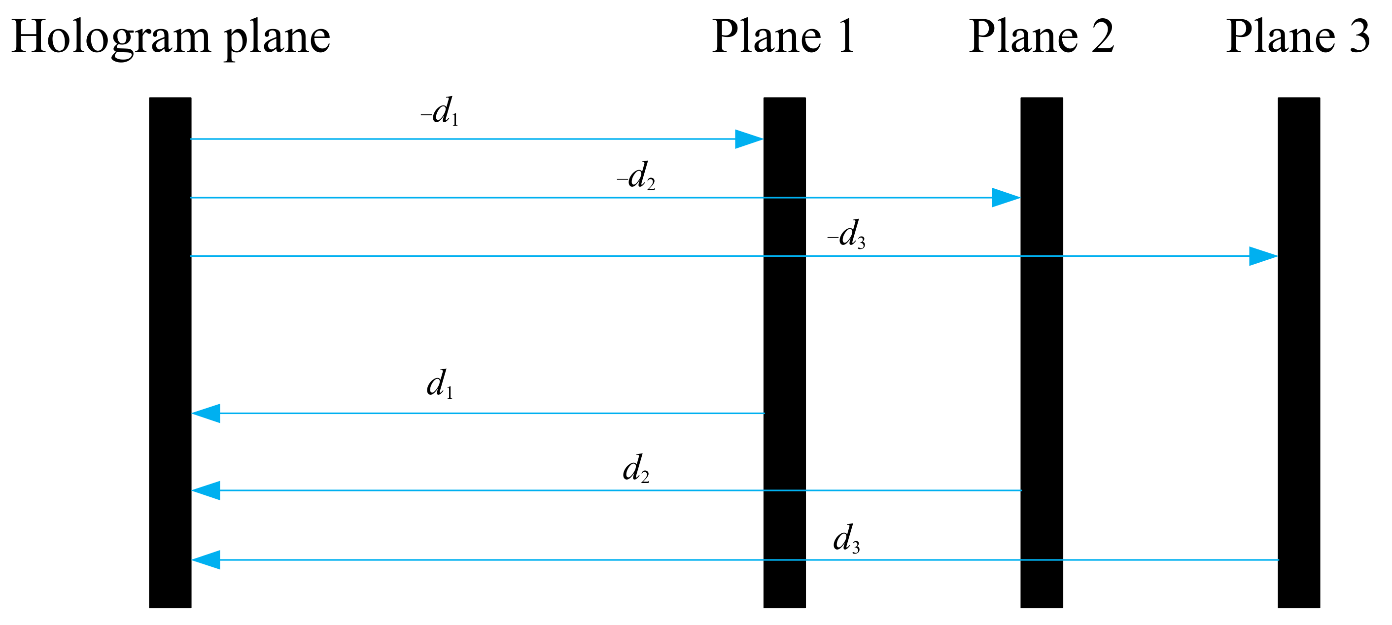
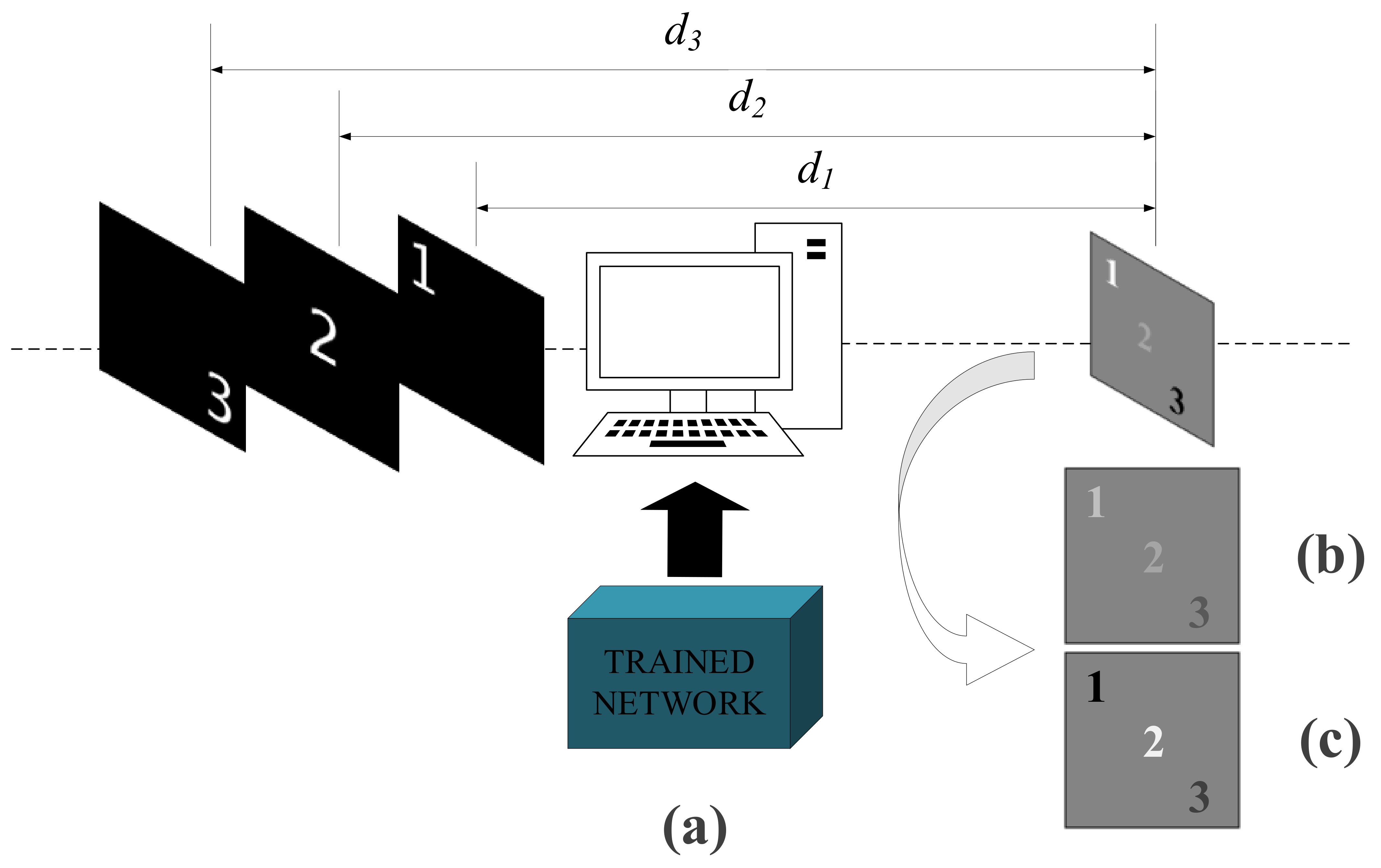
As shown in Figure 1, the light wave of object planes 1, 2, and 3 are diffracted to the hologram plane to form a hologram and then the light wave modulated by the resulting hologram is diffracted back to each object plane and the image can be reconstructed. With amplitude constraints, the light wave of each depth plane is diffracted again to hologram plane to obtain the renewed hologram in a cyclically iteration process. The complex hologram will be gradually converged to phase-only hologram of the multi-plane 3D object.
2.2. Neural Network Algorithm and Its Training Strategy
The algorithm in this paper takes multiple target images as inputs, with each image corresponding to each plane. The trained network obtains its complex amplitude in the hologram plane and then propagates it back to the object plane using the Fourier inversion (Equation (5)) in order to complete the hologram generation and reconstruction.
For simplicity, the number of input planes is set to three and the input planes are located at a distance of di (i = 1, 2, 3) from the hologram plane. That is, the light wave of multiple input images is back-propagated to the hologram plane and then the complex amplitude generated by superposition is divided into real part and imaginary part as the ground-truth data. The free-space propagation method is the multi-plane iterative ASM [28,29,30].
To effectively train a deep learning network, a well-organized training set is constructed and a network structure is designed. In order to construct the training set, the output data of the network and the target data need to be compared. The holograms with complex wavefront information make it difficult to intuitively find the corresponding relationships between the target data and the input data. This undoubtedly increases the training difficulty of the network. If the target data can be converted into more intuitive data with clearer correspondence, then the training difficulty will be greatly reduced. Moreover, the ability of the network to generate holograms will be more accurate and faster. A similar approach of training by intermediate variables instead of its original target data has been validated by Ketao Yan et al. [31], using convolutional neural networks in wrapped bit-phase denoising. During the training process, the model can calculate holograms quickly within a predicable time window which only depends on the model size (number of convolutional layers, number of kernels, kernel size), the number of model iterations, the number of depth planes and the size of the hologram.
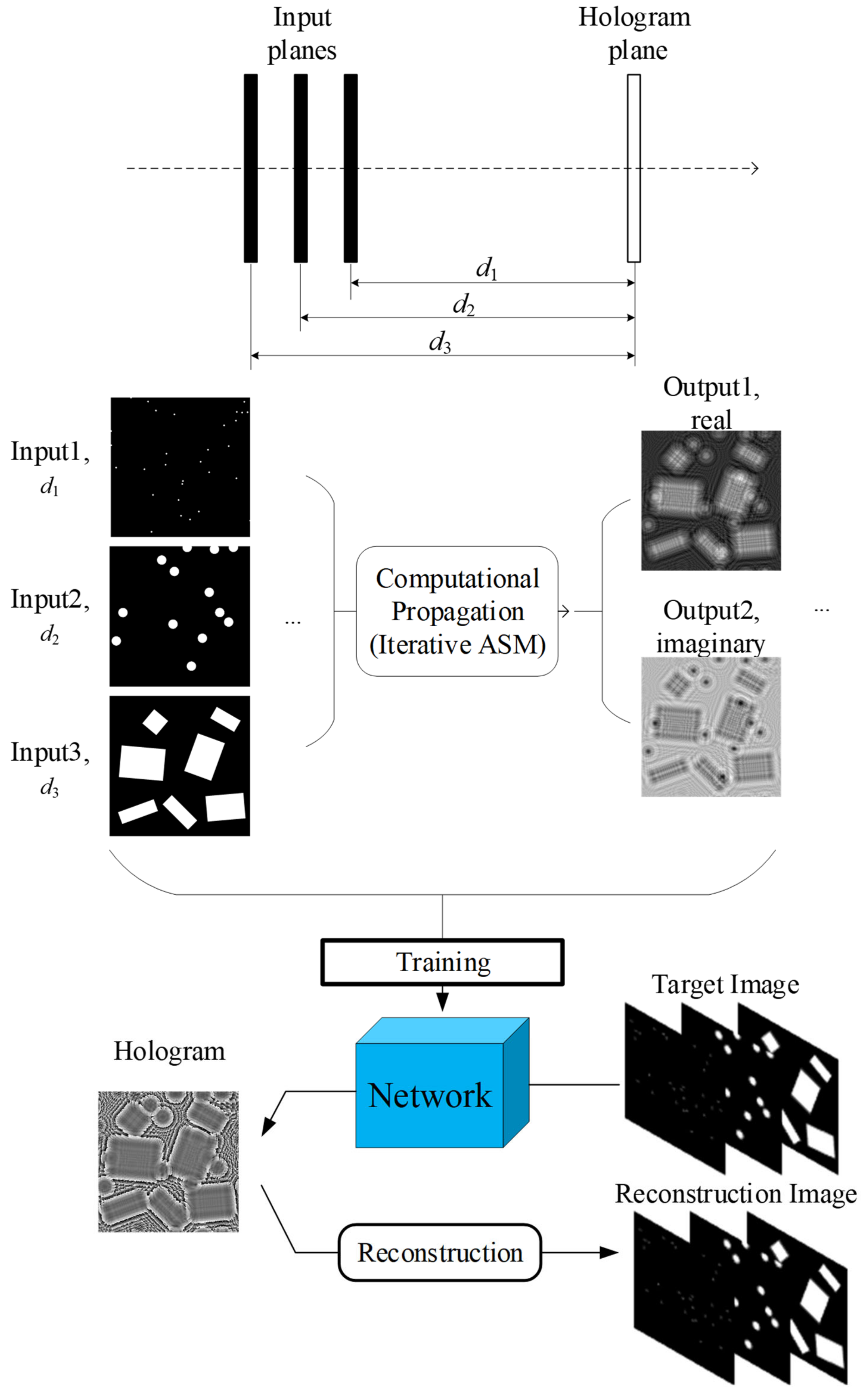
Figure 2 further describes the type of input data and target data provided for network training. The input data are three different images with random dots and rectangular blocks (different size, density and gray scale) and an initial random phase is added to each input image plane. The images are back-propagated to the hologram plane according to each plane from d1 to d3 to obtain a superimposed complex hologram. The plane 1 is closest to the hologram plane at a distance of 98 mm (d1). The plane 3 is farthest from the hologram plane at a distance of 100 mm (d3) and all planes are spaced at 1 mm. The multi-plane iterative ASM is used to generate the complex amplitudes on the hologram plane according to the theory described in Section 2.1 [27,31], which is implemented by MATLAB. The hologram plane pixel spacing and the wavelength of the light source are set to 8 μm and 632.8 nm, respectively. The real and imaginary parts of the hologram are calculated and stored as two different parts of the target data. The size of the input image as well as the hologram is 512 × 512 pixels. In summary, a group of training data contains three sets of images as input data and two groups of superimposed (real and imaginary) holograms as target data. The total training data-set consists of 10,000 groups. A large sample is trained to optimize the loss function and the Adam optimizer [32] is used to find a suitable parameter set for the network.
2.3. The Structure of Network
Figure 3 illustrates the main components of the network structure proposed in the paper. Three images in three different depth planes are provided to the network as input data. The complex hologram calculated by the network possesses the ability to reconstruct each corresponding input image at the corresponding depth plane. The final output of the network is a superimposed complex amplitude in hologram plane divided into two parts, a real part and an imaginary part.
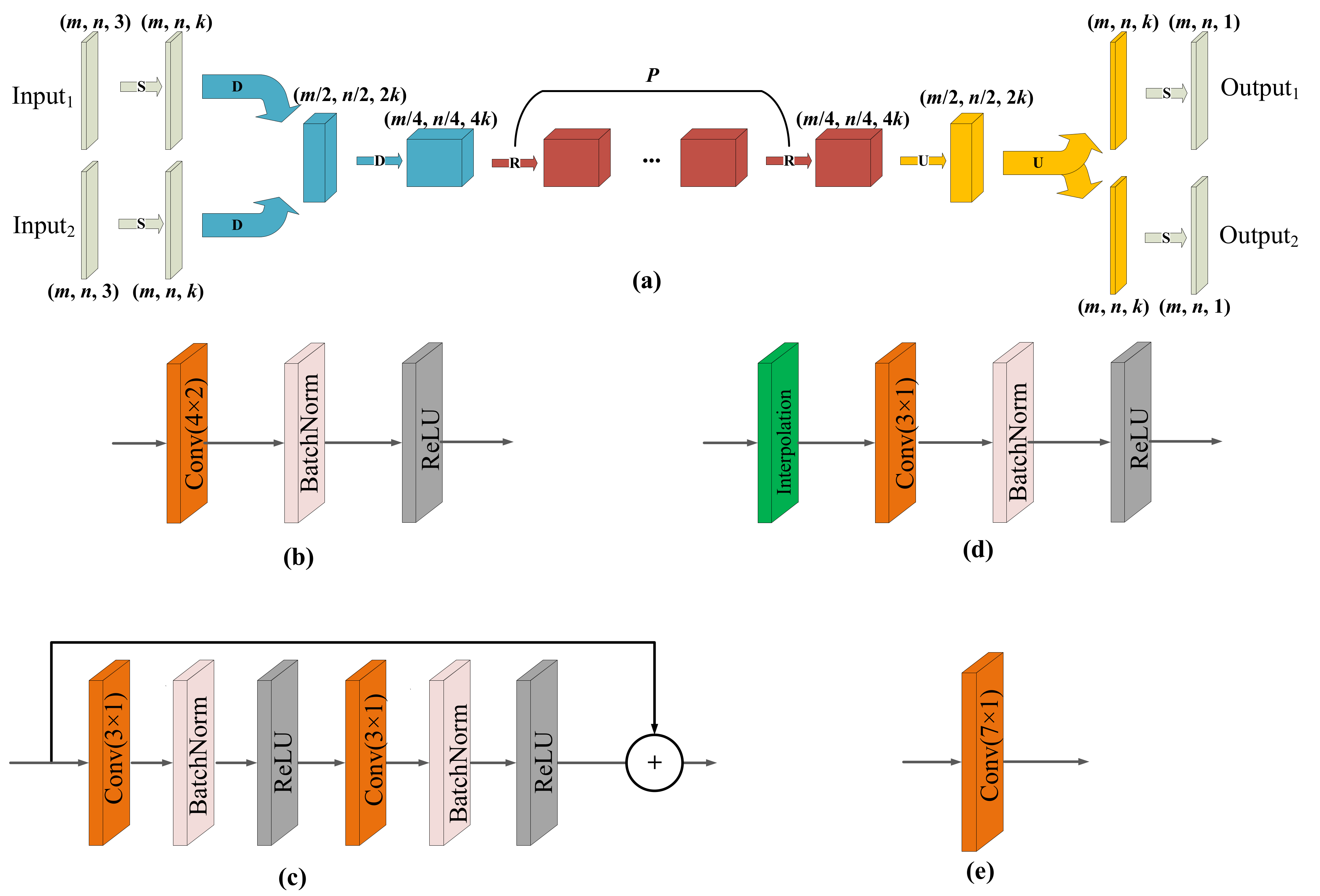
The network structure based on the structure of residual network [33]. It consists of a convolutional layer, a downsampling module, a residual module and an upsampling module, as shown in Figure 3a. Firstly, the network reduces the spatial dimension of the cascaded input image by the downsampling module, while increasing the dimensionality of the channels. After the downsampling module, the processed data immediately pass through some residual blocks. Then, the original spatial dimensions of the image are recovered by the upsampling module. Finally, the real and imaginary parts of the superimposed complex hologram are obtained by the last two output branches. The size of the data after each operation is indicated in brackets and each number in the brackets implies the height, width and number of channels of the respective data matrix. The size of the input data is 512 × 512 (m × n) pixels, the number of convolution filters in the first layer is 128 (k) and the number of residual blocks is 9 (P), as shown in Figure 3a.
The downsampling module, which is part D in Figure 3a, consists of a convolutional layer, a batch normalization layer [34] and a rectified linear unit (ReLU) layer [35], as shown in Figure 3b. The size and step length of the kernel are indicated by the numbers in the convolutional layer frame, which means that the size of the convolutional kernel in the downsampling module is 4 and the step length is 2. The residual module, which is the R part in Figure 3a, consists of two convolutional layers, two batch normalization layers and two rectified linear unit (ReLU) layers, as shown in Figure 3c. The residual module contains a convolutional kernel with size of 3 and step length of 1. After one downsampling module, the image size becomes half of the previous layer and the number of convolution filters becomes twice the previous layer, as shown in Figure 3a. The size of the image and the number of convolution filters do not change before and after the residual module.
In addition, the network has problems such as unavoidable information loss during the transfer of information between the convolutional layers, so a bypass branch [36,37] is added to the residual module to protect the information integrity by transferring the information from the input to the output and also simplifies the difficulty of the learning target. The residual block has good effect on solving the problem of the gradient gradually disappearing as the network goes deeper, which can make the network deeper while preserving the original data information [33] and help the remaining learning of the network. The upsampling module is shown in Figure 3d, which is the U part in Figure 3a. The structure of upsampling module is similar to the downsampling module with an additional interpolation layer to improve the resolution. In the upsampling module, the convolution kernel size is 3 and the step length is 1. The image after an upsampling module becomes twice the size of the previous layer and the number of convolution filters becomes half of the original. Since the image has gone through two downsampling modules, it goes through two more upsampling modules to restore the image to the original input size and output the result.
Finally, a convolution layer (shown in Figure 3e) with a convolution kernel size of 7 and a step length of 1 is added at both the input and output layers that is the S part in Figure 3a, as shown in Figure 3e, to recover the original size of the image and keep it consistent with the input data. After the various parts of the network, the final output is normalized, with a training result of an 8-bit gray-scale phase-only hologram.
2.4. Loss Function
For the loss function, the mean square error (MSE) and the mean absolute error (MAE) are combined to measure the training effect and the algorithm performance. The MSE can be used to represent the degree of image distortion and is used as a loss rating in many images processing related fields with the expression:
The MAE is used to express the sum of the absolute differences between the target and predicted data. It can be measured as the average error size of the predicted data, expressed as:
where M is the total number of data, Ytrue is the target hologram and Ypred is the hologram predicted by the network, which is the output of the network. In training, for outlier data, the middle value will have better robustness than the mean value, so it is necessary to introduce the mean absolute value error based on the mean square error to obtain a more effective and stable output. When training the model, theoretically both of the above equations will reach the minimum when the predicted value is exactly equal to the target value. In all practical training, the ultimate goal is to find the point that minimizes the loss function.
In summary, the complete loss function is the mean square error plus the average absolute error after setting the weight, the weight is empirically set to 0.1 and the expression is:
In fact, no matter how accurate the algorithm is, it is a feasible approximation to the real image and the approximation will always satisfy Loss > 0 in the real world. Therefore, the algorithm is suitable to be used as a loss function for network training and its performance can be quantitatively compared. This loss function is used in both the real and the imaginary parts of complex hologram training process.
3. Experiments and Results Analysis
For the holograms produced by the trained network, it is necessary to verify whether it has the ability to reconstruct different images at the corresponding depths like the reconstruction results of ground-truth CGHs and it is also necessary to compare whether the two results are similar, so as to evaluate whether the network has effectively learned the light propagation process of the iterative ASM. The algorithm is evaluated by actual experimental conditions and the input image size to the network model is set to 512 × 512 pixels and the depth planes are set to three. Considering various scenes, 10,000 groups of samples were generated for training the network model and 5000 samples were generated for testing. The input data are normalized to a range from 0 to 1, which is the basic feasibility criterion that the target intensity distribution must satisfy to help the feature learning of the network.
In the data generation, parameters were chosen to match with the optical reconstruction experiments. That is, the laser wavelength is = 632.8 nm and the pixel spacing of hologram plane is 8 μm. The adjacent depth planes are separated by 1 mm and the number of depth planes is set as three, that is, d1 = 98 mm, d2 = 99 mm and d3 = 100 mm.
The training results of the proposed method are compared with holograms generated by other methods [24,30].
In this paper, the desired network is implemented in PyTorch 1.7.1 with CUDA 11.0 deep learning framework [38,39] using the programming language Python and the network model is trained with an Nvidia GeForce RTX 3090 GPU. The multi-plane iterative ASM was implemented using MATLAB. All methods are tested on an Nvidia GeForce RTX 3090 GPU.
3.1. Numerical Reconstruction
3.1.1. Single Planar Numerical Reconstruction
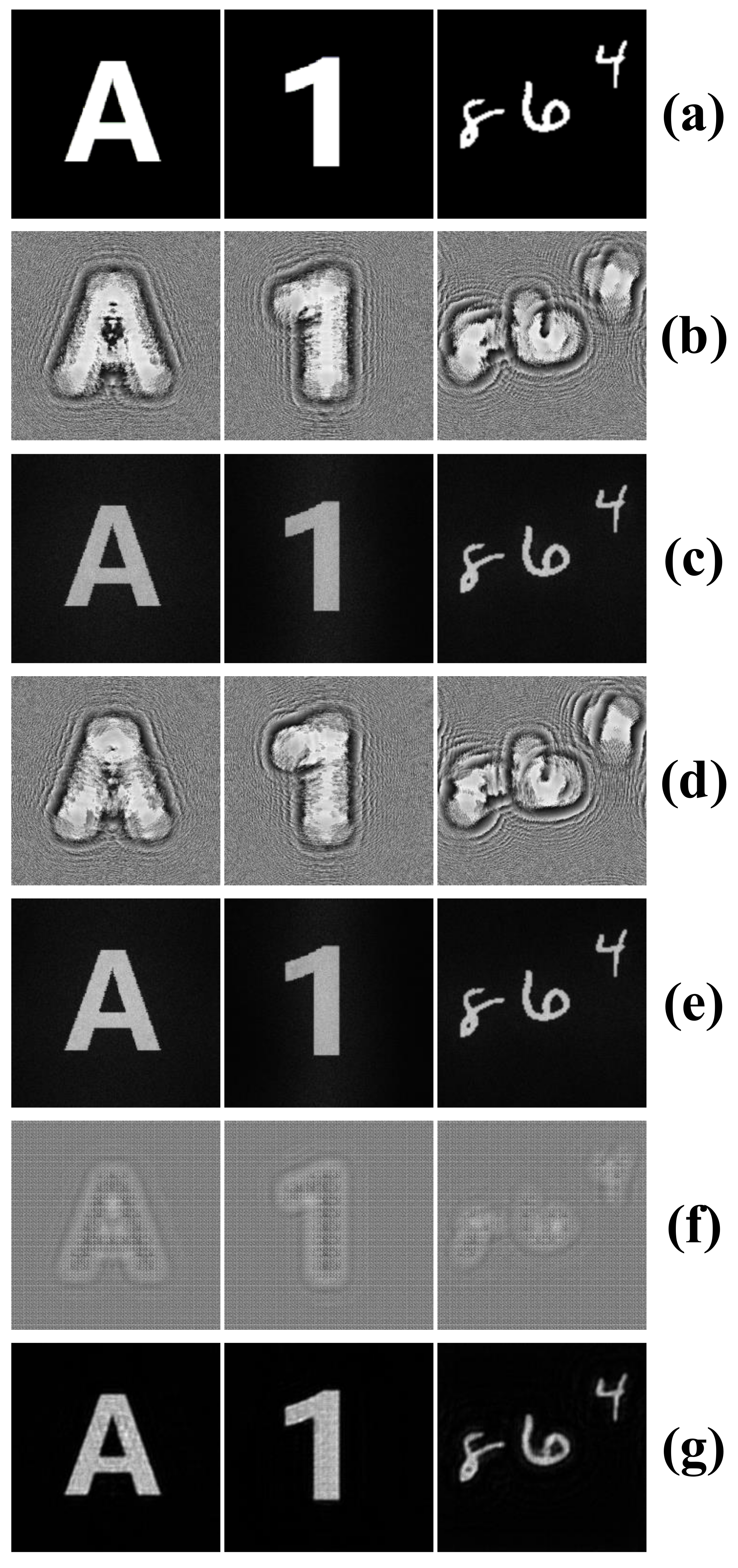
For the single planar numerical reconstruction, the images are used as a test set for a network with one plane of input to obtain the hologram generated by the network. The network-generated images and the reconstruction results are demonstrated by some simple numbers, letters and processed handwritten digit data-sets (random handwritten digit combinations) generated by MATLAB, as shown in Figure 4. The three images shown in Figure 4a are composed of standard letters, standard numbers and handwritten digit data-sets. The hologram in Figure 4b is the result calculated by the trained network; the hologram generated using the network has a high accuracy comparable to existing iterative ASM algorithm even after a large number of iterations. The numerical reconstruction results are shown in Figure 4c and it is clearly seen that for simple images, the output results of the network have a high quality comparable to the existing algorithms after many iterations. The computational holograms based on the iterative ASM are shown in Figure 4d and the numerical reconstruction results are shown in Figure 4e. We also use recent method named holo-encoder [24] to generate and reconstruct the same image and compare the image quality with our work, shown in Figure 4f,g.
To quantitatively validate the results in Figure 4, a test set of 5000 test samples (consisting of the three types of images in Figure 4) is produced for simulating the average accuracy of the results as well as their calculation times. These results are compared with the results of the planar iterative ASM on the same test data-set with 10, 100, and 1000 iterations for each sample. After calculation, the results of each evaluation index for the network and the iterative ASM are shown in the following tables. Table 1 shows the average root mean square error (RMSE), the average coefficient of determination (R2) and the average time required (T in second) for the holograms generated by the two algorithms. Table 2 indicates the evaluation parameters (PSNR and SSIM) of their corresponding reconstructed images.
Table 1 shows the comparison of the results. In the conventional iterative ASM, all the values of evaluation metrics of the images improve with the increase in the number of iterations. The RMSE of the network results is slightly inferior to the results of 1000 iterations of the existing algorithm, but it is still much better than the results of 10 and 100 iterations; the coefficient of determination is comparable with the results of 1000 iterations, but the hologram generation time of the network is in the same level of the time consuming of using iterative ASM with 10 iterations. Meanwhile, the results from the comparison of PSNR and SSIM prove that the network has a significant advantage in the quality of reconstructed images. In summary, for simple planar images, the network generates holograms that are faster than iterative ASM while ensuring high image quality.
Regardless of the algorithm used to generate the computational hologram, its accuracy and speed depend on the image size. For the image size of 512 × 512 pixels, the calculating times of the deep learning-based method and the iterative ASM for calculating a single hologram with a computer with an Intel Core i9-10980XE processor, a clock frequency of 3.0 GHz and a memory size of 32 GB are shown in Table 1. The time consuming for calculating holograms is shorter in the proposed network method, which is about 50 times faster than the iterative ASM at the same quality level; here, we do not consider that the training time of the network is about 50 h. We compare with a recent related study (called as holo-encoder) [24] and calculate the PSNR and RMSE of reconstructed images from the phase hologram generated using a holo-encoder method. The PSNR is 23.3611 and RMSE is 0.0548.
In summary, the simulation results show that the proposed network has the ability to calculate the corresponding hologram with good imaging quality compared with the iterative ASM and the proposed network can perfectly solve the built-in trade-off between imaging quality and calculation speed.
3.1.2. Three-Dimensional Numerical Reconstruction
In order to realize the construction of 3D images, we train the network with three input images located in different depth planes as a test group to obtain the hologram, as shown in Figure 5a. The images “1”, “2”, and “3” are set in order of depth; that is, “1” is closest to the hologram plane and “3” is furthest from the hologram plane (d1 = 98 mm, d2 = 99 mm, d3 = 100 mm). The pixel size of each input image is set as 512 × 512 pixels. Figure 5b,c shows the real and imaginary parts of the generated numerical 3D hologram. The pixel size of the hologram is 512 × 512 pixels. The ground-truth 3D holograms with these three images in the corresponding depths are also generated by using the multi-plane iterative ASM.
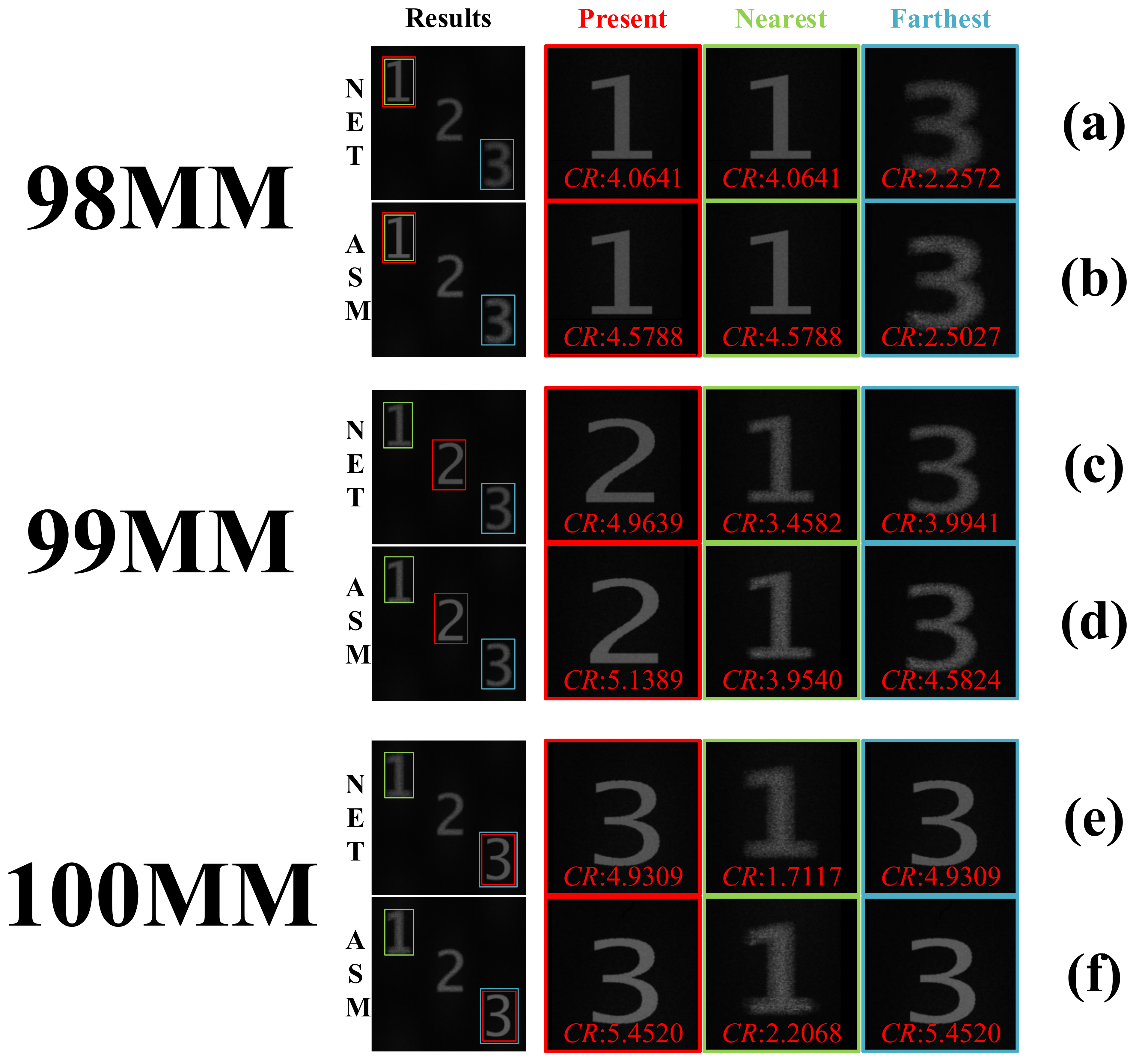
Three images were reconstructed in three different depth planes from d1 to d3. The values of wavelength and pixel spacing of hologram are the same as set in single planar mode. The reconstructed images of the holograms from the multi-plane iterative ASM and the network are shown in Figure 6. In order to more clearly compare the reconstruction results of the images in the corresponding depth planes, the reconstruction results of each image in the corresponding depth planes are enlarged, as shown in the second column of Figure 6a–f. By comparing these reconstruction results, it can be seen that the holograms generated by the network can reconstruct correct image in the corresponding depth plane. The image quality is almost the same as the reconstruction results of the holograms generated by the multi-plane iterative ASM.
In order to evaluate the reconstruction quality of the images and to compare the differences between the focus plane and the unfocused plane in a better way, we introduce contrast ratio (CR) as a parameter, which is calculated by the following formula:
where = || means the grayscale difference between adjacent pixels and means the pixel distribution probability that the grayscale difference between adjacent pixels is . There are two ways to calculate the value of adjacent pixels: 4-adjacent and 8-adjacent. Here, we take 4-adjacent (each pixel only calculates the difference between the top, bottom, left and right directions, the location of the border pixel cannot be taken as the difference value of 0). The results in Figure 6 show that the image quality of the focused plane is significantly better than the unfocused plane and the reconstructed image quality of the network is comparable to iterative ASM.
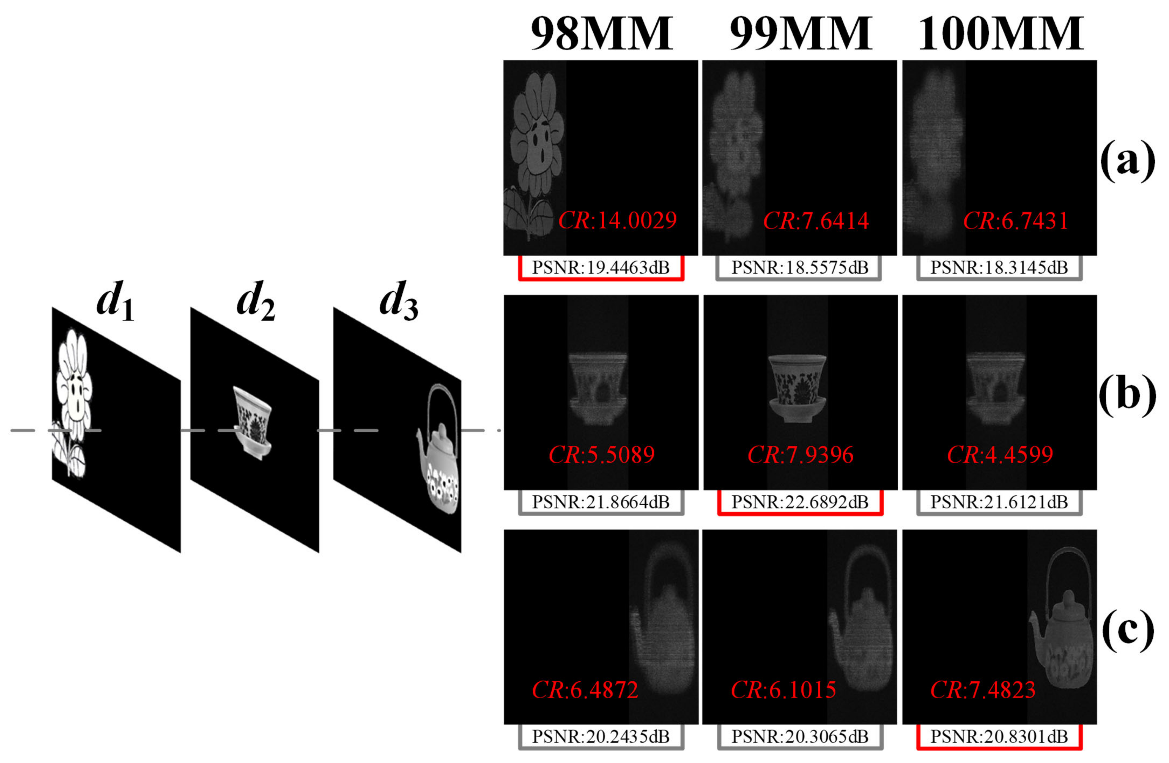
The above numerical reconstruction results demonstrate that the 3D holograms generated by the network have the ability to reconstruct input images at different depths. Next, its ability to recover grayscale images at specific depths is investigated and verified by further numerical simulations. Its performance in complex input cases is verified by inputting complex grayscale images. Figure 7 shows the numerical simulation reconstruction results of the holograms calculated by the network under the new input data configuration. In calculating the hologram, the network receives a set of inputs with three different depth planes and calculates a hologram with multi-depth planes information. Each of these depth planes has a complex image at a different location. Each row in Figure 7 shows the reconstruction results based on the same complex image placed at different depth planes and each column shows the reconstruction results of three different complex images of different depth plane at the same depth plane. For example, Figure 7a shows the complex image’s reconstruction results obtained at three different reconstruction distances from 98 mm to 100 mm which located in the d1 plane. Finally, by calculating the PSNR and CR for all planes, we found that the hologram generated by the network can reconstruct the image clearly in the corresponding depth plane, although the reconstructed image is slightly disturbed by speckle noise. The results also certify that the image quality of the focused plane is significantly better than the unfocused plane.
3.2. Optical Reconstruction
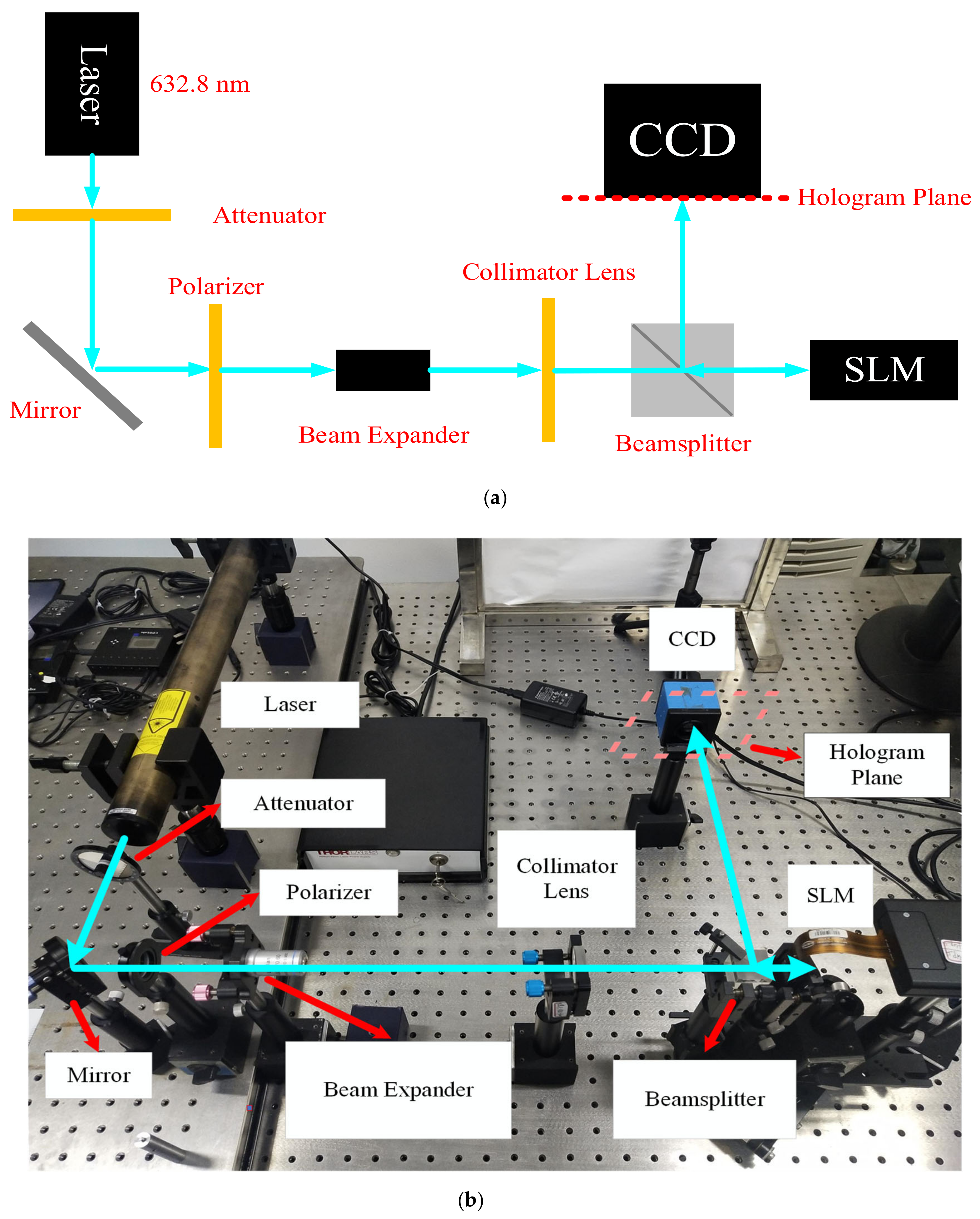
To verify that the network-generated holograms have the ability to be reconstructed optically as effectively as they are numerically, an experimental holographic display device is built, as shown in Figure 8. A phase-only modulation type spatial light modulator (SLM) with pixels of 1920 × 1080 and pixel pitch of 8 μm is used. In addition, the distance between the lenses in the optical imaging system is adjusted to precisely match the corresponding reconstructed positions of the network-generated hologram so that the final hologram plane can reproduce the reconstructed image with the same parameters as the network input data. Optical reconstruction of the network-generated hologram and the hologram generated using the iterative ASM is performed by using the holographic display setup shown in Figure 8.
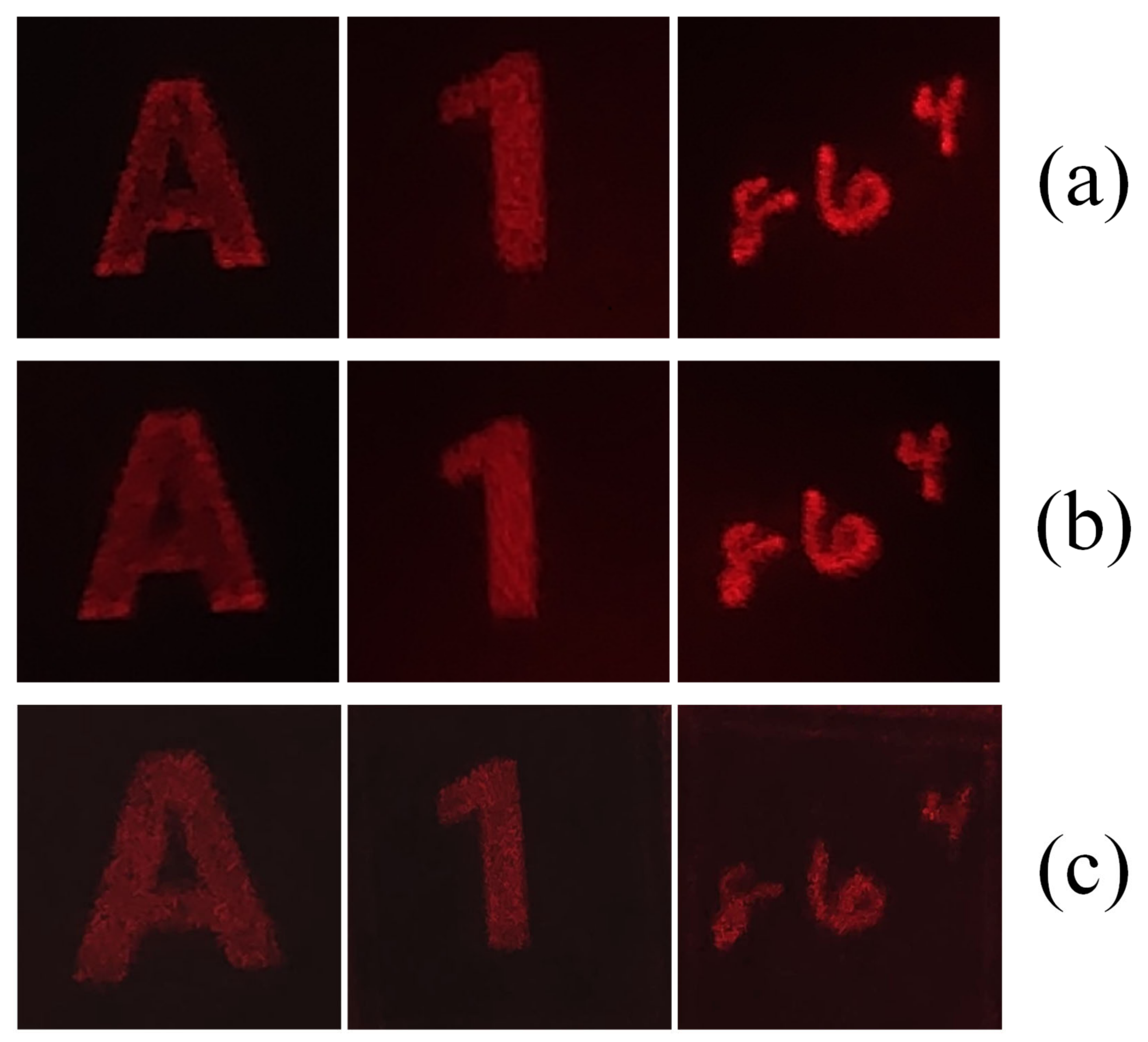
The optical reconstruction results of the holograms generated by the two methods for single plane images shown in Figure 4 are compared, as shown in Figure 9. Optical reconstruction distance is set as 100 mm. The three images in row (a) respectively show the optical reconstruction results of holograms obtained by the ASM for single standard letters, numbers and multiple handwritten numbers, while row (b) shows the optical reconstruction results of holograms obtained by the network for the corresponding images. Moreover, row (c) shows the optical reconstruction results of holograms obtained by holo-encoder for the corresponding images. As can be seen in Figure 9, all methods are able to optically reconstruct the images with similar clarity. The proposed method has convincing optical reconstruction results compared with the traditional iterative ASM and the holo-encoder.
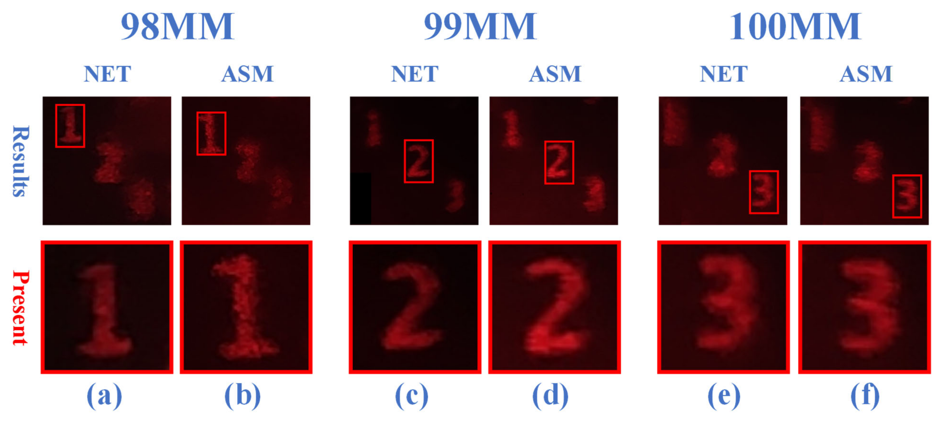
Next, we obtain the optically reconstructed images for each depth plane (from d1 to d3) and compare the results of the multi depths images. The distances of d1, d2, and d3 are 98 mm to 100 mm and the interval of each plane is 1 mm; the iterative ASM results for 1000 iterations and the test results for the network are shown in Figure 10. The columns (a), (c) and (e) in the figure show the optically reconstructed images of the network and their corresponding magnified images of the focused plane information; the columns (b), (d) and (f) show the optically reconstructed images of the iterative ASM and their corresponding magnified images of the focused plane information. By comparing the results in the first row of Figure 10, it can be seen that the holograms generated by the network also have the ability to reconstruct clear images in the corresponding depth planes, as the holograms generated by the conventional iterative ASM. Furthermore, the results in the second row of Figure 10 verify that the holograms generated by both methods can obtain similarly sharp optical reconstruction results in the depth plane of focus. Thus, it is experimentally confirmed that the holograms generated by the network can be optically reconstructed and obtain similar results as those generated by the iterative ASM.
3.3. Generalizability Test
A network model is considered generalizable when it does not overfit the data-set in which it is trained and is able to calculate accurate results that are not from the data-set. By this definition, if the model trained with random scatters in this paper can calculate non-scattered and equally high-quality holograms and reconstruction results, it can show that the network in this paper is generalizable.
Generalizability is a very valuable feature of current neural network algorithms, especially for real-world experimental needs, where each class of images has its own unique and distinctive characteristics. Training a specific model for each class of samples is obviously inefficient and time-consuming.
To evaluate the generalizability of the network, we generate and compare the accuracy of the model tested on different types of data. In this paper, numbers, letters and complex images mentioned in Section 3.1.1 and Section 3.1.2 are used as test sets. The results for simple images are shown in Table 1 and Table 2, while the performance evaluation of reconstruction results for 5000 test samples with data types of complex images (such as the effective multi depth planes images in Figure 7) is shown in Table 3. When testing the model on different type of test data-sets, the accuracy of the network is slightly reduced, especially for the case of complex images due to the presence of numerous noise and detail features, which makes both SSIM and PSNR decrease compared to simple images. However, the accuracy is still very advantageous compared to conventional algorithms, which further validates the generalization of the proposed network and perfectly illustrates the generalization of the mapping that the network learned from the random dots and rectangular blocks (different size, density and gray scale) data-set for generating high-quality holograms of completely different nature. The holograms generated by the network as well as the reconstructed images seem almost the same in image detail with the results obtained with iterative ASM, the speed of the proposed network has a considerable advantage over iterative algorithms and it has potential applications in special situation requiring real-time responses.
Moreover, for some specific applications, it is possible to purposefully select suitable specific data types as training sets and adjust the loss function to output specific results, thus allowing the network to have performance improvements for specific applications at the cost of generalizability.
4. Discussion
The problems to be further investigated in this paper focus on the reconstruction of more complex holograms and the number of depth planes. Since the neural network is more focused on solving the same kind of problems, the results may deviate more when the input images are somewhat different from the training set. The results in scenarios such as image occlusion or scatter reduction are some of the problems that have not yet been taken into account. However, with the development of network structure and training strategy as well as the deepening of the degree of knowledge between deep learning and optical problems, these problems are expected to be solved in the future. As for the depth plane problem, currently the experimental workstation GPU is almost completely occupied when the depth plane is three, but it is possible to make the network learn more depth planes by adjusting the network structure and using hardware with more computational power. As a result, the network can learn the rules of wavefront propagation in the future, achieving the ability to generate multi-depth holograms more efficiently than traditional iterative methods. Even more realistic reconstructed objects can be achieved if enough depth planes are learned, which will have more advantages in the future.
5. Conclusions
This paper presents a method for computing 3D phase-type holograms based on deep learning, which can be used to solve the problem of generating accurate planar or 3D holograms faster compared to traditional iterative ASM. An effective network training strategy is developed while setting up a network with a structure consisting of a downsampling module, a residual module, and an upsampling module. Instead of using a training data-set of random dots, the network combines various types of data-sets to optimize the reconstructed images simultaneously. In addition, intermediate variables are used as target data in the training process to make the training more efficient and to improve the robustness by adding random phases to the input data. The network is able to reconstruct high-quality images in the corresponding depth plane with some generalization through numerical simulations and optical reconstruction. However, this paper is currently limited to discussing the generation of equally spaced holograms with at most three planes. The problems of hologram occultation ratio, the effect of scattering on imaging quality during photoelectric reconstruction (loss of image details) and training holograms of more depth planes have not been studied. However, with the development of the network structure and further research on the network parameters, all of these problems are expected to be solved in the future.
Author Contributions
J.H.: Writing original draft, methodology, validation, visualization and writing— review and editing; X.W.: Supervision and visualization; C.Z.: Data acquisition and software; H.Z.: Writing— review and editing, investigation and supervision. All authors have read and agreed to the published version of the manuscript.
Funding
This work was supported by the National Natural Science Foundation of China (Grant No. 61875115), Key Laboratory of Advanced Display and System Application, Chinese Ministry of Education (Grant No. P201610).
Institutional Review Board Statement
Not applicable.
Informed Consent Statement
Not applicable.
Data Availability Statement
The data presented in this study are available on reasonable request from the corresponding author.
Conflicts of Interest
The authors declare no conflict of interest.
References
- Park, J.H. Recent progress in computer-generated holography for three-dimensional scenes. J. Inf. Disp. 2016, 18, 1–12. [Google Scholar] [CrossRef] [Green Version]
- Matsushima, K. Introduction to Computer Holography; Springer: Berlin/Heidelberg, Germany, 2020. [Google Scholar]
- Lohmann, A.W.; Paris, D.P. Binary Fraunhofer Holograms, Generated by Computer. Appl. Opt. 1967, 6, 1739–1748. [Google Scholar] [CrossRef] [PubMed]
- Guo, C.; Shen, C.; Li, Q.; Tan, J.B.; Liu, S.T.; Kan, X.C.; Liu, Z.J. A fast-converging iterative method based on weighted feedback for multi-distance phase retrieval. Sci. Rep. 2018, 8, 6436. [Google Scholar] [CrossRef]
- Endo, Y.; Shimobaba, T.; Kakue, T.; Ito, T. GPU-accelerated compressive holography. Opt. Express 2016, 24, 8437–8445. [Google Scholar] [CrossRef]
- Anand, V.; Katkus, T.; Linklater, D.P.; Ivanova, E.P.; Juodkazis, S. Lensless Three-Dimensional Quantitative Phase Imaging Using Phase Retrieval Algorithm. J. Imaging 2020, 6, 99. [Google Scholar] [CrossRef]
- Gerchberg, R.W.; Saxton, W.O. A practical algorithm for the determination of phase from image and diffraction plane pictures. Optik 1971, 35, 237–250. [Google Scholar]
- Makowski, M.; Sypek, M.; Kolodziejczyk, A.; Mikuła, G.; Suszek, J. Iterative design of multiplane holograms: Experiments and applications. Opt. Eng. 2007, 46, 045802. [Google Scholar] [CrossRef]
- Bengtsson, J. Kinoform design with an optimal-rotation-angle method. Appl. Opt. 1994, 33, 6879–6884. [Google Scholar] [CrossRef]
- Pang, H.; Wang, J.Z.; Zhang, M.; Cao, A.X.; Shi, L.F.; Deng, Q.L. Non-iterative phase-only Fourier hologram generation with high image quality. Opt. Express 2017, 25, 14323–14333. [Google Scholar] [CrossRef]
- Sui, X.M.; He, Z.H.; Jin, G.F.; Chu, D.P.; Cao, L.C. Band-limited double-phase method for enhancing image sharpness in complex modulated computer-generated holograms. Opt. Express 2020, 29, 2597–2612. [Google Scholar] [CrossRef]
- Maimone, A.; Georgiou, A.; Kollin, J.S. Holographic near-eye displays for virtual and augmented reality. ACM Trans. Graph. 2017, 36, 1–16. [Google Scholar] [CrossRef]
- Cun, L.Y.; Bengio, Y.; Hinton, G. Deep learning. Nature 2015, 521, 436–444. [Google Scholar]
- Kiarashinejad, Y.; Abdollahramezani, S.; Adibi, A. Deep learning approach based on dimensionality reduction for designing electromagnetic nanostructures. NPJ Comput. Mater. 2020, 6, 12. [Google Scholar] [CrossRef]
- Kiarashinejad, Y.; Zandehshahvar, M.; Abdollahramezani, S.; Hemmatyar, O.; Pourabolghasem, R.; Adibi, A. Knowledge Discovery In Nanophotonics Using Geometric Deep Learning. Adv. Intell. Syst. 2019, 2, 1900132. [Google Scholar] [CrossRef] [Green Version]
- Rivenson, Y.; Zhang, Y.; Günaydın, H.; Teng, D.; Ozcan, A. Phase recovery and holographic image reconstruction using deep learning in neural networks. Light Sci. Appl. 2018, 7, 17141. [Google Scholar] [CrossRef]
- Barbastathis, G.; Ozcan, A.; Situ, G.H. On the use of deep learning for computational imaging. Optica 2019, 6, 921–943. [Google Scholar] [CrossRef]
- Meng, L.; Wang, H.; Li, G.; Zheng, S.; Situ, G.H. Learning-based lensless imaging through optically thick scattering media. Adv. Photonics 2019, 1, 036002. [Google Scholar]
- Shi, L.; Li, B.C.; Kim, C.; Kellnhofer, P.; Matusik, W. Towards real-time photorealistic 3D holography with deep neural networks. Nature 2021, 591, 234–239. [Google Scholar] [CrossRef]
- Kang, J.W.; Lee, J.E.; Lee, Y.H.; Kim, D.W.; Seo, Y.H. Interference Pattern Generation by using Deep Learning based on GAN. In ITC CSCC; IEEE: JeJu, Korea, 2019; pp. 1–2. [Google Scholar]
- Horisaki, R.; Takagi, R.; Tanida, J. Deep-learning-generated holography. Appl. Opt. 2018, 57, 3859–3863. [Google Scholar] [CrossRef]
- Lee, J.; Jeong, J.; Cho, J.; Yoo, D.; Lee, B.; Lee, B. Deep neural network for multi-depth hologram generation and its training strategy. Opt. Express 2020, 28, 27137–27154. [Google Scholar] [CrossRef]
- Lee, J.; Jeong, J.; Cho, J.; Yoo, D.; Lee, B. Complex hologram generation of multi-depth images using deep neural network. In 3D Image Acquisition and Display: Technology, Perception and Applications; Optical Society of America: Washington, DC, USA, 2020. [Google Scholar]
- Wu, J.C.; Liu, K.X.; Sui, X.M.; Cao, L.C. High-speed computer-generated holography using autoencoder-based deep neural network. Opt. Lett. 2021, 46, 2908–2911. [Google Scholar] [CrossRef]
- Goodman, J.W.; Lawrence, R.W. Digital Image Formation from Electronically Detected Holograms. Appl. Phys. Lett. 1967, 11, 77–79. [Google Scholar] [CrossRef]
- Goodman, J.W. Introduction to Fourier Optics, 3rd ed.; Roberts and Company Publishers: New York, NY, USA, 2004. [Google Scholar]
- Zhou, P.C.; Bi, Y.; Sun, M.; Wang, H.; Li, F.; Qi, Y. Image quality enhancement and computation acceleration of 3D holographic display using a symmetrical 3D GS algorithm. Appl. Opt. 2014, 53, 209–213. [Google Scholar] [CrossRef]
- Kyoji, M.; Tomoyoshi, S. Band-limited angular spectrum method for numerical simulation of free-space propagation in far and near fields. Opt. Express 2009, 17, 19662–19673. [Google Scholar]
- Matsushima, K.; Schimmel, H.; Wyrowski, F. Fast calculation method for optical diffraction on tilted planes by use of the angular spectrum of plane waves. J. Opt. Soc. Am. A Opt. Image Sci. Vis. 2003, 20, 1755–1762. [Google Scholar] [CrossRef]
- Fan, S.; Zhang, Y.P.; Wang, F.; Gao, Y.L.; Qian, X.F.; Zhang, Y.A.; Xu, W.; Cao, L.C. Gerchberg-Saxton algorithm and angular-spectrum layer-oriented method for true color three-dimensional display. Acta. Phys. Sin. CH Ed. 2018, 67, 094203. [Google Scholar]
- Yan, K.T.; Yu, Y.Y.; Sun, T.; Asundi, A.; Qian, K.M. Wrapped phase denoising using convolutional neural networks. Opt. Lasers Eng. 2020, 128, 105999. [Google Scholar] [CrossRef]
- Kingma, D.; Ba, J. Adam: A Method for Stochastic Optimization. International Conference for Learning Representations; Machine Learning: San Diego, CA, USA, 2015. [Google Scholar]
- He, K.; Zhang, X.; Ren, S.; Sun, J. Deep Residual Learning for Image Recognition. In IEEE Conference on Computer Vision & Pattern Recognition; IEEE Computer Society: Washington, DC, USA, 2016. [Google Scholar]
- Ioffe, S.; Szegedy, C. Batch normalization: Accelerating deep network training by reducing internal covariate shift. In Proceedings of the International Conference on Machine Learning, Lille, France, 1 January 2015; pp. 448–456. [Google Scholar]
- Nair, V.; Hinton, G.E. Rectified Linear Units Improve Restricted Boltzmann Machines Vinod Nair. In Proceedings of the 27th International Conference on Machine Learning, Haifa, Israel, 21–24 June 2010. [Google Scholar]
- Goodfellow, I.; Bengio, Y.; Courville, A. Deep Learning; MIT Press: Cambridge, MA, USA, 2016. [Google Scholar]
- Eybposh, M.H.; Ebrahim-Abadi, M.H.; Jalilpour-Monesi, M.; Saboksayr, S.S. Segmentation and Classification of Cine-MR Images Using Fully Convolutional Networks and Handcrafted Features. arXiv 2017, arXiv:1709.02565. [Google Scholar]
- PyTorch Tutorials. Available online: https://pytorch.org/tutorials/ (accessed on 30 May 2021).
- Subramanian, V. Deep Learning with PyTorch: A Practical Approach to Building Neural Network Models Using PyTorch; Packt Publishing: Birmingham, UK, 2018. [Google Scholar]
Figure 1.
The propagation diagram of the 3D iterative ASM.

Figure 2.
Diagram of neural network for hologram generation.

Figure 3.
Network structure and specific components of each module. (a) is the overall structure of the network, consisting of (b) the downsampling module (D-part), (c) the residual module (R-part), (d) the upsampling module (U-part) and (e) the convolution layer at the input and output layers. The data dimensions in each module are expressed as (height, width, channel). A pair of numbers in the convolution layer, e.g., Conv (7, 1) indicates the size and step of the convolution kernel.

Figure 4.
Hologram generation and reconstruction of planar images. Row (a) is the target image, row (b) is holograms generated by network, row (c) is the reconstruction result of network, row (d) is holograms generated by iterative ASM, row (e) is the reconstruction result of iterative ASM, row (f) is holograms generated by holo-encoder, and row (g) is the reconstruction result of holo-encoder.

Figure 5.
Diagram of generating holograms from input images using deep learning. (a) trained network, (b) real part of hologram, (c) imaginary part of hologram.
Figure 5.
Diagram of generating holograms from input images using deep learning. (a) trained network, (b) real part of hologram, (c) imaginary part of hologram.

Figure 6.
Comparison of numerical reconstruction results of multi-plane iterative ASM and network. Rows (a,c,e) are the reconstructed image results of the network and the magnified images corresponding to the details; rows (b,d,f) are the reconstructed image results of the multi-plane iterative ASM and the magnified details images. Three columns on the right of Figure 6 are all magnification results corresponding to the individual digits in the reconstructed image.

Figure 7.
Testing the reconstruction of hologram images after inputting complex images. Each of the three input planes has a complex image at a different location, where the depth plane d1 is closest to the hologram plane and the numerical reconstruction results are shown in rows (a,b,c) when the focusing plane is located in the depth planes d1, d2 and d3, respectively. The PSNR and the CR in the corresponding focused depth plane are shown in the corresponding images.

Figure 8.
Schematic diagram of the optical path used for optical reconstruction and the actual optical device. (a) shows the schematic diagram of the optical path used for optical reconstruction; (b) shows the optical path system built with the actual experimental setup for optical reconstruction.
Figure 8.
Schematic diagram of the optical path used for optical reconstruction and the actual optical device. (a) shows the schematic diagram of the optical path used for optical reconstruction; (b) shows the optical path system built with the actual experimental setup for optical reconstruction.

Figure 9.
Optical reconstruction results of single-plane simple images. Three images in row (a) are the reconstructed images of the results obtained by the iterative ASM, row (b) is the reconstructed image of the results obtained by the network for the corresponding image, and row (c) is the reconstructed image of the results obtained by holo-encoder for the corresponding image.

Figure 10.
Comparison of optical reconstruction results of iterative ASM and network. Columns (a,c,e) are the optically reconstructed images of the network and their corresponding magnified images of the focused plane information; columns (b,d,f) are the optically reconstructed images of the iterative ASM and their corresponding magnified images of the focused plane information.


Table 1.
Performance evaluation of different methods based on simple images.
| ASM (10) | ASM (100) | ASM (1000) | Proposed Network | |
|---|---|---|---|---|
| RMSE | 0.3393 | 0.0996 | 0.0440 | 0.0492 |
| R2 | 0.8637 | 0.9625 | 0.9910 | 0.9893 |
| T (s) | 0.1065 | 0.9326 | 9.1442 | 0.1889 |
Table 2.
Performance evaluation of reconstruction results of different methods.
| ASM (10) | ASM (100) | ASM (1000) | Proposed Network | |
|---|---|---|---|---|
| PSNR | 7.5191 | 18.1646 | 25.2519 | 24.2920 |
| SSIM | 0.6591 | 0.7980 | 0.8306 | 0.8091 |
Table 3.
Performance evaluation of reconstruction results based on complex images.
| ASM (10) | ASM (100) | ASM (1000) | Network | |
|---|---|---|---|---|
| RMSE | 0.3134 | 0.1239 | 0.0506 | 0.0572 |
| R2 | 0.6081 | 0.7719 | 0.8737 | 0.8413 |
| PSNR | 8.2088 | 16.2694 | 24.0398 | 22.9885 |
| SSIM | 0.5942 | 0.6527 | 0.7209 | 0.6854 |
Publisher’s Note: MDPI stays neutral with regard to jurisdictional claims in published maps and institutional affiliations. |
© 2021 by the authors. Licensee MDPI, Basel, Switzerland. This article is an open access article distributed under the terms and conditions of the Creative Commons Attribution (CC BY) license (https://creativecommons.org/licenses/by/4.0/).
Share and Cite
MDPI and ACS Style
Zheng, H.; Hu, J.; Zhou, C.; Wang, X. Computing 3D Phase-Type Holograms Based on Deep Learning Method. Photonics 2021, 8, 280. https://0-doi-org.brum.beds.ac.uk/10.3390/photonics8070280
AMA Style
Zheng H, Hu J, Zhou C, Wang X. Computing 3D Phase-Type Holograms Based on Deep Learning Method. Photonics. 2021; 8(7):280. https://0-doi-org.brum.beds.ac.uk/10.3390/photonics8070280
Chicago/Turabian StyleZheng, Huadong, Jianbin Hu, Chaojun Zhou, and Xiaoxi Wang. 2021. "Computing 3D Phase-Type Holograms Based on Deep Learning Method" Photonics 8, no. 7: 280. https://0-doi-org.brum.beds.ac.uk/10.3390/photonics8070280
Note that from the first issue of 2016, this journal uses article numbers instead of page numbers. See further details here.