Article

Formation of Inverse Energy Flux in the Case of Diffraction of Linearly Polarized Radiation by Conventional and Generalized Spiral Phase Plates

by
Andrey V. Ustinov
1,
Svetlana N. Khonina
1,2 and
Alexey P. Porfirev
1,*
1
Image Processing Systems Institute—Branch of the Federal Scientific Research Centre, “Crystallography and Photonics” of Russian Academy of Sciences, 443001 Samara, Russia
2
Department of Technical Cybernetics, Samara National Research University, 443086 Samara, Russia
*
Author to whom correspondence should be addressed.
Submission received: 21 June 2021 / Revised: 13 July 2021 / Accepted: 15 July 2021 / Published: 16 July 2021
(This article belongs to the Special Issue Polarized Light and Optical Systems)

Abstract

:
Recently, there has been increased interest in the shaping of light fields with an inverse energy flux to guide optically trapped nano- and microparticles towards a radiation source. To generate inverse energy flux, non-uniformly polarized laser beams, especially higher-order cylindrical vector beams, are widely used. Here, we demonstrate the use of conventional and so-called generalized spiral phase plates for the formation of light fields with an inverse energy flux when they are illuminated with linearly polarized radiation. We present an analytical and numerical study of the longitudinal and transverse components of the Poynting vector. The conditions for maximizing the negative value of the real part of the longitudinal component of the Poynting vector are obtained.

Graphical Abstract

1. Introduction

The ability to shape light fields with the desired complex structure, so-called structured laser beams, plays an important role in the field of laser manipulation for implementing optical tweezers with advanced functionality. Conventional optical tweezers are unique tools that use a strongly focused Gaussian laser beam for the trapping and three-dimensional confinement of nano- and microparticles. Structured optical tweezers, also called holographic optical tweezers (HOT), provide more possibilities for laser manipulation due to the possibility of controlling the local distribution of the optical forces acting on the particles located in such a light field. For example, trapped particles can be guided along with the desired two- or three-dimensional trajectory or rotated with a desired frequency depending on the parameters of the used HOT. Recently, laser beams with an inverse energy flux have attracted researchers’ attention. Such light fields allow the optically trapped particle to be pulled towards the radiation source, i.e., in the direction opposite to field propagation. Researchers have studied the formation of such advanced optical tweezers using light fields with phase or polarization singularities. Currently, the most popular element for generating light fields with phase singularities is probably the conventional spiral phase plate (SPP) [1], an optical element with a complex transmission function exp(imφ), where φ is the polar angle and m is the topological charge of the formed vortex beam. The wide popularity and spread of this element have led to a growth of studies on its various modifications and generalizations to obtain new effective elements for forming light fields with phase singularities with new properties. In particular, if conventional SPPs with an integer value of m form vortex beams with an annular intensity distribution [2,3], then SPPs with a fractional value of m [4] allow more complex intensity distributions [5] and can be used for additional information coding [6]. A power-exponent phase plate (PEPP) [7,8] with the transmission function described as exp[im(φ/2π)s], where m and s are arbitrary numbers and φ is an azimuthal angle, can be used for shaping a spiral intensity distribution. In 2020, we showed that a generalized spiral phase plate (GSPP) [9,10] with the transmission function exp[ig(φ)], where g(φ) is an arbitrary smooth monotonic function, always forms a spiral intensity distribution with a phase singularity point in the focal plane of a lens. Variations in the phase function g(φ) affect the size and the twisting degree of the generated light spiral, thereby determining the phase gradient along the light curve, which is an important light-field characteristic for laser manipulation [11,12,13]. The transverse energy flow density, which is proportional to the product of the field intensity and phase gradient [14,15], allows guiding the trapped particle in a certain direction. However, the longitudinal distribution of the energy flow density is a key for realizing light fields with an inverse energy flux. The inverse energy flux phenomena [16,17,18,19,20] is related to “tractor beams” [21,22,23] in optical trapping and manipulation and to the detection of “invisibility cloaks” [24]. It should be noted that just one inverse energy flux does not guarantee the existence of the pulling optical force—the optical force can be negative due to the negative Poynting vector component, but its effect is often blocked by the gradient-phase force [25,26,27,28].
Earlier, the possibility of forming an inverse energy flux in the focal region for cylindrical vector beams (CVBs) of various orders was investigated, as was a linearly polarized beam with a cosine amplitude distribution [17,18]. Despite the existence of many methods for forming CVBs, linearly polarized laser sources remain the most readily available, affordable, and widespread. Therefore, in this work, we investigate the possibility of forming inverse energy flux in the focal region for a linearly polarized beam under diffraction by both conventional and generalized SPPs. Due to the generation of non-annular light distributions, GSPPs provide more opportunities to control the distribution of optical forces acting on the trapped particle. In particular cases, we carry out analytical and numerical studies of both the longitudinal and transverse components of the Poynting vector, including both the real and the imaginary part. Recently, the imaginary part of this component has attracted attention from researchers [29,30,31,32], since it was shown to contribute to the transverse force acting on optically trapped Mie particles [29,30].

2. Methods

Consider the focused electromagnetic field in the focal region in the framework of the Debye theory [33,34,35]:
[ E ( r , γ , z ) H ( r , γ , z ) ] = i f λ 0 θ max 0 2 π T ( θ ) F ( θ , φ ) [ Q E ( θ , φ ) Q H ( θ , φ ) ] exp { i k [ r sin θ cos ( φ γ ) + z cos θ ] } sin θ d θ d φ ,
where (r, γ, z) are the cylindrical coordinates in the focal region, (θ, φ) are the spherical angular coordinates of the focusing system’s output pupil, θmax is the maximum value of the azimuthal angle related to the system’s numerical aperture, F(θ, φ) is the complex amplitude of the input field, T(θ) is the pupil’s apodization function ( T ( θ ) = cos θ for aplanatic systems), k = 2π/λ is the wavenumber, λ is the wavelength, f is the focal length, and (cx(θ, φ), cy(θ, φ))T is the vector of polarization coefficients of the input field,
Q E ( θ , φ ) = [ A ( θ , φ ) C ( θ , φ ) C ( θ , φ ) B ( θ , φ ) D ( θ , φ ) E ( θ , φ ) ] ( c x ( θ , φ ) c y ( θ , φ ) ) , Q H ( θ , φ ) = [ C ( θ , φ ) A ( θ , φ ) B ( θ , φ ) C ( θ , φ ) E ( θ , φ ) D ( θ , φ ) ] ( c x ( θ , φ ) c y ( θ , φ ) ) ,
with
A ( θ , φ ) = 1 cos 2 φ ( 1 cos θ ) , B ( θ , φ ) = 1 sin 2 φ ( 1 cos θ ) , C ( θ , φ ) = sin φ cos φ ( 1 cos θ ) , D ( θ , φ ) = cos φ sin θ , E ( θ , φ ) = sin φ sin θ .
The complex Poynting vector [29,30,31,32] is proportional to the following expression:
P E * × H .
The real part of expression (4) is a standard Poynting vector, and the imaginary part is interesting, as it relates to exciting non-standard forces arising at the interaction between electric- and magnetic-induced dipoles [29].
In this work, we focus on the longitudinal component of the Poynting vector, which is proportional to the following expression [36]:
P z E x * H y E y * H x .
Note that Re[Pz] is the most important for our research, since it allows us to determine the areas of reverse energy flow. In addition, the azimuthal component of the Poynting vector Re[Pγ], which is related to the longitudinal component of the angular momentum, is also interesting [37,38]:
j z Re [ r × P ] z = Re [ x P y y P x ] = r Re [ P y cos γ P x sin γ ] = r Re [ P γ ] .
Further, we consider the relative magnitudes of negative and positive values, so constants and common factors can be ignored. To obtain explicit analytical expressions, consider an input field with a superimposed narrow annular aperture with a central angle θ0 and width Δ [39,40]:
F ( θ , φ ) = F ( θ 0 , φ ) = S ( θ 0 ) F 0 ( φ )
where F0(φ) is an arbitrary function and
S ( θ 0 ) = { 1 , | θ θ 0 | Δ / 2 , 0 , e l s e .
In this case, the field components in Equation (4) are calculated in the focal plane (z = 0) by the following formulas:
( E x ( r , γ , z ) E y ( r , γ , z ) E z ( r , γ , z ) ) t ( θ 0 , z ) 0 2 π F ( θ 0 , φ ) [ A ( θ 0 , φ ) C ( θ 0 , φ ) C ( θ 0 , φ ) B ( θ 0 , φ ) D ( θ 0 , φ ) E ( θ 0 , φ ) ] ( c x ( θ 0 , φ ) c y ( θ 0 , φ ) ) G ( r , ( φ γ ) ) d φ , ( H x ( r , γ , z ) H y ( r , γ , z ) H z ( r , γ , z ) ) t ( θ 0 , z ) 0 2 π F ( θ 0 , φ ) [ C ( θ 0 , φ ) A ( θ 0 , φ ) B ( θ 0 , φ ) C ( θ 0 , φ ) E ( θ 0 , φ ) D ( θ 0 , φ ) ] ( c x ( θ 0 , φ ) c y ( θ 0 , φ ) ) G ( r , ( φ γ ) ) d φ ,
where t ( θ 0 , z ) = i exp ( i k z cos θ 0 ) cos θ 0 sin θ 0 Δ f / λ , G ( r , φ ) = exp ( i k r sin θ 0 cos φ ) .

3. Results

As an input field F0, φ), consider a plane x-linearly polarized laser beam with the polarization vector (cx0, φ), cy0, φ))T = (1, 0)T, passed through a GSPP [9,10]:
F 0 ( φ ) = exp [ i g ( φ ) ] ,
where g(φ) is an arbitrary smooth function.
In this case, Equation (9) is simplified and takes the following form:
( E x ( r , γ , z ) E y ( r , γ , z ) E z ( r , γ , z ) ) t ( θ 0 , z ) 0 2 π exp [ i g ( φ ) ] ( A ( θ 0 , φ ) C ( θ 0 , φ ) D ( θ 0 , φ ) ) G ( r , ( φ γ ) ) d φ , ( H x ( r , γ , z ) H y ( r , γ , z ) H z ( r , γ , z ) ) t ( θ 0 , z ) 0 2 π exp [ i g ( φ ) ] ( C ( θ 0 , φ ) B ( θ 0 , φ ) E ( θ 0 , φ ) ) G ( r , ( φ γ ) ) d φ .
Equation (11) shows that the components of the electromagnetic field Ey and Hx are equal; therefore, the real part of the longitudinal component of the Poynting vector defined by Equation (5) is proportional to the following value:
Re [ P z ] Re [ E x * H y ] | E y | 2 .
For an x-linearly polarized field, |Ey|2 is, as a rule, small. Therefore, a significant inverse flow can be associated with the first term in Equation (12). Obviously, this term essentially depends on the form of the function defined by Equation (10). Next, we analyze the properties of this function to form a reverse energy flux on the optical axis.

3.1. Theoretical Analysis Based on the Stationary Phase Method

Since the wavenumber k for the optical wavelength range is large, we can apply the stationary phase method [41,42], the error of which is defined as O(k−1/2). Using this method, Equation (9) can be calculated approximately based on the following relation:
a b exp [ ± i p ( φ ) ] q ( φ ) d φ exp [ ± i p ( φ 0 ) ] q ( φ 0 ) ± i 2 π p ( φ 0 ) ,
where φ0 is a stationary point.
If there are several stationary points, then there will be a sum of terms defined by Equation (13). In our case, the problem is facilitated by the fact that, in all three integrals defined by Equation (11), function p(φ) is the same and is equal to the following:
p ( φ ) = g ( φ ) + k r sin θ 0 cos ( φ γ ) .
Using Equation (13) with Equation (11) gives the following equations for the case of one stationary point:
E x * t * ( θ 0 , z ) exp [ i p ( φ 0 ) ] A ( θ 0 , φ 0 ) i 2 π p ( φ 0 ) , E y t ( θ 0 , z ) exp [ + i p ( φ 0 ) ] C ( θ 0 , φ 0 ) + i 2 π p ( φ 0 ) , H y t ( θ 0 , z ) exp [ + i p ( φ 0 ) ] B ( θ 0 , φ 0 ) + i 2 π p ( φ 0 ) .
Then, from Equation (12), the following equation for Re[Pz] is obtained:
Re [ P z ] | t ( θ 0 , z ) | 2 2 π | p ( φ 0 ) | ( A ( θ 0 , φ 0 ) B ( θ 0 , φ 0 ) C 2 ( θ 0 , φ 0 ) ) = | t ( θ 0 ) | 2 2 π | p ( φ 0 ) | cos θ 0 .
This number is positive, meaning that, in the presence of a single stationary point (taking into account the approximation of the method), the presence of regions with a negative energy flux is unlikely.
If there are two stationary points, then the field components are expressed by equations similar to Equation (15), but there will be two terms corresponding to the first and second points. Omitting the details of the calculations, we here present the final expressions:
E x * H y = 2 π | p 1 | A 1 B 1 + 2 π | p 2 | A 2 B 2 + 2 π | p 1 | | p 2 | ( A 1 B 2 + A 2 B 1 ) M 1 + 2 π i | p 1 | | p 2 | ( A 1 B 2 + A 2 B 1 ) M 2 , | E y | 2 = 2 π | p 1 | C 1 2 + 2 π | p 2 | C 2 2 + 2 π | p 1 | | p 2 | 2 C 1 C 2 M 1 ,
where
M 1 = { + cos ( p 1 p 2 ) , p 1 , p 2 h a v e   t h e   s a m e   s i g n , sin ( p 1 p 2 ) , p 1 > 0 , p 2 < 0 , + sin ( p 1 p 2 ) , p 1 < 0 , p 2 > 0 , M 2 = { + sin ( p 1 p 2 ) , p 1 , p 2 h a v e   t h e   s a m e   s i g n , + cos ( p 1 p 2 ) , p 1 > 0 , p 2 < 0 , cos ( p 1 p 2 ) , p 1 < 0 , p 2 > 0 .
Then, after taking the real part (dropping the common factor |t0)2|), we get the following:
Re [ P z ] Re [ E x * H y ] | E y | 2 = 2 π | p 1 | cos θ 0 + 2 π | p 2 | cos θ 0 + 2 π | p 1 | | p 2 | [ 2 cos θ 0 + ( 1 cos θ 0 ) 2 sin 2 ( φ 1 φ 2 ) ] M 1
Thus, the longitudinal component of the Poynting vector depends on the ratio of the signs of the second derivatives at stationary points. It is easy to see that, if there are exactly two stationary points and the function p(φ) is smooth, then the signs will necessarily be different, since the two adjacent extrema must be of different types.
From Equation (14), we can obtain the following expression for finding stationary points:
p ( φ ) = g ( φ ) k r sin θ 0 sin ( φ γ ) = 0 .
When are there exactly two stationary points? Taking into account the fact that sin(x) = 0 twice on the period, we see that two roots are provided at condition krsinθ0 > max|g′(φ)| for any function g(φ). Obviously, it is necessary to consider the region outside the optical axis (r > r0). The case for the optical axis is considered separately in Section 3.2. Note also that the stationary phase method will give a significant error if the stationary points are closely located. Therefore, in order to ensure a sufficient distance between stationary points, we impose a stronger condition krsinθ0 > 2max|g′(φ)|.
For θ0→π/2, the first term in Equation (20) is much lower than the second one, and we get two roots spaced apart by an angle close to 180 degrees. It is impossible to ignore the first term, since, in this case, the two roots are exactly π radians apart, which leads to the absence of negative regions (Pz ≥ 0) according to Equation (19).

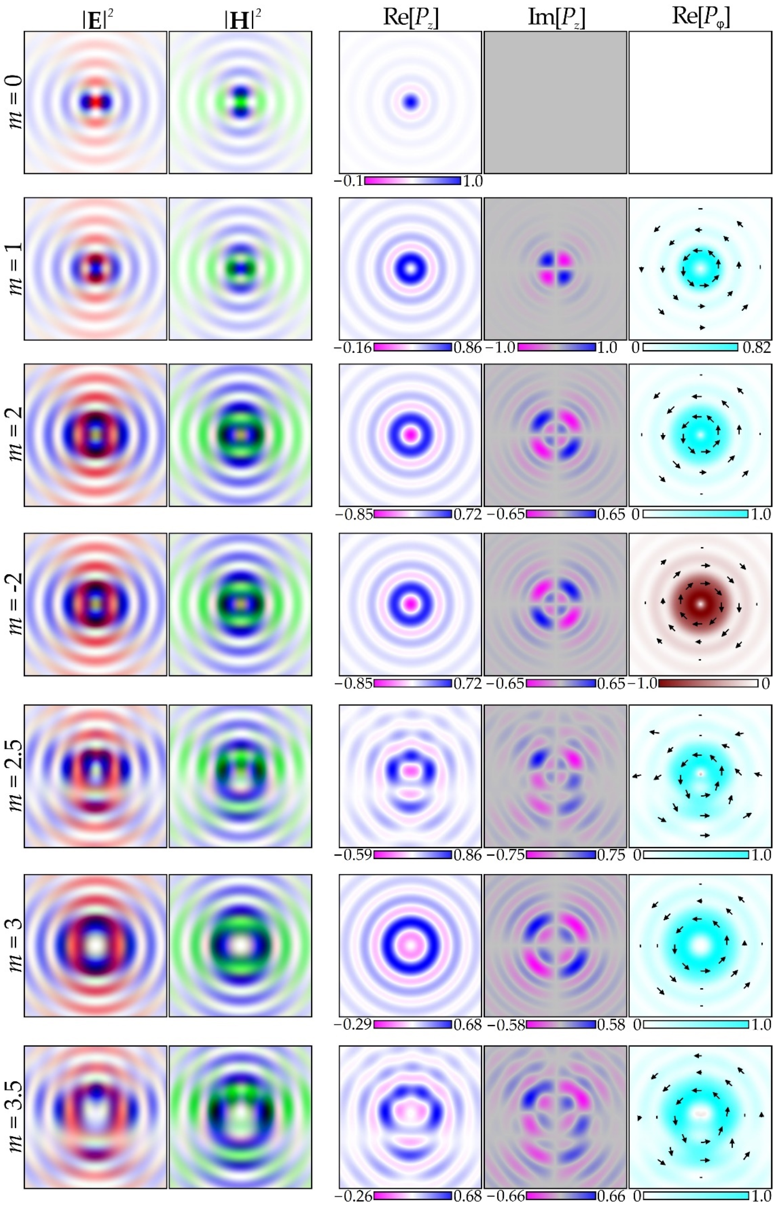
3.2. Determination of Conditions for Inverse Energy Flow on the Optical Axis

If the goal is to obtain inverse energy flow on the optical axis, then the conditions for this are different. In this case, Equation (20) takes the simple form g′(φ) = 0. Thus, the g(φ) function is decisive. Figure 1 shows an example of a graph of a function with two extrema (two stationary points).
For definiteness, assume that p 1 < 0 (the first stationary point is the maximum) and p 2 > 0 (the second is the minimum). Moreover, to simplify calculations, assume that | p 1 | = | p 2 | = p . Then, from Equation (19), we obtain the following:
Re [ P z ] 2 π p [ 2 cos θ 0 + [ 2 cos θ 0 + ( 1 cos θ 0 ) 2 sin 2 ( φ 1 φ 2 ) ] sin ( p 1 p 2 ) ] .
Equation (21) shows that the inequality sin(p1p2) < 0 must be satisfied to obtain negative values. If so, then sin21 − φ2) should be increasing. For fixed p , the minimum value of Pz is found if we have the following:
[ sin ( p 1 p 2 ) = 1 ] & [ sin ( φ 1 φ 2 ) = ± 1 ] .
In this case, it follows from Equation (21) that we get the following:
P z , min = 2 π p ( 1 cos θ 0 ) 2 .
This value is negative for any θ0, even in the paraxial case.
Thus, Equation (22) is the main result of this section and defines the condition for the inverse energy flow on the optical axis for a purely phase input field defined by Equation (10).
The conditions defined by Equation (22) mean that the difference between the values of function g(φ) at the maximum and minimum must equal 3π/2 + 2πN, and the distance between the positions of the extrema must equal π/2 or 3π/2. Considering that we need to make p smaller, it is better to choose a difference of 3π/2 (n = 0) and a distance of 3π/2.
The above reasoning shows a certain inconsistency between the desire to enhance the inverse energy flow by decreasing the value of p′′ (see Equation (23)) inaccuracy increasing of the stationary phase method in this case in this case. Thus, we have no guarantee that the phase satisfying condition defined by Equation (22) will be optimal. Therefore, the final conclusion will be made on the basis of numerical modeling by using exact Equation (9).

3.3. Determination of Conditions for Off-Axis Inverse Energy Flow

The general reasoning given in Section 3.1, as well as previous studies [17,18], shows that off-axis inverse energy flow can be greater than on the axis. This can be theoretically justified by using Equation (20) for the full phase p(φ):
p ( φ ) = g ( φ ) + k r sin θ 0 cos ( φ γ ) = g ( φ ) + μ cos ( φ γ ) , p ( φ ) = g ( φ ) μ sin ( φ γ ) , p ( φ ) = g ( φ ) μ cos ( φ γ ) .
As follows from Equation (24), for μ ≠ 0 (i.e., outside the optical axis), at least at one stationary point, p , becomes less than for μ = 0. In general, it is impossible to obtain specific results, so we consider some examples below.

3.4. Analysis of Special Cases and Simulation Results

This section discusses various specific examples and special cases of GSPP. In special cases, it is much easier to carry out theoretical analysis, so in this section, we consider not only the longitudinal but also the transverse components of the Poynting vector, as well as account for not only the real but also the imaginary part of the Poynting vector, which contributes to the transverse force acting on optically trapped Mie particles [29,30]. In the simulation, the following calculation parameters were used: the annular aperture had a central radius θ0 = 80° and width Δ = 20°.

3.4.1. Example 1: Classic SPP

First, consider the case of a standard SPP with a phase:
g ( φ ) = m φ ,
where m is an arbitrary real number.
For integer m, the calculations in Equations (11) and (12) are performed analytically and give the following result:
P z = Re [ P z ] + i Im [ P z ] = = [ π 2 ( 1 + cos θ 0 ) 2 J m 2 ( ρ ) ( π 2 / 2 ) ( 1 cos θ 0 ) 2 ( J m + 2 2 ( ρ ) + J m 2 2 ( ρ ) ) ] i [ π 2 sin 2 θ 0 sin 2 γ J m ( ρ ) ( J m + 2 ( ρ ) J m 2 ( ρ ) ) ] ,
P r = i Im [ P r ] = i π 2 sin θ 0 cos 2 γ [ ( 1 + cos θ 0 ) J m ( ρ ) ( J m 1 ( ρ ) J m + 1 ( ρ ) ) + + 0.5 ( 1 cos θ 0 ) ( J m 1 ( ρ ) J m + 2 ( ρ ) J m + 1 ( ρ ) J m 2 ( ρ ) ) ] ,
P γ = Re [ P γ ] + i Im [ P γ ] = π 2 sin θ 0 { ( 1 + cos θ 0 ) J m ( ρ ) [ J m 1 ( ρ ) + J m + 1 ( ρ ) ] + + ( 1 cos θ 0 ) [ J m 2 ( ρ ) J m 1 ( ρ ) + J m + 1 ( ρ ) J m + 2 ( ρ ) ] } + + i π 2 sin θ 0 sin 2 γ { ( 1 cos θ 0 ) [ J m 1 ( ρ ) J m + 2 ( ρ ) J m + 1 ( ρ ) J m 2 ( ρ ) ] ( 1 + cos θ 0 ) J m ( ρ ) [ J m 1 ( ρ ) J m + 1 ( ρ ) ] } ,
where ρ = krsinθ0.
As seen from Equation (26), the real part of the longitudinal component of the Poynting vector Re[Pz] has radial symmetry and does not change when m changes sign. When the sign of m changes, the imaginary part Im[Pz] changes its sign to the opposite and, for any m, has rotational symmetry of the second order due to the presence of an angular dependence sin(2γ). A negative value for Re[Pz] at the origin occurs only at m = ± 2. For m = 0 and m = ± 1, the results have a simpler form. In particular, for m = 0 Re [ P z ] = π 2 ( 1 + cos θ 0 ) 2 J 0 2 ( ρ ) π 2 ( 1 cos θ 0 ) 2 J 2 2 ( ρ ) , Im[Pz] = 0, and for m = ±1 Re [ P z ] = π 2 ( 1 + cos θ 0 ) 2 J 1 2 ( ρ ) ( π 2 / 2 ) ( 1 cos θ 0 ) 2 [ J 1 2 ( ρ ) + J 3 2 ( ρ ) ] , Im [ P z ] = π 2 sin 2 θ 0 sin 2 γ J 1 ( ρ ) [ J 1 ( ρ ) + J 3 ( ρ ) ] .
The radial component, as follows from Equation (27), is purely imaginary. Equation (28) shows that the real part of the azimuthal component Re[Pγ] is radially symmetric and equal to zero at m = 0.
It is more difficult to obtain analytical expressions for fractional values of m (as a rule, the representation through the sum for integer m is used), and they will be less descriptive. Therefore, we consider only the simulation results for these fractional values. Figure 2 shows the simulation results for standard integer and fractional SPPs with a transmission function of exp(imφ).
The distributions of the intensity of the electric |E|2 and magnetic |H|2 components of the field in the focal plane (z = 0), the distributions of individual components of the Poynting vector, the real and imaginary parts of the longitudinal component, and the real part of the angular component are shown. The longitudinal component is the main focus of this study, so we consider it comprehensively. The angular component of the Poynting vector is closely related to the angular momentum of the field, which is often formed by using SPP.
The simulation results for integer m fully correspond to analytical Equations (26) and (28). In particular, the real part of Pz has radial symmetry, and the imaginary part Pz has a structure corresponding to sin(2γ). Fractional orders of m lead to distortion of the mentioned symmetries. However, for Im[Pz], there is complete symmetry of negative and positive values for any m, which leads to a zero mean value of the imaginary part. Nevertheless, locally, it can affect optically trapped Mie particles [29,30] and for m = ± 1, the local maxima have the greatest value.
The maximum relative negative value for Re[Pz] is observed when m = 2 and it is located at the origin. Note that, for integer m, the distribution of the real part Pz is structurally similar to that for radial polarization of the mth order [17]. In both cases, the generated distributions are radially symmetric and there is a negative value on the axis only for m = 2. However, there are some differences: for radial polarization, the distribution changes slightly when the sign of m changes; when m = 1, there are no negative values. For the imaginary part, the difference is fundamental: for radial polarization, Im[Pz] = 0, and for linear polarization for classic SPPs, Im[Pz] ≠ 0 for any m ≠ 0 (see Figure 2). Obviously, for negative values of m, the results are similar; however, Im[Pz] and Re[Pγ] change signs (compare the lines in Figure 2 corresponding to m = 2 and m = −2).
In Reference [18], superposition 0.5[exp(imφ) + exp(–imφ)] = cos(mφ) was investigated. The case m = ± 2 was also noted as special in terms of maximum negative values Re[Pz] on the optical axis. However, References [17,18] also pointed out the meaning of using an illuminating beam cos(mφ) at |m| > 2, since this allows us to increase the total area and energy of negative regions. The use of fractional values of m allows for continuous changes in the properties of these areas, including changing their shape. Below, Example 2 shows that, for sin(mφ), there is a similar result up to rotation.

3.4.2. Example 2: Amplitude Spiral Plate with a Phase Shift

Consider a spiral plate defined as follows:
F 0 ( φ ) = sin ( m φ + φ 0 ) .
Add to it a phase corresponding to the compensation of the kernel phase defined by Equation (1):
g ( φ ) = α cos ( φ ) ,
where α is an arbitrary real number.
Then, p(φ) = –αcos(φ) + μcos(φ − γ) equals zero (for γ = 0) on a ring with a radius of r0 = α/(ksinθ0). It is similar to phase compensation in the focal plane of the lens. In this case, (γ = 0, α = μ) and F 0 ( φ ) = 1, and all quantities included in Equation (12) are calculated exactly:
E x * 0 2 π A ( θ 0 , φ ) d φ = π ( 1 + cos θ 0 ) , E y * 0 2 π C ( θ 0 , φ ) d φ = 0 , H y 0 2 π B ( θ 0 , φ ) d φ = π ( 1 + cos θ 0 ) , P z E x * H y | E y | 2 = π 2 ( 1 + cos θ 0 ) 2 > 0 .
Thus, in the considered region, the energy flux is positive.
However, the situation can be changed by using a non-unit amplitude, as was used in Reference [18]. Consider an amplitude that co-phases to C0,φ), that is, equals sin(φ)cos(φ) = 0.5 sin(2φ). This is the light field defined from Equation (29), when m = 2 and φ0 = 0. In this case we have the following:
E x * 0 2 π sin φ cos φ A ( θ 0 , φ ) d φ = 0 , E y * 0 2 π sin φ cos φ C ( θ 0 , φ ) d φ = π 4 ( 1 cos θ 0 ) , H y 0 2 π sin φ cos φ B ( θ 0 , φ ) d φ = 0 , P z E x * H y | E y | 2 = π 2 16 ( 1 cos θ 0 ) 2 < 0 .
Thus, in this case, the energy flow is inverse. Consider the amplitude defined by Equation (29) and the phase defined by Equation (30) together:
F 0 ( φ ) = sin ( 2 φ ) exp [ i α cos ( φ ) ] .
For a field defined by Equation (33), using the tabular formulas Section 2.5.27 in Reference [43]) gives the following in the explicit form:
E x * = 0 , H y = 0 , E y * = 2 π ( 1 cos θ 0 ) [ J 0 ( α μ ) J 4 ( α μ ) ] .
Equation (34) shows that, for γ = 0, the energy flux is negative and equal:
P z a π 2 ( 1 cos θ 0 ) 2 [ J 0 ( α k r sin θ 0 ) J 4 ( α k r sin θ 0 ) ] 2 .
Note that the imaginary part Im[Pz] in this case is equal to zero. Substituting α = 0 (there is no phase) gives an expression that coincides with the solution obtained in Reference [18] for the amplitude cos(2φ). Then an inverse flux was observed on rays corresponding to γ = ±π/4. At α ≠ 0, the phase g(φ) = –αcos(φ) plays a role similar to the linear phase with a spatial carrier (analogue of a prism): it shifts the center of the distribution from the radius r = 0 to the radius r0 = α/(ksinθ0). Figure 3 shows the corresponding simulation results. An analytical calculation for integer m shows that Pz is real, but Pγ is purely imaginary.
The results for integer m are similar to those obtained in Reference [18] for the amplitude cos(mφ) up to rotation. However, the introduction of an additional phase was not considered in Reference [18]. Such a phase does not change the main characteristics of the Poynting vector, but allows the center of the distribution to be shifted from the optical axis in accordance with Equation (35). This is important because the maximum negative value has so far been observed only at the origin of coordinates [17,18,19].
It can be seen that Im[Pz] and Re[Pγ] are nonzero only for fractional values of m in the amplitude; however, the average value also remains zero. Note also that, in examples with a half-integer frequency, the distribution Re[Pz] has two axes of symmetry and two positive maxima. Perhaps this is because half-integer frequencies retain some properties of integers, in particular, equality sin(m2π) = 0. Therefore, some features may appear, as was observed in parabolic beams [44].

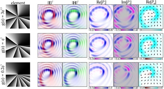
3.4.3. Example 3: Power-Exponent Phase Plate

A PEPP [40,41] has the following phase profile:
g ( φ ) = m φ s ,
where m is an arbitrary real number and s is a positive real number.
The light field formed by the plate with phase defined by Equation (36) can be represented by an infinite sum of fields formed by classic integer-order SPPs. Therefore, analytical formulas do not give a visual representation of the properties of the generated field, but References [9,10] showed that the line of maximum intensity has the shape of a spiral. In the paraxial mode, Re[Pz] is proportional to the field intensity.
Figure 4 shows the modeling results for PEPP defined by Equation (36).
Our analysis of the results shown in Figure 4 reveals that, as in Example 1 (classic SPP), the lines of the level of the real parts of Pz and Pγ are approximately parallel to the mentioned spiral: for the imaginary part of Pz, this is expressed less clearly, since sector dependence is imposed, although not as explicitly as in Example 1. Moreover, Im[Pz] no longer has symmetry of negative and positive values; however, the zero mean value of the imaginary part may remain.

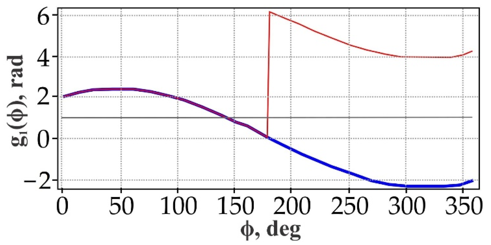
3.4.4. Example 4: Light Fields Resulting from the Stationary Phase Method

In Section 3.1, we considered the problem of the formation of an inverse flow on the optical axis within the framework of the stationary phase method. The conditions for maximizing the negative value of Re[Pz] on the optical axis, imposed on the phase function, were formulated at the end of Section 3.2. These conditions, for example, are satisfied by a function of the following form (see Figure 1):
g 1 ( φ ) = 3 π 4 sin [ 2 3 ( φ + π 2 ) ] .
Figure 5 shows the simulation results for the input field, which is a narrow ring with a phase function g1(φ) from Equation (37).
The two functions defined by the following polynomials have similar properties:
g 2 ( φ ) = 2 27 ( φ π ) 3 π 2 8 ( φ π ) .
g 3 ( φ ) = 8 9 π 2 ( φ π ) 3 3 2 ( φ π ) .
All three functions have a maximum value at a point φ1 = π/4 and a minimum value at a point φ2 = 7π/4. The first and second functions have the same values of the second derivatives at these points, but the difference, gmaxgmin = π3/8, is less than the value of 3π/2 mentioned in Section 3.2, which is in the first function. The third function has a difference of 3π/2, but the second derivatives at the extrema are slightly larger in absolute value than those of the first and second functions. Figure 6 shows graphs of all three functions. The figured shows they are very close and, therefore, will give similar results.
As follows from the calculation results shown in Figure 5, predictions based on the stationary phase method did not give the expected effect: negative values of the energy flux are small and, moreover, are mainly observed off-axis. Obviously, this is due to the approximation of the stationary phase method and, possibly, not the full legitimacy of its use.
Significant changes can be expected if the amplitude is made to equal zero outside the vicinity of the extremum points, but this entails a loss of the incident beam energy. Therefore, it is more efficient to make the second derivative equal zero (although the stationary phase method is no longer directly applicable here), i.e., to use the binary version of the considered phase functions, as shown in the following example.

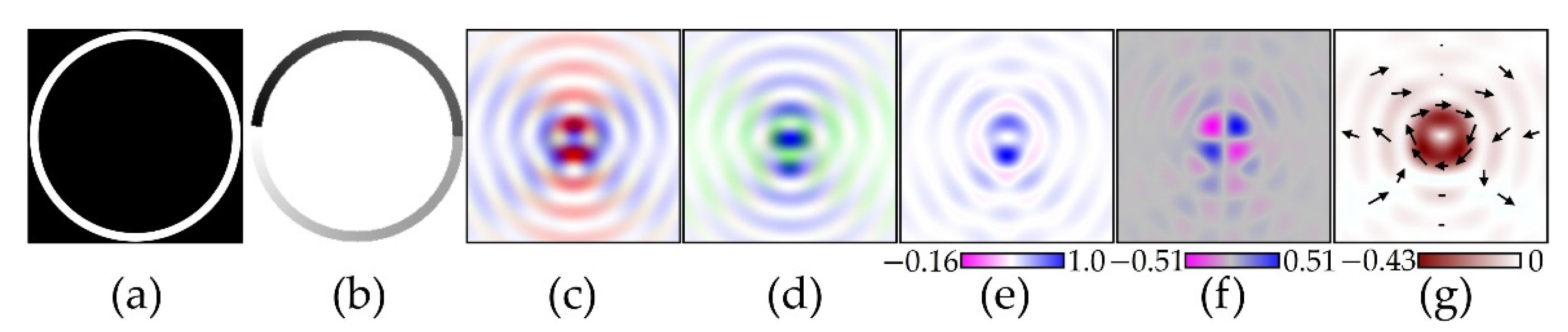
3.4.5. Example 5: Binary Phase

Reference [18] showed that the distribution of the Poynting vector changes little if the incident beam with amplitude cos(mφ) is replaced by a beam with unit amplitude and binary phase.
Therefore, consider a phase function of the following form:
g b ( φ ) = π sgn [ sin ( m φ + φ 0 ) ] / 2 + h .
where sgn ( ) is the sign function and h is a real constant. In contrast to Reference [18], m can be a non-integer. Obviously, parameters φ0 and h do not qualitatively affect the distribution pattern: φ0 determines its rotation, and h should not change it at all, but h ≠ 0 may be more convenient when carrying out an experiment. The simulation results for binary phase functions defined by Equation (40) for various values of m are shown in Figure 7.
Comparing Figure 3 and Figure 7 reveals that the distributions in the focal plane for the binary phases strongly correlate with distributions for the amplitude in the form of a sine, as it is actually supposed to be. There are two main differences: the spots have slightly changed their shape and the energy efficiency is increased.

4. Discussion

The obtained analytical and numerical results allow us to draw some conclusions about the preferred variants of the input field for amplifying the reverse energy flow in different areas of the focal plane.
Obviously, to ensure the reverse energy flow, Equation (5) must take negative values in a certain area. However, if the specific form of the fields participating in Equation (5) is unknown, it is impossible to make any assumptions. Note that Equation (5) includes the field distributions in the focal region; therefore, it is difficult to guess what the initial field (in the input plane) should be to achieve this goal. To do this, it would be necessary to solve the inverse problem for vector fields taking into account Maxwell’s equations, which is difficult in general form. Therefore, we have limited the consideration to a certain class of input fields. In particular, the field was assumed to be linearly polarized. This made it possible to reduce the general Equation (5) to a particular Equation (12), which is more illustrative for the search for possible solutions. Moreover, to perform analytical calculations, we considered the input field in the form defined by Equation (7), imposing a narrow annular aperture, and thus obtained a dependence on only one variable.
The imposition of such restrictions allowed us to apply the stationary phase method to calculate the integrals and obtain condition defined by Equation (22) for inverse energy flow on the optical axis for a purely phase input field (the amplitude is constant). However, due to the approximation of the stationary phase method, which is especially manifested on the optical axis, the obtained analytical functions for the input field did not give a large value of the inverse energy flow. However, the analysis based on the stationary phase method suggested that the inverse energy flow out of the optical axis may be greater than at the axis.
Due to the limitations of the stationary phase method, we proceeded to the analysis of exact expressions for several types of the input field. Among the considered fields, two types are special: (1) the classical spiral phase plate of the second order g(φ) = 2φ, which provides the maximum inverse energy flow on the optical axis; and (2) a generalized spiral phase plate g(φ) = −αcos(φ + φ1) with the amplitude sin[2(φ + φ2)], which forms regions of the inverse energy flow with a larger size and allows this region to be displaced.

5. Conclusions

Structured laser beams with the predetermined amplitude, phase, and polarization distributions play an important role in the field of laser manipulation. The possibility to form light fields with the desired distribution of the Poynting vector representing the directional energy flux of an electromagnetic field allows one to affect optically trapped particles in a controlled manner. In this paper, we demonstrated the possibility to form light fields with an inverse energy flux and control the distributions of the real and imaginary parts of the Poynting vector, using conventional and GSPPs illuminated with linearly polarized laser radiation. Our theoretical analysis based on the stationary phase method provides the conditions for generating inverse energy flux on the optical axis in the case of conventional and generalized SPPs. We also obtained the conditions for maximizing the negative value of the real part of the longitudinal component of the Poynting vector.
We showed that, for a classic SPP exp(imφ), the maximum relative negative value for the real part of the longitudinal component of the Poynting vector is observed when m = 2 and it is located at the origin. In addition, for integer m, the real part of the longitudinal component has radial symmetry, and the imaginary part of the longitudinal component has a structure corresponding to sin(2φ). The use of a special phase allows us to shift the center of the Poynting vector distribution from the optical axis, so the maximum negative value of the inverse energy flux will be out of the origin of coordinates. The use of PEPPs allows us to break the symmetry of negative and positive values of the imaginary part of the longitudinal component of the Poynting vector; however, the zero mean value of the imaginary part may remain. Currently, laser sources with a linearly polarized output radiation are the most readily available, which makes the results obtained in this work attractive for use in the field of laser manipulation.

Author Contributions

Conceptualization, S.N.K.; methodology, S.N.K. and A.V.U.; software, S.N.K.; validation, S.N.K. and A.P.P.; formal analysis, S.N.K. and A.V.U.; investigation, S.N.K. and A.P.P.; writing—original draft preparation, S.N.K. and A.P.P.; writing—review and editing, S.N.K. and A.P.P.; supervision, S.N.K.; funding acquisition, A.P.P. All authors have read and agreed to the published version of the manuscript.

Funding

This research was funded by the Russian Foundation for Basic Research (grant number 20-37-70025) and Russian Federation Ministry of Science and Higher Education (007-GZ/Ch3363/26).

Institutional Review Board Statement

Not applicable.

Informed Consent Statement

Not applicable.

Data Availability Statement

Not applicable.

Conflicts of Interest

The authors declare that there are no conflict of interest related to this article.

References

  1. Higgins, T.V. Spiral waveplate design produces radially polarized laser light. Laser Focus World 1992, 28, 18–20. [Google Scholar]
  2. Beijersbergen, M.W.; Coerwinkel, R.C.; Kristensen, M.; Woerdman, J.P. Helical-wavefront laser beams produced with a spiral phase plate. Opt. Commun. 1994, 112, 321–327. [Google Scholar] [CrossRef]
  3. Moh, K.J.; Yuan, X.-C.; Tang, D.Y.; Cheong, W.C.; Zhang, L.S.; Low, D.K.Y.; Peng, X.; Niu, H.B.; Lin, Z.Y. Generation of femtosecond optical vortices using a single refractive optical element. Appl. Phys. Lett. 2006, 88, 091103. [Google Scholar] [CrossRef]
  4. Berry, M.V. Optical vortices evolving from helicoidal integer and fractional phase steps. J. Opt. A Pure Appl. Opt. 2004, 6, 259–268. [Google Scholar] [CrossRef]
  5. Luo, M.; Wang, Z. Fractional vortex ultrashort pulsed beams with modulating vortex strength. Opt. Express 2019, 27, 36259–36268. [Google Scholar] [CrossRef]
  6. Khonina, S.; Karpeev, S.; Butt, M. Spatial-Light-Modulator-Based Multichannel Data Transmission by Vortex Beams of Various Orders. Sensors 2021, 21, 2988. [Google Scholar] [CrossRef] [PubMed]
  7. Li, P.; Liu, S.; Peng, T.; Xie, G.; Gan, X.; Zhao, J. Spiral autofocusing Airy beams carrying power-exponent-phase vortices. Opt. Express 2014, 22, 7598–7606. [Google Scholar] [CrossRef]
  8. Lao, G.; Zhang, Z.; Zhao, D. Propagation of the power-exponent-phase vortex beam in paraxial ABCD system. Opt. Express 2016, 24, 18082–18094. [Google Scholar] [CrossRef]
  9. Khonina, S.N.; Ustinov, A.V.; Logachev, V.I.; Porfirev, A.P. Properties of vortex light fields generated by generalized spiral phase plates. Phys. Rev. A 2020, 101, 043829. [Google Scholar] [CrossRef]
  10. Ustinov, A.V.; Khonina, S.N.; Khorin, P.A.; Porifrev, A.P. Control of the intensity distribution along the light spiral generated by a generalized spiral phase plate. J. Opt. Soc. Am. B 2021, 38, 420. [Google Scholar] [CrossRef]
  11. Shanblatt, E.R.; Grier, D.G. Extended and knotted optical traps in three dimensions. Opt. Express 2011, 19, 5833–5838. [Google Scholar] [CrossRef]
  12. Rodrigo, J.A.; Alieva, T.; Abramochkin, E.; Castro, I. Shaping of light beams along curves in three dimensions. Opt. Express 2013, 21, 20544–20555. [Google Scholar] [CrossRef] [Green Version]
  13. Woerdemann, M.; Alpmann, C.; Esseling, M.; Denz, C. Advanced optical trapping by complex beam shaping. Laser Photon- Rev. 2013, 7, 839–854. [Google Scholar] [CrossRef]
  14. Bekshaev, A.; Soskin, M. Transverse energy flows in vectorial fields of paraxial beams with singularities. Opt. Commun. 2007, 271, 332–348. [Google Scholar] [CrossRef]
  15. Bekshaev, A.Y. Internal energy flows and instantaneous field of a monochromatic paraxial light beam. Appl. Opt. 2012, 51, C13–C16. [Google Scholar] [CrossRef] [PubMed]
  16. Novitsky, A.; Novitsky, D. Negative propagation of vector Bessel beams. J. Opt. Soc. Am. A 2007, 24, 2844–2849. [Google Scholar] [CrossRef]
  17. Khonina, S.N.; Ustinov, A.V.; Degtyarev, S. Inverse energy flux of focused radially polarized optical beams. Phys. Rev. A 2018, 98, 043823. [Google Scholar] [CrossRef]
  18. Khonina, S.N.; Ustinov, A.V. Increased reverse energy flux area when focusing a linearly polarized annular beam with binary plates. Opt. Lett. 2019, 44, 2008–2011. [Google Scholar] [CrossRef]
  19. Kotlyar, V.V.; Stafeev, S.S.; Nalimov, A.G.; Kovalev, A.A.; Porfirev, A.P. Mechanism of formation of an inverse energy flow in a sharp focus. Phys. Rev. A 2020, 101, 033811. [Google Scholar] [CrossRef]
  20. Zemánek, P.; Volpe, G.; Jonáš, A.; Brzobohatý, O. Perspective on light-induced transport of particles: From optical forces to phoretic motion. Adv. Opt. Photon. 2019, 11, 577–678. [Google Scholar] [CrossRef]
  21. Saenz, J.J. Laser tractor beams. Nat. Photon. 2011, 5, 514–515. [Google Scholar] [CrossRef]
  22. Sukhov, S.; Dogariu, A. On the concept of ‘tractor beams’. Opt. Lett. 2010, 35, 3847–3849. [Google Scholar] [CrossRef]
  23. Novitsky, A.; Ding, W.; Wang, M.; Gao, D.; Lavrinenko, A.; Qiu, C.-W. Pulling cylindrical particles using a soft-nonparaxial tractor beam. Sci. Rep. 2017, 7, 1–10. [Google Scholar] [CrossRef] [Green Version]
  24. Lan, C.; Yang, Y.; Geng, Z.; Li, B.; Zhou, J. Electrostatic Field Invisibility Cloak. Sci. Rep. 2015, 5, 16416. [Google Scholar] [CrossRef] [Green Version]
  25. Novitsky, A.; Qiu, C.-W.; Wang, H. Single Gradientless Light Beam Drags Particles as Tractor Beams. Phys. Rev. Lett. 2011, 107, 203601. [Google Scholar] [CrossRef] [Green Version]
  26. Qiu, C.-W.; Palima, D.; Novitsky, A.; Gao, D.; Ding, W.; Zhukovsky, S.; Gluckstad, J. Engineering light-matter interaction for emerging optical manipulation applications. Nanophotonics 2014, 3, 181–201. [Google Scholar] [CrossRef]
  27. Wong, V.; Ratner, M.A. Explicit computation of gradient and nongradient contributions to optical forces in the discrete-dipole approximation. J. Opt. Soc. Am. B 2006, 23, 1801–1814. [Google Scholar] [CrossRef]
  28. Novitsky, A.; Qiu, C.-W. Pulling extremely anisotropic lossy particles using light without intensity gradient. Phys. Rev. A 2014, 90, 053815. [Google Scholar] [CrossRef] [Green Version]
  29. Bliokh, K.; Bekshaev, A.Y.; Nori, F. Extraordinary momentum and spin in evanescent waves. Nat. Commun. 2014, 5, 3300. [Google Scholar] [CrossRef]
  30. Bekshaev, A.Y.; Bliokh, K.; Nori, F. Transverse Spin and Momentum in Two-Wave Interference. Phys. Rev. X 2015, 5, 011039. [Google Scholar] [CrossRef]
  31. Xu, X.; Nieto-Vesperinas, M. Azimuthal Imaginary Poynting Momentum Density. Phys. Rev. Lett. 2019, 123, 233902. [Google Scholar] [CrossRef]
  32. Khonina, S.N.; Degtyarev, S.A.; Ustinov, A.V.; Porfirev, A.P. Metalenses for the generation of vector Lissajous beams with a complex Poynting vector density. Opt. Express 2021, 29, 18634–18645. [Google Scholar] [CrossRef]
  33. Richards, B.; Wolf, E. Electromagnetic diffraction in optical systems, II. Structure of the image field in an aplanatic system. Proc. R. Soc. London. Ser. A Math. Phys. Sci. 1959, 253, 358–379. [Google Scholar] [CrossRef]
  34. Pereira, S.; van de Nes, A. Superresolution by means of polarisation, phase and amplitude pupil masks. Opt. Commun. 2004, 234, 119–124. [Google Scholar] [CrossRef]
  35. Khonina, S.; Ustinov, A.V.; Volotovsky, S.G. Shaping of spherical light intensity based on the interference of tightly focused beams with different polarizations. Opt. Laser Technol. 2014, 60, 99–106. [Google Scholar] [CrossRef]
  36. Jackson, J.D.; Levitt, L.C. Classical Electrodynamics. Phys. Today 1962, 15, 62. [Google Scholar] [CrossRef] [Green Version]
  37. Cameron, R.P.; Speirits, F.C.; Gilson, C.R.; Allen, L.; Barnett, S.M. The azimuthal component of Poynting’s vector and the angular momentum of light. J. Opt. 2015, 17, 125610. [Google Scholar] [CrossRef] [Green Version]
  38. Ustinov, A.V.; Niziev, V.G.; Khonina, S.N.; Karpeev, S.V. Local characteristics of paraxial Laguerre–Gaussian vortex beams with a zero total angular momentum. J. Mod. Opt. 2019, 66, 1961–1972. [Google Scholar] [CrossRef]
  39. Sheppard, C.J.R.; Choudhury, A. Annular pupils, radial polarization, and superresolution. Appl. Opt. 2004, 43, 4322–4327. [Google Scholar] [CrossRef] [PubMed]
  40. Khonina, S.N. Vortex beams with high-order cylindrical polarization: Features of focal distributions. Appl. Phys. A 2019, 125, 100. [Google Scholar] [CrossRef]
  41. Fedoruk, M.V. Asymptotics Integral and Series; Nauka: Moscow, Russia, 1987. [Google Scholar]
  42. Friberg, A.T. Stationary-phase analysis of generalized axicons. J. Opt. Soc. Am. A 1996, 13, 743–750. [Google Scholar] [CrossRef]
  43. Prudnikov, A.; Brychkov, Y.A.; Marichev, O. Integrals and Series; Informa UK Limited: London, UK, 2018; Volume 1. [Google Scholar]
  44. Khonina, S.N.; Ustinov, A.V.; Porfirev, A.P. Fractional two-parameter parabolic diffraction-free beams. Opt. Commun. 2019, 450, 103–111. [Google Scholar] [CrossRef]
Figure 1. Function g1(φ): original function (blue curve) and function reduced to positive values (red curve).
Photonics 08 00283 g001
Figure 2. Simulation results for classic SPPs exp(imφ) of various orders m (red color—for x-components, green color—for y-components, and blue color—for z-components). The distributions in the focal plane with a size of 4λ × 4λ are shown.
Photonics 08 00283 g002
Figure 3. Simulation results for amplitude spiral plates (red color—for x-components, green color—for y-components, and blue color—for z-components). The distributions in the focal plane with a size of 4λ × 4λ are shown.
Photonics 08 00283 g003
Figure 4. Simulation results for PEPPs exp(imϕs) (red color—for x-components, green color—for y-components, and blue color—for z-components). The distributions in the focal plane with a size of 6λ × 6λ are shown.
Photonics 08 00283 g004
Figure 5. Simulation results for the input field with phase g1(φ) defined from Equation (37): amplitude (a) and phase (b) distribution of the input field; |E|2 (c) and |H|2 (d) distributions in the focal plane, as well as the distributions of Re[Pz] (e), Im[Pz] (f), and Re[Pγ] (g).
Photonics 08 00283 g005
Figure 6. Phase functions: g1(φ) defined by Equation (37) (blue line), g2(φ) defined by Equation (38) (green line), and g3(φ) defined by Equation (39) (red line).
Photonics 08 00283 g006
Figure 7. Simulation results for binary phases (red color—for x-components, green color—for y-components, and blue color—for z-components). The distributions in the focal plane with a size of 4λ × 4λ are shown.
Photonics 08 00283 g007
Publisher’s Note: MDPI stays neutral with regard to jurisdictional claims in published maps and institutional affiliations.

