Single-Port Homodyne Detection in a Squeezed-State Interferometry with Optimal Data Processing

Abstract

Performing homodyne detection at a single output port of a squeezed-state light interferometer and then separating the measurement quadrature into several bins can realize superresolving and supersensitive phase measurements. However, the phase resolution and the achievable phase sensitivity depend on the bin size that is adopted in the data processing. By maximizing classical Fisher information, we analytically derive an optimal value of the bin size and the associated best sensitivity for the case of three bins, which can be regarded as a three-outcome measurement. Our results indicate that both the resolution and the achievable sensitivity are better than that of the previous binary–outcome case. Finally, we present an approximate maximum Likelihood estimator to asymptotically saturate the ultimate lower bound of the phase sensitivity.

1. Introduction

High-precision phase measurement is of importance for multiple areas of scientific research, such as gravitational wave detection [1,2], biological sensing [3,4], atomic clocks [5,6], and magnetometry [7]. For instance, the intensity measurements at the output ports of a coherent-state light interferometer show the interferometric signal $\propto {sin}^2(\theta /2)$ or ${cos}^2(\theta /2)$, where $\theta$ is a dimensionless phase shift. Obviously, the signal exhibits the full width at half maximum ($\mathrm{FWHM}$) $=\pi$, corresponding to the fringe resolution $\sim \lambda /2$, where $\lambda$ is the wavelength of the incident light. This is known as the so-called Rayleigh resolution limit [8]. On the other hand, the achievable phase sensitivity is subject to the shot-noise limit (SNL) $\delta {\theta }_{\mathrm{SNL}}=1/\sqrt{\overline{n}}$, where $\overline{n}$ is the number of particles of the input state.

As proposed originally by Caves [9], the best sensitivity of the interferometer can beat the SNL by mixing a small amount of squeezed vacuum with the coherent-state light at the input ports of the interferometer (named hereinafter, squeezed-state interferometer). Performing homodyne detections at one output port of the interferometer and following with a suitable data processing, Schäfermeier et al. [10] recently demonstrated that the two classical limits in the resolution and in the sensitivity can be surpassed simultaneously. The data processing method adopted in Ref. [10] is to divide the measurement outcomes into two discrete bins and then construct an inversion estimator associated with one discrete outcome [11]. The inversion estimator is widely used in experiments since its uncertainty simply follows the error-propagation formula [12]. However, the inversion estimator is usually sub-optimal and cannot saturate the ultimate phase estimation precision that determined by the Cramér–Rao lower bound (CRB) [13,14,15,16,17,18,19]:

$$\delta \theta \ge \delta {\theta }_{\mathrm{CRB}}\equiv \frac{1}{\sqrt{\mathcal{F}(\theta )}},$$

(1)

where $\mathcal{F}(\theta )$ is the classical Fisher information (CFI) determined by the measurement outcome probability distribution $P_k(\theta )$:

$$\mathcal{F}(\theta )=\sum _k{f}_k(\theta ),f_k(\theta )=\frac{1}{P_k(\theta )}{\left[\frac{\partial P_k(\theta )}{\partial \theta }\right]}^2.$$

(2)

Here, the subscript k and $f_k(\theta )$ represent the k-th measurement outcome and its contribution to the CFI. The data processing method adopted in Ref. [10] can be regarded as a binary–outcome measurement with $k=0$ and ∅, corresponding to the measurement quadrature $p\in [-a,a]$ and $p\notin [-a,a]$, with the bin size $2a$. As a trade-off parameter, the different choice of a is of importance to control the phase resolution and the achievable phase sensitivity [11].

In this paper, we focus on optimal value of the bin size and present the best sensitivity of the three-outcome homodyne detections. By maximizing the CFI of the three-outcome measurement, we derive analytic expressions of the bin size and the best sensitivity. Our analytic results are useful to predict the Heisenberg scaling of the sensitivity $\delta {\theta }_{\mathrm{CRB}}\sim O(1/\overline{n})$. We perform numerical simulations of the three-outcome homodyne detections, using $\mathcal{N}$ random numbers at each given phase shift. To saturate the CRB, we adopt the approximate maximum Likelihood estimator (MLE) that developed recently by Ref. [20], which holds for any kind multi-outcome detections with discrete measurement outcomes. Our results show clearly a physical meaning of the MLE and the reason why it can saturate the CRB as $\mathcal{N}\gg 1$.

2. Homodyne Detection in the Squeezed-State Interferometer with Dataprocessing

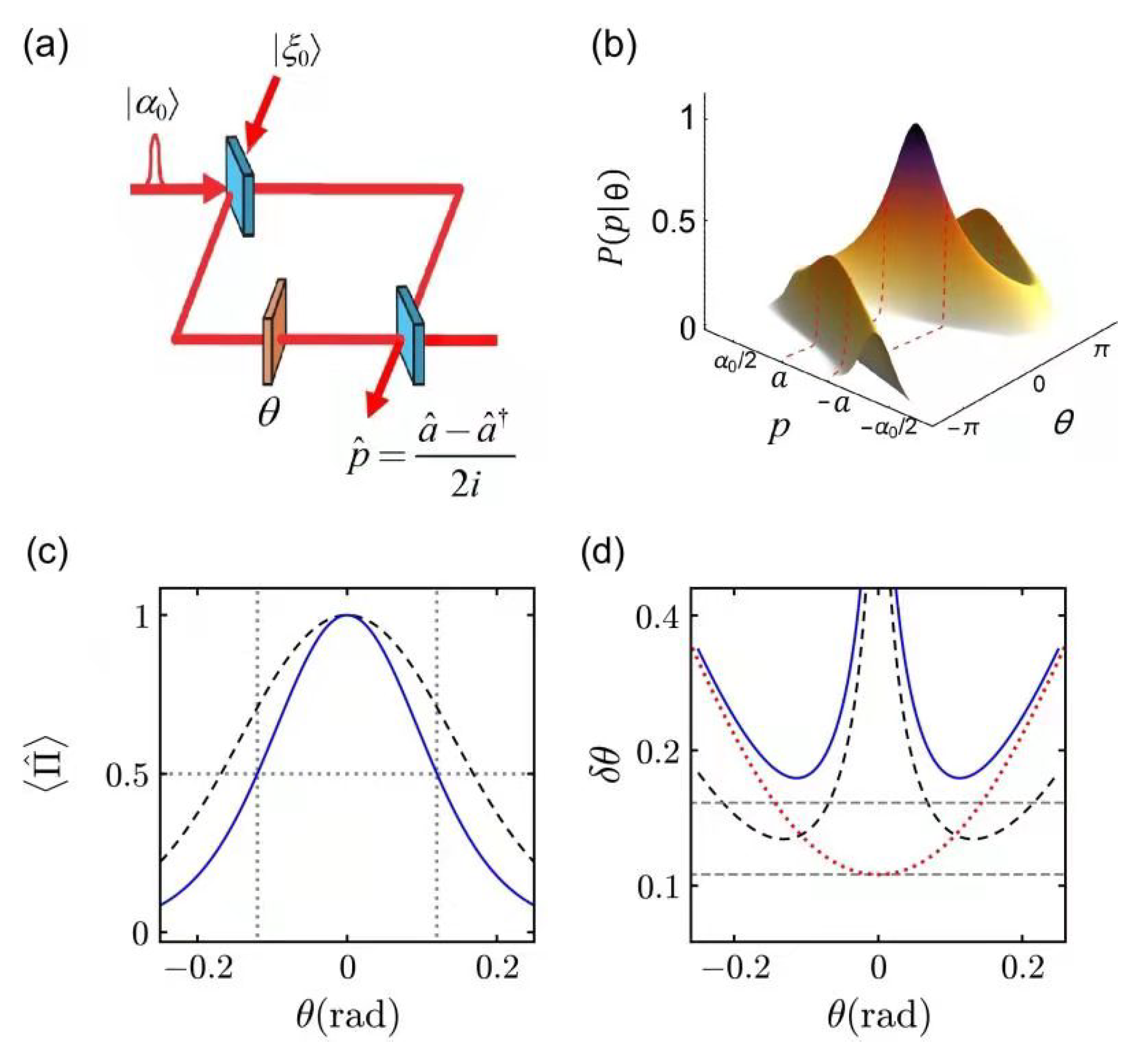
As illustrated by Figure 1a, let us consider homodyne detection at one output port of a squeezed-state light interferometer, which is equivalent to measuring the field quadrature $\widehat{p}=(\widehat{a}-{\widehat{a}}^{†})/(2i)$, where $\widehat{p}|p\rangle =p|p\rangle$ and $p\in (-\infty ,\infty )$. To improve the phase sensitivity, we choose a coherent state and a squeezed vacuum state with real field amplitudes [9,21,22,23], corresponding to the input state $|{\psi }_{\mathrm{in}}\rangle =|{\alpha }_0\rangle \otimes |{\xi }_0\rangle$, with ${\alpha }_0=\sqrt{{\overline{n}}_a}\in \mathbb{R}$ and ${\xi }_0=-r\in \mathbb{R}$. The average number of photons of the input state is given by $\overline{n}={\overline{n}}_a+{\overline{n}}_b$, with ${\overline{n}}_a={\alpha }_0^2$ and ${\overline{n}}_b={sinh}^{2}r$. The Wigner function of the input state is given by [24,25,26,27]

$$W_{\mathrm{in}}(\alpha ,\beta )=\frac{2}{\pi }{e}^{-2\left[{\left(x_a-{\alpha }_0\right)}^2+p_a^2\right]}\frac{2}{\pi }\sqrt{\tilde{\mu }\tilde{\nu }}{e}^{-2\left(\tilde{\mu }{x}_b^2+\tilde{\nu }{p}_b^2\right)},$$

(3)

with the parameters $\tilde{\mu }$ and $\tilde{\nu }$ dependent on the input state, and the variables $\alpha =x_a+i{p}_a$ and $\beta =x_b+i{p}_b$. Here, the subscripts “a” and “b” denote two different paths (or the field modes). Following Schäfermeier et al. [10], we consider the squeezed vacuum with the purity $\varrho <1$ and take $\tilde{\mu }=\varrho e^{-2r}$ and $\tilde{\nu }=\varrho e^{2r}$, where $e^{-r}$ describes the squeeze factor of $|{\xi }_0\rangle$. If other Gaussian state $|g\rangle$ is injected from the port b, then $\tilde{\mu }$ and $\tilde{\nu }$ can take different expressions (e.g., $\tilde{\mu }=\tilde{\nu }=1$ for the vacuum $|0\rangle$). Next, we consider the interferometer that is described by the unitary operator:

$$\widehat{U}(\theta )=e^{-i\pi {\widehat{J}}_y/2}{e}^{-i\theta {\widehat{a}}^{†}\widehat{a}}{e}^{-i\pi {\widehat{J}}_y/2},$$

(4)

where $exp(-i\pi {\widehat{J}}_y/2)$ and $exp(-i\theta {\widehat{a}}^{†}\widehat{a})$ represent the actions of the 50:50 beam splitter and that of the phase accumulation in the path, with ${\widehat{J}}_y=({\widehat{a}}^{†}\widehat{b}-{\widehat{b}}^{†}\widehat{a})/2i$ and $\widehat{a}$, $\widehat{b}$ being bosonic annihilation operators. According to Refs. [24,25,26,27], the Wigner function of the output state $|{\psi }_{\mathrm{out}}\rangle =\widehat{U}(\theta )|{\psi }_{\mathrm{in}}\rangle$ takes the same form with that of the input state, i.e., $W_{\mathrm{out}}(\alpha ,\beta )=W_{\mathrm{in}}({\tilde{\alpha }}_{\theta },{\tilde{\beta }}_{\theta })$, with

$$\left\{\begin{array}{c}{\tilde{\alpha }}_{\theta }=\alpha \frac{e^{i\theta }-1}{2}+\beta \frac{e^{i\theta }+1}{2},\hfill \\ {\tilde{\beta }}_{\theta }=-\alpha \frac{e^{i\theta }+1}{2}-\beta \frac{e^{i\theta }-1}{2}.\hfill \end{array}\right.$$

(5)

Integrating $W_{\mathrm{out}}(\alpha ,\beta )$ over $\{x_a$, $x_b$, $p_b\}$, one can obtain the conditional probability for detecting a measurement outcome [28]:

$$P(p|\theta )=\sqrt{\frac{2}{\pi {\eta }_{\theta }}}exp\left[-\frac{2}{{\eta }_{\theta }}{\left(p+\frac{{\alpha }_0}{2}sin\theta \right)}^2\right],$$

(6)

where the subscript of $p_a$ has been neglected, and we introduce

$${\eta }_{\theta }=\frac{1}{4\tilde{\mu }\tilde{\nu }}\left[\tilde{\mu }+\tilde{\nu }+2\tilde{\mu }\tilde{\nu }-2\tilde{\mu }(\tilde{\nu }-1)cos\theta +(\tilde{\mu }-\tilde{\nu }){cos}^2\theta \right].$$

(7)

Note that Equations (3)–(7) hold for the output state $\widehat{U}(\theta )|{\alpha }_0\rangle \otimes |g\rangle$, where $|{\alpha }_0\rangle$ denotes a coherent state and $|g\rangle$ is an arbitrary Gaussian state, as mentioned above.

In Figure 1b, we show a 3D plot of $P(p|\theta )$ against the phase shift $\theta$ and the measurement quadrature p. One can find that the conditional probability is nonzero within a region $p\in (-{\alpha }_0/2,{\alpha }_0/2)$ and $P(p|\theta )=1$ at $\theta =0$. With the single-port homodyne detection, one can easily obtain the output signal

$$\langle \widehat{p}(\theta )\rangle ={\int }_{\mathbb{R}}dpP(p|\theta )p=-\frac{{\alpha }_0}{2}sin\theta ,$$

(8)

which exhibits the $\mathrm{FWHM}=2\pi /3$, and hence the Rayleigh limit in fringe resolution [10,11]. On the other hand, the achievable phase sensitivity is determined by the CFI

$$F(\theta )={\int }_{\mathbb{R}}dpP(p|\theta ){\left[\frac{\partial lnP(p|\theta )}{\partial \theta }\right]}^2={\int }_{\mathbb{R}}dp\frac{{\left[P^{\prime }(p|\theta )\right]}^2}{P(p|\theta )},$$

(9)

and hence the CRB $1/\sqrt{F(\theta )}$ (see, e.g., Ref. [28]), where $P^{\prime }\equiv \partial P/\partial \theta$. When the coherent-state component dominates over the squeezed vacuum (i.e., ${\overline{n}}_a\gg {\overline{n}}_b$), the best sensitivity occurs at the optimal working point ${\theta }_{min}=0$, with $\delta {\theta }_{min}\equiv 1/\sqrt{F({\theta }_{min})}\approx e^{-r}/\sqrt{\overline{n}}$ [28], in agreement with the light intensity-difference measurement as ${\overline{n}}_a\gg {\overline{n}}_b$ [9,21].

The phase resolution can be improved by a suitable data processing over the measurement outcomes, at the cost of reduced phase sensitivity. Recently, Distante et al. [11] have demonstrated super-resolving phase measurement in a coherent-state light interferometer with the sensitivity close to the SNL. The data-processing method they adopted is to separate the measurement quadrature $p\in (-\infty ,\infty )$ into two bins: $p\in [-a,a]$ and $p\notin [-a,a]$, where a is to be determined. With such a kind of binary–outcome measurement, Schäfermeier et al. [10] have demonstrated super-sensitive and super-resolving phase measurement in the squeezed-state interferometer. Specifically, a 22-fold improvement in the resolution and a $1.7$-fold improvement in the sensitivity can be obtained using realistic experimental parameters [10]. A better phase resolution and an enhanced sensitivity can be obtained by dividing the measurement data into several bins, with an optimal choice of the bin size a.

Using the experimental setup similar to Schäfermeier et al. [10], one can separate the measurement data into three bins: $(-\infty ,-a)$, $[-a,a]$, and $(a,\infty )$, denoted hereinafter by the outcomes “−”, “0”, and “+”, respectively. Integrating $P(p|\theta )$ in Equation (6), one can obtain the occurrence probabilities of each outcome:

$$\left\{\begin{array}{c}{P}_{-}(\theta )={\int }_{-\infty }^{-a}dpP(p|\theta )=\frac{1}{2}(1+\mathrm{erf}\left[g_{-}(\theta )\right]),\\ P_0(\theta )={\int }_{-a}^{a}dpP(p|\theta )=\frac{1}{2}\mathrm{Erf}\left[g_{-}(\theta ),g_{+}(\theta )\right],\\ P_{+}(\theta )={\int }_a^{\infty }dpP(p|\theta )=\frac{1}{2}(1-\mathrm{erf}\left[g_{+}(\theta )\right]),\end{array}\right.$$

(10)

where $\mathrm{Erf}\left[x,y\right]\equiv \mathrm{erf}\left[y\right]-\mathrm{erf}\left[x\right]$ denotes a generalized error function, and

$$g_{\pm }(\theta )=\sqrt{\frac{2}{{\eta }_{\theta }}}\left(\frac{{\alpha }_0}{2}sin\theta \pm a\right),$$

(11)

with ${\eta }_{\theta }$ being defined by Equation (7). Note that the above data-processing method is equivalent to a three-outcome measurement with the observable $\widehat{\Pi }={\sum }_k{\mu }_k{\widehat{\Pi }}_k$, where ${\mu }_k$ are the eigenvalues associated with the outcomes $k=-$, 0, and +. Furthermore, the projection operators are given by ${\widehat{\Pi }}_{-}={\int }_{-\infty }^{-a}|p\rangle \langle p|dp$, ${\widehat{\Pi }}_0={\int }_{-a}^a|p\rangle \langle p|dp$, and ${\widehat{\Pi }}_{+}={\int }_a^{\infty }|p\rangle \langle p|dp$. Using the relation $P_k(\theta )=\langle {\psi }_{\mathrm{out}}|{\widehat{\Pi }}_k|{\psi }_{\mathrm{out}}\rangle$, one can easily obtain the averaged output signal

$$\langle \widehat{\Pi }(\theta )\rangle =\sum _k{\mu }_k{P}_k(\theta )\approx \sum _k{\mu }_k{\mathcal{N}}_k/\mathcal{N},$$

(12)

where ${\mathcal{N}}_k$ denotes the occurrence number of the kth outcome for a single run $\mathcal{N}$ independent measurements. Actually, the probability of each outcome can be measured by the occurrence frequency ${\mathcal{N}}_k/\mathcal{N}$. Performing $\mathcal{N}$ repeated measurements at each given $\theta \in (-\pi ,\pi )$, one can obtain the occurrence numbers of all the outcomes $\left\{{\mathcal{N}}_k\right\}$, which can be regarded as a single run. After multiple runs, one can obtain the phase-dependent probabilities from the statistical average of ${\mathcal{N}}_k/\mathcal{N}$, and thereby the averaged signal $g(\theta )\approx \langle \widehat{\Pi }(\theta )\rangle$. This can be done by the calibration of the interferometer (see below).

To estimate an unknown phase shift, the inversion estimator is widely used in experiments due to its simplicity, i.e., ${\theta }_{\mathrm{inv}}=g^{-1}({\sum }_k{\mu }_k{\mathcal{N}}_k/\mathcal{N})$, where $g^{-1}$ denotes the inverse function of the signal. According to the central limit theorem, the phase uncertainty of ${\theta }_{\mathrm{inv}}$ follows error–propagation formula [12]:

$$\delta \theta =\frac{\Delta \widehat{\Pi }}{\left|\partial \langle \widehat{\Pi }(\theta )\rangle /\partial \theta \right|},$$

(13)

where $\Delta \widehat{\Pi }=\sqrt{\langle {\widehat{\Pi }}^2\rangle -{\langle \widehat{\Pi }\rangle }^2}$ denotes the root-mean-square fluctuation of the signal.

Usually, the signal and the phase sensitivity depend on the choice of the eigenvalues $\left\{{\mu }_k\right\}$. Similar to Schäfermeier et al. [10], one can take ${\mu }_{\pm }=0$ and ${\mu }_0=1/\mathrm{erf}(\sqrt{2\tilde{\nu }}a)$, which leads to the maximum of the signal $\langle \widehat{\Pi }(0)\rangle ={\mu }_0{P}_0(0)=1$ (see below, Figure 1(c)). Actually, the signal and the sensitivity reduce to the binary–outcome case as long as ${\mu }_{+}={\mu }_{-}={\mu }_{\varnothing }$. With arbitrary values of ${\mu }_{\varnothing }$ and ${\mu }_0$, the signal is given by

$$\langle \widehat{\Pi }(\theta )\rangle ={\mu }_{\varnothing }{P}_{\varnothing }(\theta )+{\mu }_0{P}_0(\theta )={\mu }_{\varnothing }+\left({\mu }_0-{\mu }_{\varnothing }\right)P_0(\theta ),$$

(14)

and hence $\partial \langle \widehat{\Pi }(\theta )\rangle /\partial \theta =({\mu }_0-{\mu }_{\varnothing })P_0^{\prime }(\theta )$, where we define $P_{\varnothing }(\theta )\equiv P_{+}(\theta )+P_{-}(\theta )=1-P_0(\theta )$. Similarly, one can obtain the fluctuation ${(\Delta \widehat{\Pi })}^2={({\mu }_0-{\mu }_{\varnothing })}^2{P}_{\varnothing }(\theta )P_0(\theta )$, leading to the sensitivity

$$\delta {\theta }_{\mathrm{bin}}=\frac{\sqrt{P_0(\theta )P_{\varnothing }(\theta )}}{\left|P_0^{\prime }(\theta )\right|}=\frac{1}{\sqrt{{\mathcal{F}}_{\mathrm{bin}}(\theta )}},$$

(15)

where

$${\mathcal{F}}_{\mathrm{bin}}(\theta )=\frac{{\left[P_0^{\prime }(\theta )\right]}^2}{P_0(\theta )}+\frac{{\left[P_{\varnothing }^{\prime }(\theta )\right]}^2}{P_{\varnothing }(\theta )}=\frac{{\left[P_0^{\prime }(\theta )\right]}^2}{P_0(\theta )P_{\varnothing }(\theta )}.$$

(16)

For the binary–outcome measurement, one can see that the sensitivity always saturates the CRB, independent from the choice of ${\mu }_{\varnothing }$ and ${\mu }_0$. Indeed, Equations (14)–(16) are valid for any kind of binary–outcome measurements, including the parity measurements [29,30,31,32,33,34], the so-called single fringe measurement [35], the binary–outcome photon counting [36,37,38], and so on.

The value of a is a trade-off parameter that controls the phase resolution and the achievable sensitivity [10]. In Figure 1c,d, we take ${\mu }_{\pm }=0$ and ${\mu }_0=1/\mathrm{erf}(\sqrt{2\tilde{\nu }}a)$ and show the signal (left panel) and the sensitivity (right panel) for different values of a. The resolution is determined by the $\mathrm{FWHM}$ of the signal ${\mu }_0{P}_0(\theta )$ and the best sensitivity is given by $\delta {\theta }_{\mathrm{bin},min}=1/\sqrt{{\mathcal{F}}_{\mathrm{bin}}({\theta }_{min})}$. Using the experimental parameters similar to Ref. [10], one can find that the solid lines for $a=0.18$ shows a better phase resolution than that of the previous result ($a=0.5$, as adopted by Schäfermeier et al. [10]), but with the cost of a reduced phase sensitivity. Furthermore, the phase sensitivity $\delta {\theta }_{\mathrm{bin}}$ diverges at $\theta =0$, due to $P_0^{\prime }(0)=0$ and hence ${\mathcal{F}}_{\mathrm{bin}}(0)=0$. This means that, with the binary–outcome measurement, little phase information can be extracted for the phase shift $\theta \sim 0$. To avoid such a divergence, we adopt the CRB of the three-outcome measurement as the performance of the sensitivity, i.e., $\delta {\theta }_{\mathrm{CRB}}=1/\sqrt{\mathcal{F}(\theta )}$, where the CFI $\mathcal{F}(\theta )$ has been defined by Equation (2), namely

$$\mathcal{F}(\theta )=\frac{{\left[P_{-}^{\prime }(\theta )\right]}^2}{P_{-}(\theta )}+\frac{{\left[P_0^{\prime }(\theta )\right]}^2}{P_0(\theta )}+\frac{{\left[P_{+}^{\prime }(\theta )\right]}^2}{P_{+}(\theta )}.$$

(17)

From Equation (10), one can see $P_{\pm }^{\prime }(0)\ne 0$ and hence $\mathcal{F}(0)\ne 0$, so the phase information is detectable for $\theta \sim 0$. As depicted by the red dotted line of Figure 1d, one can see that the best sensitivity occurs at $\theta =0$ and is better than that of the binary–outcome case.

For the three-outcome measurement, we numerically find that the optimal working point usually occurs at ${\theta }_{min}=0$ as long as the coherent-state component dominates (i.e., ${\overline{n}}_a\gg {\overline{n}}_b$). In this case, an analytic expression of the best sensitivity $\delta {\theta }_{\mathrm{CRB},min}=1/\sqrt{\mathcal{F}({\theta }_{min})}$ can be obtained by substituting Equation (10) into Equation (17) and calculating maximum of the CFI at $\theta =0$, i.e.,

$${\mathcal{F}}_{max}=\frac{2{\alpha }_0^2\tilde{\nu }}{\pi }\frac{e^{-4\tilde{\nu }{a}^2}}{1-\mathrm{erf}\left(\sqrt{2\tilde{\nu }}a\right)},$$

(18)

where $\tilde{\nu }=\varrho e^{2r}$, as defined in Equation (3). If we expand the error function $\mathrm{erf}(x)$ up to $\mathcal{O}(x^3)$, then we further obtain

$${\mathcal{F}}_{max}\approx \frac{2{\alpha }_0^2\tilde{\nu }}{\pi }\frac{e^{-4\tilde{\nu }{a}^2}}{1-\sqrt{\frac{8\tilde{\nu }}{\pi }}a\left(1-\frac{2\tilde{\nu }{a}^2}{3}\right)}.$$

(19)

Note that ${\mathcal{F}}_{max}$ can be treated as a function of a and its optimal value satisfies the following equation:

$${\left.\frac{\partial {\mathcal{F}}_{max}}{\partial a}\right|}_{a=a_{\mathrm{opt}}}=0,$$

(20)

which gives

$${\left.12a\sqrt{\tilde{\nu }}+\sqrt{\frac{2}{\pi }}\left(-3-18\tilde{\nu }{a}^2+16{\tilde{\nu }}^2{a}^4\right)\right|}_{a=a_{\mathrm{opt}}}=0.$$

(21)

This is a quartic equation about a. Discarding three invalid roots, we obtain the optimal value of a,

$$a_{\mathrm{opt}}\approx \frac{0.296}{\sqrt{\tilde{\nu }}}=\frac{0.296e^{-r}}{\sqrt{\varrho }}.$$

(22)

Substituting Equation (22) into Equation (19), we further obtain the best sensitivity

$$\delta {\theta }_{\mathrm{CRB},\mathrm{ana}}=\frac{1}{\sqrt{{\mathcal{F}}_{max}}}\approx \frac{1.11e^{-r}}{\sqrt{\varrho {\overline{n}}_a}}.$$

(23)

When the coherent-state component dominates, i.e., the total photon number of the input state $\overline{n}\approx {\overline{n}}_a$, the best sensitivity can be approximated to $1.11e^{-r}/\sqrt{\varrho \overline{n}}$, which is slightly worse than that of the homodyne detection without any data processing. Note that the above analytic results hold when the best sensitivity occurs at $\theta =0$. However, this condition may fail if ${\overline{n}}_b$ is comparable with ${\overline{n}}_a$, for which ${\theta }_{min}\ne 0$. Numerically, we obtain the best sensitivity $\delta {\theta }_{\mathrm{CRB},min}$ against ${\overline{n}}_a$ and ${\overline{n}}_b$ for an optimal value of $a\in (0,{\alpha }_0/2)$.

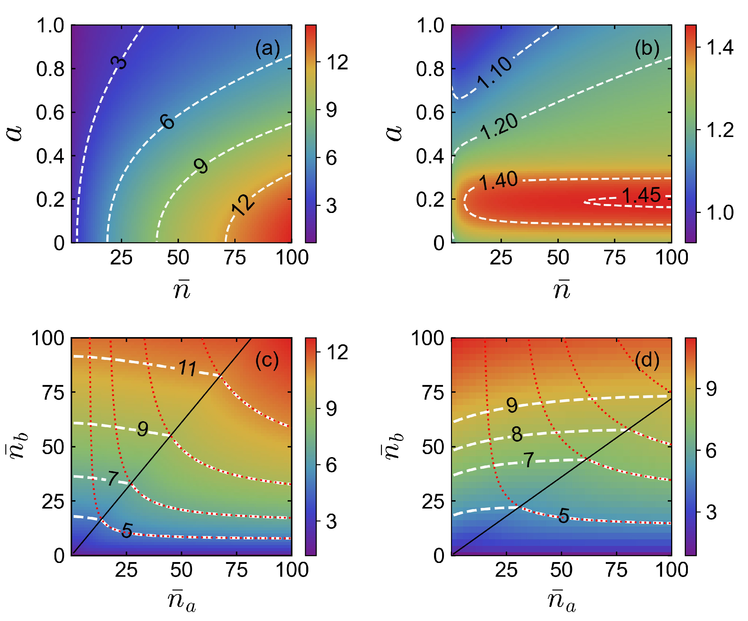
In Figure 2a,b, we show density plot of the ratios $\frac{2\pi /3}{\mathrm{FWHM}}$ and $\frac{1/\sqrt{\overline{n}}}{\delta {\theta }_{\mathrm{CRB},min}}$ as functions of the average photon number $\overline{n}$ and the bin size a, where $\delta {\theta }_{\mathrm{CRB},min}=1/\sqrt{\mathcal{F}({\theta }_{min})}$. Using the parameters similar to Schäfermeier et al. [10], one can find that the resolution is optimal as $a\to 0$, while the best sensitivity appears at $a\sim 0.183$, as predicted by Equation (22). Next, in Figure 2c,d, we show the validity of Equations (22) and (23) by calculating the ratio $\frac{1/\sqrt{\overline{n}}}{\delta {\theta }_{\mathrm{CRB},min}}$ against ${\overline{n}}_a$ and ${\overline{n}}_b$. For a pure squeezed vacuum with $\varrho =1$, one can find that contour lines of $\frac{1/\sqrt{\overline{n}}}{\delta {\theta }_{\mathrm{CRB},min}}$ (the white dashed lines) coincide with that of the analytic result $\frac{1/\sqrt{\overline{n}}}{\delta {\theta }_{\mathrm{CRB},\mathrm{ana}}}$ (the red dotted lines), as long as ${\overline{n}}_b/\overline{n}\lesssim 0.55$ (i.e., ${\overline{n}}_b\lesssim 1.2{\overline{n}}_a$). For the case $\varrho <1$, our analytic result can predict the best sensitivity, provided ${\overline{n}}_b/\overline{n}\lesssim 0.55\sqrt{\varrho }$ (e.g., ${\overline{n}}_b\lesssim 0.7{\overline{n}}_a$ for $\varrho =0.58$).

When ${\overline{n}}_b\gtrsim {\overline{n}}_a\gg 1$, our analytic result $\delta {\theta }_{\mathrm{CRB},\mathrm{ana}}$ shows a slight discrepancy with numerical result of the best sensitivity $\delta {\theta }_{\mathrm{CRB},min}$. However, it is still useful to predict the Heisenberg scaling of the sensitivity $\delta {\theta }_{\mathrm{CRB},\mathrm{ana}}\sim \mathcal{O}(1/\overline{n})$. One can see this by considering the limit ${\overline{n}}_b\gg 1$, for which $exp(2r)\approx 4{\overline{n}}_b$ (i.e., $e^{-r}\approx 1/\sqrt{4{\overline{n}}_b}$). If we set ${\overline{n}}_b/\overline{n}=\gamma$ (i.e., ${\overline{n}}_b=\gamma \overline{n}$), then Equation (23) reduces to

$$\delta {\theta }_{\mathrm{CRB},\mathrm{ana}}\approx \frac{1.11}{2\sqrt{\varrho {\overline{n}}_b{\overline{n}}_a}}=\frac{1.11}{2\sqrt{\gamma (1-\gamma )\varrho }}\frac{1}{\overline{n}}.$$

(24)

Similar to Ref. [21], let us consider the case ${\overline{n}}_a={\overline{n}}_b=\overline{n}/2$ (i.e., $\gamma =1/2$), which yields the sensitivity $\delta {\theta }_{\mathrm{CRB},\mathrm{ana}}\approx 1.11/(\overline{n}\sqrt{\varrho })$, coincident with the numerical result (see below).

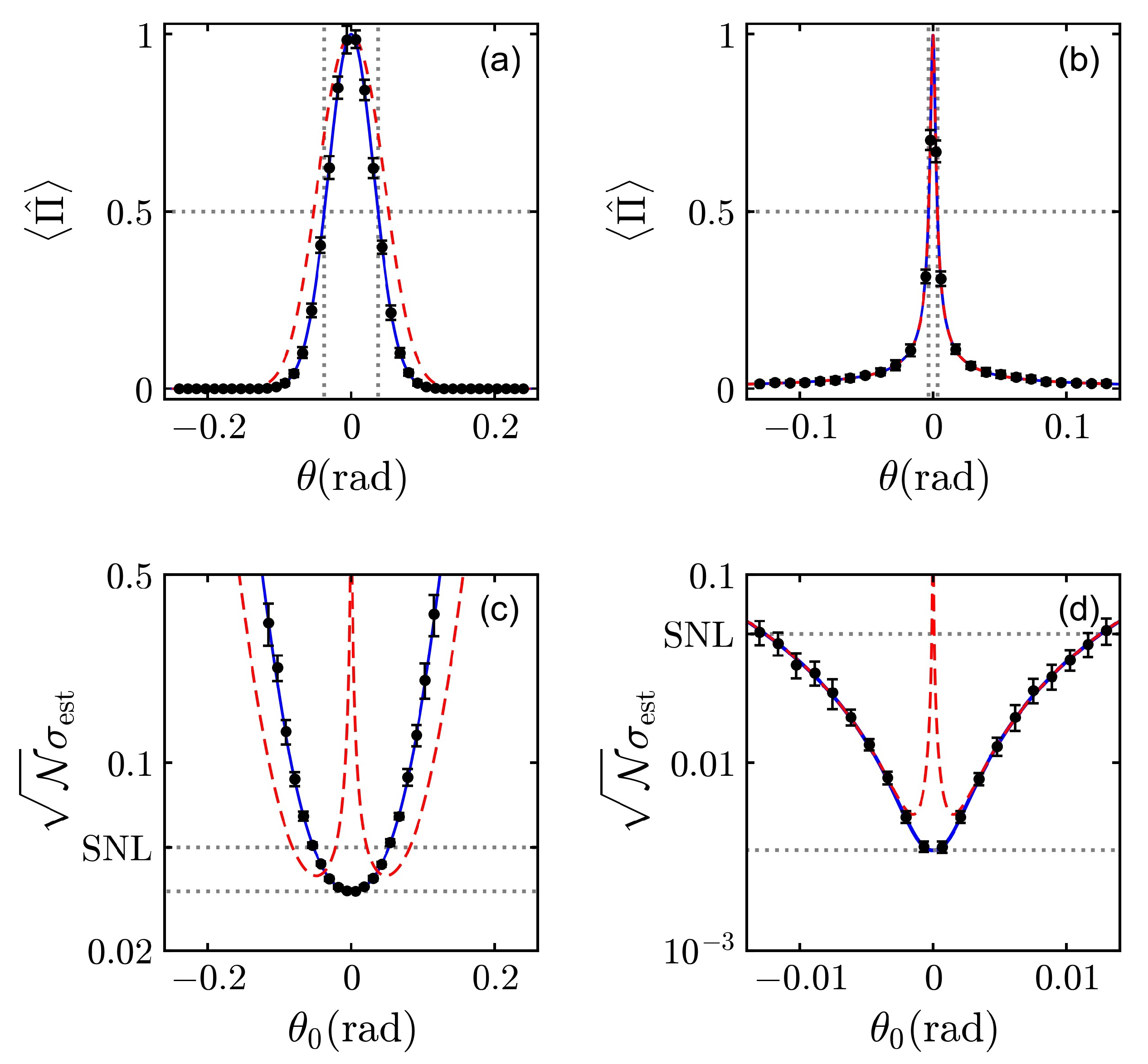
To confirm the above results, we show the signal and the sensitivity in Figure 3. In the left panel, we consider the squeezed vacuum with ${\overline{n}}_b\ll {\overline{n}}_a$ and the purity $\varrho =0.58$. One can see that both the resolution and the achievable sensitivity are better than that of the previous work [10], provided that an optimal value of a predicted by Equation (22) is adopted. In the right panel, we consider the case ${\overline{n}}_b={\overline{n}}_a=\overline{n}/2$ and compare our results with that of Schäfermeier et al. [10] using the same value of a. From Figure 3b, one can find that the signal and its resolution are the same with the binary–outcome case since we have taken the eigenvalues ${\mu }_{\pm }=0$ and ${\mu }_0=1/\mathrm{erf}(\sqrt{2\tilde{\nu }}a)$, similar to Schäfermeier et al. [10]. Remarkably, the solid line of Figure 3d indicates that the best sensitivity can reach the Heisenberg scaling $1.11/(\overline{n}\sqrt{\varrho })$, as predicted by Equation (24).

3. Approximate Maximum Likelihood Estimation

Finally, there remains a question how to saturate the CRB of the three–outcome measurement. Usually, the estimator by inverting the averaged signal cannot saturate the CRB, except for the case ${\mu }_{-}=+1$, ${\mu }_{+}=-1$, and ${\mu }_0=0$ (not shown here). It is therefore important to find out an optimal phase-estimation protocol, which can saturate the CRB. According to Ref. [39], the phase-estimation protocol consists of two steps. The first one is the calibration of the interferometer to obtain $\left\{P_k(\theta )\right\}$ by measuring the occurrence frequency $\{{\mathcal{N}}_k/\mathcal{N}\}$ at each given value of phase shift $\theta \in (-\pi ,\pi )$. Using ${\mu }_{\pm }=0$ and ${\mu }_0=1/\mathrm{erf}(\sqrt{2\varrho }a{e}^r)$ in Equation (12), one can obtain the signal within a single run of the calibration. After multiple runs, one can obtain statistical average of the signal and its standard deviation, as depicted by the circles and the bars in Figure 3a,b.

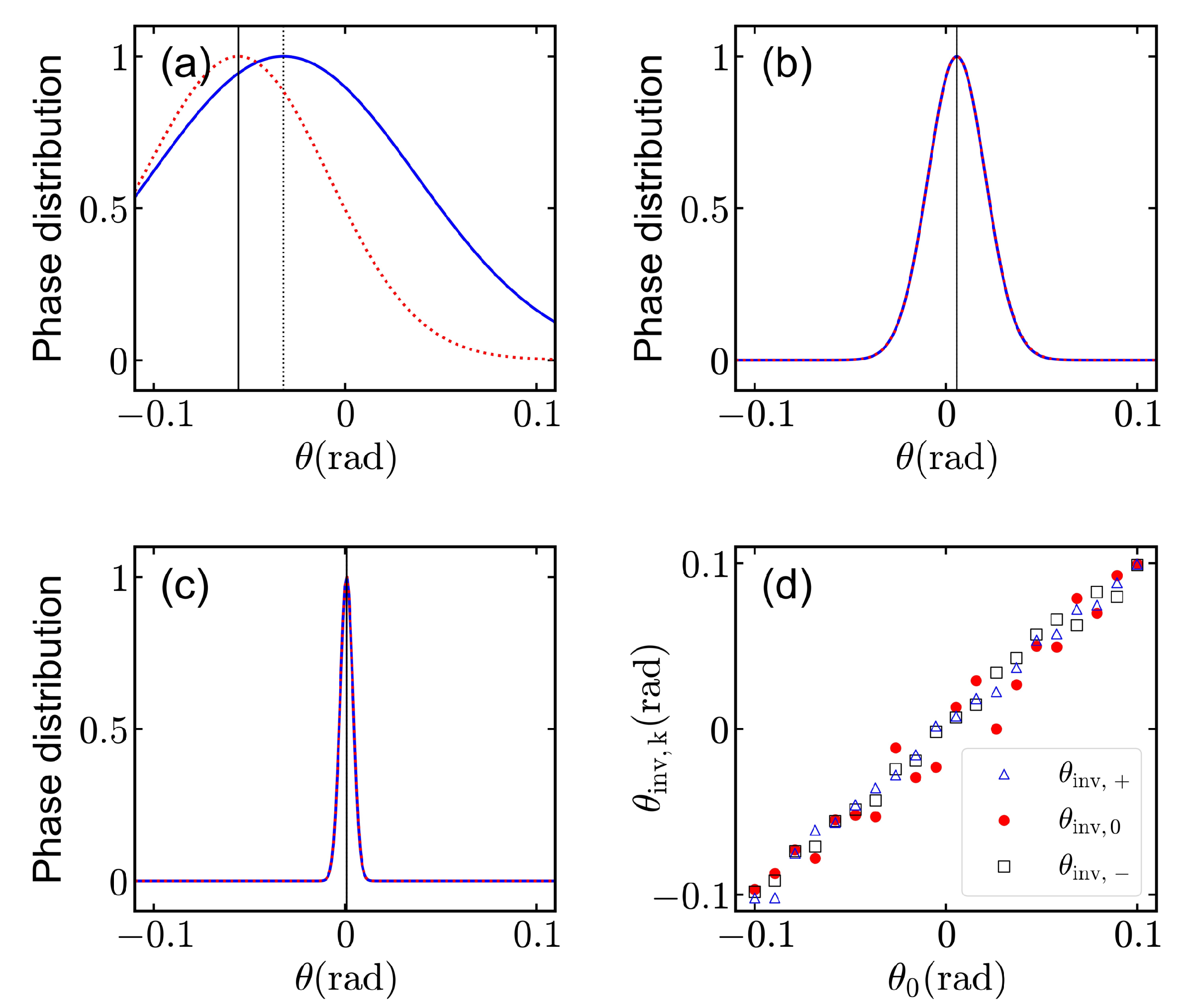
After the calibration, we can perform maximum Likelihood estimation, since the estimator adopted (i.e., the MLE) is well known asymptotically optimal (see, e.g., Ref. [13]). As shown by the red dotted lines of Figure 4a–c, the MLE can be determined by the peak of the likelihood function (which is simply a multinomial distribution):

$$\mathcal{P}(\theta |\left\{{\mathcal{N}}_k\right\})=\mathcal{N}!\prod _k\frac{1}{{\mathcal{N}}_k!}{\left[P_k(\theta )\right]}^{{\mathcal{N}}_k},$$

(25)

where ${\mathcal{N}}_k={\mathcal{N}}_k({\theta }_0)$ denotes the occurrence number of each outcome at a given true value of phase shift ${\theta }_0$. When ${\mathcal{N}}_k\sim \mathcal{O}(\mathcal{N})$ and $\mathcal{N}={\sum }_k{\mathcal{N}}_k\gg 1$, the phase distribution can be approximated as a Gaussian (see the solid lines of Figure 4a–c, and also Ref. [20])

$$\mathcal{P}(\theta |\left\{{\mathcal{N}}_k\right\})\propto exp\left[-\frac{1}{2{\sigma }_{\mathrm{est}}^2}{\left(\theta -{\theta }_{\mathrm{est}}\right)}^2\right],$$

(26)

where we have introduced

$${\theta }_{\mathrm{est}}=\sum _k{c}_k{\theta }_{\mathrm{inv},k},c_k=\frac{f_k\left({\theta }_{\mathrm{inv},k}\right)}{{\sum }_{k^{\prime }}{f}_{k^{\prime }}\left({\theta }_{\mathrm{inv},k^{\prime }}\right)},$$

(27)

and

$${\sigma }_{\mathrm{est}}=\frac{1}{\sqrt{\mathcal{N}{\sum }_k{f}_k({\theta }_{\mathrm{inv},k})}},$$

(28)

with the inversion estimator associated with the k-th outcome ${\theta }_{\mathrm{inv},k}=P_k^{-1}({\mathcal{N}}_k/\mathcal{N})$ and the CFI $f_k(\theta )={\left[P_k^{\prime }(\theta )\right]}^2/P_k(\theta )$. The estimator ${\theta }_{\mathrm{est}}$ shows clear physical meaning as a linear combination of all the inversion estimators, weighted by the CFI of each outcome. When the CFI of the outcome $k=0$ dominates over that of the others, then Equation (27) simply reduces to ${\theta }_{\mathrm{est}}\approx {\theta }_{\mathrm{inv},0}$. Furthermore, ${\sigma }_{\mathrm{est}}$ is a $68.3\%$ confidence interval of the Gaussian around ${\theta }_{\mathrm{est}}$, similar to the MLE [21,38].

To obtain ${\theta }_{\mathrm{est}}$, it requires to measure all the probabilities $\left\{P_k(\theta )\right\}$ and hence $\left\{f_k(\theta )\right\}$, as well as the inversion estimators $\left\{{\theta }_{\mathrm{inv},k}\right\}$. For each outcome, one has to solve a unique root of the equation $P_k(\theta )={\mathcal{N}}_k/\mathcal{N}$ around ${\theta }_0$. This requires some prior information about the true value of phase shift. When the prior knowledge is not sufficient, one can use multi-step estimation protocol [40,41,42], or simply a two-step protocol [43]. As shown by Figure 4d, one can see the inversion estimators of all the outcomes ${\theta }_{\mathrm{inv},k}\approx {\theta }_0$ and hence $\mathcal{F}({\theta }_0)\approx {\sum }_k{f}_k({\theta }_{\mathrm{inv},k})$, which in turn results in ${\sigma }_{\mathrm{est}}\approx 1/\sqrt{\mathcal{NF}({\theta }_0)}$. This means that the estimator ${\theta }_{\mathrm{est}}$ can saturate the CRB for a multi-outcome detection with large enough $\mathcal{N}$. Indeed, Equations (25)–(28) are valid for arbitrary kinds of multi-outcome detection [20]. In Figure 3c,d, we numerically show this result for the three-outcome homodyne detection, using M replicas of $\mathcal{N}$ ($={10}^3$) random numbers at each given ${\theta }_0$. One can see that statistical averages of $\{{\sigma }_{\mathrm{est}}^{(1)}$, ${\sigma }_{\mathrm{est}}^{(2)}$, $...$, ${\sigma }_{\mathrm{est}}^{(M)}\}$ (the circles) almost saturate the CRB (the blue solid line).

4. Discussion and Conclusions

From Figure 1c, one can see that the signal shows a better resolution than that of the binary–outcome measurement scheme [10], provided that a relatively small value of a is adopted. However, it results in a reduced sensitivity; see the solid line of Figure 1d. Such a problem can be bypassed using the CRB of a three-outcome measurement; see the red dotted line of Figure 1d. By maximizing the CFI, we derived analytic results of the best sensitivity and the associated optimal value of a. Our analytic results start from the condition ${\overline{n}}_b\ll {\overline{n}}_a$. Numerically, we show that this condition can be relaxed to ${\overline{n}}_b\lesssim 0.7{\overline{n}}_a$ for the purity $\varrho =0.58$. For the case ${\overline{n}}_b\gtrsim {\overline{n}}_a\gg 1$, our analytic results may also be of importance to predict the Heisenberg scaling of the sensitivity; see Equation (24) and also Figure 3d. Finally, we present an optimal phase estimator by approximating the multinomial phase distribution of a multi-outcome measurement by a Gaussian and show the underlying physics of why the MLE can saturate the CRB.

In summary, we have investigated high-precision homodyne measurement and data processing at a single output port of the interferometer fed by a coherent state and a squeezed vacuum of light, where the measurement quadrature is divided into three bins. As a three-outcome measurement, this kind of data processing can further improve the phase resolution and the phase sensitivity beyond the binary–outcome case. By maximizing the Fisher information, we obtain the optimal value of the bin size and the best sensitivity, i.e., Equations (22) and (23). Our analytical results show good agreement with the exact numerical results and are useful to predict the Heisenberg scaling of the sensitivity. Finally, we show an approximate maximum-likelihood estimation with respect to the three-outcome homodyne detections. Our numerical simulations indicate that the phase estimator can saturate the Cramér–Rao lower bound of the sensitivity and hence is asymptotically optimal.

References

- The LIGO Scientific Collaboration. A gravitational wave observatory operating beyond the quantum shot-noise limit. Nat. Phys. 2011, 7, 962. [Google Scholar] [CrossRef] [Green Version]
- The LIGO Scientific Collaboration. Enhanced sensitivity of the LIGO gravitational wave detector by using squeezed states of light. Nat. Photonics 2013, 7, 613. [Google Scholar] [CrossRef]
- Taylor, M.A.; Bowen, W.P. Quantum metrology and its application in biology. Phys. Rep. 2016, 615, 1–59. [Google Scholar] [CrossRef] [Green Version]
- Mauranyapin, N.; Madsen, L.; Taylor, M.; Waleed, M.; Bowen, W. Evanescent single-molecule biosensing with quantum-limited precision. Nat. Photonics 2017, 11, 477. [Google Scholar] [CrossRef]
- Ludlow, A.D.; Boyd, M.M.; Ye, J.; Peik, E.; Schmidt, P.O. Optical atomic clocks. Rev. Mod. Phys. 2015, 87, 637. [Google Scholar] [CrossRef]
- Katori, H. Optical lattice clocks and quantum metrology. Nat. Photonics 2011, 5, 203. [Google Scholar] [CrossRef]
- Jones, J.A.; Karlen, S.D.; Fitzsimons, J.; Ardavan, A.; Benjamin, S.C.; Briggs, G.A.D.; Morton, J.J.L. Magnetic field sensing beyond the standard quantum limit using 10-spin noon states. Science 2009, 324, 1166–1168. [Google Scholar] [CrossRef] [PubMed] [Green Version]
- Boto, A.N.; Kok, P.; Abrams, D.S.; Braunstein, S.L.; Williams, C.P.; Dowling, J.P. Quantum Interferometric Optical Lithography: Exploiting Entanglement to Beat the Diffraction Limit. Phys. Rev. Lett. 2000, 85, 2733. [Google Scholar] [CrossRef]
- Caves, C.M. Quantum-mechanical noise in an interferometer. Phys. Rev. D 1981, 23, 1693. [Google Scholar] [CrossRef]
- Schäfermeier, C.; Ježek, M.; Madsen, L.S.; Gehring, T.; Andersen, U.L. Deterministic phase measurements exhibiting super-sensitivity and super-resolution. Optica 2018, 5, 60–64. [Google Scholar] [CrossRef] [Green Version]
- Distante, E.; Ježek, M.; Andersen, U.L. Deterministic Superresolution with Coherent States at the Shot Noise Limit. Phys. Rev. Lett. 2013, 111, 033603. [Google Scholar] [CrossRef] [PubMed] [Green Version]
- Yurke, B.; McCall, S.L.; Klauder, J.R. SU(2) and SU(1,1) interferometers. Phys. Rev. A 1986, 33, 4033. [Google Scholar] [CrossRef] [PubMed]
- Helstrom, C.W. Quantum Detection and Estimation Theory; Academic: New York, NY, USA, 1976. [Google Scholar]
- Holevo, A.S. Probabilistic and Statistical Aspects of Quantum Theory; North-Holland Publishing Company: Amsterdam, The Netherlands, 1982. [Google Scholar]
- Giovannetti, V.; Lloyd, S.; Maccone, L. Quantum-Enhanced Measurements: Beating the Standard Quantum Limit. Science 2004, 306, 1330. [Google Scholar] [CrossRef] [PubMed] [Green Version]
- Giovannetti, V.; Lloyd, S.; Maccone, L. Advances in quantum metrology. Nat. Photonics 2011, 5, 222–229. [Google Scholar] [CrossRef]
- Braunstein, S.L.; Caves, C.M. Statistical distance and the geometry of quantum states. Phys. Rev. Lett. 1994, 72, 3439–3440. [Google Scholar] [CrossRef]
- Braunstein, S.L.; Caves, C.M.; Milburn, G.J. Generalized uncertainty relations: Theory, examples, and Lorentz invariance. Ann. Phys. 1996, 247, 135. [Google Scholar] [CrossRef] [Green Version]
- Paris, M.G.A. Quantum estimation for quantum technology. In. J. Quantum Inform. 2009, 7, 125. [Google Scholar] [CrossRef]
- Zhou, L.K.; Xu, J.H.; Zhang, W.-Z.; Cheng, J.; Yin, T.S.; Yu, Y.B.; Chen, R.P.; Chen, A.X.; Jin, G.R.; Yang, W. Linear combination estimator of multiple-outcome detections with discrete measurement outcomes. Phys. Rev. A 2021, 103, 043702. [Google Scholar] [CrossRef]
- Pezzé, L.; Smerzi, A. Mach-Zehnder Interferometry at the Heisenberg Limit with Coherent and Squeezed-Vacuum Light. Phys. Rev. Lett. 2008, 100, 073601. [Google Scholar] [CrossRef] [Green Version]
- Liu, P.; Wang, P.; Yang, W.; Jin, G.R.; Sun, C.P. Fisher information of a squeezed-state interferometer with a finite photon-number resolution. Phys. Rev. A 2017, 95, 023824. [Google Scholar] [CrossRef] [Green Version]
- Liu, P.; Jin, G.R. Ultimate phase estimation in a squeezed-state interferometer using photon counters with a finite number resolution. J. Phys. A Math. Theor. 2017, 50, 405303. [Google Scholar] [CrossRef] [Green Version]
- Gerry, C.C.; Knight, P.L. Introductory Quantum Optics; Cambridge University: Cambridge, UK, 2005. [Google Scholar]
- Seshadreesan, K.P.; Anisimov, P.M.; Lee, H.; Dowling, J.P. Parity detection achieves the Heisenberg limit in interferometry with coherent mixed with squeezed vacuum light. New J. Phys. 2011, 13, 083026. [Google Scholar] [CrossRef]
- Tan, Q.S.; Liao, J.Q.; Wang, X.G.; Nori, F. Enhanced interferometry using squeezed thermal states and even or odd states. Phys. Rev. A 2014, 89, 053822. [Google Scholar] [CrossRef] [Green Version]
- Wang, J.Z.; Yang, Z.Q.; Chen, A.X.; Yang, W.; Jin, G.R. Multi-outcome homodyne detection in a coherent-state light interferometer. Opt. Express 2019, 27, 10343. [Google Scholar] [CrossRef] [Green Version]
- Xu, J.H.; Chen, A.X.; Yang, W.; Jin, G.R. Data processing over single-port homodyne detection to realize superresolution and supersensitivity. Phys. Rev. A 2019, 100, 063839. [Google Scholar] [CrossRef] [Green Version]
- Bollinger, J.J.; Itano, W.M.; Wineland, D.J.; Heinzen, D.J. Optimal frequency measurements with maximally correlated states. Phys. Rev. A 1996, 54, R4649. [Google Scholar] [CrossRef] [Green Version]
- Gerry, C.C.; Campos, R.A.; Benmoussa, A. Comment on Interferometric Detection of Optical Phase Shifts at the Heisenberg Limit. Phys. Rev. Lett. 2004, 92, 209301. [Google Scholar] [CrossRef]
- Gerry, C.C. Heisenberg-limit interferometry with four-wave mixers operating in a nonlinear regime. Phys. Rev. A 2000, 61, 043811. [Google Scholar] [CrossRef]
- Gerry, C.C.; Benmoussa, A.; Campos, R.A. Nonlinear interferometer as a resource for maximally entangled photonic states: Application to interferometry. Phys. Rev. A 2002, 66, 013804. [Google Scholar] [CrossRef]
- Gao, Y.; Anisimov, P.M.; Wildfeuer, C.F.; Luine, J.; Lee, H.; Dowling, J.P. Super-resolution at the shot-noise limit with coherent states and photon-number-resolving detectors. J. Opt. Soc. Am. B 2010, 27, A170–A174. [Google Scholar] [CrossRef] [Green Version]
- Feng, X.M.; Jin, G.R.; Yang, W. Quantum interferometry with binary–outcome measurements in the presence of phase diffusion. Phys. Rev. A 2014, 90, 013807. [Google Scholar] [CrossRef] [Green Version]
- Xiang, G.Y.; Hofmann, H.F.; Pryde, G.J. Optimal multi-photon phase sensing with a single interference fringe. Sci. Rep. 2013, 3, 2684. [Google Scholar] [CrossRef] [Green Version]
- Cohen, L.; Istrati, D.; Dovrat, L.; Eisenberg, H.S. Super-resolved phase measurements at the shot noise limit by parity measurement. Opt. Express 2014, 22, 11945–11953. [Google Scholar] [CrossRef]
- Israel, Y.; Rosen, S.; Silberberg, Y. Supersensitive Polarization Microscopy Using NOON States of Light. Phys. Rev. Lett. 2014, 112, 103604. [Google Scholar] [CrossRef]
- Jin, G.R.; Yang, W.; Sun, C.P. Quantum-enhanced microscopy with binary–outcome photon counting. Phys. Rev. A 2017, 95, 013835. [Google Scholar] [CrossRef] [Green Version]
- Pezzé, L.; Smerzi, A.; Khoury, G.; Hodelin, J.F.; Bouwmeester, D. Phase detection at the quantum limit with multiphoton Mach-Zehnder interferometry. Phys. Rev. Lett. 2007, 99, 223602. [Google Scholar] [CrossRef] [PubMed] [Green Version]
- Pezzé, L.; Smerzi, A. Sub shot-noise interferometric phase sensitivity with beryllium ions Schrödinger cat states. Europhys. Lett. 2007, 78, 30004. [Google Scholar] [CrossRef]
- Higgins, B.L.; Berry, D.W.; Bartlett, S.D.; Wiseman, H.M.; Pryde, G.J. Entanglement-free Heisenberg-limited phase estimation. Nature 2007, 450, 393. [Google Scholar] [CrossRef] [PubMed] [Green Version]
- Berry, D.W.; Higgins, B.L.; Bartlett, S.D.; Mitchell, M.W.; Pryde, G.J.; Wiseman, H.M. How to perform the most accurate possible phase measurements. Phys. Rev. A 2009, 80, 052114. [Google Scholar] [CrossRef] [Green Version]
- Hayashi, M.; Vinjanampathy, S.; Kwek, L.C. Resolving unattainable Cramer-Rao bounds for quantum sensors. J. Phys. B At. Mol. Opt. Phys. 2019, 52, 015503. [Google Scholar] [CrossRef]
Figure 1.
(a) Homodyne detection at one port of the interferometer fed by a coherent state and a squeezed vacuum , equivalent to the field quadrature measurement; (b) 3D plot of the measurement probability given by Equation (6); (c,d) the output signal and the phase sensitivity for (solid) and (dashed), obtained by taking and in Equations (12) or (14). The red dotted line in (d) is the CRB for the three-outcome measurement for . Vertical lines in (c) the of the signal. Horizontal lines in (d) the upper one corresponds to the SNL and the other is given by Equation (23). Other paraments: , (i.e., ), and , similar to Ref. [10].
Figure 2.
(a,b) Density plots of the ratios and as functions of the average photon number and the bin size a, with the parameters and [10]; (c,d) density plot of the ratio against and for (c) and (d). Red dotted lines: analytic result of Equation (23), coincident with the numerical result below the solid lines that determined by .
Figure 3.
Numerical simulations of the signal (a,b) and the sensitivity (c,d) for (a,c) and (b,d) with , using (a,c) and (b,d), as predicted by Equation (22). The circles and the bars: statistical average of the signal and the error per measurement (i.e., ) and their associated standard deviations, simulated with 20 replicas of random numbers at each given phase shift. Red dashed lines: the signal and the sensitivity of the binary–outcome measurement for (a,c) and (b,d). Horizontal lines in (c,d) the upper lines correspond to the SNL , and the other is given by Equation (23) and , respectively. All for the purity .
Figure 4.
Given the true value of the phase shift , phase distribution (red dashed) and its approximate result (solid) as a function of , simulated with random numbers for (a) , (b) , (c) . (d) The inversion estimators of the three-outcome homodyne detection for different values of . Parameters: and the others the same with Figure 1c,d.
Publisher’s Note: MDPI stays neutral with regard to jurisdictional claims in published maps and institutional affiliations. |
© 2021 by the authors. Licensee MDPI, Basel, Switzerland. This article is an open access article distributed under the terms and conditions of the Creative Commons Attribution (CC BY) license (https://creativecommons.org/licenses/by/4.0/).
Share and Cite
MDPI and ACS Style
Zhou, L.; Liu, P.; Jin, G.-R. Single-Port Homodyne Detection in a Squeezed-State Interferometry with Optimal Data Processing. Photonics 2021, 8, 291. https://0-doi-org.brum.beds.ac.uk/10.3390/photonics8080291
AMA Style
Zhou L, Liu P, Jin G-R. Single-Port Homodyne Detection in a Squeezed-State Interferometry with Optimal Data Processing. Photonics. 2021; 8(8):291. https://0-doi-org.brum.beds.ac.uk/10.3390/photonics8080291
Chicago/Turabian StyleZhou, Likun, Pan Liu, and Guang-Ri Jin. 2021. "Single-Port Homodyne Detection in a Squeezed-State Interferometry with Optimal Data Processing" Photonics 8, no. 8: 291. https://0-doi-org.brum.beds.ac.uk/10.3390/photonics8080291
Note that from the first issue of 2016, this journal uses article numbers instead of page numbers. See further details here.