Solvent and Substituent Effects on the Phosphine + CO2 Reaction


1
Instituto de Química Médica, CSIC, Juan de la Cierva, 3, E-28006 Madrid, Spain
2
Trinity Biomedical Sciences Institute, School of Chemistry, The University of Dublin, Trinity College, Dublin 2, Ireland
3
Irish Centre of High-End Computing, Grand Canal Quay, Dublin 2, Ireland
*
Authors to whom correspondence should be addressed.
Inorganics 2018, 6(4), 110; https://0-doi-org.brum.beds.ac.uk/10.3390/inorganics6040110
Submission received: 25 September 2018
/
Revised: 1 October 2018
/
Accepted: 3 October 2018
/
Published: 10 October 2018
(This article belongs to the Special Issue Novel Non-Covalent Interactions)
Abstract
:A theoretical study of the substituent and solvent effects on the reaction of phosphines with CO2 has been carried out by means of Møller-Plesset (MP2) computational level calculations and continuum polarizable method (PCM) solvent models. Three stationary points along the reaction coordinate have been characterized, a pre-transition state (TS) assembly in which a pnicogen bond or tetrel bond is established between the phosphine and the CO2 molecule, followed by a transition state, and leading finally to the adduct in which the P–C bond has been formed. The solvent effects on the stability and geometry of the stationary points are different. Thus, the pnicogen bonded complexes are destabilized as the dielectric constant of the solvent increases while the opposite happens within the adducts with the P–C bond and the TSs trend. A combination of the substituents and solvents can be used to control the most stable minimum.
1. Introduction
In the field of weak interactions, the initial level of the calculations was devoted to complexes formed by two molecules, A and B, of complementary properties, e.g., an electron donor and an electron acceptor. The next step were studies concerning the effect of a third molecule, C, that through a weak interaction with A (or B) modifies the first complex properties. Since A, B, and C can be the same molecule, these A···A···A trimers are the start of clusters, An. Since the interaction of small molecules, such as drugs, with proteins involve the perturbation of the weak interactions present in proteins by a third molecule acting also by weak interactions, these studies are of paramount importance.
In the field of solvent effects there are specific and bulky effects. The specific effects are due to weak interactions, mainly hydrogen bonds, which are theoretically studied building up supramolecules, for instance, proton transfer in pyrazoles being assisted by two linked water molecules [1,2,3]. The general solvent effects consider the solvent as bulk and are studied empirically using solvent scales (Kamlet et al. [4], Reichardt [5], Abraham [6], Catalán [7]), as well as theoretically using the polarizable continuum model, PCM (Tomasi et al. [8]), the conductor-like screening model, COSMO (Orozco and Luque [9]), and Density Functional Solvation Model, DGSOL (Zhu et al. [10]). Note that several authors have studied solvent effects on weak interactions using the PCM approximation [11,12,13,14,15,16].
Concerning the carbon dioxide greenhouse effect, after some previous attempts by scientists like John Tyndall, Svante Arrhenius, Guy Stewart Callendar and others, it was Charles David Keeling in the early 1960s that established definitely that CO2 produces a greenhouse effect [17,18,19,20,21,22,23,24]. There are numerous studies related with CO2 including in catalysis [25], processing polymers [26], engineering [27], absorption processes [28,29], crop development [30], fuels [31], lasers [32], and combustion research [33]. Also, the CO2 molecule has been the subject of investigation from the theoretical point of view [29,34,35]. Our previous studies concerning A···B complexes with B being CO2 are reported in references [36,37,38,39,40,41].
Simulation of phosphorous/boron frustrated lewis pair complexes (FLP) with CO2 in explicit solvent proposed a two-step mechanism [42]. The effect of the solvent has been considered on the carbene + CO2 reaction [43,44] and in the anion + CO2 one [45].
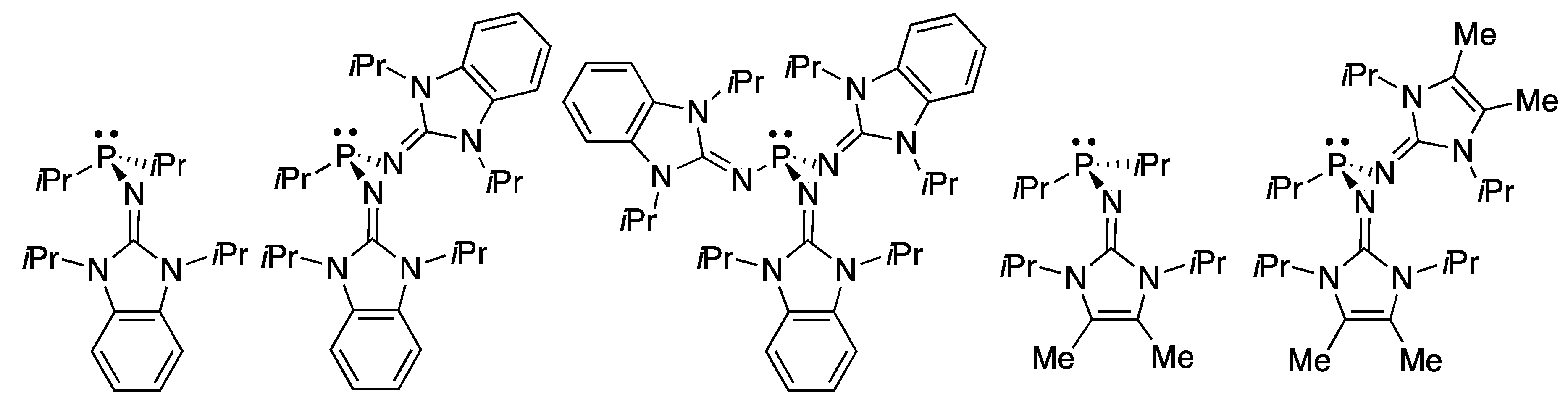
Dielman et al. reported the interaction of phosphines with CO2 [46,47]. Among the reversible CO2 binding by zwitterionic Lewis base adducts (cyclic guanidines, N-heterocyclic carbenes, NHCs) the authors describe the behavior of electron-rich phosphines (Figure 1) [46]. The ability of these compounds to form adducts with CO2 has been rationalized based on the Tolman electronic parameter [48].
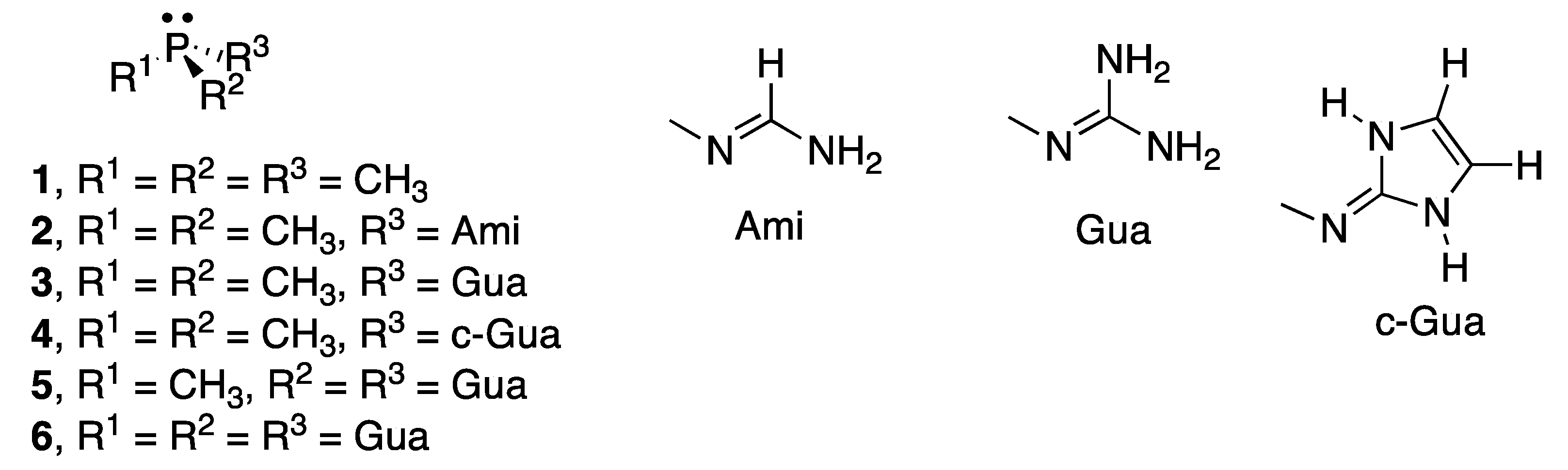
In this article, we have carried out a computational study of the reaction of six phosphines (Figure 2) with CO2 to form the corresponding phosphine-CO2 adducts in the gas phase and in eight solvents of increasing polarity (hexane, toluene, chloroform, 1-octanol, acetone, dimethylsulfoxide, water, and formamide). Three stationary points in the energy profile have been characterized, two of them are energetic minimum which corresponds to the non-covalent complexes between the phosphine and CO2, and to the adduct with a P–C bond. In addition, the transition states linking both minima have been located. The effect of the substituents on the reaction has been considered by replacing one of the methyl groups of trimethylphosphine by amidine and by two different guanidines. In addition, the phosphines bonded to two and three guanidine groups have been examined.
2. Results
In this section, the nomenclature used within the article will be briefly outlined, followed by an in-depth discussion of the stationary points within the 1 + CO2 energy profile, and finally the rest of the cases—2 to 6 (Figure 2)—will be discussed.
In order to differentiate the three stationary structures characterized within the manuscript, the “:”, “-“, and “/” symbols between the phosphine and the CO2 molecule will be used to indicate the complex, adduct, and transition structure, respectively. Thus, 1:CO2, 1-CO2, and 1/CO2 will correspond to the three stationary points in the 1 + CO2 energy profile (complex, adduct, and transition state (TS), respectively).
2.1. (CH3)3P + CO2 (1)
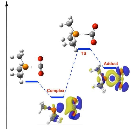
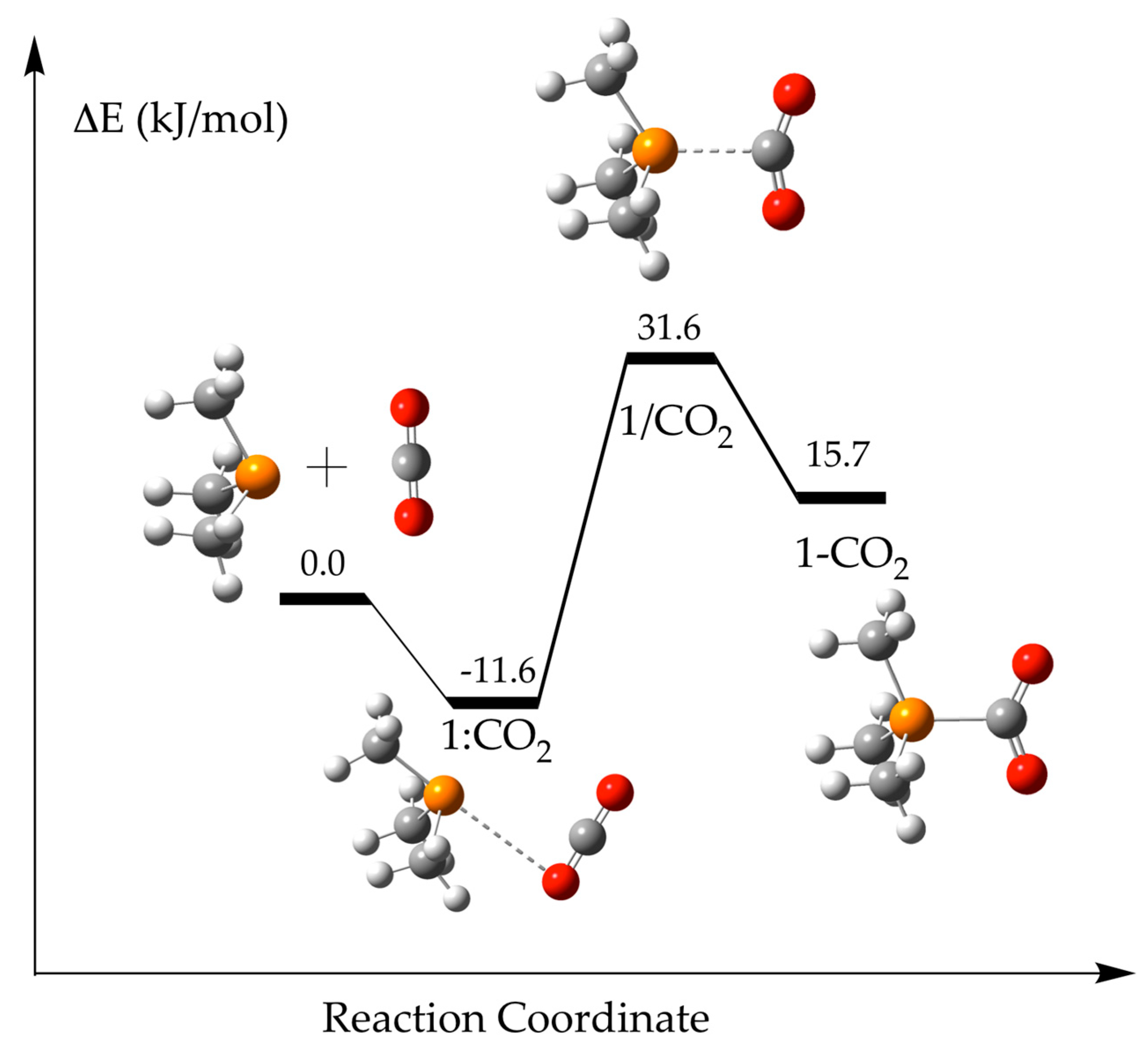
The reference phosphine molecule [(CH3)3P, 1] shows only one stationary point in its reaction with CO2 in gas phase. It corresponds to the non-covalent pnicogen complex [49,50,51] with one of the oxygen atoms of the CO2 acting as an electron donor towards one of the σ-holes of the phosphine [1:CO2]. All attempts to obtain the adduct compound with a P–C bond evolves towards the non-covalent complex spontaneously. However, with the inclusion of the solvent effect, both minima, pnicogen complex, and adduct, are obtained and the corresponding TS were located (see Figure 3 for the stationary points with chloroform as solvent). The binding energy (Eb) of the 1:CO2 complex decreases uniformly from −14.5 kJ·mol−1 in gas phase to −10.6 in formamide as the dielectric constant of the solvent increases (Table 1). In contrast, the opposite trend is observed for the relative energy of the adduct in which the P–C bond is present vs. the isolated phosphine plus CO2. The 1-CO2 adduct in hexane shows the largest positive binding energy of 34.2 kJ·mol−1 as an indication that this structure is less stable than the isolated monomers. This is also observed for other solvents (toluene, chloroform, 1-octanol, and acetone) while in the most polar solvents (DMSO, water, and formamide), the relative energy is negative as an indication that the structure is more stable than the isolated molecules (−0.4, −1.3, and −1.6 kJ·mol−1, respectively). However, since the non-covalent complex, 1:CO2, is always more stable than the adduct one, it is expected that the population of the last one should be very small.
The relative energy of the TS that connects both minima also decreases as the dielectric constant of the solvent increases from 38.5 kJ·mol−1 in hexane to 28.1 kJ·mol−1 in formamide. Linear correlations between the energetic values (Eb) of each stationary point and the inverse of the dielectric constant of the solvent show good R2 correlations (R2 > 0.94, see Figure S1 of the Supplementary Materials). However, the curvature observed in the values indicates that a more complex relationship, like a second order polynomial, should provide a better fitting (R2 > 0.9999).
An inspection of the dipole moment of the different stationary points provides clues of the energetic trends upon solvation. The pnicogen bonded complex (1:CO2) shows small dipole moment ranging between 1.5 and 2.0 Debyes depending on the solvent considered. These values are similar to the dipole moment of the isolated phosphine (notice that the dipole moment of the isolated CO2 is 0.0 Debyes). In contrast, the dipole moment of the 1-CO2 adduct presents values between 10.0 and 12.4 Debyes which is much larger than the sum of the two isolated monomers. Thus, a larger stabilization of 1-CO2 due to solvation should be expected when compared to that of 1:CO2. The situation of the TS (1/CO2) is intermediate with a dipole moment that goes from 7.9 to 7.2 Debyes.
The intermolecular P···C and P···O distances in the complex increase as the dielectric constant of the solvent does. The P–C distance in the adduct decreases with the solvent polarity. These two effects are in accordance with the energetic variation observed due to the different solvents. In the case of the TSs, the intermolecular distance increases with the solvent in agreement with the Hammond postulate since the energy difference between the adduct and the complex decreases with the solvent polarity and the TS should tend to resemble more the complex.
The analysis of the electron density within the quantum theory of atoms in molecules (QTAIM) framework (Table S1) shows the presence of an intermolecular O···P bond critical point (BCP) in the 1:CO2 complex while it is a C···P BCP in the 1-CO2 adduct and 1/CO2 TS. The former shows the typical characteristic of a weak interaction: small value of the electron density at the bond critical point, ρBCP, (between 0.0087 and 0.077 au) and positive Laplacian values, ∇2ρBCP, (between 0.026 and 0.023 au) and total electron energy density, HBCP, approximately 0.001 au. In contrast, the P–C BCP in the adduct shows value characteristics of a polar bond with ρBCP between 0.156 and 0.145 au, ∇2ρBCP between −0.365 and −0.272 au, and HBCP between −0.143 and −0.100 au. The electron densities descriptors at the BCP in the TSs present values in between a covalent bond and a weak interaction. A more detailed analysis of the properties of the BCPs will be discussed later.
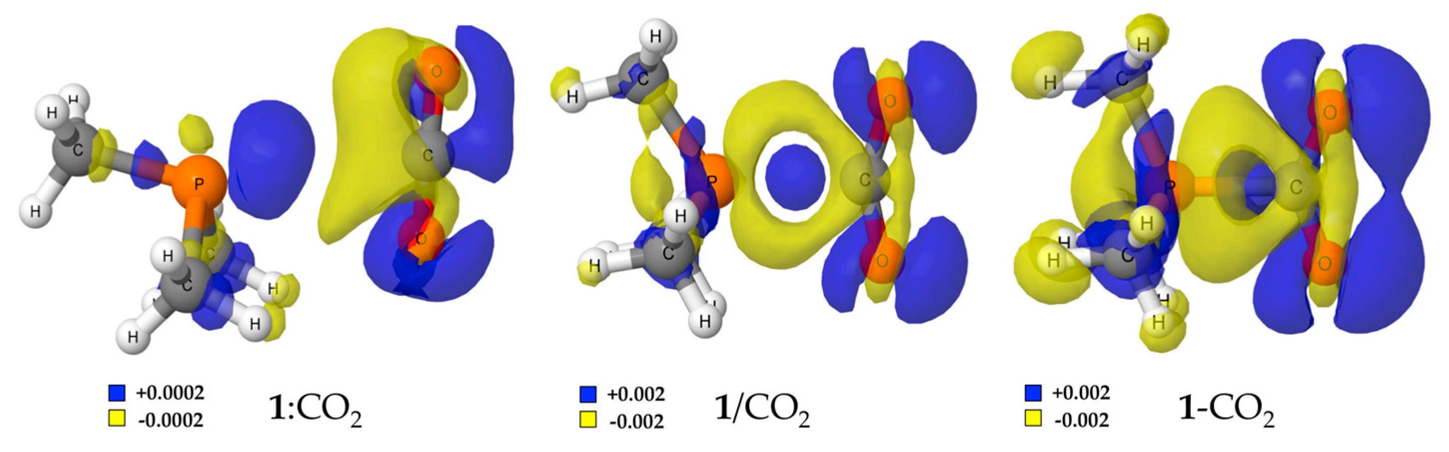
The electron density shift maps (obtained as difference of the electron density on the complex minus the electron density of the monomers in the geometry of the complex) [52] clearly show the polarization of the two interacting systems as the reaction process from the complex to the adduct is in good agreement with the dipole increment previously indicated. Please notice that the electron density shift (EDS) maps in Figure 4 for the complex are one order of magnitude smaller (±0.0002 au) than those of the TS and adduct (±0.002 au). Thus, a significant increment of charge (blue regions) is accumulated around the oxygen atoms of the CO2 in 1/CO2 adduct, mainly due to a loss of electron density on the hydrogens of the methyl groups of 1. In the region between P and C atoms, where the P–C bond is being formed, a loss of the electron density (yellow area) is shown within the area where the lone pair of the phosphorous was located, while an increase on the electron density (blue area) close to the carbon atom on the CO2 moiety is observed.
2.2. RR’R’’P + CO2 (2–5)
Once the smallest model of the reaction has been analysed the rest of the cases under study (2 to 6 in Figure 2) will be discussed. Three stationary points (complex, TS, and adduct) were found for all the rest of the systems considered in gas phase and regarding the solvent used, except for 3 + CO2 in gas phase where only the 3:CO2 complex with the pnicogen interaction was located. All the attempts to obtain 3-CO2 adduct in gas phase reverted spontaneously into the complex configuration. The binding energy of the stationary points in the different PCM models has been gathered in the Supplementary Material (Table S2).
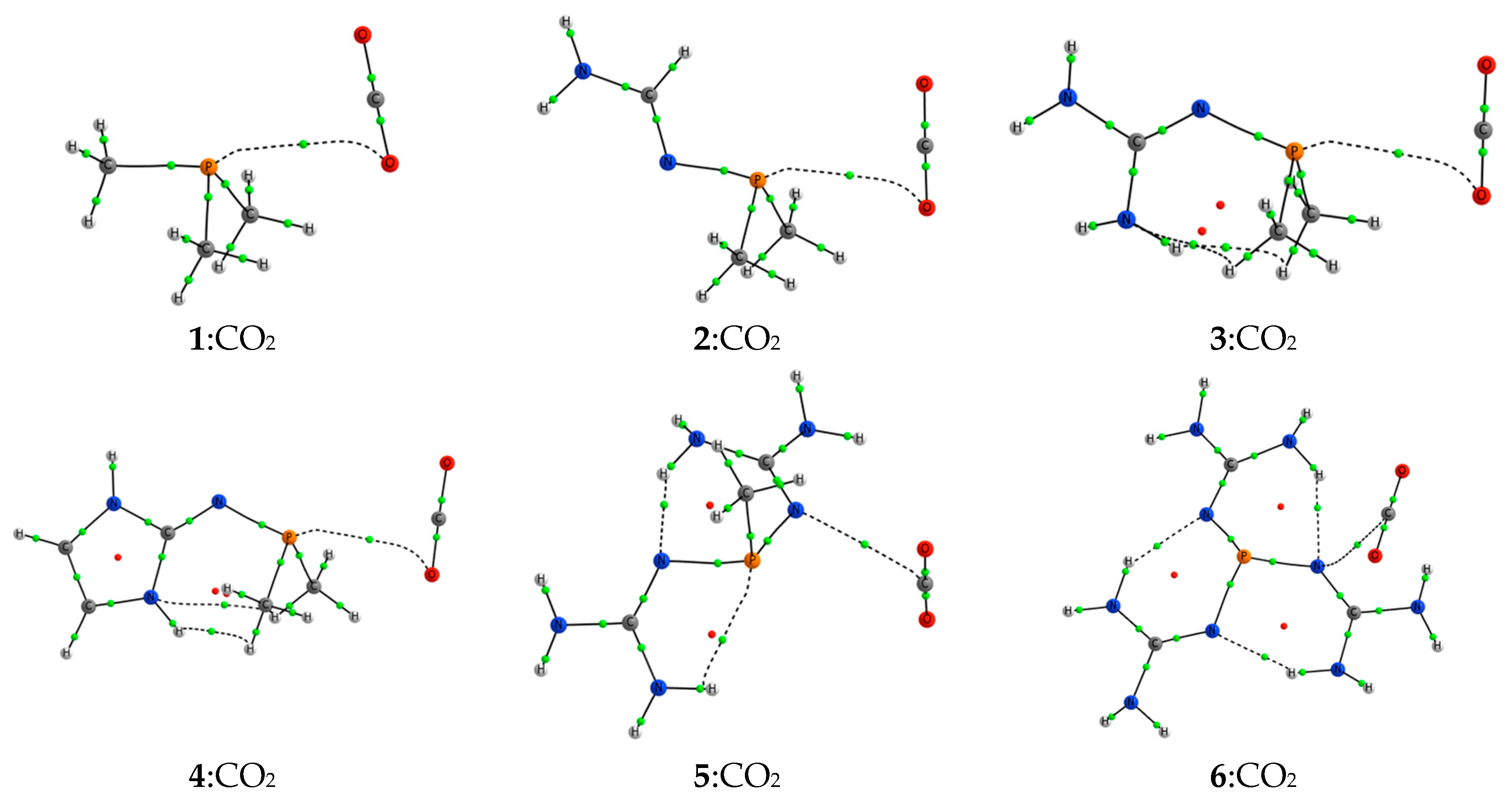
The complexes 2–4:CO2 show a pnicogen bond between the electrons of the oxygen atom of the CO2 and one of the σ-holes of the phosphorous atom of the phosphine, as in the case of 1:CO2. In contrast, complexes 5:CO2 and 6:CO2 present a tetrel bond [53,54,55] in which the lone pair of one of the nitrogen atoms directly connected to the phosphorous atom interacts with the π-hole of the carbon atom of CO2. These results are confirmed by the molecular graphs (Figure 5) in which a bond path connecting both atoms is shown. Transition states (/) and adducts (-) show in all cases an intermolecular BCP connecting the phosphorous atom of the phosphine and the carbon of the CO2.
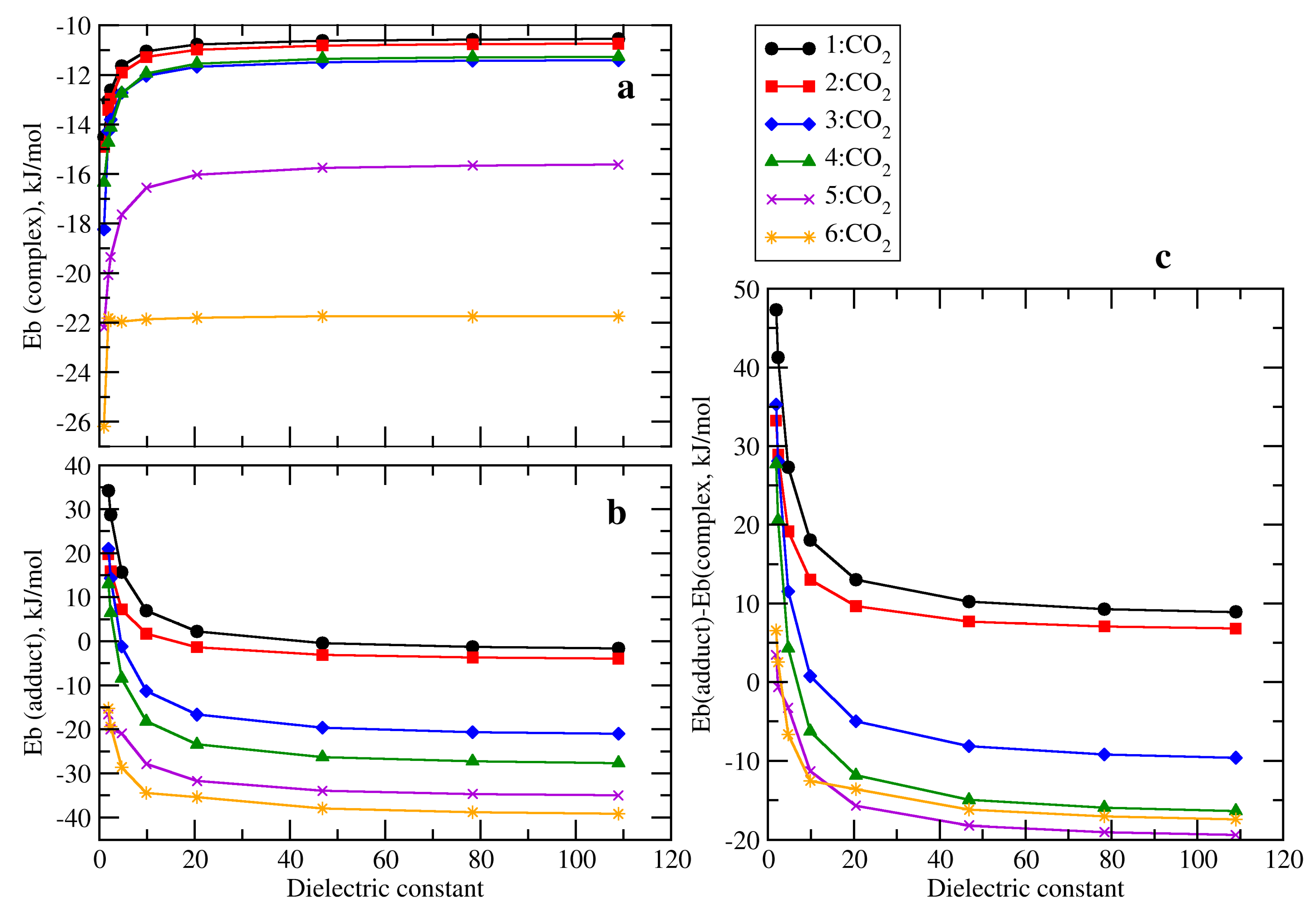
The evolution of the binding energies of the complexes and adducts considered vs. the solvent dielectric constant (Figure 6) is similar to the ones already described for the 1 + CO2 case; destabilization of the complex as the dielectric constant of the solvent increases (Figure 6a) and the other way around for the adduct (Figure 6b). Significant energetic variations from gas phase (ε = 1) to ε = 10 while the curves present a plateau for ε > 20 values have been observed. However, the different values obtained in gas phase that depend on the substituents of the phosphine are translated to the values in the plateau region. The binding energies obtained for all the complexes studied range between −26 (6:CO2) and −11 kJ·mol−1 (2:CO2), being the minimum and maximum values of each family as follows (Table S2): 2:CO2 (−14.9, −10.7), 3:CO2 (−18.2, −11.4), 4:CO2 (−16.4, −11.3), 5:CO2 (−22.2, −15.6), 6:CO2 (−26.2, −21.8). The energy range for n-CO2 adducts is larger than in the n:CO2 complexes between +35 and −39 kJ·mol−1, and also with respect to the complexes within the same family. Again, the extreme values correspond to 1 and 6. As mentioned above, solvation effects are different when complexes and adducts are considered. Complexes decrease on their binding energy with the increase of the dielectric constant in the solvent, while in adducts the tendency is the opposite: the larger the dielectric constant, the more negative binding energy. Also, as occurred for 1 + CO2, these results are associated to the small and large dipole moments found for the complexes and adducts, respectively.
The relative energy between the complex and the adduct with the dielectric constant of the solvent is shown in Figure 6c. As observed, for systems 1 and 2, curves are always positive, which indicated that the complex is always more stable than the adduct independently of the solvent considered. The 3:CO2 complex is more stable than the 3-CO2 adduct in solvents with ε < 10 but the adduct becomes more stable when ε < 10. Similar features were found for systems 4, 5, and 6 in which there is an inversion of the relative stability between complex and adduct from a certain value of the dielectric constant. Probably, the most interesting cases are 5 and 6 in which even at small values of ε the adduct is more stable than the complex.
A further inspection on the effect of the substituent on the binding energies has been carried out. When the substitution of methyl by amidine (from 1 to 2) is done, a decrease on the binding energies is observed in the complexes, TSs, and adducts across all the different solvents, being more pronounced in the latter than in the former. The substitution of a methyl by a guanidine (from 1 to 3) produces a larger decrease on the Eb in the complex independently of the solvent considered. In the adducts and TSs, this decrease is only observed for solvents with ε > 2.37, while in hexane and toluene, an increase on the Eb is shown for both type of structures. This is indicative of the dependency of more polar substituent with the solvents. Finally, when the c-Gua is considered, there is a drastic decrease on the Eb in all the systems.
Consider the series with an increasing number of guanidine substituents: 1, 3, 5, and 6 (Figure 7). In the absence of any solvent (Figure 7a, ε = 1) there is a linear decrease of the Eb in the complexes with the increase of the number of guanidine substituents (R2 = 0.9997). The Eb (complex) decreases (more negative) with the number of guanidines up to three (compound 6) where all the Eb becomes very similar. At any number of guanidines, the largest the dielectric constant of the solvent, the more positive is the Eb in the complex. Similarly, in case of adducts, the larger number of guanidines, the more negative Eb. However, in the limit case of three guanidines (compound 6) in the complex, the Eb was found very similar across the different solvents, while in the adduct, there is a clear separation between curves more pronounced at solvents with small dielectric constant values.
In the general case, the energetic variations of the two minima (complex and adduct) with the solvent are associated with a lengthening of the intermolecular distance in the complexes and with a shortening of the P–C bond in the adducts (see Table S3) as the dielectric constant of the solvent increases.
The transition barrier for the reaction accounted as the difference of energy between the complex and the TS structures (Figure 3) decreases with the polarity of the solvent due to the larger dipole moment found in the TS than in the complexes (Figures S2 and S3). Thus, the largest transition barrier is found for 1 + CO2 reaction in n-hexane model (52 kJ·mol−1) and the smallest one corresponds to 5 + CO2 reaction in formamide (25 kJ·mol−1). In fact, if we considered the evolution of the TS barriers with the number of guanidine groups across the different solvents (Figure S4), it is observed that the substitution of methyl groups by guanidines decreases considerably the transition barriers up to Me(Gua)2P:CO2 system. When the third methyl group is substituted there is an increase on the TS barriers, which may be due to sterical effects.
Regarding the interatomic P···C distance within the TS structures, the larger the interatomic distance, the larger the dielectric constant of the solvent, as was aforementioned for the 1 + CO2 case. If we analyse systems 2–6, there is a significant increase on the P···C distance (up to 0.2 Å) when moving from gas phase to n-hexane, and also increases with the dielectric constant of the solvent considered.
Excellent linear correlations are found between the P–C distance in the transition state geometries and the inverse of the dielectric constant of the solvent for the six cases considered (R2 > 0.99).
Since all the adducts and transition structures show a P–C BCP, it is possible to analyze the evolution of the electron density properties between 1.9 and 2.50 Å. Excellent exponential relationships are obtained between the P–C distance with ρBCP (R2 = 0.999) and with HBCP (R2 = 0.998), in agreement with previous reports [56,57,58].
Finally, to provide a more detailed view and feasibility of the reaction, Gibbs free energies (ΔG) have been obtained and summarized in Table S4. As observed, ΔG values are always positive when they are obtained with respect to the isolated monomers (entrance channel). This is well-known due to entropic effects of going from a more disordered system into a less disordered system (i.e., complexes, TSs, or adducts), but for all the stationary points, positive values of ΔG are obtained but for the most polar solvent, and for 6:CO2 adduct, the values are about 10 kJ/mol more stable than the ones obtained for the corresponding complexes as an indication that it should be possible to obtain such adducts. The ΔG values with respect to the complex, i.e., the configuration which leads eventually to the adduct connected by the transition barrier, show a different view. First, the reaction is more likely to be carried out under polar solvents as the TS barriers decrease with the dielectric constant of the solvent. Also, the adducts become more and more stable with the polarity of the solvent, showing an exothermic behaviour for compounds 5 in water and formamide and 6 in n-octanol, acetone, DMSO, water, and formamide. Again, the effect of the solvent is crucial in the stabilisation of the complexes, TSs, and adducts.
3. Methods
The geometry of the stationary points has been optimized at the Møller-Plesset MP2/aug’-cc-pVDZ computational level [59,60]. The aug’-cc-pVDZ basis set is built using the aug-cc-pVDZ basis set for heavy elements (C, N, O, and P in this article) and the cc-pVDZ for the hydrogens. In addition to the calculations in vacuum (ε = 1.0), the solvent effect on the reaction profile has been taken into account by means of the continuum polarizable method (PCM) [8] and the parameters of the hexane (ε = 1.88), toluene (ε = 2.37), chloroform (ε = 4.71), 1-octanol (ε = 9.86), acetone (ε = 20.49), dimethylsulfoxide (ε = 46.83), water (ε = 78.36), and formamide (ε = 108.94). In all cases, frequency calculations have been carried out to confirm that the geometry of the minima and TSs shows zero and only one imaginary frequency, respectively. Binding (electronic) energies and Gibbs free energies have been obtained as the difference between the energy of the complex (TS or adduct) minus the energy of the isolated monomers in the most stable configuration. All these calculations have been carried out with the Gaussian-16 program [61].
4. Conclusions
A thorough investigation of solvent effects on the reaction of different substituted RR’R’’P phosphines with CO2 has been carried out by means of MP2 calculations under PCM solvent models. For each energy profile, three different stationary points have been found. Of those, two correspond to minima structures, i.e., a pnicogen or tetrel bonded complex and a P–C bond adduct, and the third one was identified as a transition structure, which connects both minima structures.
The solvent effects on the stability and geometry of the stationary points are different. Thus, the complexes are destabilized as the dielectric constant of the solvent increases while the opposite happens with the adducts and the TSs.
Considering the substitution of one methyl group of (CH3)3P (1) by amidine (2), guanidine (3), or c-Gua (4), it was observed that replacing a CH3 by any of those leads to a decrease on the binding energies (more negative) in all the three modes (complexes, adducts, and TSs) across all the solvents. These effects are particularly pronounced when more than one CH3 is substituted (5 and 6).
Finally, ΔG values show that while the reaction is not favourable across some of the compounds (1–4), the solvent stabilises the adducts and TSs, mainly for polar solvents. Thus, compounds 5 and 6 showed negative values of ΔG indicating exothermic reactions.
Supplementary Materials
The following are available online at https://0-www-mdpi-com.brum.beds.ac.uk/2304-6740/6/4/110/s1, Figure S1: Linear (a) and second order polynomial (b) relationships between the Eb and 1/ε for the stationary points in the 1 + CO2 surface, Figure S2: Evolution of the transition barriers vs. the dielectric constant of the solvent, Figure S3: Evolution of the transition barriers vs. the complexes 1, 2, 3, and 4, Figure S4: Evolution of the transition barriers vs. the number of guanidine substituent for complexes 1, 3, 5, and 6, Table S1: Electron density properties (au) of the intermolecular BCP in the stationary points of the 1 + CO2 energy profile, Table S2: Binding energies (kJ·mol−1) and Linear relationship R2 vs. 1/ε of all the stationary points, Table S3: Interatomic distances (Å) in the stationary points, Table S4: Free Gibbs energies (ΔG) obtained with respect to the entrance channel (isolated monomers) and with respect to the complex configuration.
Author Contributions
Data curation, I.A., C.T., G.S.-S. and J.E.; Investigation, I.A., C.T., G.S.-S. and J.E.; Writing–original draft, I.A. and J.E.; Writing–review & editing, I.A., C.T., G.S.-S. and J.E.
Funding
This work was carried out with financial support from the Ministerio de Economía, Industria y Competitividad (Project No. CTQ2015-63997-C2-2-P) and Comunidad Autónoma de Madrid (S2013/MIT2841, Fotocarbon).
Acknowledgments
Thanks are also given to the CTI (CSIC) and to the Irish Centre for High-End Computing (ICHEC) for their continued computational support.
Conflicts of Interest
The authors declare no conflict of interest.
References
- Alkorta, I.; Elguero, J. 1,2-Proton shifts in pyrazole and related systems: A computational study of [1,5]-sigmatropic migrations of hydrogen and related phenomena. J. Chem. Soc. Perkin Trans. 2 1998, 2497–2504. [Google Scholar] [CrossRef]
- Trujillo, C.; Sánchez-Sanz, G.; Alkorta, I.; Elguero, J. Computational Study of Proton Transfer in Tautomers of 3- and 5-Hydroxypyrazole Assisted by Water. Chem. Phys. Chem. 2015, 16, 2140–2150. [Google Scholar] [CrossRef] [PubMed] [Green Version]
- Oziminski, W.P. The kinetics of water-assisted tautomeric 1,2-proton transfer in azoles: A computational approach. Struct. Chem. 2016, 27, 1845–1854. [Google Scholar] [CrossRef]
- Kamlet, M.J.; Abboud, J.L.; Taft, R.W. The solvatochromic comparison method. 6. The π* scale of solvent polarities. J. Am. Chem. Soc. 1977, 99, 6027–6038. [Google Scholar] [CrossRef]
- Reichardt, C. Solvatochromic Dyes as Solvent Polarity Indicators. Chem. Rev. 1994, 94, 2319–2358. [Google Scholar] [CrossRef]
- Abraham, M.H. Hydrogen bonding. 31. Construction of a scale of solute effective or summation hydrogen-bond basicity. J. Phys. Org. Chem. 1993, 6, 660–684. [Google Scholar] [CrossRef]
- Catalán, J. Toward a Generalized Treatment of the Solvent Effect Based on Four Empirical Scales: Dipolarity (SdP, a New Scale), Polarizability (SP), Acidity (SA), and Basicity (SB) of the Medium. J. Phys. Chem. 2009, 113, 5951–5960. [Google Scholar] [CrossRef] [PubMed]
- Tomasi, J.; Mennucci, B.; Cammi, R. Quantum Mechanical Continuum Solvation Models. Chem. Rev. 2005, 105, 2999–3094. [Google Scholar] [CrossRef] [PubMed]
- Orozco, M.; Luque, F.J. Theoretical Methods for the Description of the Solvent Effect in Biomolecular Systems. Chem. Rev. 2000, 100, 4187–4226. [Google Scholar] [CrossRef] [PubMed]
- Zhu, T.; Li, J.; Hawkins, G.D.; Cramer, C.J.; Truhlar, D.G. Density functional solvation model based on CM2 atomic charges. J. Phys. Chem. 1998, 109, 9117–9133. [Google Scholar] [CrossRef]
- Sánchez-Sanz, G.; Trujillo, C. Improvement of Anion Transport Systems by Modulation of Chalcogen Interactions: The influence of solvent. J. Phys. Chem. 2018, 122, 1369–1377. [Google Scholar] [CrossRef] [PubMed]
- Sun, Z.-H.; Albrecht, M.; Raabe, G.; Pan, F.-F.; Räuber, C. Solvent-Dependent Enthalpic versus Entropic Anion Binding by Biaryl Substituted Quinoline Based Anion Receptors. J. Phys. Chem. 2015, 119, 301–306. [Google Scholar] [CrossRef] [PubMed]
- Liu, Y.-Z.; Yuan, K.; Lv, L.-L.; Zhu, Y.-C.; Yuan, Z. Designation and Exploration of Halide–Anion Recognition Based on Cooperative Noncovalent Interactions Including Hydrogen Bonds and Anion−π. J. Phys. Chem. 2015, 119, 5842–5852. [Google Scholar] [CrossRef] [PubMed]
- Lu, Y.; Li, H.; Zhu, X.; Liu, H.; Zhu, W. Effects of solvent on weak halogen bonds: Density functional theory calculations. Int. J. Quantum Chem. 2011, 112, 1421–1430. [Google Scholar] [CrossRef]
- Sánchez-Sanz, G.; Crowe, D.; Nicholson, A.; Fleming, A.; Carey, E.; Kelleher, F. Conformational studies of Gram-negative bacterial quorum sensing acyl homoserine lactone (AHL) molecules: The importance of the n→ π* interaction. Biophys. Chem. 2018, 238, 16–21. [Google Scholar] [CrossRef] [PubMed]
- Crowe, D.; Nicholson, A.; Fleming, A.; Carey, E.; Sánchez-Sanz, G.; Kelleher, F. Conformational studies of Gram-negative bacterial quorum sensing 3-oxo N-acyl homoserine lactone molecules. Biorg. Med. Chem. 2017, 25, 4285–4296. [Google Scholar] [CrossRef] [PubMed]
- Keeling, C.D.; Bacastrow, R.B. Energy and Climate: Studies in Geophysics. In Impact of Industrial Gases on Climate; The National Academies Press: Washington, DC, USA, 1977; pp. 72–95. [Google Scholar]
- Keeling, R.F.; Shertz, S.R. Seasonal and interannual variations in atmospheric oxygen and implications for the global carbon cycle. Nature 1992, 358, 723. [Google Scholar] [CrossRef]
- Keeling, C.D.; Whorf, T.P.; Wahlen, M.; van der Plichtt, J. Interannual extremes in the rate of rise of atmospheric carbon dioxide since 1980. Nature 1995, 375, 666. [Google Scholar] [CrossRef]
- Keeling, R.F.; Piper, S.C.; Heimann, M. Global and hemispheric CO2 sinks deduced from changes in atmospheric O2 concentration. Nature 1996, 381, 218. [Google Scholar] [CrossRef]
- Keeling, C.D.; Chin, J.F.S.; Whorf, T.P. Increased activity of northern vegetation inferred from atmospheric CO2 measurements. Nature 1996, 382, 146. [Google Scholar] [CrossRef]
- Keeling, R.F. Recording Earth’s Vital Signs. Science 2008, 319, 1771–1772. [Google Scholar] [CrossRef] [PubMed]
- Anderson, T.R.; Hawkins, E.; Jones, P.D. CO2, the greenhouse effect and global warming: From the pioneering work of Arrhenius and Callendar to today's Earth System Models. Endeavour 2016, 40, 178–187. [Google Scholar] [CrossRef] [PubMed] [Green Version]
- Heard, D.E.; Saiz-Lopez, A. Atmospheric chemistry. Chem. Soc. Rev. 2012, 41, 6229–6230. [Google Scholar] [CrossRef] [PubMed]
- Artz, J.; Müller, T.E.; Thenert, K.; Kleinekorte, J.; Meys, R.; Sternberg, A.; Bardow, A.; Leitner, W. Sustainable Conversion of Carbon Dioxide: An Integrated Review of Catalysis and Life Cycle Assessment. Chem. Rev. 2018, 118, 434–504. [Google Scholar] [CrossRef] [PubMed]
- Tomasko, D.L.; Li, H.; Liu, D.; Han, X.; Wingert, M.J.; Lee, L.J.; Koelling, K.W. A Review of CO2 Applications in the Processing of Polymers. Ind. Eng. Chem. Res. 2003, 42, 6431–6456. [Google Scholar] [CrossRef]
- Yang, H.; Xu, Z.; Fan, M.; Gupta, R.; Slimane, R.B.; Bland, A.E.; Wright, I. Progress in carbon dioxide separation and capture: A review. J. Environ. Sci. 2008, 20, 14–27. [Google Scholar] [CrossRef]
- Kanki, K.; Maki, H.; Mizuhata, M. Carbon dioxide absorption behavior of surface-modified lithium orthosilicate/potassium carbonate prepared by ball milling. Int. J. Hydrog. Energy 2016, 41, 18893–18899. [Google Scholar] [CrossRef]
- Tang, Z.; Lu, L.; Dai, Z.; Xie, W.; Shi, L.; Lu, X. CO2 Absorption in the Ionic Liquids Immobilized on Solid Surface by Molecular Dynamics Simulation. Langmuir 2017, 33, 11658–11669. [Google Scholar] [CrossRef] [PubMed]
- Lawlor, D.W.; Mitchell, R.A.C. The effects of increasing CO2 on crop photosynthesis and productivity: A review of field studies. Plant Cell Environ. 1991, 14, 807–818. [Google Scholar] [CrossRef]
- Shukla, R.; Ranjith, P.; Haque, A.; Choi, X. A review of studies on CO2 sequestration and caprock integrity. Fuel 2010, 89, 2651–2664. [Google Scholar] [CrossRef]
- Chen, K.-H.; Tam, K.-W.; Chen, I.f.; Huang, S.K.; Tzeng, P.-C.; Wang, H.-J.; Chen, C. A systematic review of comparative studies of CO2 and erbium:YAG lasers in resurfacing facial rhytides (wrinkles). J. Cosmet. Laser Ther. 2017, 19, 199–204. [Google Scholar] [CrossRef] [PubMed]
- Wang, M.; Lawal, A.; Stephenson, P.; Sidders, J.; Ramshaw, C. Post-combustion CO2 capture with chemical absorption: A state-of-the-art review. Chem. Eng. Res. Des. 2011, 89, 1609–1624. [Google Scholar] [CrossRef] [Green Version]
- Ingrosso, F.; Ruiz-López, M.F. Electronic Interactions in Iminophosphorane Superbase Complexes with Carbon Dioxide. J. Phys. Chem. A 2018, 122, 1764–1770. [Google Scholar] [CrossRef] [PubMed]
- Azofra, L.M.; Scheiner, S. Complexes containing CO2 and SO2. Mixed dimers, trimers and tetramers. Phys. Chem. Chem. Phys. 2014, 16, 5142–5149. [Google Scholar] [CrossRef] [PubMed]
- Alkorta, I.; Blanco, F.; Elguero, J.; Dobado, J.A.; Ferrer, S.M.; Vidal, I. Carbon···Carbon Weak Interactions. J. Phys. Chem. A 2009, 113, 8387–8393. [Google Scholar] [CrossRef] [PubMed] [Green Version]
- Del Bene, J.E.; Alkorta, I.; Elguero, J. Carbenes as Electron-Pair Donors To CO2 for C···C Tetrel Bonds and C–C Covalent Bonds. J. Phys. Chem. A 2017, 121, 4039–4047. [Google Scholar] [CrossRef] [PubMed]
- Alkorta, I.; Elguero, J.; Del Bene, J.E. Azines as Electron-Pair Donors to CO2 for N···C Tetrel Bonds. J. Phys. Chem. A 2017, 121, 8017–8025. [Google Scholar] [CrossRef] [PubMed]
- Del Bene, J.E.; Alkorta, I.; Elguero, J. Carbon–Carbon Bonding between Nitrogen Heterocyclic Carbenes and CO2. J. Phys. Chem. A 2017, 121, 8136–8146. [Google Scholar] [CrossRef] [PubMed]
- Alkorta, I.; Montero-Campillo, M.M.; Elguero, J. Trapping CO2 by Adduct Formation with Nitrogen Heterocyclic Carbenes (NHCs): A Theoretical Study. Chem. Eur. J. 2017, 23, 10604–10609. [Google Scholar] [CrossRef] [PubMed]
- Montero-Campillo, M.M.; Alkorta, I.; Elguero, J. Binding indirect greenhouse gases OCS and CS2 by nitrogen heterocyclic carbenes (NHCs). PCCP 2018, 20, 19552–19559. [Google Scholar] [CrossRef] [PubMed]
- Pu, M.; Privalov, T. Ab Initio Molecular Dynamics with Explicit Solvent Reveals a Two-Step Pathway in the Frustrated Lewis Pair Reaction. Chem. Eur. J. 2015, 21, 17708–17720. [Google Scholar] [CrossRef] [PubMed]
- Denning, D.M.; Falvey, D.E. Solvent-Dependent Decarboxylation of 1,3-Dimethylimdazolium-2-Carboxylate. J. Org. Chem. 2014, 79, 4293–4299. [Google Scholar] [CrossRef] [PubMed]
- Denning, D.M.; Falvey, D.E. Substituent and Solvent Effects on the Stability of N-Heterocyclic Carbene Complexes with CO2. J. Org. Chem. 2017, 82, 1552–1557. [Google Scholar] [CrossRef] [PubMed]
- Torrent-Sucarrat, M.; Varandas, A.J.C. Carbon Dioxide Capture and Release by Anions with Solvent-Dependent Behaviour: A Theoretical Study. Chem. Eur. J. 2016, 22, 14056–14063. [Google Scholar] [CrossRef] [PubMed]
- Buß, F.; Mehlmann, P.; Mück-Lichtenfeld, C.; Bergander, K.; Dielmann, F. Reversible Carbon Dioxide Binding by Simple Lewis Base Adducts with Electron-Rich Phosphines. J. Am. Chem. Soc. 2016, 138, 1840–1843. [Google Scholar] [CrossRef] [PubMed]
- Mehlmann, P.; Mück-Lichtenfeld, C.; Tan, T.T.Y.; Dielmann, F. Tris(imidazolin-2-ylidenamino)phosphine: A Crystalline Phosphorus(III) Superbase That Splits Carbon Dioxide. Chem. Eur. J. 2017, 23, 5929–5933. [Google Scholar] [CrossRef] [PubMed]
- Tolman, C.A. Steric effects of phosphorus ligands in organometallic chemistry and homogeneous catalysis. Chem. Rev. 1977, 77, 313–348. [Google Scholar] [CrossRef]
- Scheiner, S. A new noncovalent force: Comparison of P···N interaction with hydrogen and halogen bonds. J. Chem. Phys. 2011, 134, 094315. [Google Scholar] [CrossRef] [PubMed]
- Zahn, S.; Frank, R.; Hey-Hawkins, E.; Kirchner, B. Pnicogen Bonds: A New Molecular Linker? Chem. Eur. J. 2011, 17, 6034–6038. [Google Scholar] [CrossRef] [PubMed]
- Del Bene, J.E.; Alkorta, I.; Elguero, J. The Pnicogen Bond in Review: Structures, Binding Energies, Bonding Properties, and Spin-Spin Coupling Constants of Complexes Stabilized by Pnicogen Bonds. In Noncovalent Forces; Scheiner, S., Ed.; Springer International Publishing: Cham, Switzerland, 2015; pp. 191–263. [Google Scholar]
- Sánchez-Sanz, G.; Trujillo, C.; Alkorta, I.; Elguero, J. Electron density shift description of non-bonding intramolecular interactions. Comput. Theor. Chem. 2012, 991, 124–133. [Google Scholar] [CrossRef] [Green Version]
- Legon, A.C. Tetrel, pnictogen and chalcogen bonds identified in the gas phase before they had names: A systematic look at non-covalent interactions. PCCP 2017, 19, 14884–14896. [Google Scholar] [CrossRef] [PubMed]
- Alkorta, I.; Rozas, I.; Elguero, J. Molecular Complexes between Silicon Derivatives and Electron-Rich Groups. J. Phys. Chem. A 2001, 105, 743–749. [Google Scholar] [CrossRef]
- Bauzá, A.; Mooibroek, T.J.; Frontera, A. Tetrel-Bonding Interaction: Rediscovered Supramolecular Force? Angew. Chem. Int. Ed. 2013, 52, 12317–12321. [Google Scholar] [CrossRef] [PubMed]
- Alkorta, I.; Barrios, L.; Rozas, I.; Elguero, J. Comparison of models to correlate electron density at the bond critical point and bond distance. J. Mol. Struc. THEOCHEM 2000, 496, 131–137. [Google Scholar] [CrossRef]
- Espinosa, E.; Alkorta, I.; Elguero, J.; Molins, E. From weak to strong interactions: A comprehensive analysis of the topological and energetic properties of the electron density distribution involving X–H⋯F–Y systems. J. Chem. Phys. 2002, 117, 5529–5542. [Google Scholar] [CrossRef]
- Alkorta, I.; Solimannejad, M.; Provasi, P.; Elguero, J. Theoretical study of complexes and fluoride cation transfer between N2F+ and electron donors. J. Phys. Chem. A 2007, 111, 7154–7161. [Google Scholar] [CrossRef] [PubMed]
- Møller, C.; Plesset, M.S. Note on an Approximation Treatment for Many-Electron Systems. Phys. Rev. 1934, 46, 618–622. [Google Scholar] [CrossRef] [Green Version]
- Dunning, T.H. Gaussian-Basis Sets for Use in Correlated Molecular Calculations. 1. The Atoms Boron through Neon and Hydrogen. J. Chem. Phys. 1989, 90, 1007–1023. [Google Scholar] [CrossRef]
- Frisch, M.J.; Trucks, G.W.; Schlegel, H.B.; Scuseria, G.E.; Robb, M.A.; Cheeseman, J.R.; Scalmani, G.; Barone, V.; Petersson, G.A.; Nakatsuji, H.; et al. Gaussian 16; Gaussian Inc.: Wallingford, CT, USA, 2016. [Google Scholar]
- Keith, T.A. AIMAll; 17.11.14B; TK Gristmill Software: Overland Park, KS, USA; Available online: http://aim.tkgristmill.com/ (accessed on 12 April 2018).
- Jmol: An Open-Source Java Viewer for Chemical Structures in 3D. Available online: http://www.jmol.org/ (accessed on 12 April 2018).
Figure 1.
Imidazolin-2-ylidenamino substituted phosphines (IAPs).

Figure 2.
Schematic representation of the phosphines studied.

Figure 3.
Optimized stationary points along 1 + CO2 energy profile using continuum polarizable method (PCM)-chloroform solvent model.
Figure 3.
Optimized stationary points along 1 + CO2 energy profile using continuum polarizable method (PCM)-chloroform solvent model.

Figure 4.
Electron density shift maps for the stationary points of the 1 + CO2 energy profile. Positive and negative values are shown in blue and yellow, respectively. The surfaces for the complex correspond to ±0.0002 au and in the transition state (TS) and adduct to ±0.002 au.
Figure 4.
Electron density shift maps for the stationary points of the 1 + CO2 energy profile. Positive and negative values are shown in blue and yellow, respectively. The surfaces for the complex correspond to ±0.0002 au and in the transition state (TS) and adduct to ±0.002 au.

Figure 5.
Molecular graphs for the 1–6:CO2 complexes. The small green and red spheres represent the position of the bond and ring critical points, respectively.
Figure 5.
Molecular graphs for the 1–6:CO2 complexes. The small green and red spheres represent the position of the bond and ring critical points, respectively.

Figure 6.
(a) Evolution of the binding energies of the complex; (b) Adduct vs. the dielectric constant of the solvent; (c) Relative energy between the complex and adduct for each system vs. the dielectric constant of the solvent. In-plot: zoom into the inner region with low dielectric constant.
Figure 6.
(a) Evolution of the binding energies of the complex; (b) Adduct vs. the dielectric constant of the solvent; (c) Relative energy between the complex and adduct for each system vs. the dielectric constant of the solvent. In-plot: zoom into the inner region with low dielectric constant.

Figure 7.
Evolution of the binding energies of the complex (a) and adduct (b) vs. number or guanidine substituents for systems 1, 3, 5, and 6.
Figure 7.
Evolution of the binding energies of the complex (a) and adduct (b) vs. number or guanidine substituents for systems 1, 3, 5, and 6.


Table 1.
Binding energy, Eb, (kJ·mol−1) and P···C and P···O intermolecular distances (Å) of 1 + CO2 stationary points in different solvent models.
Table 1.
Binding energy, Eb, (kJ·mol−1) and P···C and P···O intermolecular distances (Å) of 1 + CO2 stationary points in different solvent models.
| Solvent | 1:CO2 | 1/CO2 | 1-CO2 | ||||
|---|---|---|---|---|---|---|---|
| Eb | P···C | P···O | Eb | P···C | Eb | P···C | |
| Gas | −14.5 | 3.365 | 3.306 | ||||
| Hexane | −13.1 | 3.367 | 3.323 | 38.5 | 2.206 | 34.2 | 1.959 |
| Toluene | −12.6 | 3.372 | 3.332 | 36.0 | 2.245 | 28.7 | 1.946 |
| Chloroform | −11.6 | 3.387 | 3.349 | 31.6 | 2.318 | 15.7 | 1.926 |
| 1-Octanol | −11.1 | 3.397 | 3.362 | 29.5 | 2.358 | 7.0 | 1.917 |
| Acetone | −10.8 | 3.405 | 3.370 | 28.7 | 2.377 | 2.2 | 1.914 |
| Dimethylsulfoxide, DMSO | −10.6 | 3.409 | 3.374 | 28.2 | 2.387 | −0.4 | 1.912 |
| Water | −10.6 | 3.410 | 3.375 | 28.1 | 2.390 | −1.3 | 1.911 |
| Formamide | −10.6 | 3.410 | 3.374 | 28.1 | 2.391 | −1.6 | 1.911 |
© 2018 by the authors. Licensee MDPI, Basel, Switzerland. This article is an open access article distributed under the terms and conditions of the Creative Commons Attribution (CC BY) license (http://creativecommons.org/licenses/by/4.0/).
Share and Cite
MDPI and ACS Style
Alkorta, I.; Trujillo, C.; Sánchez-Sanz, G.; Elguero, J. Solvent and Substituent Effects on the Phosphine + CO2 Reaction. Inorganics 2018, 6, 110. https://0-doi-org.brum.beds.ac.uk/10.3390/inorganics6040110
AMA Style
Alkorta I, Trujillo C, Sánchez-Sanz G, Elguero J. Solvent and Substituent Effects on the Phosphine + CO2 Reaction. Inorganics. 2018; 6(4):110. https://0-doi-org.brum.beds.ac.uk/10.3390/inorganics6040110
Chicago/Turabian StyleAlkorta, Ibon, Cristina Trujillo, Goar Sánchez-Sanz, and José Elguero. 2018. "Solvent and Substituent Effects on the Phosphine + CO2 Reaction" Inorganics 6, no. 4: 110. https://0-doi-org.brum.beds.ac.uk/10.3390/inorganics6040110
Note that from the first issue of 2016, this journal uses article numbers instead of page numbers. See further details here.