A Continuum from Halogen Bonds to Covalent Bonds: Where Do λ3 Iodanes Fit?


1
Department of Chemistry, Southern Methodist University, 3215 Daniel Avenue, Dallas, TX 75275-0314, USA
2
Instituto Tecnológico de Aeronáutica (ITA), Departamento de Química, São José dos Campos, 12228-900 São Paulo, Brazil
*
Author to whom correspondence should be addressed.
Inorganics 2019, 7(4), 47; https://0-doi-org.brum.beds.ac.uk/10.3390/inorganics7040047
Submission received: 14 February 2019
/
Revised: 8 March 2019
/
Accepted: 15 March 2019
/
Published: 28 March 2019
(This article belongs to the Special Issue Halogen Bonding: Fundamentals and Applications)
Abstract
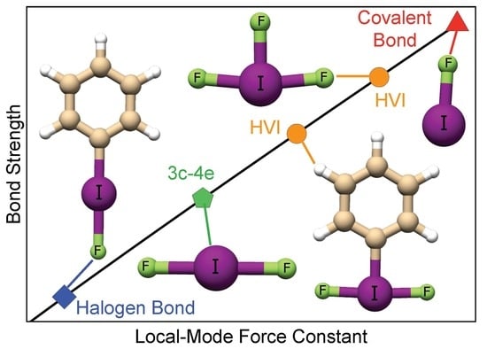
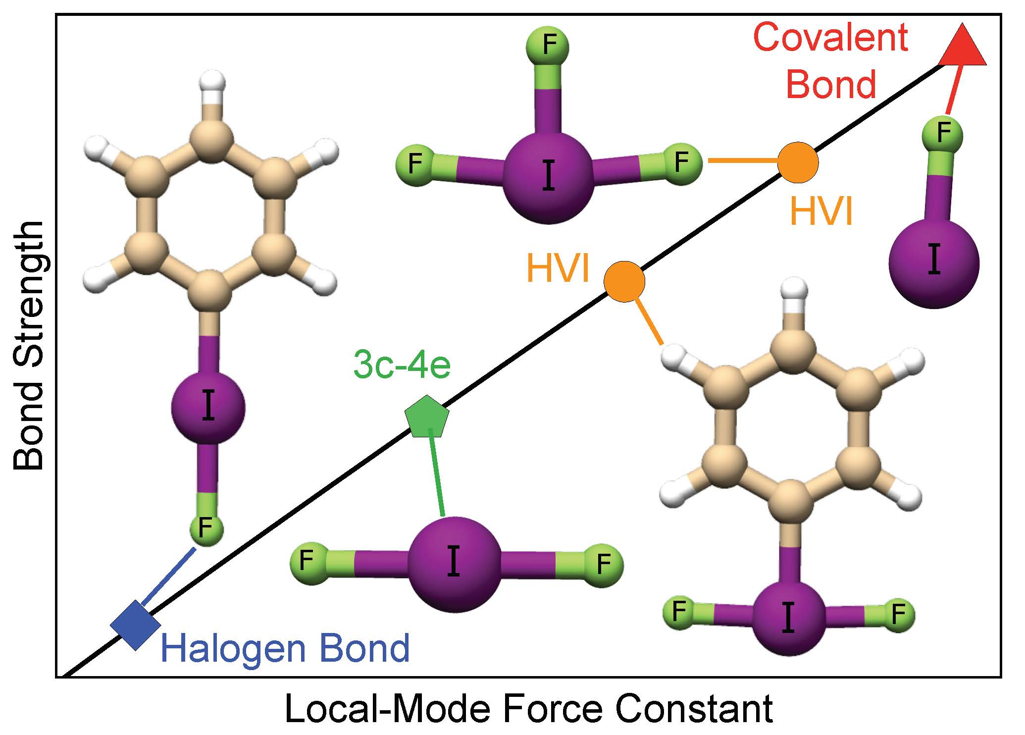
:The intrinsic bonding nature of -iodanes was investigated to determine where its hypervalent bonds fit along the spectrum between halogen bonding and covalent bonding. Density functional theory with an augmented Dunning valence triple zeta basis set (B97X-D/aug-cc-pVTZ) coupled with vibrational spectroscopy was utilized to study a diverse set of 34 hypervalent iodine compounds. This level of theory was rationalized by comparing computational and experimental data for a small set of closely-related and well-studied iodine molecules and by a comparison with CCSD(T)/aug-cc-pVTZ results for a subset of the investigated iodine compounds. Axial bonds in -iodanes fit between the three-center four-electron bond, as observed for the trihalide species IF and the covalent FI molecule. The equatorial bonds in -iodanes are of a covalent nature. We explored how the equatorial ligand and axial substituents affect the chemical properties of -iodanes by analyzing natural bond orbital charges, local vibrational modes, the covalent/electrostatic character, and the three-center four-electron bonding character. In summary, our results show for the first time that there is a smooth transition between halogen bonding → 3c–4e bonding in trihalides → 3c–4e bonding in hypervalent iodine compounds → covalent bonding, opening a manifold of new avenues for the design of hypervalent iodine compounds with specific properties.
1. Introduction
Hypervalent iodine compounds (HVI) are important alternatives to transition metal reagents because of their reactivity, synthetic utility, low cost, abundance, and non-toxic nature [1,2,3,4,5,6]. HVIs are involved in a multitude of reactions such as: reductive elimination, ligand exchange, oxidative addition, and ligand coupling [7,8]. The three-center four-electron bonds (3c–4e) in HVI are weak and polarizable, which is valuable in synthetic organic chemistry, as they can exchange leaving groups or accept electrophilic/nucleophilic ligands depending on their surroundings [9]. Despite such utility, there are still unknowns regarding the intrinsic bonding nature of HVIs and hypervalency in general. Though iodine is a halogen, it behaves like a metal; it is the heaviest non-radioactive element of the periodic table and is the most polarizable halogen [10,11]. Because of its diffuse electron density (van der Waals (vdW) radius of ca 2 Å), iodine is a good electron donor, but can also serve as an electron acceptor [12,13]. Iodine is not known to participate in d-orbital or -interactions, though this could be further investigated [14,15].
HVIs commonly exist in the oxidation states 3, 5, and 7, which support 10, 12, and 14 valence electrons, respectively [16]. Most common are the oxidation states 3 and 5, which are referred to as and -iodanes [17]. -iodanes form distorted T-shaped molecular geometries, while -iodanes generally prefer square pyramidal geometries, as confirmed through both X-ray crystallography and computational studies [18,19]. These somewhat unusual molecular geometries are the result of the pseudo-Jahn–Teller effect [20]. The atoms that make up the “T” in -iodanes form improper dihedrals and non-ideal bond angles. The causes of these angular and dihedral deviations are unknown, but have been related to the anisotropic nature of the electronic density distribution in iodine [21,22,23,24,25]. Bader et al. showed that the vdW radius in iodine is larger at the equatorial position than at the axial position [26,27,28]. This supports the observation that electronegative ligands favor the axial positions in iodine [29].
Hypervalency has been defined in several ways: Musher characterized main group elements in higher oxidation states as hypervalent [30]. A successful concept employed to explain hypervalency without involving d-orbitals is the formation of multi-centered electron-deficient bonds [31,32,33]. In this context, the 3c–4e bond model of Pimentel–Rundle is especially useful. According to this model, three atoms linearly align, each of which contributes an atomic orbital to form three molecular orbitals; a bonding orbital, a non-bonding orbital, and an antibonding orbital. Since only four electrons are involved, the antibonding orbital is unoccupied. As a result, two bonds share a single bonding electron pair (i.e., they have a fractional bond order of 0.5). The formation of two or more electron-deficient bonds allows hypervalent compounds to have higher oxidation states without necessarily expanding their octets. A direct consequence of this model is that the 3c–4e bond is expected to be substantially weaker than the two-center two-electron (2c–2e) bond in a given hypervalent molecule. Even though there are various works showing that d-orbital contributions to hypervalent bonds (HVB) are minimal, many chemistry text books still make use of the idea of an extended octet and the formation of spd-hybrid orbitals to explain HVB [34]. There is a strong overlap between the concepts of fractional bond order, the 3c–4e bond, and the halogen bond (XB) in trihalides, which are considered prime examples of 3c–4e bonding, but also strong XB [35,36]. A formal definition of XB is given in the following paragraph.
3c–4e HVI bonding (3c–4e HVIB) draws comparisons to the secondary bonding interaction due to the weak bond strength, high reactivity, and long internuclear distances exceeding covalent bond lengths [37]. 3c–4e HVIB also shares similarities with non-covalent interactions, along with hydrogen bonding [38,39,40], XB [35,41,42,43], pnicogen bonding [43,44,45], chalcogen bonding [43,46], and tetrel bonding [47]. XB is a non-covalent interaction between an electrophilic halogen (X) and a nucleophile with a lone pair (lp(A)) of donating electrons [42,43]. For the remainder of this work, we will express lone pairs as (lp).The nucleophile/halogen acceptor (A), donates electrons to the antibonding (*(XY)) orbital of the halogen donor (Y) [48,49]. XB is also known to have an X–A distance that is shorter than the sum of the vdW radii with Y–X–A angles close to 180 degrees [35,41,50,51]. Because of the obvious similarities between 3c–4e HVIB and XB, it has been argued that HVB should not be considered as a special bonding class [52,53]. On the other hand, the term hypervalency has been widely accepted by the chemistry community, and therefore, its continuous use has been advocated [54]. Based on this controversy, we decided to delve deeper into the bonding nature of -iodanes.
In this work, we investigated the intrinsic nature of HVIB in -iodanes and its relation to XB, 3c–4e bonding in trihalides, and covalent bonding to determine if there is a smooth transition between these interactions. Additionally, we studied the role equatorial ligands play in strengthening the 3c–4e bond in -iodanes, as well as substituent effects in the axial ligands. We utilized density functional theory (DFT), vibrational spectroscopy, quantum theory of atoms in molecules (QTAIM) combined with the Cremer–Kraka criterion for covalent bonding [55,56,57], and the natural bond orbital (NBO) analysis to characterize the nature and the intrinsic strength of HVIB. This investigation was rationalized by studying a diverse group of 34 HVI compounds shown in Figure 1, including known chemical compounds complemented by some model compounds. The remainder of this work is presented as follows: data, results, and discussion are presented in Section 2; Section 3 gives a description of the computational methods utilized; and Section 4 gives conclusions, the outlook, and future goals.
2. Results and Discussion
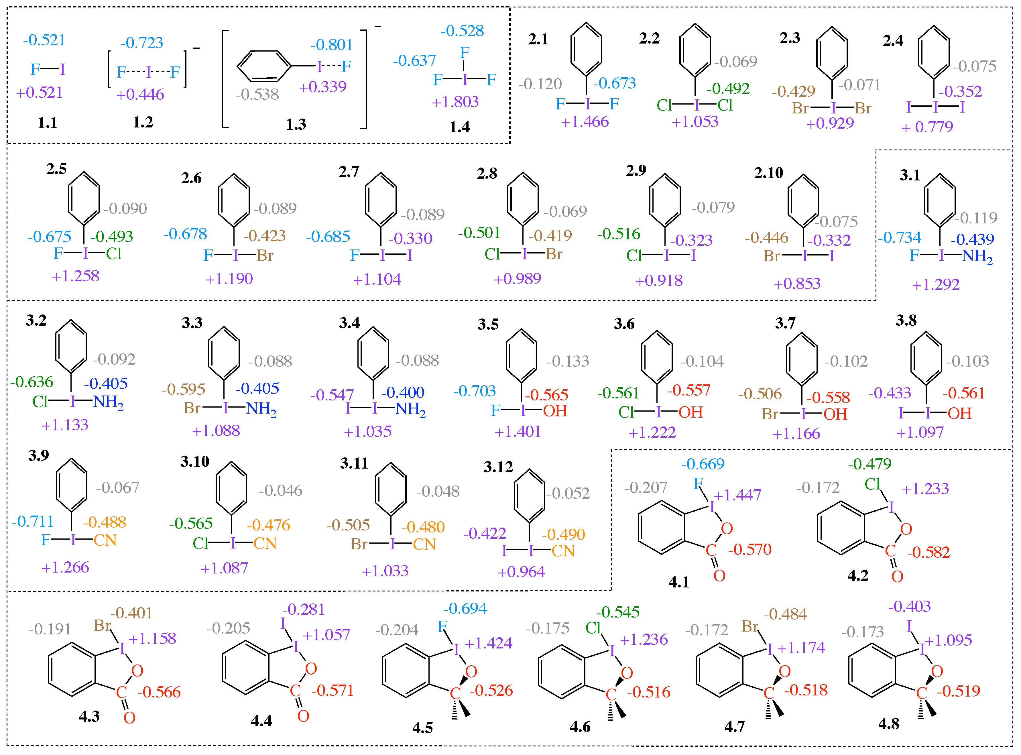
Figure 1 shows the 34 HVI compounds with selected NBO charges investigated in this work. Note that the abbreviation (PhI) is used to refer to iodobenzenes.
The compounds are organized into four groups. Group 1 contains four reference compounds; the covalent complex FI (1.1), the 3c–4e trihalide IF (1.2), fluorophenyl iodide (1.3), and the -iodane, IF (1.4), which is used to study the effects of electronegative equatorial ligands. Group 2 and Group 3 compounds, iodobenzenes (2.1–2.10) and (3.1–3.11), respectively, represent -iodanes with a phenyl group equatorially bound to I. While both axial ligands in Group 2 molecules are halogen atoms, in Group 3, the axial ligands consist of a halogen and a non-halogen lone-pair-bearing functional group (CN, NH, and OH). Group 4 consists of four halobenziodazoles (4.1–4.4) and four halobenziodoxoles (4.5–4.8).
2.1. NBO Charge Analysis
XB is a non-covalent interaction formed between a halogen donor molecule (YX) (e.g., a dihalogen, interhalogen, or halogenated molecule) and a halogen acceptor atom A, where A is an electron-rich atom; e.g., a nucleophilic heteroatom with lone-pair (lp) electrons [9,35,41,42,43]. The general charge transfer picture in XB describes a transfer of charge from lp (A) into the empty (YX) orbital [36,58,59]. Applied to our set of HVI compounds, there are two possibilities to define the YI and the IA part of Group 2 molecules 2.5–2.10. In these cases, we chose IA to be the weaker of the two axial bonds, in analogy to XB. The same definition was also applied for Group 3 and Group 4 compounds.
For all 34 HVI compounds investigated in this work, the central iodine atom I holds a positive charge (see purple numbers in Figure 1), ranging from +0.339 e in 1.3 to +1.803 e in 1.4. There is a significant difference in the central iodine charge when comparing the -iodanes with the three reference compounds 1.1–1.3 for which the iodine charge ranges from +0.339 e to +0.521 e, whereas iodine charges in -iodanes range from +0.779 e in 2.4 to +1.803 e in 1.4. The obvious difference between the HVIs and the non-HVIs is the equatorial ligand, which is absent in 1.1–1.3. In every case, except 1.4, the equatorial ligand is a phenyl (Ph) group (Groups 2–3) or a benzene ring (Group 4). Group charges for Ph/benzene ligands are negative in every case, as are charges on the Ph/benzene C atom bound to I, as shown in Figure 1. Increased positive charge on I indicates that the equatorial ligands are pulling charge from the central I. In 1.4, the equatorial ligand is F; this is an extreme case of a strong electron-withdrawing ligand in the equatorial position, which polarizes the central I atom. As a result, each I–F interaction involved in the 3c–4e bond becomes more polar.
2.1–2.4 comprise -iodanes of the type PhIA, for A = F, Cl, Br, and I. Caused by the increasing electronegativity from I to F, the bond polarity increases from I–I < Br–I < Cl–I < F–I, with the positive charge on the central I atom increasing in the same order, i.e., +0.779 e in 2.4 to +1.466 e in 2.1. The same trend is observed in 2.5–2.7. As the second substituent changes from Cl to I, charge on the F ligand remains almost unchanged (q = −0.012 e), while the positive charge on I decreases. The same pattern continues for compounds 2.8–2.10. The charge on the equatorial ligand appears to be independent of the axial ligands for Group 2, with the exception of 2.1, 2.5–2.7 with F as the common axial ligand. The charge on the equatorial ligand in these cases tends to be most negative (ranging between −0.089 e and −0.120 e) compared to the other Group 2 members (ranging between −0.069 e and −0.079 e).
In Group 3, one of the axial halogen atoms is replaced with a functional group (NH, OH, and CN). For comparison, we refer to OCO and OC(CH) in the halobenziodazoles 4.1–4.4 and halobenziodoxoles 4.5–4.8 of Group 4 as functional groups; see Figure 1. In 3.2–3.4, charge on NH remains consistent. 3.1 is the exception, but the charge difference between these four molecules is −0.034 e. This trend is observed in 3.5–4.8 as well, where q (OH) = −0.008 e, q (OCO) = −0.016 e, q (OC(CH)) = −0.007 e, and q (CN) = −0.014 e. An important trend is revealed: although the charge at the central I atom is dependent on both axial ligands, charge on the functional group is insensitive to the halogen substituents at the opposite side, particularly for Cl, Br, and I. The behavior of the axial halogens in Group 3 is the same as described for Group 2. The functional group with the largest net negative charge is the OCO group, followed by OH, OC(CH), CN, and NH, respectively. The data reveal yet another important trend: the more electronegative the axial ligands are, the more negative charge they collect and the more negative charge they impose on the equatorial ligand. Considering the charge on the Ph group for Group 3 and the benzene ring for Group 4, almost the same functional group trend emerges: there is an increase of negative charge from NH< CN < OH < OC(CH)< OCO, with OH and OC(CH) groups being interconverted. That means, regarding the equatorial ligands, the same trends are observed in Group 2 molecules and in Groups 3–4 molecules. For all compounds with an axial F atom, charge on the equatorial ligand becomes more negative. The benzene rings of Group 4 molecules have a substantial negative charge ranging from −0.172 e to −0.207 e, however less than the Ph group of 1.3, being −0.538 e.
2.2. Bond Strength Order
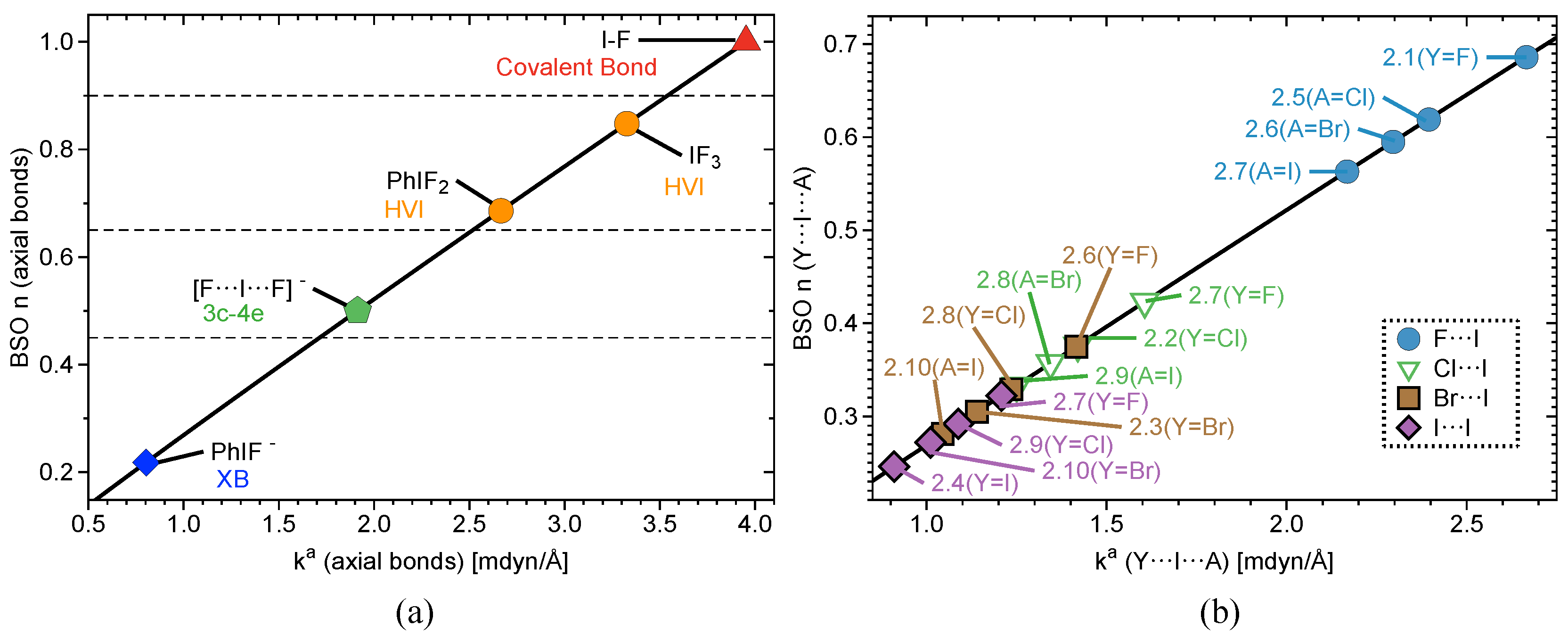
Interatomic distances (r), , , , BSO values, and local mode frequencies () are summarized in Table 1 and Table 2. Figure 2, Figure 3 and Figure 4 show the power relationship between BSO n and for Group 1, Y⋯IA and YI⋯A in Groups 2–4, where YI⋯A is weaker than Y⋯IA, and I–C equatorial (Ph, F, benzene) bonds in Groups 1–4. Note: in Table 1, the F⋯I interactions in 3.9 and 4.1 are the stronger bonds. These are the only two cases in Groups 3–4 where the halogen⋯I interaction is the stronger interaction. Therefore, CN and OCO will be considered A and F will be considered Y in Table 1 for these two cases only. However, this convention is not used for the BSO plots in Figure 3 and Figure 5. In these two figures, the Y⋯IA interaction is the bond between the non-halogen and I, and YI⋯A is the bond between the halogen and I. Figure 2a is a BSO plot for interactions in 1.1–2.1. Comparing bond strength in axial I–F interactions in FI, IF, PhIF, IF, and PhIF reveals the hypothesized trend: FI > IF (3c–4e HVIB) > PhIF (3c–4e HVIB) > IF (3c–4e) > PhIF (XB). As expected, the 2c–2e FI bonds in 1.1 and 1.4 are stronger than 3c–4e in 1.2 and 1.4. The latter are stronger than the I⋯F XB in 1.3, as shown in Table 1 and Figure 2. It is notable that the hypervalent IF forms a shorter and stronger 2c–2e bond compared to the FI molecule. Axial F atoms pull charge from iodine, resulting in a more polar 2c–2e I–F bond, and also contract the I orbital, improving I–F orbital overlap. The 3c–4e bond in IF is stronger than that of PhIF because the equatorial F polarizes the central I, causing more polar and stronger interactions at the axial positions. The equatorial Ph and benzene groups do not have the polarizing ability of F, but they do bind strongly to (BSO n = 0.648–1.046) and pull charge from the central I. The effect of the equatorial ligand causes the difference in bond strength between PhIF and IF. IF has no equatorial ligand and less polar bonds than the 3c–4e bond in PhIF. When replacing a F with a Ph group (1.3), the negative charge becomes localized in the fluorine due to its higher electronegativity; as a result, two different types of bond are formed: one is the 2c–2e C–I bond, and the other is an XB between I and F (the lower polarizing power of Ph results in a less positive charge at the iodine).
Figure 2b shows Y⋯I⋯A (where A = F, Cl, Br, and I in this case) in 2.1–2.10. In the case of PhIY (2.1–2.4), there is a correlation between bond strength and bond polarity. Charge on the central I atom increases in the series: PhI< PhIBr< PhICl< PhIF. This matches the trend in 3c–4e bond strength. Charge on the axial ligand also matches this order, but with charge becoming more negative. In 2.5–2.10, there is a marked difference in I⋯F bond strength (BSO n> 0.562) and all other axial bonds (BSO n = 0.272–0.423). I⋯Cl, I⋯Br, and I⋯I interactions are similar in bond strength, but vary slightly depending on the atom on the opposite side of the 3c–4e bond. This result is in accord with observed bond polarity and electronegativity trends of halogens.
Figure 3a shows BSO plots for Y⋯IA and Figure 3b YI⋯A in Groups 3–4. The same trend emerges again when replacing one halogen with an electron-donating functional group; the bond strength of I⋯A increases when A changes from I to F. Keeping the Y constant and substituting A again reproduce the trend that bonds become stronger when going up the periodic table from I to F for all five functional groups. When comparing the functional groups, bond strength follows this order: OCO > OC(CH)> OH > CN > NH. This order holds regardless of the axial halogen. This pattern nearly matches the order observed in group charges where the more negatively-charged the group, the higher the BSO . The exception is OH and OC(CH). OH groups are more negatively charged, but do not bind as strongly as OC(CH) groups. This is because the benzene in 4.5–4.8 binds more strongly on average in Group 4 (BSO n = 0.898–1.046) than Ph in Group 2 (BSO n = 0.691–0.914) and Ph in Group 3 (BSO n = 0.648–0.893). The stronger equatorial bond correlates to a more positive charge on the central I, which allows for stronger 3c–4e bonds. The key difference between Group 4 and Groups 2–3 is that all of Group 4 has functional groups bound directly to benzene and Groups 2–3 do not. In this case, it is justifiable to state that the C(CH) group in 4.5–4.8 will be an electron donor to benzene, which accounts for the lower group charge. 2.1 and 3.8 are the only exceptions to this trend.
2.3. Covalent/Electrostatic Contributions
Figure 4b and Figure 5 contain three plots correlating BSO with of I⋯axial halogens in Group 2 (Figure 4b), Y⋯IA in Groups 3–4 (Figure 5a), and YI⋯A in Groups 3–4 (Figure 5b). The vertical dashed line through the origin separates the covalent region from the electrostatic region according to the Cremer–Kraka criterion. < 0 for every I–A, I–Y, and I–C equatorial (Ph, F, or benzene) interaction, putting them in the covalent bonding region or very close to the electrostatic region in some cases. There is significant covalent contribution for the axial bonding interactions in 2.1–4.8, indicating that charge accumulation in the bonding region produces a net stabilizing effect. For the plot in Figure 4b, there is a good linear correlation between BSO n and , as indicated by a value of = 0.930. These data correlate higher bond strength to an increase in covalent character of the interaction. The weaker the bond, the closer to the electrostatic region. The plot is sectioned off into regions to show agreement with Figure 2a. The XB interaction in PhIF is at the bottom of the plot, closest to the electrostatic region. The 3c–4e region is next, where IF is found, along with all of the weakly-bound -iodanes containing axial Cl, Br, and I atoms. It is necessary to note that we expect the 3c–4e bond in IF to be the strongest of all trihalides and to be at the very top of the spectrum. Therefore, if considering other trihalide systems, one would expect to see better separation between 3c–4e bonds in HVI and 3c–4e bonds in trihalides, as is observed for the more closely-related IF, PhIF, and IF. All of the -iodanes containing F are at the very top of this region bordering the next region or in the next region, which is 3c–4e HVI. IF and PhIF give prime examples of the 3c–4e HVIB. At the very top right corner is the covalent F–I complex. As we follow the linear data from the weak electrostatic region to the strong covalent region, we once again reproduce the smooth continuum: partially-covalent XB < 3c–4e bond in trihalides < 3c–4e bond in HVI < covalent bond. Now, the trend holds in terms of covalent/electrostatic character and . Note that in Figure 4 and Figure 5, could be plotted against BSO in place of , and the same correlation would occur, but with a positive slope instead of a negative one.
The same general trend is observed in Figure 5 for Groups 3–4. As BSO n increases, becomes more negative (deeper into the covalent region). In Figure 5a, points for Y⋯I are scattered, and the correlation weakens when taking the data as a whole. However, if considering each functional group individually, a strong linear correlation once again occurs. The periodic trend emerges that as A, the halogen homolog becomes smaller, the bond strengthens and becomes more covalent in nature. This is not a direct result of the axial ligand, rather it is the result of the polarizing effect the axial halogen has on the central I atom. The Y⋯IA interactions (< –0.237 Hartree/Å) sit significantly farther into the covalent region compared to the YI⋯A interactions (< –0.055 Hartree/Å). Figure 5b again shows a reasonable linear correlation with R = 0.917. The trend amongst functional groups previously noted in 3.1–3.2 is once again evident here: OCO > OC(CH)> OH > CN > NH in terms of pulling charge from the central I, which results in strengthening and to some degree increasing of the I⋯A bond. Another important point here is that one must not assume certain functional groups will behave the same way in all situations as they behave when bound to benzene. A prime example is CN: a strong electron withdrawing group (when bound to benzene) is the second weakest withdrawing group in this study.
2.4. 3c–4e Bonding
%3c–4e bonding character is shown Table 1. Vibrational spectroscopy was utilized to define a new and simple 3c–4e parameter, which was derived from Local Mode Analysis (L-modes). It utilizes BSO values to define %3c–4e bonding as:
where BSO n (Y⋯I) > BSO n (A⋯I). A⋯I is the weaker, less covalent bond, and Y⋯I is the stronger, more covalent bond. In 2.1–2.4, A = Y; therefore, 3c–4e is 100%. In 2.5–2.7, %3c–4e decreases from 68% in 2.5 to 57% in 2.7 as BSO n becomes larger. 2.8–2.10 contain weakly-bound halogens, which promote high 3c–4e bonding character (88–97%). In 3.1–3.12, there is a large range of 3c–4e contributions to the Y⋯I⋯A interactions (45–94%). The highest percentage is in 3.5, where the 3c–4e interaction is HO⋯I⋯F. Both substituents have lp electrons and are highly electronegative. The bonds formed are strong and polar, as the central I is the most polarized of all Group 3 molecules with an NBO charge of +1.401 e. OH and F have similar BSO and NBO charges: n = 0.625, −0.565 e and n = 0.590, −0.703 e, respectively. The 3.1 has high 3c–4e character for the same reason as 3.5, but with NH involved instead of OH. N is slightly less electronegative than O, and NH has a more positive charge than OH, and thus forms a slightly weaker, less polar bond. 3.3–3.4 and 3.7–3.8 have the lowest 3c–4e character in Group 3. These species contain mostly I–Br or I–I bonds, which bind weakly, while on the other side of the Y⋯I⋯A, we have polar functional groups OH and NH. There is a strong polar interaction on one side of I and a weak non-polar interaction on the other side, which decreases the 3c–4e character. 4.1–4.4 have high 3c–4e character (81–85%). The I–O oxygen is part of an ester group which carries a large negative charge and contributes resonance stabilization. In 4.5–4.8, I is bound to the O on a T-butoxy group, which is slightly less electron rich and does not have the benefit of resonance. The T-butoxy-O binds strongly to I compared to Cl, Br, and I.
3. Computational Methods
DFT was utilized to optimize molecular geometries and to calculate for each stationary point molecular vibrational frequencies including the L-modes of Konkoli and Cremer [60,61,62] and the determination of local mode force constants (), NBO charges, electron densities , and energy densities ; where is a bond critical point. Each stationary point was confirmed as a minimum by absence of imaginary normal mode frequencies. Available experimental geometries for the ICl dimer, IF, IF, dichloroiodobenzene (PhICl), and diacetoxyiodobenzene (PhI(OAc)) [18,63,64,65,66] were used to gauge the accuracy of the DFT calculations. Experimental and calculated geometries using different model chemistries for this set of compounds are compared in Table A1 and Table A2 (See Appendix A). We initially employed Grimme’s Rung 5 double hybrid density functional B2PLYP [67] and Dunning’s cc-pVDZ basis set [68,69,70,71] with a tight convergence criterion and an ultra-fine integration grid. The B2PLYP functional combines the generalized gradient approximation exchange functional of Becke [72,73] and the Lee–Yang–Parr correlation functional [74] with exact Hartree–Fock exchange and Møller–Plesset perturbation theory [75,76,77,78] of second order (MP2) [79,80,81]. This functional has shown close agreement between calculated and experimental geometries and vibrational frequencies for heavy atoms [82,83]. However, for our set of molecules, the cc-pVDZ basis set did not produce the desired accuracy (Table A1 and Table A2), and the B2PLYP/aug-cc-pVTZ level of theory became computationally expensive. The combination of MP2 and a relatively small double-zeta basis set is known to provide a fortuitous cancellation of error [84,85]. MP2 overestimates correlation energy, but this is compensated by the cc-pVDZ basis set [86]. Therefore, we tested MP2/cc-pVDZ for reducing the computer time. However, results calculated at this level of theory gave less accurate results than B97X-D/aug-cc-pVTZ [87,88], while calculations at the B2PLYP/Def2TZP level of theory led to inaccurate results in several cases. For Br and I, scalar relativistic effects were assessed by using effective core potentials (ECPs) in combination with the Dunning basis sets [89,90].
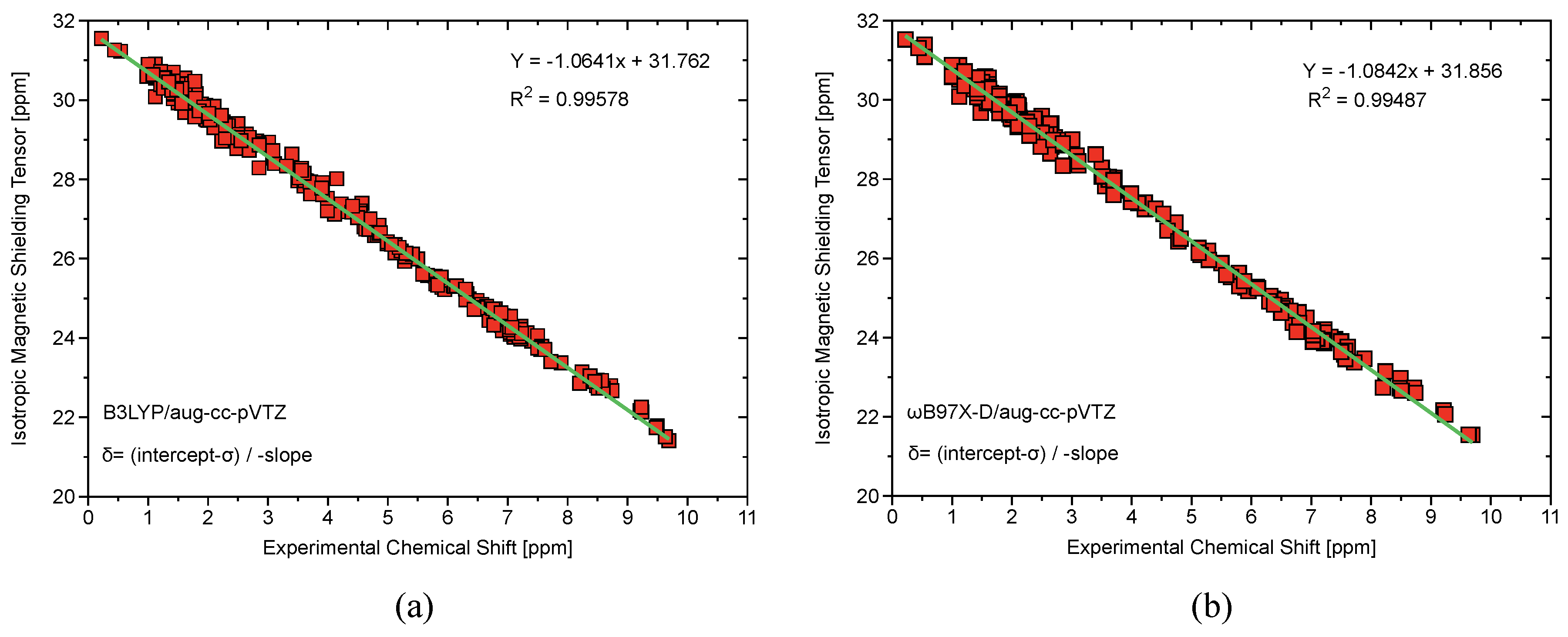
Although geometries are first order properties and therefore less sensitive to the level of theory, B2PLYP/aug-cc-pVTZ and B97X-D/aug-cc-pVTZ calculations turned out to be in closest agreement with experimental data, while for a small subset of compounds, close agreement between B97X-D/aug-cc-pVTZ and CCSD(T)/aug-cc-pVTZ was obtained (Table A3). To further rationalize these results, gauge-independant atomic orbital (GIAO) magnetic shielding tensors [91,92,93,94,95] were calculated and isotropic shielding constants were converted into chemical shifts utilizing the linear regression method of Tantillo et al. for PhICl, PhI(OAc), and 1-Hydroxy-1,2-benziodoxol-3(1H)-one [96,97,98,99,100,101]. This method requires the calculation of isotropic magnetic shielding tensors for a test set of molecules at a given level of theory (in our case, B97X-D/aug-cc-pVTZ and B3LYP/aug-cc-pVTZ), plotting the raw calculated isotropic value against experimental NMR chemical shifts, and using the following relationship to develop an equation for calculating chemical shifts (Figure A1):
where is the derived chemical shift and is the calculated isotropic magnetic shielding tensor. The margin of error for proton-NMR chemical shifts turned out to be 0.24–6.91% for the B3LYP functional and 0.19–5.81% for the B97X-D functional (Table A4) [18,63,102]. Although both B97X-D and B3LYP gave satisfactory and similar calculated chemical shifts, B97X-D gave more accurate geometries and frequencies.
Based on these findings, the B97X-D/aug-cc-pVTZ level of theory was chosen for this study due to its displayed ability to predict accurate first and second order experimental properties in HVI molecules in addition to the previous findings of Oliveira et al. that this level of theory is suitable for the detailed analysis of XB [41].
Vibrational spectroscopy was applied to quantify the intrinsic strength of HVIBs. Chemists have utilized vibrational spectroscopy to obtain information about the electronic structure of molecules and their framework of bonds. However, normal vibrational modes cannot be used as a direct bond strength measure because they are delocalized due to electronic and mass coupling, a fact that often has been overlooked [103,104]. The electronic coupling is eliminated by solving the Wilson equation of spectroscopy [105] and transforming to normal coordinates. Konkoli and Cremer showed that the remaining mass (kinematic) coupling can be eliminated by solving a mass-decoupled equivalent of the Wilson equation, leading to local vibrational modes, which are associated with internal coordinates such as bond lengths, bond angles, and dihedral angles [60,106]. Zou and Cremer verified that there is a one-to-one relationship between local and normal vibrational modes through an adiabatic connection scheme (ACS) [107,108,109], allowing a normal mode decomposition into local mode contributions [44,110,111] and, as such, the detailed analysis of a vibrational spectrum. This is of particular value, given the fact that L-modes can be applied to both calculated and measured spectra [61,112].
Another important feature of L-modes is the direct relationship between the local stretching force constant () of a chemical bond and its intrinsic strength [113]. This has enhanced our knowledge about chemical bonding and the often overlooked, but highly important weak intermolecular interactions, providing a wealth of new insight into: (i) covalent bonding [113], stretching from peculiar cases of reversed bond length-bond strength relationships [114,115], to a new design recipe for fluorinating agents [116]; (ii) weak chemical interactions including hydrogen bonding [117,118], XB [35,41,42], pnicogen bonding [43], chalcogen bonding [50], weak interactions in gold clusters [119], as well as non-classical hydrogen bonds in boron–hydrogen interactions [120,121]. In addition, new electronic parameters and rules were derived [122,123,124].
When comparing a larger set of , the use of a relative bond strength order (BSO ) is convenient [103,104]. The BSO of a bond is obtained by utilizing the extended Badger rule [103,104,125] according to which BSO n is related to by a power relationship, which is fully determined by two reference values and the requirement that for a zero-force constant, the BSO value becomes zero:
The constants a and b are calculated from values of two reference compounds with known BSO values n and n via:
and,
In this work, we chose as reference compounds FI and IF representing BSO values of one and 0.5, respectively, guided by the corresponding Mayer bond orders [126] of 0.940 and 0.543 evaluated at the B97X-D/cc-pVTZ level of theory. More than 50% of iodine bonds in this work include an atom from the second period. This renders the FI/IF reference system ideal (a second period atom bound to iodine), in addition to providing a spectrum with a full 3c–4e bond from a trihalide (IF) on the one end and a full covalent bond (FI) on the other end.
Using the of 1.913 mdyn/Å for IFand 3.953 mdyn/Å for FI (B97X-D/cc-pVTZ level of theory), the constants a and b in the power relationship Equation (3) were determined to be a = 0.269 and b = 0.955, leading to:
Because the chosen reference system was designed for 3c–4e interactions particular to this study, a scaling procedure was used to obtain appropriate BSO values for covalent I–C interactions between the equatorial ligands and the central iodine. The equatorial bonds are fully-formed single bonds, but the C–I bond is much less polar and weaker than the I–F bond used as a reference. We calculated = 2.557 mdyn/Å for the I–C bond in iodobenzene. From Equation (6), we calculated BSO = 0.659. The scaling factor was obtained by setting n = 1 for this I–C bond. The scaling factor is 1/0.659 = 1.517, which was applied to BSO of all equatorial I–C bonds. Multiplying the scaling factor through Equation (6) provided a new BSO equation for assessing the strength of the equatorial I–C bonds in this study:
The Cremer–Kraka criterion was applied to assess the covalent nature of HVIB [42,55,56,77,127]. According to this criterion, a covalent bond between two atoms A and B is defined by (1) the existence of a zero-flux surface and bond critical point between atoms A and B (necessary condition) and (2) a negative and thereby stabilizing local energy density (sufficient condition). will be close to zero or positive if the interaction between A and B is non-covalent, that is electrostatic or of the dispersion type. is defined as:
where is the kinetic energy density (always positive, destabilizing) and is the potential energy density (always negative, stabilizing). In addition to the established Cremer–Kraka criterion, a molecular fragmentation scheme for estimating electron density shifts has recently emerged as a potential tool for the qualitative investigation of non-covalent interactions at low computational cost [128].
L-modes was carried out with the program COLOGNE2018 [129], and Mayer bond orders were determined with the program ORCA [130]. NBO populations were computed using NBO 6 [131,132,133,134]. The electron density analysis, in particular the calculation of electron density at the bond critical point () and , was performed with the program AIMAll [135,136]. All DFT calculations were carried out with GAUSSIAN16 [137].
4. Conclusions
In this work, we quantified the intrinsic bond strength and bonding nature of a series of HVI compounds through vibrational spectroscopy. Use of DFT in this work was rationalized by testing several levels of theory against first and second order experimental properties of a small set of known HVI reagents. The computed set of 34 HVI molecules was then compared to XB, 3c–4e bonding, and covalent bonding in terms of BSO , , , , and NBO charges. Recently, Politzer and coworkers [138] showed that by substituting a ligand in trihalides with a negative point charge, the positive electrostatic potential at the polarized -hole collinear to the point charge correlates qualitatively well with the interaction energy; substantiating the key role played by electrostatics, which is also reflected in the atomic charge distribution (see Figure 1) and can be rationalized in terms of the 3c–4e model. The more negative charge at the ligands Y and A compared to the central iodine is due to the presence of a node at the center of the occupied non-bonding orbital [139]. This charge separation is responsible for the lower covalent character of 3c–4e bonds compared to a classical 2c–2e bond. Politzer and coworkers proposed the existence of a continuum between non-covalent and covalent bonds, the latter being a result of an increased degree of polarization [138]. Our results do also suggest the existence of such a continuum, but whether covalency can be seen as a degree of polarization is still disputable, especially in view of Ruedenberg’s description of covalent bonding, where energy lowering is a result of the complex interplay of kinetic and potential energy contributions [140,141]. The 3c–4e bonds in HVI share properties with XB, but are more closely related to the 3c–4e bonds in trihalides or covalent bonding in extreme cases. The equatorial 2c–2e HVI bond is stronger than comparable 3c–4e bonds (bonds involving the same ligands like in IF) and is more closely related to a covalent bond. Our results support the following transition: XB < 3c–4e bond in trihalides < 3c–4e bond in HVI < 2c–2e bond in PhIF< covalent bond. When comparing the difference (equatorial ligands) between trihalides and -iodanes, we found that the 3c–4e HVIB is strengthened by the equatorial ligand by comparing IF, PhIF, and IF. The equatorial ligand contributes significantly in pulling electron density from the central I, allowing for more polar interactions. Thus, highly electronegative ligands at the equatorial position will form strong interactions, as will axial ligands in such a case. We also found that axial ligands in HVIs have a minimal direct effect on one another in terms of NBO charge analysis, but do play a role in altering charge on the central I. Substituent effects in HVI can alter bond strength in both axial ligands and the equatorial ligand, particularly when F atoms are involved as ligands. The five functional groups studied here play a bond-strengthening and -polarizing role in the following order: OCO > OC(CH)> OH > CN > NH, with OH and OC(CH) being partially interchangeable. In terms of , we found a strong linear correlation with BSO n. becoming more negative correlates to an increase in bond strength. Furthermore, large stabilization in the bonding region correlates to the increased covalent character of a bond. Finally, we found the 3c–4e bond concept to be a valuable descriptor in terms of the linear portion of -iodanes.
Future goals are to utilize L-modes and the analysis of the electrostatic potential to explain why the T-shaped molecular geometry in -iodanes contains improper dihedrals and non-ideal bond angles. We also plan to investigate 3c–4e bonding and intramolecular HB in a series of HVI reagents utilizing L-modes and to explore the chemical reactivity of HVI compounds utilizing the unified reaction valley approach developed in our group [103,142,143,144]. In addition, we will perform a conformational and geometrical study of a series of novel HVI monomeric materials with a strong potential of forming useful polymers [145,146].
Author Contributions
Conceptualization, S.Y., V.O., and E.K.; methodology, E.K.; formal analysis, S.Y. and V.O.; investigation, S.Y. and V.O.; data curation, S.Y. and V.O.; software and programming, N.V.; writing, original draft preparation, S.Y. and V.O.; writing, review and editing, E.K.; visualization, S.Y. and V.O.; supervision, E.K.
Funding
This research was funded by the National Science Foundation Grant Number CHE 1464906 and the Brazilian Grant Number 2018/13673-3 São Paulo Research Foundation (FAPESP).
Acknowledgments
We thank Southern Methodist University for providing excellent computational resources. We also thank Nicolay Tsarevsky for introducing the interesting field of HVI compounds to us and Marek Freindorf for technical support and assistance with methodology questions.
Conflicts of Interest
The authors declare no conflict of interest.
Appendix A
Table A1 shows bond lengths, bond angles, and % error compared to experimentally measured data for IF, IF, and (ICl). For each molecule, geometry optimizations and vibrational frequencies were calculated at the B2PLYP/cc-pVDZ, B2PLYP/aug-cc-pVTZ, B2PLYP/Def2TZP, B3LYP/aug-cc-pVTZ, B97X-D/aug-cc-pVTZ, and M2P/cc-pVDZ levels of theory. B2PLYP/aug-cc-pVTZ and B97X-D/aug-cc-pVTZ levels of theory give superior results for the given geometry parameters. Table A2 shows bond lengths, bond angles, and % error compared to experimentally measured data for PhICl and PhI(OAc) computed at all of thee aforementioned levels of theory. These two molecules are similar, or the same in the case of PhICl as the majority of the molecules in this work. The B97X-D/aug-cc-pVTZ gave remarkable accuracy in calculating geometry parameters for these two molecules.

Table A1.
Calculated and experimental bond lengths and bond angles for the (ICl) dimer, IF, and IF, showing B2PLYP and B97X-D/aug-cc-pVTZ levels of theory giving closest agreement with the experiment [64,65,66].
| Method | r (I–Cl, F) | % | r (I–Cl, F) | % | % | |
|---|---|---|---|---|---|---|
| Basis Set | [Å] | Error | [Å] | Error | Degrees | Error |
| (ICl)B2PLYP | ||||||
| cc-pVDZ | 2.432 | 1.97 | 2.770 | 1.83 | N/A | N/A |
| aug-cc-pVTZ | 2.397 | 0.50 | 2.733 | 0.48 | N/A | N/A |
| Def2TZP | 2.448 | 2.64 | 2.773 | 1.95 | N/A | N/A |
| B3LYP | ||||||
| aug-cc-pVTZ | 2.412 | 1.13 | 2.758 | 1.40 | N/A | N/A |
| B97X-D | ||||||
| aug-cc-pVTZ | 2.364 | 0.88 | 2.744 | 0.88 | N/A | N/A |
| MP2 | ||||||
| cc-pVDZ | 2.420 | 1.47 | 2.746 | 0.96 | N/A | N/A |
| Experiment | 2.385 | N/A | 2.720 | N/A | N/A | N/A |
| IF | ||||||
| B2PLYP | ||||||
| cc-pVDZ | 1.900 | 3.04 | 1.941 | 3.85 | N/A | N/A |
| aug-cc-pVTZ | 1.847 | 0.16 | 1.908 | 2.09 | N/A | N/A |
| Def2TZP | 1.859 | 0.81 | 1.919 | 2.68 | N/A | N/A |
| B3LYP | ||||||
| aug-cc-pVTZ | 1.857 | 0.70 | 1.918 | 2.62 | N/A | N/A |
| B97X-D | ||||||
| aug-cc-pVTZ | 1.840 | 0.22 | 1.901 | 1.71 | N/A | N/A |
| MP2 | ||||||
| cc-pVDZ | 1.895 | 2.77 | 1.933 | 3.42 | N/A | N/A |
| Experiment | 1.844 | N/A | 1.869 | N/A | N/A | N/A |
| IF | ||||||
| B2PLYP | ||||||
| cc-pVDZ | 1.931 | 3.15 | 1.984 | 0.05 | 169.2 | 5.55 |
| aug-cc-pVTZ | 1.885 | 0.69 | 1.960 | 1.16 | 167.7 | 4.61 |
| Def2TZP | 1.900 | 1.50 | 1.975 | 0.40 | 168.6 | 5.18 |
| B3LYP | ||||||
| aug-cc-pVTZ | 1.900 | 1.50 | 1.975 | 0.40 | 168.6 | 5.18 |
| B97X-D | ||||||
| aug-cc-pVTZ | 1.876 | 0.21 | 1.951 | 1.61 | 167.5 | 4.49 |
| MP2 | ||||||
| cc-pVDZ | 1.925 | 2.83 | 1.977 | 0.30 | 168.2 | 4.93 |
| Experiment | 1.872 | N/A | 1.983 | N/A | 160.3 | N/A |
Table A2.
Calculated and experimental bond lengths and bond angles for PhICl and PhI(OAc) showing B2PLYP/aug-cc-pVTZ and B97X-D/aug-cc-pVTZ levels of theory giving closest agreement with the experiment [18,63].
| Method | r (I–Cl, O) | % | r (I–C) | % | % | |
|---|---|---|---|---|---|---|
| Basis Set | [Å] | Error | [Å] | Error | Degrees | Error |
| PhICl | ||||||
| B2PLYP | ||||||
| cc-pVDZ | 2.536 | 2.26 | N/A | N/A | 90.5 | 1.46 |
| aug-cc-pVTZ | 2.505 | 1.01 | N/A | N/A | 89.6 | 0.45 |
| Def2TZP | 2.558 | 3.15 | N/A | N/A | 89.8 | 0.67 |
| B3LYP | ||||||
| aug-cc-pVTZ | 2.524 | 1.77 | N/A | N/A | 90.3 | 1.23 |
| B97X-D | ||||||
| aug-cc-pVTZ | 2.481 | 0.04 | N/A | N/A | 89.2 | 0.00 |
| MP2 | ||||||
| cc-pVDZ | 2.517 | 1.49 | N/A | N/A | 88.9 | 0.34 |
| Experiment | 2.480 | N/A | N/A | N/A | 89.2 | N/A |
| PhI(OAc) | ||||||
| B2PLYP | ||||||
| cc-pVDZ | 2.212 | 2.60 | 2.150 | 2.87 | 164.5 | 0.30 |
| aug-cc-pVTZ | 2.178 | 1.02 | 2.081 | 0.43 | 162.8 | 0.73 |
| Def2TZP | 2.179 | 1.07 | 2.111 | 1.00 | 163.1 | 0.55 |
| B3LYP | ||||||
| aug-cc-pVTZ | 2.194 | 1.76 | 2.124 | 1.63 | 163.7 | 0.18 |
| B97X-D | ||||||
| aug-cc-pVTZ | 2.149 | 0.32 | 2.104 | 0.67 | 162.9 | 0.66 |
| MP2 | ||||||
| cc-pVDZ | 2.187 | 1.44 | 2.122 | 1.53 | 162.7 | 0.79 |
| Experiment | 2.156 | N/A | 2.090 | N/A | 164.0 | N/A |
Table A3 compares computed bond lengths and for FI, IF, IF, and IF at the B97X-D/CCSD(T)/aug-cc-pVTZ level of theory. Once again, B97X-D/aug-cc-pVTZ performs remarkably well compared to the gold standard CCSD(T). Table A4 shows calculated and experimental NMR shifts for PhICl, PhI(OAc), and 1-hydroxy-1,2-benziodoxol-3(1H)-one using the B3LYP and 97X-D functionals with the aug-cc-pVTZ basis set. Figure A1 shows a strong linear correlation between calculated isotropic magnetic stretching tensors and experimentally measured chemical shifts. The calculations done at the B97X-D/aug-cc-pVTZ level of theory are slightly more in agreement with experimental measurements than the B3LYP/aug-cc-pVTZ.
Table A3.
Calculated r and of all FI bonds in FI, IF, IF3, and IF5 computed at the B97X-D/CCSD(T)/aug-cc-pVTZ level of theory.
Table A3.
Calculated r and of all FI bonds in FI, IF, IF3, and IF5 computed at the B97X-D/CCSD(T)/aug-cc-pVTZ level of theory.
| Molecule | r (FI) Equatorial | (FI) Equatorial | r (FI) Axial | (FI) Axial |
|---|---|---|---|---|
| Level of Theory | (Å) | (mdyn/Å) | (Å) | (mdyn/Å) |
| FI | ||||
| B97X-D/aug-cc-pVTZ | 1.921 | 3.953 | - | - |
| CCSD(T)/aug-cc-pVTZ | 1.931 | 3.705 | - | - |
| [F⋯I⋯F] | ||||
| B97X-D/aug-cc-pVTZ | 2.089 | 1.913 | - | - |
| CCSD(T)/aug-cc-pVTZ | 2.085 | 1.746 | - | - |
| IF | ||||
| B97X-D/aug-cc-pVTZ | 1.876 | 4.087 | 1.951 | 3.327 |
| CCSD(T)/aug-cc-pVTZ | 1.878 | 4.278 | 1.950 | 3.325 |
| IF | ||||
| B97X-D/aug-cc-pVTZ | 1.840 | 4.529 | 1.901 | 3.634 |
| CCSD(T)/aug-cc-pVTZ | 1.840 | 4.706 | 1.895 | 3.834 |
Table A4.
Calculated and experimental NMR chemical shifts for PhICl, PhI(OAc), and 1-hydroxy-1,2-benziodoxol-3(1H)-one computed using the aug-cc-pVTZ basis set [18,63,102].
| B97X-D | B3LYP | |||||
|---|---|---|---|---|---|---|
| Magnetic Isotropic | -Calculated | -Experimental | % | Magnetic Isotropic | -Calculated | % |
| Shielding Tensor | (ppm) | (ppm) | Error | Shielding Tensor | (ppm) | Error |
| PhICl | ||||||
| 23.64 | 7.58 | 7.16 | 5.51 | 23.77 | 7.51 | 4.65 |
| 23.57 | 7.65 | 7.40 | 3.24 | 23.71 | 7.57 | 2.19 |
| 23.41 | 7.79 | 7.68 | 1.42 | 23.57 | 7.70 | 0.24 |
| PhIOAc | ||||||
| 23.42 | 7.79 | 8.24 | 5.81 | 23.56 | 7.71 | 6.91 |
| 23.50 | 7.70 | 7.68 | 0.37 | 23.67 | 7.61 | 0.91 |
| 23.59 | 7.62 | 7.58 | 0.59 | 23.74 | 7.54 | 0.44 |
| 29.68 | 2.01 | 1.92 | 4.72 | 29.64 | 2.00 | 4.02 |
| 1-Hydroxy-1,2 | ||||||
| -benziodoxol-3(1H)-one | ||||||
| 23.45 | 7.76 | 7.71 | 0.58 | 23.61 | 7.66 | 0.65 |
| 22.91 | 8.26 | 8.02 | 2.85 | 23.04 | 8.20 | 2.19 |
| 23.20 | 7.99 | 7.97 | 0.19 | 23.36 | 7.90 | 0.90 |
| 23.30 | 7.89 | 7.85 | 0.50 | 23.44 | 7.82 | 0.35 |
Figure A1.
(a) Computed at the B3LYP/aug-cc-pVTZ level of theory, isotropic magnetic shielding tensors plotted against experimental NMR chemical shifts showing strong linear correlation and a slope close to -1 which is indicative of minimization of systematic error. (b) Computed at the B97X-D/aug-cc-pVTZ level of theory, isotropic magnetic shielding tensors plotted against experimental NMR chemical shifts again showing strong linear correlation and slope close to -1.

References
- Kieltsch, I.; Eisenberger, P.; Togni, A. Mild Electrophilic Trifluoromethylation of Carbon- and Sulfur-Centered Nucleophiles by a Hypervalent Iodine(III)–CF3 Reagent. Angew. Chem. Int. 2007, 46, 754–757. [Google Scholar] [CrossRef] [PubMed]
- Silva, F.C.S.; Tierno, A.F.; Wengryniuk, S.E. Hypervalent Iodine Reagents in High Valent Transition Metal Chemistry. Molecules 2017, 22, 780. [Google Scholar] [CrossRef]
- Charpentier, J.; Früh, N.; Togni, A. Electrophilic Trifluoromethylation by Use of Hypervalent Iodine Reagents. Chem. Rev. 2014, 115, 650–682. [Google Scholar] [CrossRef] [PubMed]
- Maddox, V.H.; Godefroi, E.F.; Parcell, R.F. The Synthesis of Phencyclidine and Other 1-Arylcyclohexylamines. J. Med. Chem. 1965, 8, 230–235. [Google Scholar] [CrossRef] [PubMed]
- Moriarty, R.M.; Enache, L.A.; Zhao, L.; Gilardi, R.; Mattson, M.V.; Prakash, O. Rigid Phencyclidine Analogues. Binding to the Phencyclidine and σ1 Receptors. J.Med. Chem. 1998, 41, 468–477. [Google Scholar] [CrossRef]
- Berger, G.; Soubhye, J.; Meyer, F. Halogen bonding in polymer science: From crystal engineering to functional supramolecular polymers and materials. Polym. Chem. 2015, 6, 3559–3580. [Google Scholar] [CrossRef]
- Murphy, G.K.; Racicot, L.; Carle, M.S. The Chemistry between Hypervalent Iodine(III) Reagents and Organophosphorus Compounds. Asian J. Org. Chem. 2018, 7, 837–851. [Google Scholar] [CrossRef]
- Ghosh, S.; Pradhan, S.; Chatterjee, I. A survey of chiral hypervalent iodine reagents in asymmetric synthesis. Beilstein J. Org. Chem 2018, 14, 1244–1262. [Google Scholar] [CrossRef] [Green Version]
- Cavallo, G.; Metrangolo, P.; Milani, R.; Pilati, T.; Priimagi, A.; Resnati, G.; Terraneo, G. The Halogen Bond. Chem. Rev. 2016, 116, 2478–2601. [Google Scholar] [CrossRef] [PubMed] [Green Version]
- Wulfsberg, G. Inorganic Chemistry; University Science Books: Sausalito, CA, USA, 2000. [Google Scholar]
- Crabtree, R.H. Hypervalency, secondary bonding and hydrogen bonding: Siblings under the skin. Chem. Soc. Rev. 2017, 46, 1720–1729. [Google Scholar] [CrossRef]
- Berger, G.; Soubhye, J.; van der Lee, A.; Vande Velde, C.; Wintjens, R.; Dubois, P.; Clément, S.; Meyer, F. Interplay between Halogen Bonding and Lone Pair-π Interactions: A Computational and Crystal Packing Study. ChemPlusChem 2014, 79, 552–558. [Google Scholar] [CrossRef]
- Labattut, A.; Tremblay, P.L.; Moutounet, O.; Legault, C.Y. Experimental and Theoretical Quantification of the Lewis Acidity of Iodine(III) Species. J. Org. Chem. 2017, 82, 11891–11896. [Google Scholar] [CrossRef] [PubMed]
- Kalescky, R.; Zou, W.; Kraka, E.; Cremer, D. Quantitative Assessment of the Multiplicity of Carbon-Halogen Bonds: Carbenium and Halonium Ions with F, Cl, Br, and I. J. Phys. Chem. A 2014, 118, 1948–1963. [Google Scholar] [CrossRef] [PubMed]
- Kalescky, R.; Kraka, E.; Cremer, D. Are carbon–halogen double and triple bonds possible? Int. J. Quant. Chem. 2014, 114, 1060–1072. [Google Scholar] [CrossRef]
- Yoshimura, A.; Zhdankin, V.V. Advances in Synthetic Applications of Hypervalent Iodine Compounds. Chem. Rev. 2016, 116, 3328–3435. [Google Scholar] [CrossRef] [PubMed]
- Zhdankin, V.V.; Stang, P.J. Chemistry of Polyvalent Iodine. Chem. Rev. 2008, 108, 5299–5358. [Google Scholar] [CrossRef] [PubMed] [Green Version]
- Archer, E.M.; van Schalkwyk, T.G. The crystal structure of benzene iododichloride. Acta. Crystallogr. A 1953, 6, 88–92. [Google Scholar] [CrossRef] [Green Version]
- Landrum, G.A.; Goldberg, N.; Hoffmann, R.; Minyaev, R.M. Intermolecular interactions between hypervalent molecules: Ph2IX and XF3 (X = Cl, Br, I) dimers. New J. Chem. 1998, 22, 883–890. [Google Scholar] [CrossRef]
- Bersuker, I.B. Modern Aspects of the Jahn–Teller Effect Theory and Applications To Molecular Problems. Chem. Rev. 2001, 101, 1067–1114. [Google Scholar] [CrossRef]
- Batsanov, S.S. Van der Waals Radii of Elements. Inorg. Mater. 2001, 37, 871–885. [Google Scholar] [CrossRef]
- Nyburg, S.C.; Faerman, C.H.; Prasad, L. A revision of van der Waals atomic radii for molecular crystals. II: Hydrogen bonded to carbon. Acta Crystallogr. B 1987, 43, 106–110. [Google Scholar] [CrossRef]
- Nyburg, S.C.; Faerman, C.H. A revision of van der Waals atomic radii for molecular crystals: N, O, F, S, Cl, Se, Br and I bonded to carbon. Acta Crystallogr. B 1985, 41, 274–279. [Google Scholar] [CrossRef] [Green Version]
- Ishikawa, M.; Ikuta, S.; Katada, M.; Sano, H. Anisotropy of van der Waals radii of atoms in molecules: Alkali-metal and halogen atoms. Acta Crystallogr. B 1990, 46, 592–598. [Google Scholar] [CrossRef]
- Badenhoop, J.K.; Weinhold, F. Natural steric analysis: Ab initio van der Waals radii of atoms and ions. J. Chem. Phys. 1997, 107, 5422–5432. [Google Scholar] [CrossRef]
- Bader, R.F.W.; Henneker, W.H.; Cade, P.E. Molecular Charge Distributions and Chemical Binding. J. Chem. Phys. 1967, 46, 3341–3363. [Google Scholar] [CrossRef]
- Bader, R.F.W.; Carroll, M.T.; Cheeseman, J.R.; Chang, C. Properties of atoms in molecules: Atomic volumes. J. Am. Chem. Soc. 1987, 109, 7968–7979. [Google Scholar] [CrossRef]
- Bader, R.F.W.; Bandrauk, A.D. Relaxation of the Molecular Charge Distribution and the Vibrational Force Constant. J. Chem. Phys. 1968, 49, 1666–1675. [Google Scholar] [CrossRef]
- Molina, J.M.; Dobado, J.A. The three-center-four-electron (3c–4e) bond nature revisited. An atoms-in-molecules theory (AIM) and ELF study. Theor. Chim. Acta. 2001, 105, 328–337. [Google Scholar] [CrossRef]
- Musher, J.I. The Chemistry of Hypervalent Molecules. Angew. Chem. Ed. 1969, 8, 54–68. [Google Scholar] [CrossRef]
- Reed, A.E.; von Ragué Schleyer, P. Chemical Bonding in Hypervalent Molecules. The Dominance of Ionic Bonding and Negative Hyperconjugation over d-orbital Participation. J. Am. Chem. Soc. 1990, 112, 1434–1445. [Google Scholar] [CrossRef]
- Magnusson, E. Hypercoordinate Molecules of Second-Row Elements: d Functions or d Orbitals? J. Am. Chem. Soc. 1990, 112, 7940–7951. [Google Scholar] [CrossRef]
- Landrum, G.A.; Goldberg, N.; Hoffmann, R. Bonding in the trihalides (X3−), mixed trihalides (X2Y−) and hydrogen bihalides (X2H−). The connection between hypervalent, electron-rich three-center, donor-acceptor and strong hydrogen bonding. Dalton Trans. 1997, 0, 3605–3613. [Google Scholar] [CrossRef]
- Yang, L.M.; Ganz, E.; Chen, Z.; Wang, Z.X.; von Ragué Schleyer, P. Four Decades of the Chemistry of Planar Hypercoordinate Compounds. Angew. Chem. Int. Ed. 2015, 54, 9468–9501. [Google Scholar] [CrossRef]
- Oliveira, V.; Kraka, E.; Cremer, D. The intrinsic strength of the halogen bond: Electrostatic and covalent contributions described by coupled cluster theory. Phys. Chem. Chem. Phys. 2016, 18, 33031–33046. [Google Scholar] [CrossRef]
- Wolters, L.P.; Bickelhaupt, F.M. Halogen Bonding versus Hydrogen Bonding: A Molecular Orbital Perspective. ChemistryOpen 2012, 1, 96–105. [Google Scholar] [CrossRef] [Green Version]
- Cozzolino, A.F.; Elder, P.J.; Vargas-Baca, I. A survey of tellurium-centered secondary-bonding supramolecular synthons. Coord. Chem. Rev. 2011, 255, 1426–1438. [Google Scholar] [CrossRef]
- Freindorf, M.; Kraka, E.; Cremer, D. A comprehensive analysis of hydrogen bond interactions based on local vibrational modes. Int. J. Quant. Chem. 2012, 112, 3174–3187. [Google Scholar] [CrossRef]
- Scheiner, S. Detailed comparison of the pnicogen bond with chalcogen, halogen, and hydrogen bonds. Int. J. Quantum Chem. 2012, 113, 1609–1620. [Google Scholar] [CrossRef] [Green Version]
- Scheiner, S. The Pnicogen Bond: Its Relation to Hydrogen, Halogen, and Other Noncovalent Bonds. Acc. Chem. Res. 2012, 46, 280–288. [Google Scholar] [CrossRef] [PubMed]
- Oliveira, V.; Kraka, E.; Cremer, D. Quantitative Assessment of Halogen Bonding Utilizing Vibrational Spectroscopy. Inorg. Chem. 2016, 56, 488–502. [Google Scholar] [CrossRef] [PubMed]
- Oliveira, V.; Cremer, D. Transition from metal–ligand bonding to halogen bonding involving a metal as halogen acceptor a study of Cu, Ag, Au, Pt, and Hg complexes. Chem. Phys. Lett. 2017, 681, 56–63. [Google Scholar] [CrossRef]
- Oliveira, V.; Kraka, E. Systematic Coupled Cluster Study of Noncovalent Interactions Involving Halogens, Chalcogens, and Pnicogens. J. Phys. Chem. A 2017, 121, 9544–9556. [Google Scholar] [CrossRef] [PubMed]
- Setiawan, D.; Kraka, E.; Cremer, D. Description of pnicogen bonding with the help of vibrational spectroscopy—The missing link between theory and experiment. Chem. Phys. Lett. 2014, 614, 136–142. [Google Scholar] [CrossRef]
- Setiawan, D.; Kraka, E.; Cremer, D. Strength of the Pnicogen Bond in Complexes Involving Group VA Elements N, P, and As. J. Phys. Chem. A 2014, 119, 1642–1656. [Google Scholar] [CrossRef] [PubMed]
- Tao, Y.; Tian, C.; Verma, N.; Zou, W.; Wang, C.; Cremer, D.; Kraka, E. Recovering Intrinsic Fragmental Vibrations Using the Generalized Subsystem Vibrational Analysis. J. Chem. Theory Comput. 2018, 14, 2558–2569. [Google Scholar] [CrossRef] [PubMed]
- Kraka, E.; Cremer, D. Dieter Cremer’s Contribution to the Field of Theoretical Chemistry. Int. J. Quantum Chem. 2019, 119, e25849. [Google Scholar] [CrossRef]
- Bene, J.D.; Alkorta, I.; Elguero, J. Halogen Bonding Involving CO and CS with Carbon as the Electron Donor. Molecules 2017, 22, 1955. [Google Scholar] [CrossRef]
- Alkorta, I.; Elguero, J.; Bene, J.E.D. Boron as an Electron-Pair Donor for B⋯Cl Halogen Bonds. ChemPhysChem. 2016, 17, 3112–3119. [Google Scholar] [CrossRef]
- Oliveira, V.; Cremer, D.; Kraka, E. The Many Facets of Chalcogen Bonding: Described by Vibrational Spectroscopy. J. Phys. Chem. A 2017, 121, 6845–6862. [Google Scholar] [CrossRef]
- Bene, J.E.D.; Alkorta, I.; Elguero, J. Hydrogen and Halogen Bonding in Cyclic FH(4-n):FCln Complexes, for n = 0–4. J. Phys. Chem. A 2018, 122, 2587–2597. [Google Scholar] [CrossRef] [PubMed]
- Cavallo, G.; Murray, J.S.; Politzer, P.; Pilati, T.; Ursini, M.; Resnati, G. Halogen bonding in hypervalent iodine and bromine derivatives: Halonium salts. IUCrJ 2017, 4, 411–419. [Google Scholar] [CrossRef]
- Heinen, F.; Engelage, E.; Dreger, A.; Weiss, R.; Huber, S.M. Iodine(III) Derivatives as Halogen Bonding Organocatalysts. Angew. Chem. Int. Ed. 2018, 57, 3830–3833. [Google Scholar] [CrossRef] [PubMed]
- Zhdankin, V.V. Hypervalent Iodine Chemistry: Preparation, Structure, and Synthetic Applications of Polyvalent Iodine Compounds; John Wiley and Sons Ltd.: West Sussex, UK, 2014. [Google Scholar]
- Cremer, D.; Kraka, E. A Description of the Chemical Bond in Terms of Local Properties of Electron Density and Energy. Croatica Chem. Acta 1984, 57, 1259–1281. [Google Scholar]
- Cremer, D. New Ways of Analyzing Chemical Bonding. In Modelling of Structure and Properties of Molecules; Maksic, Z.B., Ed.; Ellis Horwood: Chichester, UK, 1987; p. 125. [Google Scholar]
- Kraka, E.; Cremer, D. Chemical Implication of Local Features of the Electron Density Distribution. In Theoretical Models of Chemical Bonding. The Concept of the Chemical Bond; Maksic, Z.B., Ed.; Springer: Heidelberg, Germany, 1990; Volume 2, p. 453. [Google Scholar]
- Wang, C.; Danovich, D.; Mo, Y.; Shaik, S. On The Nature of the Halogen Bond. J. Chem. Theory Comput. 2014, 10, 3726–3737. [Google Scholar] [CrossRef]
- Wang, C.; Guan, L.; Danovich, D.; Shaik, S.; Mo, Y. The origins of the directionality of noncovalent intermolecular interactions. J. Comput. Chem. 2015, 37, 34–45. [Google Scholar] [CrossRef] [PubMed]
- Konkoli, Z.; Cremer, D. A new way of analyzing vibrational spectra. I. Derivation of adiabatic internal modes. Int. J. Quant. Chem. 1998, 67, 1–9. [Google Scholar] [CrossRef] [Green Version]
- Konkoli, Z.; Larsson, J.A.; Cremer, D. A new way of analyzing vibrational spectra. IV. Application and testing of adiabatic modes within the concept of the characterization of normal modes. Int. J. Quant. Chem. 1998, 67, 41–55. [Google Scholar] [CrossRef]
- Cremer, D.; Larsson, J.A.; Kraka, E. New developments in the analysis of vibrational spectra On the use of adiabatic internal vibrational modes. In Theoretical and Computational Chemistry; Parkanyi, C., Ed.; Elsevier: Amsterdam, The Netherlands, 1998; pp. 259–327. [Google Scholar]
- Alcock, N.W.; Countryman, R.M. Secondary bonding. Part 4. The crystal and molecular structure of μ-oxo-bis[nitrato(phenyl)iodine(III)]. J. Chem. Soc., Dalton Trans. 1979, 0, 851–853. [Google Scholar] [CrossRef]
- Hoyer, S.; Seppelt, K. The structure of IF3. Angew. Chem. Int. Ed. 2000, 39, 1448–1449. [Google Scholar] [CrossRef]
- Boldyrev, A.I.; Zhdankin, V.V.; Simons, J.; Stang, P.J. Macrocyclic, square planar, tetraalkynyl tetraiodonium salts: Structures, stabilities, and vibrational frequencies via ab initio calculations. J. Am. Chem. Soc. 1992, 114, 10569–10572. [Google Scholar] [CrossRef]
- Boswijk, K.H.; Wiebenga, E.H. The crystal structure of I2Cl6(ICl3). Acta Crystallogr. 1954, 7, 417–423. [Google Scholar] [CrossRef]
- Grimme, S. Semiempirical hybrid density functional with perturbative second-order correlation. J. Chem. Phys. 2006, 124, 034108. [Google Scholar] [CrossRef] [PubMed]
- Woon, D.E.; Dunning, T.H. Gaussian basis sets for use in correlated molecular calculations. III. The atoms aluminum through argon. J. Chem. Phys. 1993, 98, 1358–1371. [Google Scholar] [CrossRef]
- Dunning, T.H. Gaussian basis sets for use in correlated molecular calculations. I. The atoms boron through neon and hydrogen. J. Chem. Phys. 1989, 90, 1007–1023. [Google Scholar] [CrossRef]
- Kendall, R.A.; Dunning, T.H.; Harrison, R.J. Electron affinities of the first? Row atoms revisited. Systematic basis sets and wave functions. J. Chem. Phys. 1992, 96, 6796–6806. [Google Scholar] [CrossRef]
- Woon, D.E.; Dunning, T.H. Gaussian basis sets for use in correlated molecular calculations. IV. Calculation of static electrical response properties. J. Chem. Phys. 1994, 100, 2975–2988. [Google Scholar] [CrossRef]
- Becke, A.D. Density-functional thermochemistry. III. The role of exact exchange. J. Chem. Phys. 1993, 98, 5648–5652. [Google Scholar] [CrossRef]
- Becke, A.D. Density-functional thermochemistry. V. Systematic optimization of exchange-correlation functionals. J. Chem. Phys. 1997, 107, 8554–8560. [Google Scholar] [CrossRef]
- Lee, C.; Yang, W.; Parr, R.G. Development of the Colle-Salvetti correlation-energy formula into a functional of the electron density. Phys. Rev. B 1988, 37, 785–789. [Google Scholar] [CrossRef]
- Møller, C.; Plesset, M.S. Note on an Approximation Treatment for Many-Electron Systems. Phys. Rev. 1934, 46, 618–622. [Google Scholar] [CrossRef] [Green Version]
- Head-Gordon, M.; Pople, J.A.; Frisch, M.J. MP2 energy evaluation by direct methods. Chem. Phys. Lett. 1988, 153, 503–506. [Google Scholar] [CrossRef]
- Cremer, D. Møller-Plesset Perturbation Theory. In Encyclopedia of Computational Chemistry; Schleyer, P., Allinger, N., Clark, T., Gasteiger, J., Kollman, P., Schaefer, H., III, Schreiner, P., Eds.; John Wiley & Sons: New York, NY, USA, 1998; pp. 1706–1735. [Google Scholar]
- Cremer, D. Møller-Plesset perturbation theory: From small molecule methods to methods for thousands of atoms. WIREs Comput. Mol. Sci. 2011, 1, 509–530. [Google Scholar] [CrossRef]
- Görling, A.; Levy, M. Correlation-energy functional and its high-density limit obtained from a coupling-constant perturbation expansion. Phys. Rev. B 1993, 47, 13105–13113. [Google Scholar] [CrossRef]
- Görling, A.; Levy, M. Exact Kohn-Sham scheme based on perturbation theory. Phys. Rev. A 1994, 50, 196–204. [Google Scholar] [CrossRef] [PubMed]
- Mori-Sánchez, P.; Wu, Q.; Yang, W. Orbital-dependent correlation energy in density-functional theory based on a second-order perturbation approach: Success and failure. J. Chem. Phys. 2005, 123, 062204. [Google Scholar] [CrossRef] [PubMed]
- Biczysko, M.; Panek, P.; Scalmani, G.; Bloino, J.; Barone, V. Harmonic and Anharmonic Vibrational Frequency Calculations with the Double-Hybrid B2PLYP Method: Analytic Second Derivatives and Benchmark Studies. J. Chem. Theory Comput. 2010, 6, 2115–2125. [Google Scholar] [CrossRef] [PubMed]
- Bousquet, D.; Brémond, E.; Sancho-García, J.C.; Ciofini, I.; Adamo, C. Is There Still Room for Parameter Free Double Hybrids? Performances of PBE0-DH and B2PLYP over Extended Benchmark Sets. J. Chem. Theory Comput. 2013, 9, 3444–3452. [Google Scholar] [CrossRef]
- Sinnokrot, M.O.; Sherrill, C.D. High-Accuracy Quantum Mechanical Studies of π–π Interactions in Benzene Dimers. J. Phys. Chem. A 2006, 110, 10656–10668. [Google Scholar] [CrossRef] [PubMed]
- Shibasaki, K.; Fujii, A.; Mikami, N.; Tsuzuki, S. Magnitude of the CH/π Interaction in the Gas Phase: Experimental and Theoretical Determination of the Accurate Interaction Energy in Benzene-methane. J. Phys. Chem. A 2006, 110, 4397–4404. [Google Scholar] [CrossRef]
- Janowski, T.; Pulay, P. High accuracy benchmark calculations on the benzene dimer potential energy surface. Chem. Phys. Lett. 2007, 447, 27–32. [Google Scholar] [CrossRef]
- Chai, J.D.; Head-Gordon, M. Long-range corrected hybrid density functionals with damped atom–atom dispersion corrections. Phys. Chem. Chem. Phys. 2008, 10, 6615–6620. [Google Scholar] [CrossRef] [PubMed]
- Chai, J.D.; Head-Gordon, M. Systematic optimization of long-range corrected hybrid density functionals. J. Chem. Phys. 2008, 128, 084106. [Google Scholar] [CrossRef] [PubMed]
- Peterson, K.A. Systematically convergent basis sets with relativistic pseudopotentials. I. Correlation consistent basis sets for the post-d group 13–15 elements. J. Chem. Phys. 2003, 119, 11099–11112. [Google Scholar] [CrossRef]
- Peterson, K.A.; Figgen, D.; Goll, E.; Stoll, H.; Dolg, M. Systematically convergent basis sets with relativistic pseudopotentials. II. Small-core pseudopotentials and correlation consistent basis sets for the post-d group 16-18 elements. J. Chem. Phys. 2003, 119, 11113–11123. [Google Scholar] [CrossRef]
- London, F. The quantic theory of inter-atomic currents in aromatic combinations. J. Phys. Radium 1937, 8, 397–409. [Google Scholar] [CrossRef]
- McWeeny, R. Perturbation Theory for the Fock-Dirac Density Matrix. Phys. Rev. 1962, 126, 1028–1034. [Google Scholar] [CrossRef]
- Ditchfield, R. Self-consistent perturbation theory of diamagnetism. 1. Gauge-invariant LCAO method for N.M.R. chemical shifts. Mol. Phys. 1974, 27, 789–807. [Google Scholar] [CrossRef]
- Wolinski, K.; Hinton, J.F.; Pulay, P. Efficient implementation of the gauge-independent atomic orbital method for NMR chemical shift calculations. J. Am. Chem. Soc. 1990, 112, 8251–8260. [Google Scholar] [CrossRef]
- Cheeseman, J.R.; Trucks, G.W.; Keith, T.A.; Frisch, M.J. A comparison of models for calculating nuclear magnetic resonance shielding tensors. J. Chem. Phys. 1996, 104, 5497–5509. [Google Scholar] [CrossRef]
- Rablen, P.R.; Pearlman, S.A.; Finkbiner, J. A Comparison of Density Functional Methods for the Estimation of Proton Chemical Shifts with Chemical Accuracy. J. Phys. Chem. A 1999, 103, 7357–7363. [Google Scholar] [CrossRef]
- Jain, R.; Bally, T.; Rablen, P.R. Calculating Accurate Proton Chemical Shifts of Organic Molecules with Density Functional Methods and Modest Basis Sets. J. Org. Chem. 2009, 74, 4017–4023. [Google Scholar] [CrossRef] [Green Version]
- Bally, T.; Rablen, P.R. Quantum-Chemical Simulation of 1H NMR Spectra. 2.† Comparison of DFT-Based Procedures for Computing Proton-Proton Coupling Constants in Organic Molecules. J. Org. Chem. 2011, 76, 4818–4830. [Google Scholar] [CrossRef] [PubMed]
- Lodewyk, M.W.; Siebert, M.R.; Tantillo, D.J. Computational Prediction of 1H and 13C Chemical Shifts: A Useful Tool for Natural Product, Mechanistic, and Synthetic Organic Chemistry. Chem. Rev. 2011, 112, 1839–1862. [Google Scholar] [CrossRef]
- Lodewyk, M.W.; Soldi, C.; Jones, P.B.; Olmstead, M.M.; Rita, J.; Shaw, J.T.; Tantillo, D.J. The Correct Structure of Aquatolide-Experimental Validation of a Theoretically-Predicted Structural Revision. J. Am. Chem. Soc. 2012, 134, 18550–18553. [Google Scholar] [CrossRef]
- Lodewyk, M.W.; Tantillo, D.J. Prediction of the Structure of Nobilisitine A Using Computed NMR Chemical Shifts. J. Nat. Prod. 2011, 74, 1339–1343. [Google Scholar] [CrossRef]
- Brand, J.; Charpentier, J.; Waser, J. Direct Alkynylation of Indole and Pyrrole Heterocycles. Angew. Chem. Int. Ed. 2009, 48, 9346–9349. [Google Scholar] [CrossRef] [PubMed] [Green Version]
- Cremer, D.; Kraka, E. From Molecular Vibrations to Bonding, Chemical Reactions, and Reaction Mechanism. Curr. Org. Chem. 2010, 14, 1524–1560. [Google Scholar] [CrossRef]
- Kraka, E.; Larsson, J.A.; Cremer, D. Generalization of the Badger Rule Based on the Use of Adiabatic Vibrational Modes. In Computational Spectroscopy; Grunenberg, J., Ed.; Wiley: New York, NY, USA, 2010; pp. 105–149. [Google Scholar]
- Wilson, E.B.; Decius, J.C.; Cross, P.C. Molecular Vibrations: The Theory of Infrared and Raman Vibrational Spectra; McGraw-Hill: New York, NY, USA, 1955. [Google Scholar]
- Konkoli, Z.; Larsson, J.A.; Cremer, D. A new way of analyzing vibrational spectra. II. Comparison of internal mode frequencies. Int. J. Quant. Chem. 1998, 67, 11–27. [Google Scholar] [CrossRef] [Green Version]
- Zou, W.; Kalescky, R.; Kraka, E.; Cremer, D. Relating Normal Vibrational Modes to Local Vibrational Modes with the Help of an Adiabatic Connection Scheme. J. Chem. Phys. 2012, 137, 084114. [Google Scholar] [CrossRef]
- Kalescky, R.; Zou, W.; Kraka, E.; Cremer, D. Local vibrational modes of the water dimer—Comparison of theory and experiment. Chem. Phys. Lett. 2012, 554, 243–247. [Google Scholar] [CrossRef]
- Zou, W.; Kalescky, R.; Kraka, E.; Cremer, D. Relating normal vibrational modes to local vibrational modes: benzene and naphthalene. J. Mol. Model. 2012, 19, 2865–2877. [Google Scholar] [CrossRef]
- Kalescky, R.; Kraka, E.; Cremer, D. Local vibrational modes of the formic acid dimer—The strength of the double hydrogen bond. Mol. Phys. 2013, 111, 1497–1510. [Google Scholar] [CrossRef]
- Kalescky, R.; Kraka, E.; Cremer, D. New Approach to Tolman’s Electronic Parameter Based on Local Vibrational Modes. Inorg. Chem. 2013, 53, 478–495. [Google Scholar] [CrossRef]
- Konkoli, Z.; Cremer, D. A new way of analyzing vibrational spectra. III. Characterization of normal vibrational modes in terms of internal vibrational modes. Int. J. Quant. Chem. 1998, 67, 29–40. [Google Scholar] [CrossRef]
- Zou, W.; Cremer, D. C2 in a Box: Determining its Intrinsic Bond Strength for the X1Σ+g Ground State. Chem. Eur. J. 2016, 22, 4087–4097. [Google Scholar] [CrossRef] [PubMed]
- Setiawan, D.; Kraka, E.; Cremer, D. Hidden Bond Anomalies: The Peculiar Case of the Fluorinated Amine Chalcogenides. J. Phys. Chem. A 2015, 119, 9541–9556. [Google Scholar] [CrossRef] [PubMed]
- Kraka, E.; Setiawan, D.; Cremer, D. Re-evaluation of the bond length-bond strength rule: The stronger bond is not always the shorter bond. J. Comp. Chem. 2015, 37, 130–142. [Google Scholar] [CrossRef] [PubMed]
- Setiawan, D.; Sethio, D.; Cremer, D.; Kraka, E. From Strong to Weak NF Bonds: On the Design of a New Class of Fluorinating Agents. Phys. Chem. Chem. Phys. 2018, 20, 23913–23927. [Google Scholar] [CrossRef] [PubMed]
- Tao, Y.; Zou, W.; Jia, J.; Li, W.; Cremer, D. Different Ways of Hydrogen Bonding in Water—Why Does Warm Water Freeze Faster than Cold Water? J. Chem. Theory Comput. 2016, 13, 55–76. [Google Scholar] [CrossRef]
- Tao, Y.; Zou, W.; Kraka, E. Strengthening of hydrogen bonding with the push-pull effect. Chem. Phys. Lett. 2017, 685, 251–258. [Google Scholar] [CrossRef]
- Li, Y.; Oliveira, V.; Tang, C.; Cremer, D.; Liu, C.; Ma, J. The Peculiar Role of the Au3 Unit in Aum Clusters: σ-Aromaticity of the Au5Zn+ Ion. Inorg. Chem. 2017, 56, 5793–5803. [Google Scholar] [CrossRef] [PubMed]
- Zhang, X.; Dai, H.; Yan, H.; Zou, W.; Cremer, D. B–H π Interaction: A New Type of Nonclassical Hydrogen Bonding. J. Am. Chem. Soc. 2016, 138, 4334–4337. [Google Scholar] [CrossRef] [PubMed]
- Zou, W.; Zhang, X.; Dai, H.; Yan, H.; Cremer, D.; Kraka, E. Description of an unusual hydrogen bond between carborane and a phenyl group. J. Organometal. Chem. 2018, 865, 114–127. [Google Scholar] [CrossRef]
- Setiawan, D.; Kalescky, R.; Kraka, E.; Cremer, D. Direct Measure of Metal–Ligand Bonding Replacing the Tolman Electronic Parameter. Inorg. Chem. 2016, 55, 2332–2344. [Google Scholar] [CrossRef]
- Cremer, D.; Kraka, E. Generalization of the Tolman electronic parameter: The metal–ligand electronic parameter and the intrinsic strength of the metal–ligand bond. Dalton Trans. 2017, 46, 8323–8338. [Google Scholar] [CrossRef]
- Setiawan, D.; Kraka, E.; Cremer, D. Quantitative Assessment of Aromaticity and Antiaromaticity Utilizing Vibrational Spectroscopy. J. Org. Chem. 2016, 81, 9669–9686. [Google Scholar] [CrossRef] [PubMed]
- Badger, R.M. A Relation Between Internuclear Distances and Bond Force Constants. J. Chem. Phys. 1934, 2, 128–131. [Google Scholar] [CrossRef]
- Mayer, I. Bond order and valence indices: A personal account. J. Comput. Chem. 2006, 28, 204–221. [Google Scholar] [CrossRef] [Green Version]
- Cremer, D.; Kraka, E. Chemical Bonds without Bonding Electron Density? Does the Difference Electron-Density Analysis Suffice for a Description of the Chemical Bond? Angew. Chem. Int. Ed. 1984, 23, 627–628. [Google Scholar] [CrossRef]
- Sánchez-Sanz, G.; Trujillo, C.; Alkorta, I.; Elguero, J. Electron density shift description of non-bonding intramolecular interactions. Comput. Theor. Chem. 2012, 991, 124–133. [Google Scholar] [CrossRef] [Green Version]
- Kraka, E.; Zou, W.; Filatov, M.; Tao, Y.; Grafenstein, J.; Izotov, D.; Gauss, J.; He, Y.; Wu, A.; Konkoli, Z.; et al. COLOGNE2018. 2018. Available online: http://www.smu.edu/catco (accessed on 15 April 2018).
- Neese, F. The ORCA program system. Wiley Interdiscip. Rev. Comput. Mol. Sci. 2011, 2, 73–78. [Google Scholar] [CrossRef]
- Reed, A.E.; Curtiss, L.A.; Weinhold, F. Intermolecular interactions from a natural bond orbital, donor-acceptor viewpoint. Chem. Rev. 1988, 88, 899–926. [Google Scholar] [CrossRef]
- Sosa, G.L.; Peruchena, N.M.; Contreras, R.H.; Castro, E.A. Topological and NBO analysis of hydrogen bonding interactions involving C–H⋯O bonds. J. Mol. Struct. THEOCHEM 2002, 577, 219–228. [Google Scholar] [CrossRef]
- Reed, A.E.; Weinstock, R.B.; Weinhold, F. Natural population analysis. J. Chem. Phys. 1985, 83, 735–746. [Google Scholar] [CrossRef]
- Reed, A.E.; Weinhold, F. Natural localized molecular orbitals. J. Chem. Phys. 1985, 83, 1736–1740. [Google Scholar] [CrossRef]
- Bader, R.F.W. A quantum theory of molecular structure and its applications. Chem. Rev. 1991, 91, 893–928. [Google Scholar] [CrossRef]
- Keith, T.A. AIMAll (Version 17.11.14). 2017. Available online: aim.tkgristmill.com (accessed on 2 April 2018).
- Frisch, M.J.; Trucks, G.W.; Schlegel, H.B.; Scuseria, G.E.; Robb, M.A.; Cheeseman, J.R.; Scalmani, G.; Barone, V.; Petersson, G.A.; Nakatsuji, H.; et al. Gaussian16 Revision B.01; Gaussian Inc.: Wallingford, CT, USA, 2016. [Google Scholar]
- Clark, T.; Murray, J.S.; Politzer, P. The σ-Hole Coulombic Interpretation of Trihalide Anion Formation. ChemPhysChem 2018, 19, 3044–3049. [Google Scholar] [CrossRef]
- de Magalhães, H.P.; Lüthi, H.P.; Bultinck, P. Exploring the role of the 3-center-4-electron bond in hypervalent λ3-iodanes using the methodology of domain averaged Fermi holes. Phys. Chem. Chem. Phys. 2016, 18, 846–856. [Google Scholar] [CrossRef]
- Ruedenberg, K. The Physical Nature of the Chemical Bond. Rev. Mod. Phys. 1962, 34, 326–376. [Google Scholar] [CrossRef]
- Bacskay, G.B.; Nordholm, S.; Ruedenberg, K. The Virial Theorem and Covalent Bonding. J. Phys. Chem. A 2018, 122, 7880–7893. [Google Scholar] [CrossRef] [PubMed]
- Zou, W.; Sexton, T.; Kraka, E.; Freindorf, M.; Cremer, D. A New Method for Describing the Mechanism of a Chemical Reaction Based on the Unified Reaction Valley Approach. J. Chem. Theory Comput. 2016, 12, 650–663. [Google Scholar] [CrossRef] [PubMed]
- Kraka, E. Reaction path Hamiltonian and the unified reaction valley approach. WIREs: Comput. Mol. Sci. 2011, 1, 531–556. [Google Scholar] [CrossRef]
- Kraka, E.; Cremer, D. Computational Analysis of the Mechanism of Chemical Reactions in Terms of Reaction Phases: Hidden Intermediates and Hidden Transition States. Acc. Chem. Res. 2010, 43, 591–601. [Google Scholar] [CrossRef] [PubMed]
- Kumar, R.; Vaish, A.; Runčevski, T.; Tsarevsky, N.V. Hypervalent Iodine Compounds with Tetrazole Ligands. J. Org. Chem. 2018, 83, 12496–12506. [Google Scholar] [CrossRef]
- Vaish, A.; Tsarevsky, N. Hypervalent Iodine Compounds in Polymer Science and Technology. In Main Group Strategies towards Functional Hybrid Materials; Baumgartner, T., Jaekle, F., Eds.; Wiley: New York, NY, USA, 2018; Chapter 19; pp. 483–514. [Google Scholar]
Figure 1.
Schematic of the 34 molecules investigated showing the numbering system (group.molecule, e.g., 1.1–4.8) given in bold face, and natural bond orbital (NBO) charges calculated at the B97X-D/aug-cc-pVTZ level of theory. Note: charges in grey, blue, red, and orange are Ph/benzene, NH, OH, OCO (red), OC(CH) (red), and CN group charges, respectively, and not atomic charges.

Figure 2.
(a) Power relationship between bond strength order (BSO) and of Group 1 bonds (axial bonds only in the case of PhIF, PhIF, and IF) according to eq 2 and (b) BSO versus of Y⋯I⋯A bonds for complexes 2.1–2.10, where Y and A are halogen atoms.
Figure 2.
(a) Power relationship between bond strength order (BSO) and of Group 1 bonds (axial bonds only in the case of PhIF, PhIF, and IF) according to eq 2 and (b) BSO versus of Y⋯I⋯A bonds for complexes 2.1–2.10, where Y and A are halogen atoms.

Figure 3.
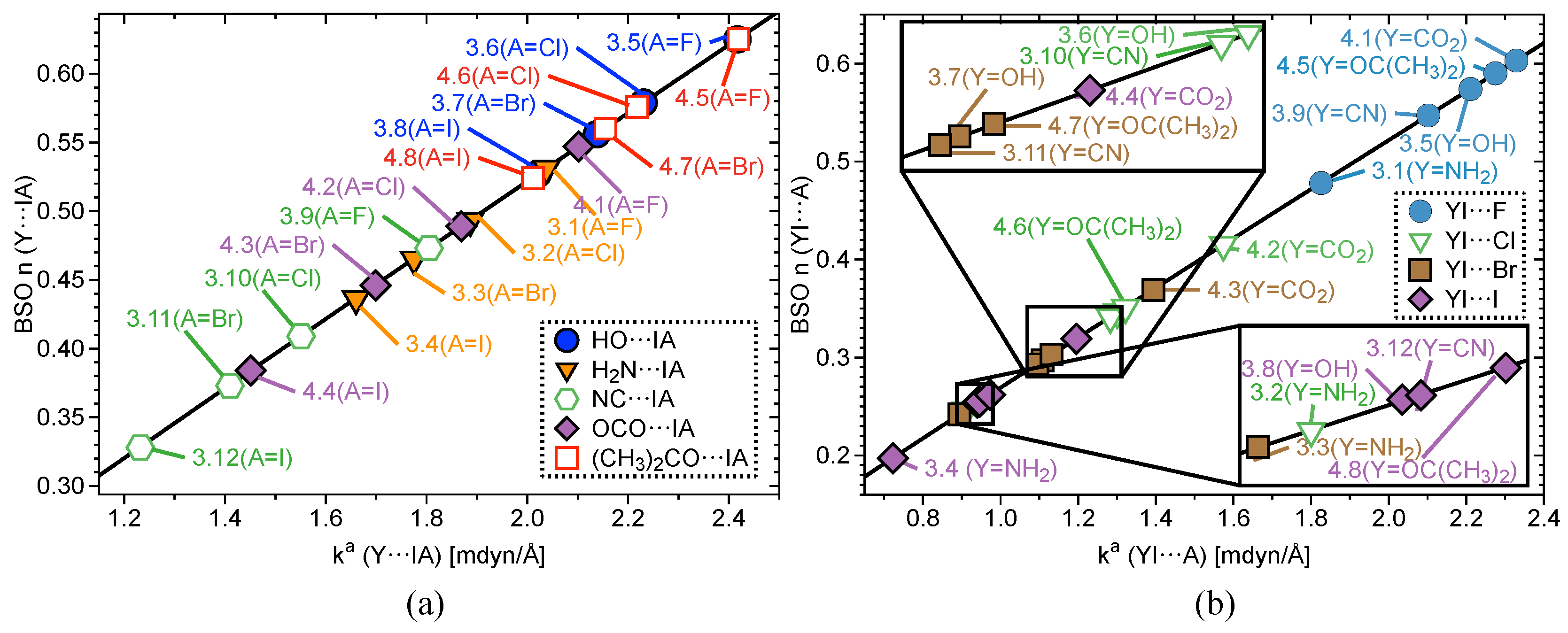
(a) BSO versus for of Y⋯IA (3.1–4.8) (b) and BSO versus of YI⋯A for complexes 3.1–4.8 according to eq 2, where A = the axial halogen atom and Y = the non-halogen atom bound axial to I.
Figure 3.
(a) BSO versus for of Y⋯IA (3.1–4.8) (b) and BSO versus of YI⋯A for complexes 3.1–4.8 according to eq 2, where A = the axial halogen atom and Y = the non-halogen atom bound axial to I.

Figure 4.
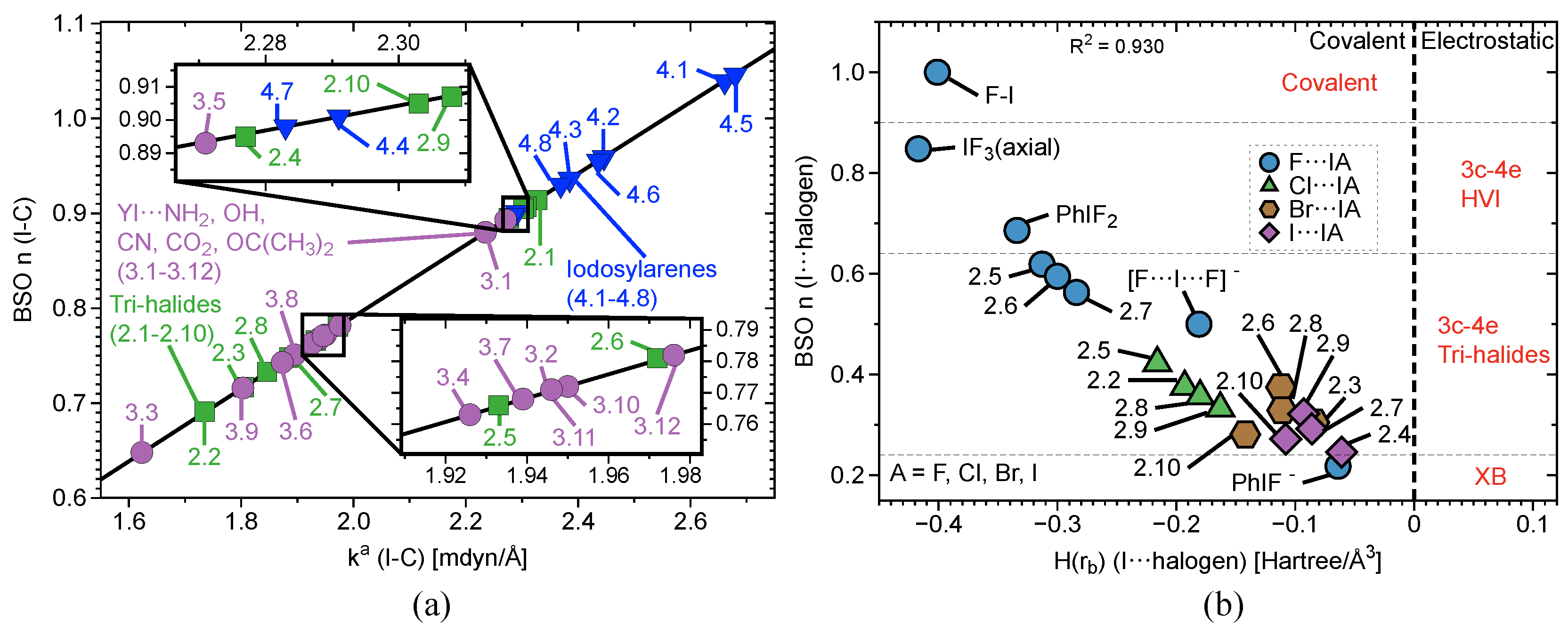
(a) BSO versus () of I–Ph (2.1–3.12) and I-benzene (Group 4) according to eq 2. BSO for the equatorial I–C bonds has been scaled by a factor of 1.517. (b) Comparison of BSO with of all halogen–iodine interactions in complexes 1.1–2.10. The vertical dashed line separates the electrostatic region from the covalent region.
Figure 4.
(a) BSO versus () of I–Ph (2.1–3.12) and I-benzene (Group 4) according to eq 2. BSO for the equatorial I–C bonds has been scaled by a factor of 1.517. (b) Comparison of BSO with of all halogen–iodine interactions in complexes 1.1–2.10. The vertical dashed line separates the electrostatic region from the covalent region.

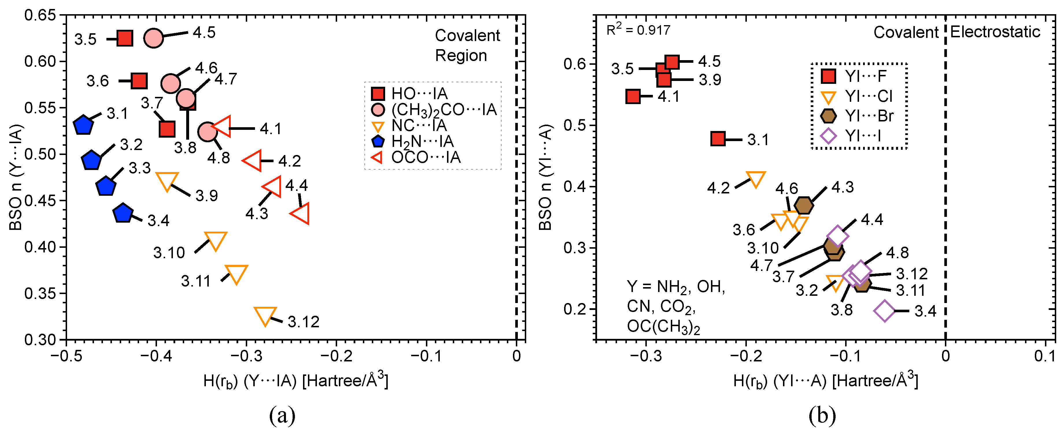
Figure 5.
(a) Comparison of BSO with of iodine-non halogen axial atom (Y⋯IA) interactions in complexes 3.1–4.8 and (b) a comparison of BSO with of axial halogen-iodine (YI⋯A) interactions in complexes 3.1–4.8. The vertical dashed line separates the electrostatic region from the covalent region.
Figure 5.
(a) Comparison of BSO with of iodine-non halogen axial atom (Y⋯IA) interactions in complexes 3.1–4.8 and (b) a comparison of BSO with of axial halogen-iodine (YI⋯A) interactions in complexes 3.1–4.8. The vertical dashed line separates the electrostatic region from the covalent region.

Table 1.
Bond distance (r), , , BSO , , , and %3c–4e for Y–I (1.1), Y–I⋯A (1.3), and Y⋯I⋯A bonds in 1.2, 1.4–4.8, where Y = A in 2.1–2.4, Y–I = the stronger of the two axial bonds in 1.3 and 2.5–4.8.
Table 1.
Bond distance (r), , , BSO , , , and %3c–4e for Y–I (1.1), Y–I⋯A (1.3), and Y⋯I⋯A bonds in 1.2, 1.4–4.8, where Y = A in 2.1–2.4, Y–I = the stronger of the two axial bonds in 1.3 and 2.5–4.8.
| # | Bond Analyzed | r | BSO n | r | BSO n | %3c–4e | |||||||||
|---|---|---|---|---|---|---|---|---|---|---|---|---|---|---|---|
| (Y–I; I–A) | (Y–I) | (Y–I) | (Y–I) | (Y–I) | (Y–I) | (Y–I) | (I–A) | (I–A) | (I–A) | (I–A) | (I–A) | (I–A) | |||
| Group1 | 1.1 | F–I | 1.921 | 3.953 | 1.000 | 637 | 0.900 | −0.401 | - | - | - | - | - | - | - |
| 1.2 | F–I; I–F | 2.089 | 1.913 | 0.500 | 443 | 0.615 | −0.181 | 2.089 | 1.913 | 0.500 | 443 | 0.615 | −0.181 | 100 | |
| 1.3 | C–I; I–F | 2.173 | 1.843 | 0.482 | 534 | 0.761 | −0.359 | 2.282 | 0.803 | 0.218 | 287 | 0.428 | −0.064 | 45 | |
| 1.4 | F–I; I–F | 1.951 | 3.327 | 0.848 | 585 | 0.875 | −0.417 | 1.951 | 3.327 | 0.848 | 585 | 0.875 | −0.417 | 100 | |
Group2 | 2.1 | F–I; I F | 1.997 | 2.666 | 0.686 | 523 | 0.783 | −0.334 | 1.997 | 2.666 | 0.686 | 523 | 0.783 | −0.334 | 100 |
| 2.2 | Cl–I; I–Cl | 2.481 | 1.420 | 0.376 | 297 | 0.542 | −0.193 | 2.481 | 1.420 | 0.376 | 297 | 0.542 | −0.193 | 100 | |
| 2.3 | Br–I; I–Br | 2.651 | 1.140 | 0.305 | 155 | 0.465 | −0.136 | 2.651 | 1.140 | 0.305 | 155 | 0.465 | −0.136 | 100 | |
| 2.4 | I–I; I–I | 2.892 | 0.910 | 0.246 | 199 | 0.380 | −0.092 | 2.892 | 0.904 | 0.244 | 156 | 0.380 | −0.092 | 100 | |
| 2.5 | F–I; I–Cl | 2.014 | 2.395 | 0.619 | 496 | 0.759 | −0.313 | 2.454 | 1.606 | 0.423 | 315 | 0.567 | −0.216 | 68 | |
| 2.6 | F–I; I–Br | 2.025 | 2.296 | 0.595 | 486 | 0.745 | −0.300 | 2.606 | 1.416 | 0.375 | 222 | 0.503 | −0.164 | 63 | |
| 2.7 | F–I; I–I) | 2.039 | 2.168 | 0.563 | 472 | 0.725 | −0.284 | 2.821 | 1.208 | 0.322 | 180 | 0.431 | −0.123 | 57 | |
| 2.8 | Cl–I; I–Br | 2.498 | 1.344 | 0.357 | 288 | 0.525 | −0.180 | 2.632 | 1.235 | 0.329 | 208 | 0.481 | −0.147 | 92 | |
| 2.9 | Cl–I; I–I | 2.522 | 1.250 | 0.333 | 278 | 0.503 | −0.163 | 2.847 | 1.088 | 0.292 | 171 | 0.412 | −0.111 | 88 | |
| 2.10 | Br–I; I–I | 2.677 | 1.045 | 0.281 | 191 | 0.443 | −0.121 | 2.865 | 1.011 | 0.272 | 164 | 0.399 | −0.103 | 97 | |
Group 3 | 3.1 | N–I; I–F | 2.080 | 2.038 | 0.531 | 524 | 0.854 | −0.481 | 2.084 | 1.826 | 0.478 | 433 | 0.654 | −0.228 | 90 |
| 3.2 | N–I; I–Cl | 2.087 | 1.887 | 0.493 | 504 | 0.851 | −0.472 | 2.611 | 0.911 | 0.246 | 238 | 0.419 | −0.110 | 50 | |
| 3.3 | N–I; I–Br | 2.100 | 1.775 | 0.465 | 489 | 0.835 | −0.456 | 2.767 | 0.894 | 0.242 | 177 | 0.371 | −0.084 | 52 | |
| 3.4 | N–I; I–I | 2.113 | 1.660 | 0.436 | 473 | 0.817 | −0.437 | 2.998 | 0.723 | 0.197 | 139 | 0.315 | −0.061 | 45 | |
| 3.5 | O–I; I–F | 2.031 | 2.417 | 0.625 | 537 | 0.836 | −0.435 | 2.036 | 2.275 | 0.590 | 483 | 0.722 | −0.283 | 94 | |
| 3.6 | O–I; I–Cl | 2.042 | 2.231 | 0.579 | 516 | 0.822 | −0.419 | 2.520 | 1.301 | 0.346 | 284 | 0.500 | −0.165 | 60 | |
| 3.7 | O–I; I–Br | 2.051 | 2.138 | 0.556 | 505 | 0.761 | −0.365 | 2.676 | 1.108 | 0.297 | 197 | 0.425 | −0.112 | 53 | |
| 3.8 | O–I; I–I | 2.064 | 2.021 | 0.527 | 491 | 0.790 | −0.388 | 2.895 | 0.940 | 0.254 | 159 | 0.378 | −0.093 | 48 | |
| 3.9 | F–I; I–C | 2.038 | 2.211 | 0.574 | 476 | 0.722 | −0.282 | 2.154 | 1.805 | 0.473 | 529 | 0.763 | −0.388 | 82 | |
| 3.10 | C–I; I–Cl | 2.174 | 1.551 | 0.409 | 490 | 0.705 | −0.334 | 2.519 | 1.283 | 0.341 | 282 | 0.474 | −0.147 | 83 | |
| 3.11 | C–I; I–Br | 2.189 | 1.410 | 0.373 | 467 | 0.681 | −0.311 | 2.672 | 1.095 | 0.293 | 195 | 0.421 | −0.111 | 79 | |
| 3.12 | C–I; I–I | 2.213 | 1.232 | 0.328 | 437 | 0.644 | −0.279 | 2.887 | 0.946 | 0.255 | 159 | 0.365 | −0.086 | 78 | |
Group 4 | 4.1 | F–I; I–O | 1.993 | 2.622 | 0.675 | 519 | 0.757 | −0.313 | 2.079 | 2.102 | 0.547 | 501 | 0.719 | −0.325 | 81 |
| 4.2 | O–I; I–Cl | 2.102 | 1.869 | 0.489 | 473 | 0.682 | −0.291 | 2.448 | 1.574 | 0.415 | 312 | 0.536 | −0.190 | 85 | |
| 4.3 | O–I; I–Br | 2.117 | 1.699 | 0.446 | 451 | 0.657 | −0.269 | 2.598 | 1.394 | 0.369 | 221 | 0.473 | −0.142 | 83 | |
| 4.4 | O–I; I–I | 2.141 | 1.451 | 0.384 | 416 | 0.623 | −0.238 | 2.809 | 1.195 | 0.319 | 179 | 0.408 | −0.108 | 83 | |
| 4.5 | O–I; I–F | 2.032 | 2.419 | 0.625 | 538 | 0.800 | −0.403 | 2.024 | 2.329 | 0.603 | 489 | 0.710 | −0.274 | 96 | |
| 4.6 | O–I; I–Cl | 2.041 | 2.218 | 0.576 | 515 | 0.781 | −0.384 | 2.503 | 1.322 | 0.351 | 286 | 0.482 | −0.153 | 61 | |
| 4.7 | O–I; I–Br | 2.050 | 2.155 | 0.560 | 507 | 0.763 | −0.367 | 2.658 | 1.131 | 0.303 | 199 | 0.424 | −0.113 | 54 | |
| 4.8 | O–I; I–I | 2.063 | 2.011 | 0.524 | 490 | 0.739 | −0.343 | 2.875 | 0.973 | 0.262 | 161 | 0.364 | −0.085 | 50 |
a Calculated at the B97X-D/aug-cc-pVTZ level of theory. r are given in Å, in e/Å, in Hartree/Å, in mdyn/Å, BSO , %3c–4e calculated in terms of BSO n, and in cm. In Group 4, R = CO (4.1–4.4). For 4.5–4.8, R = C(CH).
Table 2.
r, , , and local vibrational data for I-equatorial ligand (I–F, I–C) interactions of complexes 1.4–4.8, where BSO is scaled by a factor of 1.517.
Table 2.
r, , , and local vibrational data for I-equatorial ligand (I–F, I–C) interactions of complexes 1.4–4.8, where BSO is scaled by a factor of 1.517.
| # | Bond Analyzed | r | BSO n (Scaled) | |||||
|---|---|---|---|---|---|---|---|---|
| Group 1 | 1.4 | I–F | 1.876 | 1.037 | −0.569 | 4.087 | 1.565 | 648 |
Group 2 | 2.1 | I–C | 2.123 | 0.895 | −0.476 | 2.327 | 0.914 | 600 |
| 2.2 | I–C | 2.116 | 0.895 | −0.476 | 1.735 | 0.691 | 518 | |
| 2.3 | I–C | 2.107 | 0.905 | −0.488 | 2.277 | 0.717 | 594 | |
| 2.4 | I–C | 2.107 | 0.901 | −0.484 | 1.805 | 0.895 | 529 | |
| 2.5 | I–C | 2.129 | 0.880 | −0.461 | 1.933 | 0.766 | 547 | |
| 2.6 | I–C | 2.125 | 0.884 | −0.466 | 1.972 | 0.781 | 553 | |
| 2.7 | I–C | 2.120 | 0.891 | −0.473 | 1.886 | 0.748 | 540 | |
| 2.8 | I–C | 2.112 | 0.900 | −0.482 | 1.846 | 0.733 | 535 | |
| 2.9 | I–C | 2.103 | 0.912 | −0.495 | 2.308 | 0.907 | 598 | |
| 2.10 | I–C | 2.105 | 0.907 | −0.490 | 2.303 | 0.905 | 597 | |
Group 3 | 3.1 | I–C | 2.139 | 0.869 | −0.452 | 2.235 | 0.880 | 588 |
| 3.2 | I–C | 2.157 | 0.836 | −0.418 | 1.950 | 0.772 | 549 | |
| 3.3 | I–C | 2.142 | 0.858 | −0.44 0 | 1.623 | 0.648 | 501 | |
| 3.4 | I–C | 2.132 | 0.872 | −0.455 | 1.926 | 0.763 | 546 | |
| 3.5 | I–C | 2.128 | 0.888 | −0.471 | 2.271 | 0.893 | 593 | |
| 3.6 | I–C | 2.133 | 0.874 | −0.457 | 1.895 | 0.751 | 542 | |
| 3.7 | I–C | 2.130 | 0.834 | −0.424 | 1.939 | 0.768 | 548 | |
| 3.8 | I–C | 2.125 | 0.885 | −0.468 | 1.873 | 0.743 | 538 | |
| 3.9 | I–C | 2.138 | 0.865 | −0.445 | 1.803 | 0.716 | 528 | |
| 3.10 | I–C | 2.130 | 0.822 | −0.402 | 1.926 | 0.763 | 546 | |
| 3.11 | I–C | 2.127 | 0.829 | −0.409 | 1.946 | 0.771 | 549 | |
| 3.12 | I–C | 2.123 | 0.841 | −0.421 | 1.976 | 0.782 | 553 | |
Group 4 | 4.1 | I–C | 2.090 | 0.907 | −0.490 | 2.661 | 1.039 | 642 |
| 4.2 | I–C | 2.110 | 0.863 | −0.445 | 2.446 | 0.959 | 615 | |
| 4.3 | I–C | 2.115 | 0.852 | −0.434 | 2.385 | 0.936 | 608 | |
| 4.4 | I–C | 2.123 | 0.838 | −0.421 | 2.291 | 0.901 | 596 | |
| 4.5 | I–C | 2.094 | 0.901 | −0.485 | 2.680 | 1.046 | 644 | |
| 4.6 | I–C | 2.113 | 0.860 | −0.444 | 2.436 | 0.955 | 614 | |
| 4.7 | I–C | 2.118 | 0.851 | −0.434 | 2.369 | 0.930 | 606 | |
| 4.8 | I–C | 2.124 | 0.838 | −0.422 | 2.283 | 0.898 | 594 |
a Calculated at the B97X-D/aug-cc-pVTZ level of theory. r are given in Å, in e/Å, in Hartree/Å, in mdyn/Å, BSO , and in cm. In Group 4, R = CO (4.1–4.4). For 4.5–4.8, R = C(CH).
© 2019 by the authors. Licensee MDPI, Basel, Switzerland. This article is an open access article distributed under the terms and conditions of the Creative Commons Attribution (CC BY) license (http://creativecommons.org/licenses/by/4.0/).
Share and Cite
MDPI and ACS Style
Yannacone, S.; Oliveira, V.; Verma, N.; Kraka, E. A Continuum from Halogen Bonds to Covalent Bonds: Where Do λ3 Iodanes Fit? Inorganics 2019, 7, 47. https://0-doi-org.brum.beds.ac.uk/10.3390/inorganics7040047
AMA Style
Yannacone S, Oliveira V, Verma N, Kraka E. A Continuum from Halogen Bonds to Covalent Bonds: Where Do λ3 Iodanes Fit? Inorganics. 2019; 7(4):47. https://0-doi-org.brum.beds.ac.uk/10.3390/inorganics7040047
Chicago/Turabian StyleYannacone, Seth, Vytor Oliveira, Niraj Verma, and Elfi Kraka. 2019. "A Continuum from Halogen Bonds to Covalent Bonds: Where Do λ3 Iodanes Fit?" Inorganics 7, no. 4: 47. https://0-doi-org.brum.beds.ac.uk/10.3390/inorganics7040047
Note that from the first issue of 2016, this journal uses article numbers instead of page numbers. See further details here.