Ant Colony Optimization for Multiple Pickup and Multiple Delivery Vehicle Routing Problem with Time Window and Heterogeneous Fleets

Abstract

This study focuses on solving the vehicle routing problem (VRP) of E-logistics service providers. In our problem, each vehicle must visit some pick up nodes first, for instance, warehouses to pick up the orders then makes deliveries for customers in the list. Each pickup node has its own list of more than one customers requiring delivery. The objective is to minimize the total travelling cost while real-world application constraints, such as heterogeneous vehicles, capacity limits, time window, driver working duration, etc. are still considered. This research firstly proposes a mathematical model for this multiple pickup and multiple delivery vehicle routing problem with time window and heterogeneous fleets (MPMDVRPTWHF). In the next step, the ant colony optimization algorithm is studied to solve the problem in the large-scale.

1. Introduction

Supply chain management, which is the key part of any organization, has a huge impact on the quality of service to customers. It is a chain consisting of components from the supply sources to the end customers. In the chain, transportation plays the decision function in providing the right product to the right customer at the right time which is responsible for moving products from suppliers to end customers. To satisfy the continuous changes in customer requirements in terms of the quality of delivery time and the competitive price, the organization must build a responsive supply chain network to serve edges of customer demand and offer the acceptable service fee toward customers.

According to the estimates method of logistics costs in the United Stated proposed by The Economic and Social Commission for Asia and the Pacific (ESCAP) https://www.unescap.org/sites/default/d8files/pub_2194_Appendix.pdf (accessed on 21 April 2021), transportation costs in logistics cost accounts for more than 60% of the total cost in which transportation costs include costs for transporting finished goods from plants and vendors through distribution centers to final customers, and it includes costs for all modes such as trucking, rail transport, water and oil pipeline; and both domestics and international transport and related custom clearance cost. Therefore, cost optimization in transportation is extremely necessary for providing the best price—offer service and competing with others while fitting some practical requirements such as a variety of time window demanded from each customer, stochastic demand, various types of fleet, and some unpredicted events, etc. Therefore, the last-mile delivery service and E—commerce logistics have been emerged and grown extremely rapidly in the logistics industry.

This study is inspired by the real case of truck routing optimization in a delivery company which has a dense warehouses network. The problem objective is to output a set of routes from the nodes set with the aim to minimize the total travelling distance and cost consumption. The model design is required that vehicles starting from a depot and moving through warehouses for both or in turn picking up and delivering goods. More particularly, it is a mixed linehaul and backhaul VRP which might be only demand of picking or delivering or both in each node, and the serving order of pickup or delivery in each one is arbitrary depending on the time constraints and optimality of objective function. In addition, some practical constraints such as time window, heterogenous fleets of vehicle, capacity limit, and working duration of drivers are also considered for the case. The multiple pickup and multiple delivery vehicle routing problem with time window and heterogeneous fleets (MPMDVRPTWHF) method is employed to solve the case.

The Vehicle Routing Problem with Time window (VRPTW) concerns the problem of minimizing costs when a fleet of vehicles has to deliver goods from the depot to a set of customers while not violating a set of required constraints [1]. The problem proposed in this paper can be called a variant of VRPTW which can solve the logistics network pattern that has a set of pickup points that have goods loaded and a set of delivery points that have goods delivered while satisfying the constraint of time-window, a heterogeneous fleet of vehicles and route length limit. The mathematical model and applied algorithm proposed by this paper can help to solve the problem patterns such as retail network, e-logistics network, distribution network, reversed network, etc., which have the same characteristics in the network, having goods that need to be picked up at several factories or warehouses and distributed to a set of customers or retailers.

The VRP was first introduced by [2] in the truck dispatching problem. In their study, they proposed the first mathematical programming formulation and algorithmic approach to the delivery of gasoline to the gas station. A few years later, Ref. [3] introduced an effective greedy heuristic improving Dantzig-Ramser approach. From the basics of the two mentioned paper, many exact and approximate approaches were proposed to find the nearest or exact solution of the diverse versions of the VRP. Researched by [4], there are several versions of VRPs with different problem assumptions and objective concentrations. The first basic of the problem is the Capacitated VRP (CVRP). The CVRP is illustrated in [3], where the vehicles are homogeneous and based on a single departure depot. All the customers are delivery points, the demand is constant and may not be split. The main restriction in the problem is vehicle capacity. Furthermore, to be used in a real-life application, researchers also study the model of multiple depot vehicle routing problem with time window under shared depot resources [5]. The VRPTW is an adjusted version of CVRP in which the capacity constraint is still in consideration and each customer is associated with a serving time requirement $\left[a_i{b}_i\right]$, called a time window [6,7]. In a time instant, the travelling time $t_{ij}$ of the arc $(i,j)$, the service time $s_i$ are given. In case of early arrival at customer location, it can wait until the time instant $a_i$. It is assumed that vehicles leave the depot at time instant 0 to support the time window defining. Another extension of CVRP is The VRP with Backhauls (VRPB). In the problem, there are two subsets of customers. The first subset contains linehaul customers requiring a given quantity of products to be delivered and the second subset contains m backhaul customers from which the given required pickup quantity need. The route assigned to serve both types of customers must serve all the linehaul customers before the backhaul customers.

Another version of the typical VRP is VRP with Pickup and Delivery (VRPPPD). Each customer is associated with the delivery quantity $d_i$ and the pickup quantity $p_i$, and $O_i$ is the origin pickup point of the delivery quantity; $D_i$ is the destination point of goods picked up at the customer. A variety of practical situations can be modeled as pickup and delivery problem which can be listed such as school bus routing and scheduling, reversed logistics and dispatching network in E-logistics. The VRPPPD can be illustrated in several research proposed by [8] in which the pickup and delivery problem with time windows (PDPTW) is studied and an exact method is proposed to solve the problem; Ref. [9] in which they proposed a formulation for pickup and delivery problem with time window developing a novel modeling strategy assigning vehicles to routes explicitly in two-index flow formulation.

Since the VRPTW is an NP-hard problem, it can solve the small-sized problem effectively in term of time using exact solution methods introduced by [1,10,11,12,13]. Besides, heuristics is introduced to help solve large-sized problems more optimally in computational time. Following [14], the exact algorithm can be divided into three categories: direct tree search methods, dynamic programming, and integer linear programming. As the number of proposed exact algorithms is very large, the research proposed by [15] adopted a column generation algorithm for vehicle scheduling and routing problems, Ref. [16] proposes minimum K-trees algorithm to find optimal solution of vehicle routing problem, Ref. [17] adopts a branch-and-cut-and-price algorithm for solving a pickup-and-delivery problem with time window, while [8] devises an exact algorithm based on a set portioning integer formulation with a bounding procedure. A detailed review of exact and approximate algorithms can be found in [14]. Several other studies investigate and use heuristics and metaheuristic algorithms to solve vehicle routing problem. Some state-of-the-art metaheuristics approach can be listed in detail such as simulated annealing algorithm, genetic algorithm, ant colony optimization algorithm, firefly algorithm, etc. in [18] which reviews several metaheuristics and make comparison of them.

Generally, an exact method intends to give the exact optimal solution; however, it is suitable for small-size problems. On the other hand, the heuristics or meta-heuristics output the near-optimal solution, and it can deal with the large-size problem mentioned in [19] which is advantageous in term of computational time and the solution quality. There are some heuristics strategies introduced to solve well-known VRP such as the space-filling curve with optimal partitioning heuristics [20], three-phase heuristics [21] developed by combining a heuristic-based clustering algorithm solving VRP. A summary and literature review of several important and state-of-art modern heuristics can be found in the study by [22,23].

In this paper, ant colony optimization (ACO) approach is proposed to solve Multiple pickup and multiple delivery vehicle routing problem with time window and heterogeneous fleets. The ACO algorithm was first introduced by [24]. It is built based on the ant behavior in real life to find food with the optimal path from their nest to food sources. Pheromones substances released by ants on the trails is a form of communication among the ants and help them travel to the food optimally. Reviewed from the previous study on this algorithm, there is a plenty of variants and studies applying ACO. The ant system first was developed by [25]. Since then, many researchers have studied and published new methods to improve the original ACO by applying other algorithms into the ACO to tackle the larger-sized CVRP [26]. For instance, a hybrid approach proposed by [27] combining AS with the savings algorithm to solve the CVRP, improved ACO for the, multiple-depot vehicle routing problem with time windows [28] and also there are some other researchers contributing to improve ACO method such as [29] with a new hybrid ant colony optimization algorithm [30,31].

The rest of the paper is organized as follows. The next section presents the mathematical model for MPMDVRPTWHF while the third section describes the framework for applying ACO to solve the large scale problem. Finally, the computational result and conclusions are presented in the final section.

2. Mathematical Model

Inspired by the study on a VRPTW case study of fresh food distribution center [32], service nodes are divided into two subsets: pickup set P and delivery set D where $\left|P\right|=n$ and $\left|D\right|=m$. The starting depot is node 0. The ending depot is node $(n+m+1)$. If one node requires both delivery and pickup, that node will be replicated. Each vehicle in the fleet has its own operation cost and capacity. The set R contains pairs of $(i,j)$ if the order exists between pickup node i and delivery node j.

Equation (1) represents the objective function which aims to minimize the total cost of traveling

$$min\sum _{k\in K}\sum _{i,j\in C}{x}_{ij}^k{d}_{ij}{\gamma }_k$$

(1)

The Equation (2) ensure that each node must be served at least by one vehicle

$$\sum _{k\in K}\sum _{j\in C_1}{x}_{ij}^k\ge 1\forall i\in C\backslash \{0,n+m+1\}$$

(2)

If there is an order between pickup node i and delivery node j, this order must be served by the same vehilce k. This constraint is shown in Equation (3)

$$\sum _{h\in C_2}{x}_{hi}^k-\sum _{m\in C_2}{x}_{mj}^k=0\forall k\in K,\forall (i,j)\in R$$

(3)

Equations (4) and (5) claim that if an vehicle is used, its route must go through starting depot and ending depot at least once.

$$\sum _{j\in C_1}{x}_{0j}^k\le 1,\forall k\in K$$

(4)

$$\sum _{j\in C_2}{x}_{j,n+m+1}^k\le 1,\forall k\in K$$

(5)

Equation (6) says that if a vehicle visit a node, then it also has to leave that node

$$\sum _{i\in C_2}{x}_{ij}^k=\sum _{h\in C_1}{x}_{jh}^k\forall j\in C\backslash \{0,n+m+1\},h\ne i,j\ne i,k\in K.$$

(6)

Subtour elimination, time constraint and load constraints are integrated in Equation (7) and (8).

$$T_j^k\ge T_i^k+(t_{ij}+s_i)-BigM(1-x_{ij}^k),\forall k\in K,i\in C_2,j\in C_1$$

(7)

$$L_j^k\ge L_i^k+q_j-BigM(1-x_{ij}^k),\forall k\in K,i\in C_2,j\in C_1,k\in K,i\ne j$$

(8)

The pickup node must be visited before the delivery node in case there is an order between them is expressed by Equation (9)

$$T_i^k+R_{ij}(t_{ij}+s_i)\le T_j^k,\forall k\in K,i\in P,j\in D$$

(9)

Time window constraint is shown in Equation (10)

$$e_i\le T_i^k\le l_i,\forall i\in C\backslash \{0,n+m+1\}k\in K$$

(10)

The capacity bound constraint is presented in Equation (11)

$$max(0,q_i)\le L_i^k\le min(Q_k,Q_k+q_i),\forall i\in C,k\in K$$

(11)

The maximum working duration is shown in Equation (12) while Equation (13) limits the number of vehicles can be used

$$T_{n+m+1}^k-T_0^k\le t_{max},\forall k\in K$$

(12)

$$\sum _{k\in K}\sum _{j\in C}{x}_{0j}^k\le M$$

(13)

This model is used to solve the problem in the small and average scale to create the benchmark for ACO.

3. Solution Approach

Ant Colony Optimization (ACO) algorithm was adopted to solve the proposed problem. It is a probabilistic optimization that simulates the social behavior of ant colonies, a kind of species that can find the shortest route from the nest to the food source and back. They choose the path based on a chemical substance called pheromone secreted from the ants to go through previously. The repetition of the above mechanism represents the auto-catalytic behavior of a real ant colony where the more the ant follow a trail, the more attractiveness the trail become.

The algorithm we propose for the MPMDVRPTWHF has been developed to fit featured constraints in the studied problem including using heterogeneous fleet of vehicles, considering time window, those two constraints can be considered as challenging points for the majority of methods known from the literature. Additionally, the model can be applied to the system in which it has multiple pickup points, and each pickup point has multiple delivery destination, therefore, it is not the same as some previous studies whose system have a monopoly pickup source and delivery to several destination, the relationship between pickup node set and delivery node set must be considered when choosing the next node to visit following the rule that pickup node must be choose before their delivery node set. Moreover, we have set up in the algorithm operation that the ant will check each next chosen node if it satisfies the set of constraints or not simultaneously when the next node is chosen. Therefore, the solution proposed by the ant will fit exactly with the scheme constraints.

The main tasks considered in this ACO algorithm are initialization of necessary parameters, solution construction by ants and pheromones substance management. Overall, the main procedures of the proposed algorithm are illustrated in the flowchart of Figure 1.

3.1. Initialization of the Parameter

Following the research proposed by [28], all the related parameters are setup as follows: $m=22$ ants, $\alpha =2$, $\beta =5$, $\rho =0.80$, $\theta =80$, $\sigma =3$ elitist ants.

Each arc $(i,j)$ of the graph $G=(N,A)$ is associated with a variable ${\tau }_{ij}$ called pheromone trail. The pheromone intensity on an arc indicates the level of probabilities that the following direction gives the better solution. Therefore, at each node, the ant will decide the next node to visit based on the level of pheromone on trails. The higher level of pheromone, the higher probability the trail would be chosen. Initially, a constant amount of pheromone is allocated to all the arcs. The probability of the kth ant at node choosing to move to node j using the pheromone trail ${\tau }_{ij}$ is given by:

$$p_{ij}^k=\frac{{\left[{\tau }_{ij}\right]}^{\alpha }{\left[{\eta }_{ij}\right]}^{\beta }}{{\sum }_{l\in N_j^k}{\left[{\tau }_{ij}\right]}^{\alpha }{\left[{\eta }_{ij}\right]}^{\beta }},\mathrm{if}j\in N_i^k$$

(14)

$\eta =1/d_{ij}$ is a heuristic value. ${\tau }_{ij}$ denotes the pheromone concentration on the edge traversed from node i to node j. The parameters $\alpha$, $\beta$ are the relative influence of pheromone concentration and the heuristic value. Specifically, ${\tau }_{ij}$ indicates how good the choice of the next node from the current one, ${\eta }_{ij}$ implies the promising of the choice of the next node j from the current node i. The set of probabilities will be equal to 1 initially.

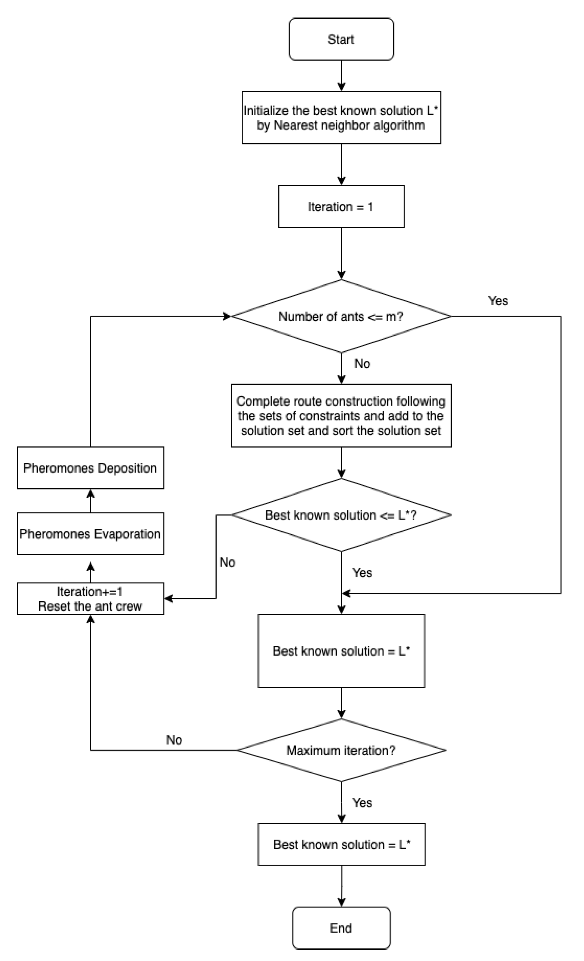
3.2. Solution Construction

In the ACO, each artificial ant will generate the solution by taking vehicles from the vehicle set starting from the depot to construct the next node which satisfies the set of constraints. The routes will be built by the ant until the capacity or the limit of route length is met, or the time window constraint is violated. Specifically, the next node constructed by the ant will go through a constraint checking process and if it is successfully added to the route, all the related variables will be updated to be used for the next node drawing. The route set by all the ant crew will be recorded in a solution set which would be used for obtaining the best solution from each iteration and update the current best-known solution $L^{*}$. The pseudocode of the complete ACO algorithm is illustrated as below.

The process of using pheromones to determine the promising optimal route involves the pheromone update which consists of pheromone deposition and pheromone evaporation. A pheromone trails update would be conducted after all the artificial ants have improved the solutions. In addition, this factor is also the main feature of ACO algorithm, determining the ants’ performance and the quality of solution found. In the proposed ACO algorithm, pheromone modifications would employ the usual pheromone evaporation while the pheromone deposition would be referred to [33]. In pheromone evaporation, the pheromone concentration on all trails could be decreased by a constant factor which is given by following equation:

$${\tau }_{ij}=\left(\rho +\frac{\theta }{L^{avg}}\right){\tau }_{ij}\forall (i,j)\in A$$

(15)

where $0\le \left(\rho +\frac{\theta }{L^{avg}}\right)\le 1$ is an evaporation factor, $0\le \rho \le 1$ is the trail persistence, $\theta$ is a constant. $L^{avg}={\sum }_{k=1}^m\frac{L^k}{m}$ is the average total distance found by m artificial ants per iteration and $L^k$ is the total distance obtained by the solution of an artificial ant k. The idea of the pheromone evaporation is to simulate the evaporation process in nature which depends on the length of path travelled by an ant.

After the evaporation process, only the best and the elitist ants can update the pheromone by depositing the substance to the path they travelled following the equation below:

$${\tau }_{ij}={\tau }_{ij}+\sum _{\lambda =1}^{\sigma -1}\Delta {\tau }_{ij}^{\lambda }+\Delta {\tau }_{ij}^{*}$$

(16)

where

$$\Delta {\tau }_{ij}^{\lambda }=\left\{\begin{array}{cc}\frac{\sigma -\lambda }{L^{\lambda }},\hfill & \mathrm{if}\mathrm{the}\lambda \mathrm{th}\mathrm{best}\mathrm{ant}\mathrm{travels}\mathrm{on}\mathrm{edge}(i,j)\hfill \\ 0\hfill & otherwise\hfill \end{array}\right.$$

(17)

$$\Delta {\tau }_{ij}^{*}=\left\{\begin{array}{cc}\frac{\sigma }{L^{*}},\hfill & \mathrm{if}\mathrm{edge}(i,j)\mathrm{is}\mathrm{part}\mathrm{of}\mathrm{the}\mathrm{best}\mathrm{solution}\hfill \\ 0\hfill & otherwise\hfill \end{array}\right.$$

(18)

Following is the description of ant colony algorithm for multiple pickup and multiple delivery vehicle routing problem with time window and heterogeneous fleets (ACO for the MPMDVRPTWHF) (Algorithm 1).

Algorithm 1: ACO for the MPMDVRPTWHF

There are two types of pheromone deposition laid down the trails during the pheromone update process with Equations (17) and (18) above. First, the best-so-far solution (objective value $L^{*}$) found at the start of the ACO algorithm will be update if $\sigma$ elitist ants had traversed it. That update of pheromone by the elitist ants is called $\Delta {\tau }_{ij}^{*}$. Second, only the $(\sigma -1)$ best ants out of m ants of the current iteration can lay the pheromone on the trails they have traversed. The amount of pheromone laid down by the ants which equals to $\Delta {\tau }_{ij}^{\lambda }$ is determined by their rank $\lambda$ and their solution quality $L^{\lambda }$. In brief, the idea to establish the elitist ants to emphasize the reinforcement of the edges belonging to the best-so-far solution after running the iteration and it would be the guidance for the succeeding iterations. On the contrary, the idea of ranking the ants by $\lambda$ is suggested in [20] and aims to minimize the emphasis of pheromone laid by many ants caused by suboptimal routes. Figure 2 shows example of constructing solution by the ACO algorithm.

4. Computational Results and Conclusion

This section is devoted to the experimental evaluation of ACO algorithm on some standard benchmark instances. The benchmark adopted in the experimental design will be described in detail in Section 4.1 while in Section 4.2 the results achieved by the ACO algorithm will be presented and compared with those of exact method proposed by CPLEX solver to validate our solution method. Finally, Section 4.3 will show that the proposed method can be applied in practical cases. To evaluate the validation of the solution, two methods would be tested by PYTHON and CPLEX software on Intel^® Core(TM) i5-8265U CPU @ 1.60 GHz 1.80 GHz.

4.1. Benchmark Description

The study adopts the instance set generated by Dominik Goeke (2017) used to solve Pickup and delivery problem with time windows and electric vehicles (PDPTW-EV), besides, it can also be used to validate the vehicle routing problem with time window (VRPTW) and Green vehicle routing problem (G-VRP). The generated benchmark instances have two sets: a set of 36 small-sized instances with 3–9 requests and an other set of 56 larger-sized instances with 50 requests. In this study, due to the limitation of CPLEX solver on solving large-scale problems, only the small-sized sets are considered to validate the proposed method solution. In addition, Section 4.3 will show the ability of the proposed method on solving large-scale problem. The instance set is shown in

Table 1. Result summaries of different instances.

Computational Result
Instance	ACO VRP			CPLEX	Gap
	Min	Max	Average
c101c6	1319.98	1319.98	1319.98	1319.98	0.00%
c103c6	1153.75	1153.75	1153.75	1153.75	0.00%
c206c6	1338.86	1338.86	1338.86	1338.86	0.00%
c208c6	902.69	902.69	902.69	902.69	0.00%
r104c6	1029.47	1029.47	1029.47	1029.47	0.00%
r105c6	831.31	831.31	831.31	831.31	0.00%
r202c6	885.63	885.63	885.63	885.63	0.00%
r203c6	1126.40	1126.40	1126.40	1126.40	0.00%
rc105c6	1465.66	1465.66	1465.66	1465.66	0.00%
rc108c6	1352.30	1352.30	1352.30	1352.30	0.00%
rc204c6	954.15	954.15	954.15	954.15	0.00%
rc208c6	925.42	925.42	925.42	925.42	0.00%
c104c10	2029.37	2029.37	2029.37	2029.37	0.00%
c205c10	1822.89	1822.89	1822.89	1822.89	0.00%
r201c10	1766.95	1766.95	1766.95	1766.95	0.00%
r203c10	1385.67	1385.67	1385.67	1385.67	0.00%
rc108c10	1916.49	1916.49	1916.49	1916.49	0.00%
rc201c10	2050.08	2050.08	2050.08	2050.08	0.00%
rc205c10	2463.76	2463.76	2463.76	2463.76	0.00%
c101c12	2167.13	2172.13	2169.33	2155.75	0.63%
c202c12	1851.35	1878.35	1858.75	1833.35	1.39%
r102c12	1518.96	1535.96	1525.16	1503.66	1.43%
r103c12	1227.01	1247.01	1240.81	1225.71	1.23%
rc102c12	2038.62	2162.62	2100.62	2035.12	3.22%
c103c16	2283.20	2502.33	2327.03	2283.20	1.92%
c106c16	1671.41	1701.41	1686.41	1631.41	3.37%
c202c16	2294.32	2375.74	2335.03	2283.22	2.27%
c208c16	2283.21	2433.93	2358.57	2283.21	3.30%
r105c16	2296.32	2336.32	2316.32	2247.45	3.06%
r202c16	3343.71	3443.71	3393.71	3311.95	2.47%
r209c16	2392.01	2408.79	2400.40	2332.01	2.93%
rc103c16	2794.23	2894.23	2844.23	2774.23	2.52%
rc108c16	2993.06	3093.06	3043.06	2970.06	2.46%
rc202c16	2912.30	3087.30	2999.80	2892.67	3.70%
rc204c16	3533.47	3663.25	3598.36	3519.47	2.24%
r102c18	2848.34	2884.23	2866.29	2765.34	3.65%
Avg.					1.16%

, and the instance sizes are also indicated in their names. The instances are available for download at http://www.vrp-rep.org/datasets/item/2019-0001.html (accessed on 21 April 2021).

There are some required modifications to the original instance set to be more appropriate to apply in the studied problem. Specifically, vehicle parameters, relation-set, and maximum working duration are added to the instance. The parameters of each vehicle includes its identifications, corresponding capacity and unit cost. This type of data will serve the constraint of heterogeneous truck fleets. The relation set represents the relationship between pickup points and their requesters while the maximum working durations limit the working time of drivers which serve the working duration constraint.

4.2. Comparison with Exact Solution

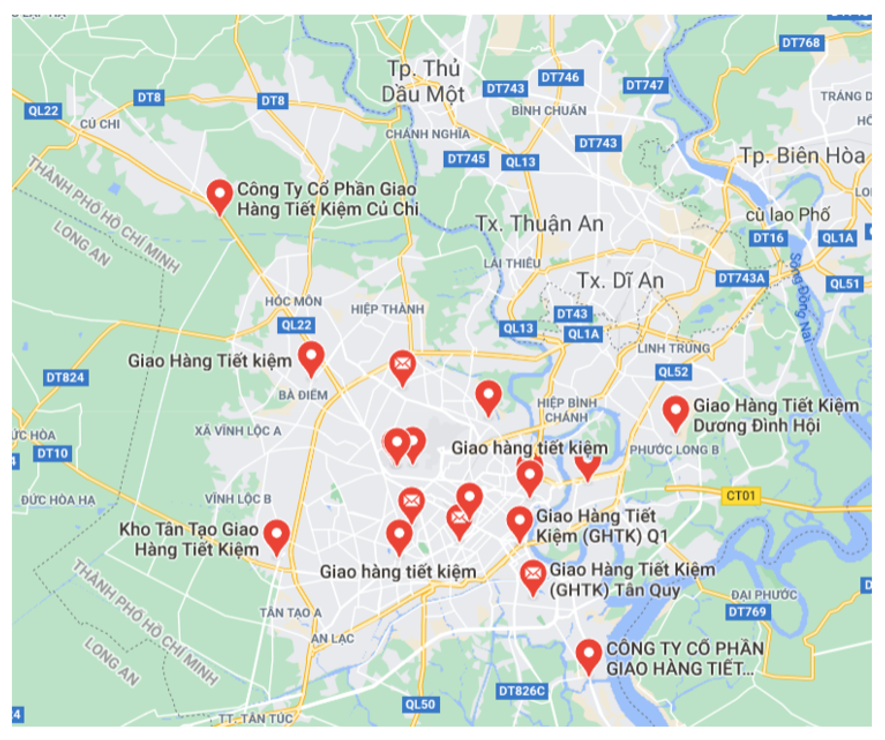
This section aims to evaluate the computational results of the ACO algorithm. The exact solutions obtained by CPLEX solver are also delivered to compare with ACO.

Table 1 shows the comparison between results obtained by the proposed ACO algorithm and CPLEX. For each instance, five runs have been considered in which minimum (Min), maximum (Max) value and average (Average) values are calculated to compare with the exact solution. The gap between them will also be retrieved to validate the solution quality proposed by ACO algorithm.

As it can be shown in the Table 1, the gap between the two methods is 1.16% on average based on three instance scales, although they are small-scaled instances, they can show the reliability on the method used for searching solution proposed by ACO algorithm is reasonable. It can easily solve the 6-customer and 10-customer instances with 0% gap. It shows that the solution quality of the proposed approach is extremely reliable for the small-sized problem where the requester set varies from 6–10. However, when the instances increase more slightly to 12, 16 and 18, the gap appears but insignificant, around 0.63–3.65%. Computational time on solving the problem by ACO is averagely around 22.78 s for the whole instance set while that of CPLEX is also around 23.78 s. They are approximately equal, however, when increasing the problem size, the time performance on the meta-heuristics approach is more outstanding which is a common strong point of meta-heuristics approach compared with mathematical approach. It is inevitable that the increase on the problem size can be the barrier to the solution quality proposed by ACO, however, tuning the parameter setting or changing the way search optimal solution in a more logical and intelligent way can have impact on the gap reduction, this point is quietly interesting to do the research to improve the proposed method. Besides, the evaluation on the practical features of the studied method will be shown in the Section 4.3 which solve real case study.

4.3. Case Study

In this section, the solution obtained by the ACO algorithm to the realistic case study are summarized. The problem is proposed by Giao hang tiet kiem company, one of the reputative E-logistics service providers in Vietnam.

Figure 3 depicts the warehouse network of the case study in Ho Chi Minh city obtained from Google map. However, only set of large warehouses are shown in the figure, there are still other sets of small warehouses. The company has totally 50 small and large warehouses and 1 depot located in the same city. The parameter settings for ACO algorithm and data setup form are similar to those in the small-sized instance. It employs set of heterogeneous vehicle fleet and policy on working duration of truck drivers which is limited below 9 h per driver per trip. In the warehouse network, there are some pickup nodes that play as the delivery destination of other pickup ones. Therefore, to guarantee the constraint of visiting each node exactly once, dummy node is created to indicate the number of visits on the specific node, the number of dummies created for each node implies the number of visits. Due to this modification, the number of requesters increases to around 1000 customers. However, it can still be solved by ACO and propose reasonable computational time which is around 900 to 1020 s. The summary of results when ACO is applied to the real case is shown in

Table 2. Summary of results when ACO is applied to real case.

Vehicle ID	Total Distance (m)	Total Time (h)	Capacity
28	181,683	3.29482	0.039473684
37	146,620	2.95774	0.043274854
44	269,635	5.28208	0.048245614
48	278,462	5.44326	0.083333333
22	273,706	4.92704	0.078654971
29	252,486	5.35718	0.017836257
33	155,872	3.19608	0.029532164
35	282,634	5.59536	0.603216374
41	145,496	3.17976	0.013157895
45	216,041	4.09412	0.043859649
23	197,074	3.96682	0.046491228
27	227,014	4.84774	0.066374269
2	243,202	4.61812	0.958
30	149,347	3.44958	0.047953216
39	190,161	4.1299	0.092690058
40	184,611	3.35338	0.034795322
46	277,438	5.32206	0.040350877
47	263,489	4.7877	0.497076023
49	253,517	5.39702	0.007309942
51	237,076	4.90112	0.104093567
26	255,230	4.85868	0.114619883
32	138,889	2.63174	0.005847953
34	279,517	5.91702	0.061988304
4	237,012	5.06692	0.852555556
36	277,189	5.0947	0.566959064
6	193,887	3.5942	0.629111111
8	145,858	3.187	0,850222222
38	109,955	2.46894	0,707894737

.

5. Conclusions

A variant of vehicle routing problem with time window was studied in this paper, some practical constraints were added to increase the applicable features for the study which are heterogeneous fleets of truck, working duration allowed and multiple pickups multiple deliveries consideration. Beside the mathematical model proposed to solve the problem, our research presents ACO algorithm, a meta-heuristics approach to attack large-scale problems. This study is useful for the consideration of time-window and heterogeneous constraints in developing the ACO algorithm because these constraints are even today challenging for the majority of methods known from the literature review. In addition, the solution quality of ACO approach can be proved that it is reliable to use by small gap between its obtained solution and that of CPLEX reported in the Section 4.2. Therefore, it can be reasonable to conclude that the solution proposed by ACO algorithm studied in this paper has high quality and reliability to apply in solving the proposed variant of VRPTW.

In future research, it might be worthwhile to analyze more optimal principles to search for an optimal solution by ACO or to combine ACO with another meta-heuristics to have a better solution. Besides, there are some more improvements that can be interesting and practical to develop, such as obtaining the dynamic distance and travelling time based on the current traffic dense and considering truck driver’s break time as a constraint in the model.

References

1. Toth, P.; Vigo, D. The Vehicle Routing Problem, 1st ed.; Society for Industrial and Applied Mathematics: Philadelphia, PN, USA, 2002; pp. 385–386. [Google Scholar]
2. Dantzig, G.B.; Ramser, J.H. The truck dispatching problem. Manag. Sci. 1959, 6, 80–91. [Google Scholar] [CrossRef]
3. Clarke, G.; Wright, J.W. Scheduling of vehicles from a central depot to a number of delivery points. Oper. Res. 1964, 12, 568–584. [Google Scholar] [CrossRef]
4. Montoya-Torres, J.R.; Lopez Franco, J.; Nieto Isaza, S.; Felizzola Jimenez, H.; Herazo-Padilla, N. A literature review on the vehicle routing problem with multiple depots. Comput. Ind. Eng. 2015, 79, 115–129. [Google Scholar] [CrossRef]
5. Jian, L.; Li, Y.; Panos, M.P. Multiple-depot vehicle routing problem with time windows under shared depot resources. J. Comb. Optim. 2016, 31, 515–532. [Google Scholar]
6. Solomon, M.M. Algorithms for the vehicle routing and scheduling problem with time window constraints. Oper. Res. 1987, 35, 254–265. [Google Scholar] [CrossRef] [Green Version]
7. Cordeau, J.F.; Desaulniers, G.; Desrosiers, J.; Solomon, M.M.; Soumis, F. The VRP with time windows. In The Vehicle Routing Problem; Toth, P., Vigo, D., Eds.; SIAM Monograp: Philadenphia, PA, USA, 2002; pp. 157–186. [Google Scholar]
8. Baldacci, R.; Bartolini, E.; Mingozzi, A. An exact algorithm for the pickup and delivery problem with time windows. Oper. Res. 2011, 59, 414–426. [Google Scholar] [CrossRef]
9. Furtado, M.G.S.; Munari, P.; Morabito, R. Pickup and delivery problem with time windows: A new compact two-index formulation. Oper. Res. Lett. 2017, 45, 334–341. [Google Scholar] [CrossRef]
10. Baldacci, R.; Toth, P.; Vigo, D. Exact algorithms for routing problems under vehicle capacity constraints. Ann. Oper. Res. 2010, 75, 213–245. [Google Scholar] [CrossRef]
11. Desrochers, M.; Lenstra, J.K.; Savelsbrgh, M.W.P.; Soumis, F. Vehicle routing with time windows: Optimization and approximation. In Vehicle Routing: Methods and Studies; Golden, B.L., Assad, A.A., Eds.; Elsevier Science Publishers: Amsterdam, The Netherlands, 1988; pp. 65–82. [Google Scholar]
12. Laporte, G. The vehicle routing problem: An overview of exact and approximate algorithms. Eur. J. Oper. Res. 1992, 59, 345–358. [Google Scholar] [CrossRef]
13. Chen, X.; Kong, Y.; Dang, L.; Hou, Y.; Ye, X. Exact and metaheuristic approaches for a biobjective school bus scheduling problem. PLoS ONE 2015, 10, e0132600. [Google Scholar]
14. Laporte, G.; Nobert, Y. Exact Algorithms for the Vehicle Routing Problem. N.-Holl. Math. Stud. 1987, 132, 147–184. [Google Scholar]
15. Faiz, T.; Chrysafis, V.; Md Noor, E.A. A column generation algorithm for vehicle scheduling and routing problems. Comput. Ind. Eng. 2019, 130, 222–236. [Google Scholar] [CrossRef] [Green Version]
16. Fisher, M.L. Optimal solution of vehicle routing problems using minimum K-trees. Oper. Res. 1987, 42, 626–642. [Google Scholar] [CrossRef]
17. Ropke, S.; Cordeau, J.-F. Branch and cut and price for the pickup and delivery problem with time windows. Transp. Sci 2009, 43, 267–286. [Google Scholar] [CrossRef] [Green Version]
18. Roeva, O.; Fidanova, S. Comparison of different metaheuristic algorithms based on InterCriteria analysis. J. Comp. App. Math. 2018, 340, 615–628. [Google Scholar] [CrossRef]
19. Ho, S.C.; Haugland, D. A tabu search heuristic for the vehicle routing problem with time windows and split deliveries. Comput. Oper. Res. 2004, 31, 1947–1964. [Google Scholar] [CrossRef]
20. Bowerman, R.L.; Calamai, P.H. The spacefilling curve with optimal partitioning heuristic for the vehicle routing problem. Eur. J. Oper. Res. 1994, 76, 128–142. [Google Scholar] [CrossRef]
21. Dondo, R.; Cerda, J. A cluster-based optimization approach for the multi depot heterogeneous fleet vehicle routing problem with time windows. Eur. J. Oper. Res. 2007, 176, 478–1507. [Google Scholar] [CrossRef]
22. Cordeau, J.F.; Gendreau, M.; Laporte, G.; Potvinand, J.Y.; Semet, F. A guide to vehicle routing heuristics. J. Oper. Res. Soc. 2002, 53, 512–522. [Google Scholar] [CrossRef]
23. Szeto, W.Y.; Wu, Y.; Ho, S.C. An artificial bee colony algorithm for the capacitated vehicle routing problem. Eur. J. Oper. Res. 2011, 215, 126–135. [Google Scholar] [CrossRef] [Green Version]
24. Dorigo, M.; Stutzle, T. Ant Colony Optimization, 1st ed.; MIT Press: Cambridge, MA, USA, 2004; pp. 305–315. [Google Scholar]
25. Bullnheimer, B.; Hartl, R.F.; Strauss, C. Applying the ant system to the vehicle routing problem. In Meta-Heuristics: Advances and Trends in Local Search for Optimization; Voss, S., Martello, S., Osman, I.H., Roucairol, C., Eds.; Kluver Academic Publishers: Boston, MA, USA, 2012; pp. 285–296. [Google Scholar]
26. Tan, W.F.; Lee, L.S.; Majid, Z.A.; Seow, H.V. Ant colony optimization for capacitated vehicle routing problem. J. Comput. Sci. 2012, 8, 846–852. [Google Scholar]
27. Doerner, K.; Gronalt, M.; Hartl, R.F.; Reimann, M.; Strauss, C.; Stummer, M. Savings Ants for the vehicle routing problem. Lect. Notes Comput. Sci. 2002, 2279, 73–109. [Google Scholar]
28. Ma, Y.; Han, J.; Kang, K.; Yan, F. An Improved ACO for the multi-depot vehicle routing problem with time windows. In Proceedings of the Tenth International Conference on Management Science and Engineering Management; Xu, J., Hajiyev, A., Nickel, S., Gen, M., Eds.; Springer: Singapore, 2018; pp. 1181–1189. [Google Scholar]
29. Zhang, X.; Tang, L. A new hybrid ant colony optimization algorithm for the vehicle routing problem. Pattern Recognit. Lett. 2009, 30, 848–855. [Google Scholar] [CrossRef]
30. Mazzeo, S.; Loiseau, I. An ant colony algorithm for the capacitated vehicle routing. Electron. Notes Discret. Math. 2004, 18, 181–186. [Google Scholar] [CrossRef]
31. Yu, B.; Yang, Z.Z.; Yao, B.Z. An improved ant colony optimization for vehicle routing problem. Eur. J. Oper. Res. 2009, 196, 171–176. [Google Scholar] [CrossRef]
32. Anh, P.T.; Cuong, P.T.; Ky Phuc, P.N. The vehicle routing problem with time windows: A case study of fresh food distribution center. In Proceedings of the 11th International Conference on Knowledge and Systems Engineering (KSE), Danang, Vietnam, 24–26 October 2019. [Google Scholar]
33. Bullnheimer, B.; Hartl, R.F.; Strauss, C. An improved ant system for the vehicle routing problem. Ann. Oper. Res. 1999, 89, 319–328. [Google Scholar] [CrossRef]
Figure 1. Flowchart of ACO Algorithm for MPMDVRPTWHF.
Logistics 05 00028 g001
Figure 2. Example of solution construction by the proposed ACO algorithm.
Logistics 05 00028 g002
Figure 3. A cut from google map of warehouse network of the case study.
Logistics 05 00028 g003