
An Extended Model for Disaster Relief Operations Used on the Hagibis Typhoon Case in Japan

1
Faculty of Logistics, Molde University College, 6410 Molde, Norway
2
Department of Business Administration, Western Norway University of Applied Sciences, 5020 Bergen, Norway
*
Author to whom correspondence should be addressed.
Logistics 2021, 5(2), 39; https://0-doi-org.brum.beds.ac.uk/10.3390/logistics5020039
Submission received: 13 March 2021
/
Revised: 27 May 2021
/
Accepted: 1 June 2021
/
Published: 16 June 2021
(This article belongs to the Section Humanitarian and Healthcare Logistics)
Abstract
:This paper presents a generalization of a previously defined lexicographical dynamic flow model based on multi-objective optimization for solving the multi-commodity aid distribution problem in the aftermath of a catastrophe. The model considers distribution of the two major commodities of food and medicine, and seven different objectives, and the model can easily be changed to include more commodities in addition to other and different priorities between the objectives. The first level in the model is to maximize the amount of aid distributed under the given constraints. Keeping the optimal result from the first level, the second level can be solved considering objectives such as the cost of the operation, the time of the operation, the equity of distribution for each type of humanitarian aid, the priority of the designated nodes, the minimum arc reliability, and the global reliability of the route. The model is tested on a recent case study based on the Hagibis typhoon disaster in Japan in 2019. The paper presents a solution for the distribution problem and provides a driving schedule for vehicles for delivering the commodities from depots to the regional centers in need for humanitarian aid.
1. Introduction
The tasks related to humanitarian logistics are a combination of logistics and humanitarian relief, focusing on maintaining health, life, and living conditions. They deal with transportation, storage, and transshipment, as well as the management of humanitarian aid focusing on logistics services and logistics costs. The logistics services objective ensures that aid is delivered to the people most in need as quickly and reliable as possible, while the logistics costs objective ensures the best possible service within a limited budget for the humanitarian relief [1]. Humanitarian logistics have their own specific challenges and difficulties depending on the type, location, and degree of disaster. In the case of acute severe natural disasters, people need to be rescued and taken care of within a short period of time. Lack of information, destroyed infrastructure, and limited international assistance are particular problems. Schumann-Bölsche [1] notes that in the case of persistent natural disasters, such as regular droughts in some regions of Africa and in case of political crises, the challenge is not so much related to the time aspect but rather focuses on limited financial resources and logistical potential, for example, in seaports or in refugee camps. Political and cultural issues can also complicate humanitarian logistics.
The World Heritage Encyclopedia defines humanitarian logistics as a branch of logistics that specializes in organizing the delivery and storage of supplies during natural disasters or complex emergencies to the affected area and people [2]. During the onset of a disaster, all elements of the system must work according to a proven, ready-made scheme based entirely on logistic principles. The challenge for the responsible authorities is to respond to the request as efficiently as possible and to minimize the response time, execution costs, and number of distribution centers involved. Mobilization centers and brigades are sent to the area for managing the delivery of food and organize rescue teams. The private sector and the field of humanitarian logistics can enrich each other, and the private logistics sector can learn from humanitarian assistance, e.g., in order to provide flexibility and speed in difficult conditions. Hence, it is valuable to simulate disasters in various scenarios in advance in order to take appropriate precautionary measures to prevent its occurrence or to assign all possible resources to minimize the damage. The importance of logistics in disaster preparedness is in line with observations, rehearsal, warning, and hazard analysis. However, in humanitarian supply chains, it is extremely difficult to assess the efficiency indicators accustomed to business logistics. The demand for such operations is very unpredictable. It is difficult to assess performance and to predict working conditions, and there is a lack of incentives for performance measurement and environmental research, as the domain is non-commercial. Depending on the nature of the disaster, transportation management for disaster relief can be complex. It depends on budget, coverage of demand, road reliability, equity of distribution, security in the disaster area, and other criteria [3]. One of the main problems of interest in disaster management deals with the distribution of humanitarian aid. The planning of such a distribution is done along different phases of the process, such as pre-disaster and post-disaster phases. In this work, we will focus on the post disaster humanitarian aid distribution. This implies that there exists some available information characterized by high uncertainty, such as demand, resources required, the state of the infrastructure, the time required to complete the operation, and the dispersion of resources. In addition, there is usually a high time pressure and a short period of time to prepare and run the model. One of the objectives of this study is to investigate and create a realistic case study based on a recent disaster. Further, this work aims at developing a realistic mathematical model for the problem and to use the case study to assess the performance of the built model. In this context, the problem consists of designing a realistic distribution schedule within the available resources, taking into account several efficiency criteria.
2. Literature Review
The humanitarian sphere is unique for the implementation of any theory. Therefore, in their studies, Guide and Van Wassenhove [4] emphasize that at the time of an emergency, decision-makers have to work in conditions of limited information and time. It follows that using models that require considerable searching time and a large amount of input data is not the best solution in such cases. They also note that data collection will be a rather complicated procedure, and all the same, the received data will most likely be of poor quality [4,5]. Nevertheless, some researchers have succeeded in developing models successfully applied in humanitarian logistics. In 2009, inspired by experience, Carroll and Neu [6] described the state of humanitarian logistics as unstable with a huge number of participants, which creates unpredictability and asymmetry. They developed a modern model covering all aspects of logistics and narrowed the gap between the current and necessary, flexible state of humanitarian logistics. They also proposed several universal methods that, in their opinion, lead to “flexibility of cooperation and efficient logistics for responding to natural disasters, which will lead to sustainability and universality”. The vast majority of humanitarian logistics research focuses on the preparation and planning stages, as well as applied policies and procedures. The studies that develop specific models mainly propose to introduce information technologies into the supply chain. For example, in 2002, a knowledge management framework serving as a tool for decision makers during a humanitarian operation was developed. It is argued that such a system is self-learning and the more information it accumulates, the better it will work in the future [7]. The applicability of the research to the practical side of real life is very important. If the research cannot be used in practice, the importance of such work is immediately devalued. If repeated over and over again, this may lead to a decrease in the need of practitioners for the work of scientists as a whole [5].
2.1. Research on Humanitarian Logistics
The field of humanitarian logistics can include a wide range of logistic problems. One important approach is operations research and quantitative methods for finding the best possible solution under some given criteria. Within this field, vehicle routing problems play a crucial role, and Anuar et al. [8] have published an extensive survey on vehicle routing in humanitarian operations. The survey classifies papers based on attributes for application, disaster type, model characteristics, and solution approach.
The UCM-HUMLOG research group [9] at the Complutense University of Madrid is focusing their research on development of decision support systems for meeting logistical problems in disaster management. The article by Vitoriano et al. [10] aims to identify relevant differences in disaster management compared with other types of logistics. They introduce a model for assessment of consequences in the early stage after a disaster and another for the last mile distribution of humanitarian aid focusing on the multicriteria nature of such problems. The multicriteria approach is further developed by Mejita-Argueta et al. [11], who looked specifically into preparedness of frequent and foreseeable floods. They considered the three criteria of evacuation and distribution time and the total cost of the operation. In an earlier paper, Vitoriano et al. [12] presented a goal programming-based humanitarian aid distribution system focusing on specific transport problems appearing in humanitarian aid distribution. Another approach is a lexicographic goal programming model presented by Flores at al. [13], focusing on evacuation and the objectives of the number of evacuated people, the operation time, and the cost. The model is evaluated through a case from the earthquake and tsunami that hit Palu, Indonesia, in September 2018. Location of facilities is another concept relevant for disaster response planning. Rennemo et al. [14] presented a three-stage model considering opening of local distribution facilities, allocation of suppliers and last mile distribution of aid. The model is stochastic with respect to the available vehicles, the state of the infrastructure, and the demand. Monzon et al. [15] developed a pre-disaster model with uncertainty and multiple criteria for facility location and network fortification. The model is a two-stage stochastic model where the first stage concerns decisions to be taken before the disaster strikes, such as location of inventories and fortification of road sections. The second stage relates to the situation after the disaster has struck and solves the problem about distribution of goods in the current network. The methodology was tested on a case based on the storm that hit Mozambique in 2018.
Distribution problems in disaster management are often defined by multiple criteria and high complexity under uncertain conditions. Hence, larger instances will not always be possible to solve to optimality in real-time, and heuristics might be necessary for finding acceptable solutions. Ferrer et al. [16] developed a constructive algorithm and a GRASP metaheuristic for solving a last-mile distribution problem and tested the algorithm on a case study based on the 2010 Haiti earthquake. The same authors presented a few years later an ant colony-based methodology [17] for the same problem applied on case studies from the Haiti earthquake together with another case based on the 2005 Niger famine.
2.2. The Hierarchical Compromise Model
Liberatore et al. [18] proposed a hierarchical compromise model for the joint optimization of recovery operations and distribution of emergency goods based on a multi-criteria solution approach and a three-level lexicographic optimization method. This model focuses on recovery of damaged arcs in post-disaster operations. It calculates which temporary emergency access roads, proper roads, tunnels, or bridges that need to be restored or cleaned in the first place to open a path through them. In addition, it shows how to do this with minimal loss of time and minimum budget costs while fully satisfying demand and covering all affected areas and sites. The emphasis is on restoration work rather than a distribution plan, so it is assumed that the capacities of the distribution centers are unlimited and the distribution of products is continuous.
The hierarchical model implies that the highest priority is to maximize the satisfied demand for humanitarian aid and to help people in a catastrophe, while subsequently other criteria are taken into account. In their paper, Liberatore, et al. [18] consider optimization criteria such as maximum service time, total demand in the entire considered area, maximum ransack probability during the delivery of goods along the selected route and the minimum reliability of roads on the selected distribution plan. The first level of the lexicographic model computes the maximum demand to meet and which routes to use, taking into account all the above criteria. At the second level, the model optimizes each criterion individually by minimizing the maximum of normalized criteria deviations from ideal values with the previously found total demand value already fixed, using Chebyshev distances. At the third level of lexicographic optimization, optimal solutions are selected from a variety of alternatives. To accomplish this, researchers use the method of minimizing the weighted sum of the normalized deviations of the criteria without losing the results achieved at previous levels. Liberatore et al. [18] emphasize the need to coordinate services involved in restoring transport infrastructure and humanitarian aid delivery services. Moreover, they empirically prove this by conducting an experiment by replacing the three-level solution described above with three independent sequential models. This, in the same way that two separate services would make their decisions without coordinating their actions but working separately. The “gaps” between the sequential solution and a coordinated one show how important cooperation between rescue services is when disasters occur, as well as the power of reliable information.
2.3. Dynamic Flow Model
A subsequent study on the current topic was conducted by Tirado et al. [19]. They proposed a dynamic flow model for solving the aid distribution problem in emergency situations based on a multi-criteria approach and a lexicographic method of goal programming. In their work, Tirado et al. [19] proposed a model focusing on building a realistic distribution plan for last mile delivery, assuming that the resource allocations and transport infrastructure are known. For solving the problem, they introduced a time horizon, divided into periods of one minute each. This approach allows for a realistic distribution schedule. The dynamic model permit vehicles to follow different routes to visit the same node and to visit a node several times. At the same time, the statically model does not imply such optimization.
The decision-making process takes place at two lexicographical levels where four criteria—the global distributed quantity, operating time, aid distribution equity, and cost—are taken into account. The primary goal of the model is to maximize aid for people in need, and this is directly proportional to the amount of demand that should be satisfied. The objective function of the first stage is to allocate the planned amount of resources within the available budget, when, at this level, no trade-offs with other optimization criteria are permitted. At the first stage, the solution obtained is integer. It does not require a high computational effort and hence it is calculated quickly. The second lexicographical level of the model determines the distribution schedule, considering the remaining goals. The decision maker, as an expert in the field, can specify the weights of each criterion. However, by default, preference is given to minimizing the execution time of the operation, and then secondly comes the cost and equity. For a dynamic model, it is important to correctly define the length of the time horizon given as the maximum number of time periods. This is important for the model to be able to optimize not only the time criterion but other criteria as well. Otherwise, the time horizon can be limited in such a way that the other criteria will not have any implication since they directly depend on the time of the operation in real life. However, for modelling, it can be determined approximately or experimentally by running the program and checking the results. If a reasonable solution is found within a given time horizon, then the time horizon was chosen correctly, but if not, one could make it longer and run the model again. However, another option used by Tirado et al. [19] is to use the execution time of the operation found by solving the static flow model defined by Ortuño et al. [20], increased by 10%.
After testing, the dynamic model shows a slight increase in response time and cost, due to separation of the time horizon into periods, but at the same time, it creates a realistic schedule for the distribution of humanitarian aid, allowing for multiple departures from each node. This schedule allows more people to get help earlier, although their need may not be fully met immediately. In the end, however, the demand will be satisfied by the next vehicle that follows the route. Difficulties in solving such a model may appear when the time horizon increases. This will lead to a problem of high dimensionality, which may require the use of extensive computer power to obtain a solution within reasonable time.
2.4. Compromise Programming Model
In a recent study, Ferrer et al. [3] present their newest application for humanitarian logistics. The application is based on a compromise-programming model for multi-criteria optimization in humanitarian last mile distribution. They argue that it is the first model in its field capable of optimizing many criteria at the same time, while creating a realistic schedule for vehicles and, if necessary, forcing them to travel in convoys. The model proposed is intended to help in the distribution of humanitarian aid after a disaster, meaning that the information involved in the decision-making process contains a high degree of uncertainty. Despite this, it is a deterministic model where Ferrer et al. [3] assume that the parameters entered for the computation will consider the uncertainty of the current situation. The model builds on the compromise programming method considering six criteria, such as time, cost, priority, equity, security, and reliability. The approach ensures that the obtained solution is a non-dominated or efficient one, hence making sure that there is no other solution surpassing or equals the proposed solution in all criteria. Such a solution is as close to the ideal values as possible, within the available resources in the current situation. Ideal values are determined by solving the model individually for each criterion, without considering the importance of the others. It also implies that the decision maker already has an initial amount of information sufficient for designing the mission, e.g., the available amount of aid to be distributed and the number and type of vehicles available. The developed model is designed for the delivery of a single commodity, but it may be a tool with a diverse selection of goods pre-formed at the warehouse. The model makes an individual schedule from the supplier to the demand nodes for each vehicle, calculating the type of vehicle needed for a particular route. Furthermore, one can set the condition that the rescue organization does not have the necessary type of vehicles in its fleet, and in this case, the model can take into account rental of vehicles and calculate the optimal plan for such a scheme. At the same time, the model allows for constructing an operation for several depots and several types of vehicles considering the time of loading and unloading of vehicles and allowing for transshipment and split delivery. In addition, there are restrictions on the compatibility of certain types of vehicles with certain roads. Hence, a large vehicle cannot be assigned to a narrow rural road and so on. If an efficient solution requires the use of an unreliable arc, the model can append a convoy and police escort for this route, increasing the cost for the operation. Consequently, the use of unreliable arcs would be avoided if the other criteria allow for it. It may happen that there are nodes in hardly accessible locations, leading to the model bypassing them when finding a solution. In this layout, however, it is possible to designate such nodes as priority.
Given all of the above, it is easy to conclude that when using the model in real cases, the problem will have a high dimension, since a large number of variables is used in the calculations. Ferrer et al. [3] states that in order for the model to provide a fast enough solution, they had to use simple heuristic methods abandoning local search-based metaheuristics and complex evolutionary algorithms because they would require a very high computational effort. They applied the GRASP method [21], which is widely used for compromise optimization problems for finding good solutions. Although several researchers have focused on humanitarian logistics during the last years, the research field is still young. Hence, models developed are often insufficient for meeting the complex requirements in a real-life problem. This research is following the direction from Ortuño et al. [20] and Tirado et al. [19], starting with a static model and continuing with a dynamic model divided into time periods. The main innovation in this work is to generalize the model to include more than one type of product. In addition, more objective functions are considered, including the reliability of routes and potential priorities, and a new case study is presented for testing the model with real-life data. Such a model can be included in a decision aid system to be used when disasters appear.
3. Model Description
The model presented in this work is an extended version of the model developed by Tirado et al. [19]. In the basic model, such extensions were added as the ability to carry out multi-commodity delivery, the ability to determine the priority for all desired demand nodes, and two criteria for road reliability. The first criterion was maximizing reliability based on the worst arc used in the distribution route, while the second criterion aimed at maximizing reliability based on all arcs used in the operation. The ability to calculate travel time as a maximum between the speed limit of the road used and the speed characteristics of the vehicle traveling along it was also added. The presented model includes the possibility to adjust the length of the time period depending on the preferences of the decision maker. This option is convenient when planning long operations. Since the indicator for effective performance of the model is the execution time of the program, a large number of time periods will lead to a significant increase in the number of alternative solutions, making the response time of the model larger. Hence, the length of one time period should be chosen in a way that the response time of the model is reasonable and the quality of the provided distribution plan and schedule is adequate.
Vitoriano et al. [22] applied the priority condition on the model for humanitarian operations. The distinction exists in the fact that the authors implement the criterion of a priority node, while in the model presented in this work, priority can be given to several nodes at once in the same or different degree, depending on the choice of the decision maker. Such a formulation not only allows for assigning priority to several nodes at the same time but also allows the priority criterion not to conflict with the equity criterion for optimizing them simultaneously. Ortuño et al. [20] also considered a reliability criterion in their paper. However, this criterion is different from the one proposed in the current paper. The model, proposed by the Ortuño et al. [20], assumes the use of a security criterion based on the probability of robbery along the route, and the authors conclude that the ransack probability can be reduced and the relevance of the safety attribute improved by traveling in a convoy. In connection with this feature of the model, the reliability criterion is also calculated for a convoy traveling through an arc. However, in the presented case study, related to the humanitarian operation in Japan, there is no sense in applying a safety criterion based on the probability of being ransacked and overloading the model. The fact that a vehicle can move independently and not be guided by a convoy allows it to be more maneuverable and mobile. This leads to the fact that the vehicle can overcome its route faster, which is an undeniable advantage for humanitarian operations. When traveling in a convoy, the speed of all vehicles must be taken into account. If a situation where the speed characteristics of the vehicles are different occurs, then the entire convoy is obliged to move at a speed not exceeding the maximum speed of the slowest vehicle. This can significantly degrade the performance of the time criterion for long operations.
Goal programming turned out to be the most convenient method for obtaining the desired result, and therefore it was used as the main optimization method for our model. However, the model is formulated in such a way that adding more criteria to the objective function makes the boundaries of the importance of the criteria less evident.
The notation for the model is presented in Table 1, Table 2, Table 3 and Table 4, while the mathematical formulation is presented after the notations:
The model has to satisfy the following hard constraints:
Constraints related to load:
Constraints (1) are the dynamic load flow conditions ensuring that the load of each product at each node and time period is in balance. Constraints (2) make sure that distributed and stored load at the end of the operation is equal to the available amount of aid, while constraints (3) indicate that load variables should be non-negative, and, in our case, they should be integer.
Constraints related to travel time:
Constraints (4) compute travel time as the maximum number of time periods required to cross the arc, considering the speed limit of the arc and the speed characteristics for the vehicle type, selecting the lowest value to be used. The time measure parameter is introduced as a tool to manipulate the length of one time period. In this particular model, which means that one period of time is equal to 5 min.
Constraints related to vehicles:
Constraints (5) create the balanced flow of vehicles, taking into account the chronological sequence of time periods, the number of products to be delivered to the node, the type of vehicle, and the number of available vehicles in each node at a particular period of time. At the same time, constraints (6) ensure that only accessible vehicles are used for transportation. The inequalities (7) indicate that vehicle variables should be integer and non-negative.
Constraints related to vehicle-load:
Conditions (8) limit the sum of the carried products, ensuring that the vehicle capacity is not exceeded.
Cost conditions:
Equation (9) defines how the cost is calculated. The model assumes that the vehicles return empty to their original point, in other words, they drive twice through the same route. The fixed cost includes all expenses that do not change throughout the operation, such as renting a vehicle, salaries of drivers, and coordinators of the operation. These components are directly dependent on the type of vehicle. The variable cost includes loading/unloading charge for each type of product and fuel consumption. Total costs depend on the total travel distance, the selected routes, the number and type of used vehicles, and the amount and product ratio of distributed aid. Condition (10) bounds the total costs for the operation by the budget limit. This should not be exceeded, although a desired target could be defined by the decision maker.
Load conditions:
Constraints (11) ensure that the maximum amount available of each product planned for the operation is not exceeded. Parameter represents the target of the global amount of aid to be distributed.
Equity conditions:
In the previously presented models, the authors did not consider such criteria as the equity of multicommodity delivery. Therefore, the proposed approach to calculate the fairness of the distribution of goods between nodes was different. After conducting a series of experiments, we can conclude that the Min-Max goal programming approach provides the most even distribution plan for multi-product cases.
Thus, constraints (12) show the maximum inequity among the nodes and thereby measures how equitable the distribution plan is in relation to food. Constraints (13) compute the maximum inequity among the nodes in relation to medicine and thereby measures how equitable the medicine aid is distributed. Using these constraints, the model computes the largest proportion of unsatisfied demand by product among the nodes. The criteria take values of real numbers between 0 and 1, so the variables are equal to 0 if demand of all nodes for the specified product is completely fulfilled and positive otherwise. According to the goal programming methodology applied in this model, any target cannot take a zero value . Therefore, the target of the equity criteria will be a very small value close to zero.
Time conditions:
Operation time measure:
In order to deal with the operation time, two measures are introduced. Conditions (14) represent the number of time periods required to complete the operation. As mentioned earlier, in this case, a single period of time is equal to 5 min. The target value for the time criterion will be the number of periods during with which it is desirable to complete the operation.
Time Penalty measure:
Equation (15) adds a high penalty to long operations. The target value for the time penalty variable can be set based on how important it is to reduce the time of the operation, compared with other criteria in the model. If it is necessary to prioritize the criterion, then the target value for the variable can be extremely small and close to zero . If the time criterion does not take priority in the planned mission, then the goal for the may be equal to the target of the criterion (). Both variables turn into 0 if their corresponding goals are achieved and they get positive values otherwise.
Auxiliary constraints in relation to time-vehicle:
Binary variables takes value 1 if load has been delivered in period , and 0 otherwise. Hence, they show how many periods were used for the operation. Constraints (17)–(20) ensure that the binary time variable is defined correctly. Equation (16) computes the total number of available vehicles of each type in the network and works as a bound for constraints (18)–(20).
Priority condition:
Priority appears as a demand satisfaction criterion at specific nodes. Equation (21) weights the sum of the corresponding unmet demand overall demand nodes by their priority level. Such a criterion in a model designed to optimize the distribution plan for post-disaster operations can play a crucial role when the primary goal is to evenly deliver the aid between the nodes. However, the decision maker would know whether there are difficult accessible regions in unreliable areas of the network. In such cases, the model may discard solutions with a lower cost or a shorter operation time, in favor of a solution where the cost and time attributes deteriorate slightly but allow for more delivery to the indigent settlements. The target of the priority criterion can be a very small value close to zero, or any other value that the decision maker considers appropriate for a particular mission. The priority criterion takes the value of 0 only if the demand of all prioritized nodes is completely fulfilled, and it is positive otherwise.
Minimum reliability measure:
Natural disasters severely affect the viability of many aspects of the life of the affected people. The obvious fact is that disasters have a significant destructive impact on the transport infrastructure; hence, one of the most important criteria in the design of a humanitarian logistics model is reliability. It is necessary to take into account the fact that the degree of destruction of road infrastructure is uncertain after the disaster. One way to simulate this type of uncertainty is to conduct a reliability analysis. In this model, the reliability measure is defined through the probability of traversing a route successfully. More precisely, the reliability parameter is the probability indicating the safety of the arc. The probabilities are determined separately for each link of the transport network.
Criterion (22) states that the least probable arc in the distribution plan is the maximum reliability measure. In other words, it shows the probability of the most unreliable arc used to perform the operation.
Global route reliability measure:
Condition (23) reflects the global route reliability measure, which is computed as the product of all the probabilities among the set of arcs used in the operation. Such an equation assumes that all arcs are independent and have a specific reliability value. In order to linearize this expression, the logarithm is applied. Hence, criterion (24) significantly helps to increase the reliability of the full route, taking not only the lowest value in any link into account but also the remaining links throughout the route. The target value of the criterion should be determined based on knowledge that the value is represented by the logarithm. Accordingly, the target might be equal to . However, applying the realism of the constructed model, we assumed that all the links used are reliable and have a probability of 0.95. Additionally, considering the number of arcs in the presented case and assuming that at least half of the arcs in the existing transport network will be used to build the optimal solution, the following conclusion was made. Under ideal conditions, the product of all the probabilities for a realistic solution, that is, the global reliability along the entire route, will be less than or equal to 0.30. Thus, as a target value, there is no need to set a value other than and ask the model to achieve unattainable goals. At the same time, it is worth noting that the goal programming objective function is formulated in such a way that targets cannot be negative values. Consequently, the goal condition for the criterion (39) is set to avoid negativity while maximizing the desired criterion. As the result, the target of the criterion should be set equal to 1.2. Despite this reasoning, in any other operation, decision makers can be guided by their own considerations and determine other target values for the criterion.
Auxiliary constraints in relation to arc-vehicle:
The constraints (25) – (28) are introduced to guarantee that the binary variables are defined correctly. Condition (29) states that these variables are binary only taking values 0 or 1.
The goal constraints are defined as follows:
First level: primary goal:
Equation (30) is the load condition for the first level of the model. Parameter qp represents the total amount of aid desired to be distributed. The equation assures that at the end of the operation the sum of delivered goods in all the nodes that have a demand for a particular product should be equal to the quantity of products planned to the distribution, summarized over all products. If the condition is not fulfilled, then a positive value, equal to the amount of aid that could not be delivered, will be assigned to the deviation variable . If the condition is satisfied, the variable will be equal to zero.
Second level: load goal constraint:
This constraint is applied to designate the load condition at the second level of the model. After the value of the load deviation is determined, the variable is no longer involved in the calculations. It is replaced by the parameter , which fixes the value of the load deviation for the load condition of the second level. Thus, it can be noted that constraint (31) differs from constraint (30) only by parameter , which is determined by solving the primary goal. Otherwise, the constraint performs a similar function in the model.
Cost goal constraint:
The presented Equation (32) is used to limit the total cost to a desired target. By default, we already have a boundary for costs in terms of budget. However, from the real-life point of view, the goal is not only to keep costs within the available budget but also to find the cheapest possible solution fulfilling the given criteria. Hence, the target value for the cost condition can be set to any reasonable amount, e.g., 50% of the budget or similar, according to the decision maker.
Equity goal constraints:
The conditions (33) and (34) serve to indicate the goal for equity in the distribution of each type of product in the humanitarian operation. Specifically, they indicate that the maximum deviations between delivered load and demand should be minimized.
Time goal constraints:
The goal constraints (35) and (36) are formulated such that the time of the operation is minimized as much as possible.
Priority goal constraint:
Since the priority criterion reflects the unsatisfaction of demand for the prioritized nodes, the priority goal constraint (37) aims at minimizing this value.
Reliability goal constraints:
Equations (38) and (39) are the goal constraints for the reliability criteria. The constraints state that the reliability values should be maximized. The corresponding deviation variables will serve to compare obtained reliability values with the target values.
Equation (40) indicate that attribute variables should take non-negative values. An exception is the global route reliability criterion, , since it takes a logarithmic value, and the natural logarithm of contains non-positive values.
The final model is based on a two-phase solving method, known as lexicographical goal programming. The mathematical formulation of the objective function is written in Equation (41).
There are different opinions about the strengths and weaknesses of this method. However, relying on the studied literature it can be concluded that it is one of the most common methods for solving this kind of problem, alongside scalarization, Pareto optimization, and compromise programming. At the same time, studies have shown that compromise programming and goal programming provide the most relevant methods for multi-criteria optimization. A survey conducted by Jones and Tamiz [23] shows that in the case of using goal programming to solve real problems, most of them were solved using the lexicographic approach. Additionally, a while ago Romero [24] performed a research in which he proved that most of the flaws of the lexicographical goal programming methodology arise due to an incorrect application. In fact, some properties of the method, interpreted as disadvantages, can turn into advantages for problems in real life.
The first level model:
The lexicographic goal programming model considers two priority levels. For humanitarian distribution operations, the primary goal is delivery of the planned amount of aid to the affected population. However, conditions such as a budget, the number of vehicles available, or a short time horizon may lead to the objective being impossible to achieve. Therefore, as suggested by Tirado et al. (2014) [19], the first level of the model aims to determine the maximum total quantity of goods to be distributed under the existing restrictions. For this purpose, the desired quantity of products to be delivered is set as the target (30), and the model calculates whether it is possible to distribute the entire desired amount of aid or eventually finds the minimum possible deviation from the target. At the first level of the lexicographical model, the remaining goals defined for the mission are not considered, although their constraints are included in the model. Hence, the objective function of the first level is to minimize the deviation of the load criterion . In an ideal case, this should be equal to zero.
Equation (42) shows the model formulation for the first level solution, the objective function, and constraints to be included. Once the first level of the model is solved, it is determined how much of the global load can be distributed with the available set of resources, and we know the load deviation value that must be fixed in order to proceed to the second level of solution.
To continue the solving process, the objective function of the model is replaced by the one shown in expression (43) Constraint (30) is replaced by constraint (31), and further, the remaining goal constraints from (32) to (40) are added to the resulting model, as shown in expression (43).
In our case, the goals are not represented in the same units of measurement, so the normalization method should be implemented in the objective function by dividing each deviation variable by the corresponding goal to obtain normalized units for each criterion. Such a manipulation allows one to work with a percentage expression of satisfaction for each goal. In addition, the criteria can be assigned their own weight, showing the importance of one criterion compared to others for the decision maker. Weights can be set subjectively or by experimental selection after several runs of the model and evaluation of the results. Ultimately, the model calculates and minimizes a weighted sum of all goal deviations for each criterion except the load. One limitation of this model is that the time schedule might not be realistic. Using vehicle speed and road limits is not always sufficient to simulate the actual time in a real-life scenario, in particular when the time periods are as small as five minutes. The times for loading and unloading of vehicles are not included in this case study, even if the model can be extended to include such aspects. Real-life problems are always more complex and uncertain than theoretical case studies, but this model should be a step towards a realistic model to be used when sudden disasters appear.
4. Case Description
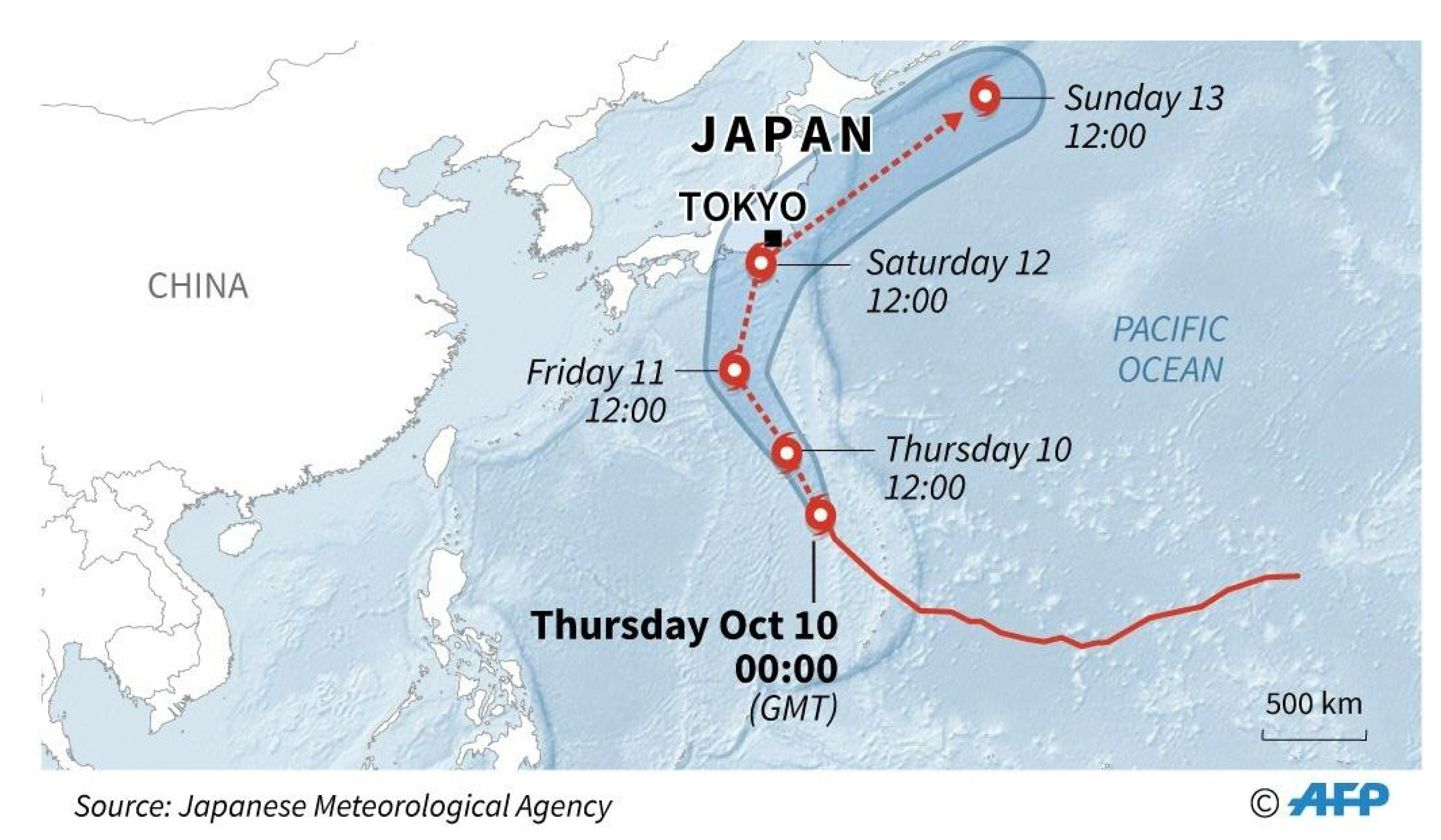
Humanitarian operation research needs realistic test cases to replicate experiments, validate models, and compare results. However, getting realistic data on humanitarian operations is challenging [25]. Confidentiality agreements or high acquisition costs discourage data sharing within the humanitarian operation research community. The realistic case study collected and presented in this work aims to benefit the humanitarian operation research area and have a positive impact for practitioners and beneficiaries. The case study is based on one of the recent disasters that shook the world—the typhoon Hagibis (meaning fast) that hit Japan on 12 October 2019. The typhoon was an extremely violent and large tropical cyclone that caused widespread destruction across its path, starting from October 6 up until 13 October 2019. Japanese meteorologists call it the most destructive in 60 years. This was the 38th depression, 9th typhoon, and 3rd super typhoon of the 2019 Pacific typhoon season. It was the strongest typhoon in decades to strike mainland Japan, and one of the largest typhoons ever recorded at a peak diameter of 825 nautical miles (1529 km). It was also the second costliest Pacific typhoon on record, with a damage estimated to 15 billion USD, only surpassed by the typhoon Mireille in 1991 (when adjusted for inflation). In addition, Hagibis was also the deadliest typhoon to hit Japan since 1979, with at least 98 fatalities, and it caused catastrophic destruction in much of eastern Japan. As shown in Figure 1, the typhoon passed through the most densely populated part of Japan, including the Tokyo metropolitan area, with more than 37 million residents and about 6000 people per square kilometer. The Typhoon spilled the river Tamagawa and caused much damage in its area. More than half a million people were forced to leave their homes, and the most severe damage was caused to agriculture and the infrastructure of nearby cities. The storm ripped through a wide area of the country, cutting off electricity and water supplies, causing mudslides, and flooding tens of thousands of homes [26].
Case Study Data
One of the most important issues in research is the ability to find relevant and appropriate data. The data for compiling this case study were obtained from secondary sources on the Internet. Emergency Response Coordination Center has published a comprehensive report illustrating the most destroyed territories and describing the overall situation on 14 October 2019 [27]. Data such as the number of casualties and the population density were obtained from the official website of the Statistics Bureau in Japan [28] and from a website of statistics separately for each prefecture of Japan [29]. Based on these data, the estimated amount of aid needed for distribution has been calculated. The Japan Meteorological Agency [26], United Nations Office for the Coordination of Humanitarian Affairs [30], and NGO Japan Platform [31] provided information regarding the typhoon characteristics, its consequences, and post-disaster response methods. Information about damaged railway lines and areas of damaged roads was obtained from Ministry of Land, Infrastructure, Transport, and Tourism of Japan [32], which led to the choice of road transport. From UNOCHA [33] and EMDAT—International Disaster Database [34], archived data about international disaster experience was collected. In addition, services such as OpenStreetMap, Yandex, and Google Maps were used to properly compose the road network. As mentioned above, the humanitarian distribution network was built for the Tokyo Prefecture and its surroundings, so that humanitarian aid would be delivered to the ten regional centers of Fujisawa, Funabashi, Kasukabe, Kawagoe, Kawasaki, Hachioji, Kofu, Saitama, Chiba, and Tokyo. The aid should be distributed through the transportation hubs at Haneda Airport, Narita Airport, Yokohama Port, and a distribution center specializing in nutrition located at Tsuchiura. The following characteristics of the transport network are provided. The transport network consists of 10 demand nodes, 4 supply depots, and 58 available connections between locations. The humanitarian aid to be delivered is divided into two categories, namely, food and healthcare products including medicines, but the model could easily be extended with more commodities. Assuming that about 10% of the city’s population needed aid, the total demand for food was estimated to 2585 tons for food and 440 tons for healthcare, making the desired amount of humanitarian aid to be distributed 3025 tons for the whole operation. This is based on approximately 2 kg. in total per person where almost 15% consisted of healthcare products. The depots are based in places where humanitarian aid is delivered, in this case two airports, one seaport, and one large distribution center with high capacity. The first depot is at Haneda Airport with 1100 tons of food and 200 tons of medicine available, and the second depot is Narita Airport with 440 available tons of food and 80 tons of medicine. Then follows the third depot at Yokohama Port with 230 tons of food and 80 tons of medication available, and at last the distribution center at Tsuchiura with 1270 tons of food available for distribution. Hence, the total amount of humanitarian aid available was 3040 tons of food and 360 tons of medicine, making a total of 3400 tons. This was sufficient to meet the demand for food, but a shortage of 80 tons for medicine at the demand nodes remained. The summary of the relevant data is shown in Table 5.
To perform the operation, three types of vehicles with different capacities are used. They are categorized as small vehicles with a capacity of 5 tons, medium vehicles with a capacity of 15 tons, and large vehicles with a capacity of 25 tons. Moreover, 119 small, 81 medium, and 44 large vehicles are available for transportation, making a total of 244 vehicles. Table 6 reflects vehicle characteristics such as capacity, maximum speed, fixed costs per kilometer, and variable costs depending on distance, cargo amount, and type of product being transported. The model proposed in the previous section of this paper provides the ability to give priority to some nodes. Based on a number of experiments explained later, priority was given to the city of Kofu, node N7, located in an arduous area, and to the city with the greatest demand—Tokyo, node N10. The planned mission consists of distributing the desired amount of humanitarian aid within the available budget of US$1,000,000.
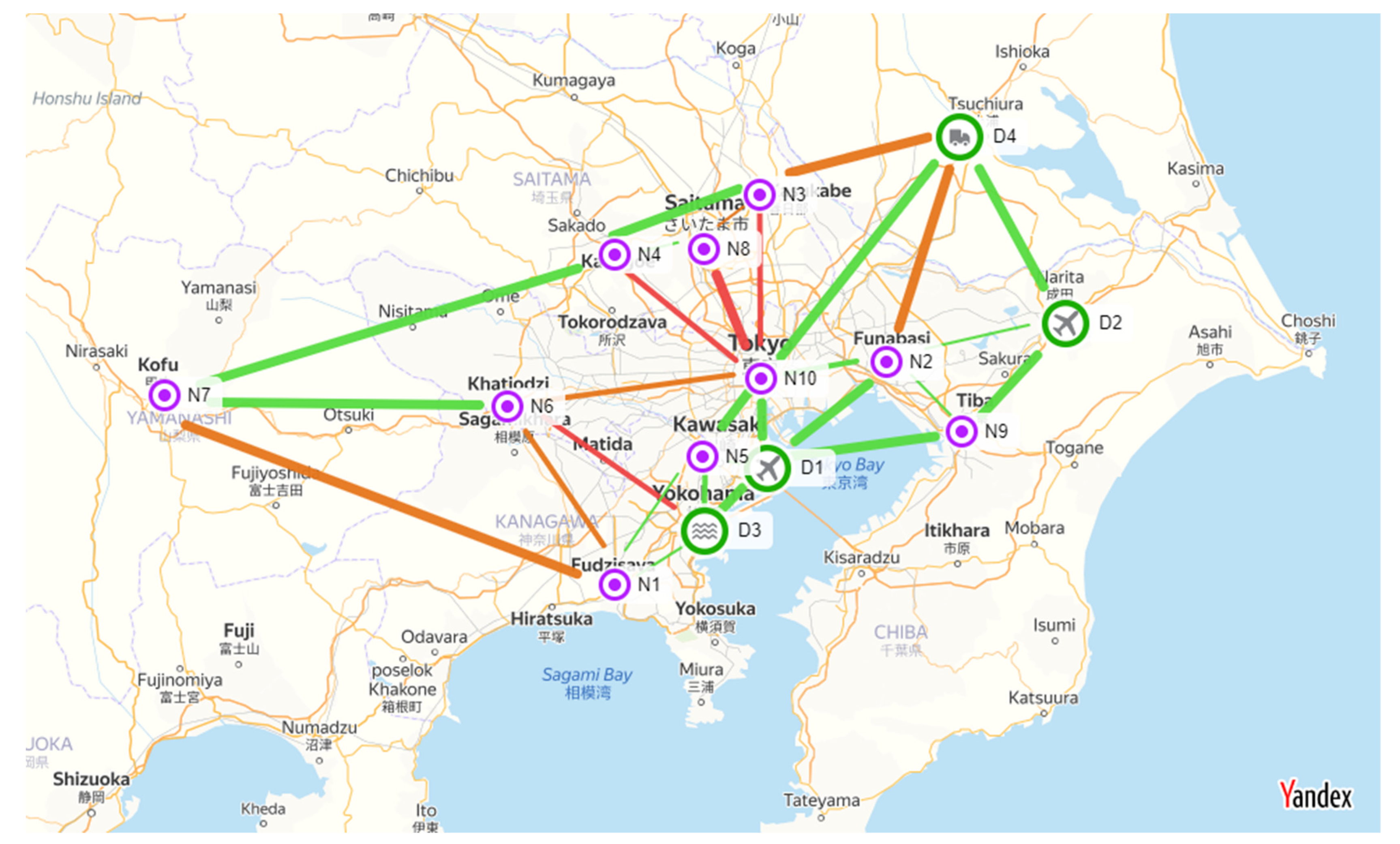
Figure 2 presents the transportation network with labelled demand nodes, supply depots, and links that reflect the distance, speed, and reliability of roads available for transportation. The links are shown in different colors depending on the reliability of the arc. Green color represents a reliable arc where the probability of traversing the arc is over 70%. The orange color represents an arc with a probability more than 50%, while the red color indicates that the probability is less than 50%. The different thickness of the links shows the quality of the road. Hence, the thicker the arc, the higher the maximum speed of its passage.
Information on the distance and maximum speed of the road was collected from Google Maps and Open Street Maps. These sources provide comprehensive information about the type of road and their quality. Reliability data for the links are the result of conclusions based on the reports of MLIT [32], on the extent of destruction of certain routes, as well as on the report of Reliefweb [27], which provides the map of destruction showing the epicenters of the destroyed area. Data on existing links, their distance and maximum speed of the road as well as the reliability of the arcs is provided in Table A1 and can be found in Appendix A.
5. Computational Experiments
The presented model was implemented in AMPL and solved using CPLEX in parallel mode as optimizer. Although that the model was formulated to meet the research objectives for a specific case study, it can be used for any humanitarian operation with relevant objectives. In other words, for missions aimed at distributing multi-commodity humanitarian aid in the aftermath of the catastrophe, which caused the destruction of transport infrastructure and the violation of the reliability of roads.
At first, the model was run for the first lexicographical level, considering only the criterion of maximum quantity to be distributed. The result obtained showed that with the available resources, the maximum amount of aid to be distributed was 2945 tons and the deviation from the target was 80 tons. Nevertheless, for an operation of this magnitude these are considered good values, since they constitute more than 97% of the desired quantity. In order to run the model for the second lexicographical level, it is necessary to fix the value of the distributed aid and replace the objective function with the goal programming objective function, as described in Section 4, before proceeding to the further calculations.
The pay-off matrix shown in Table 7 is obtained by running the model of the second level to optimize each of the criteria one by one. The ideal value for each criterion is in the diagonal of the pay-off matrix and is highlighted in bold.
The pay-off matrix shows that the different criteria are conflicting. For example, we can see that food distribution equity (EqF) is not fully satisfied in any scenario, except where that particular criterion is optimized. However, it can also be noted that in this scenario the indicator is reduced to zero, that is, the objective is completely fulfilled on all nodes. Looking at the equity criterion (EqM) for medicine, the best possible option is to satisfy the demand of all nodes by at least 80%, making the factor equal to 0.2. Table 7 shows that the best value of the cost criterion naturally is given in the scenario with individual cost minimization. All other scenarios simply satisfy the budget constraint of US$1,000,000. Therefore, the target value of this criterion was set to US$800,000, which is close to the optimal value for this criterion. The maximum time of operation is 2.5 h (30 time periods), which is associated with the length of time horizon set as an input parameter. At the same time, the minimum reasonable time for the operation is 1.7 h, i.e., 20 time periods, shown for the scenario that optimizes the Time criterion. The second time criterion (TP) is introduced for penalties for long operations, and its minimization shows that if we want to reduce the operation time as much as possible, giving preference to the time criterion over other criteria, we can successfully use this attribute as a tool for this. However, further analysis shows how such a prescription affects the uniformity of aid distribution. Looking at the priority objective, the best-case scenario shows that it is possible to satisfy the demand of priority nodes by 100%. When solving by the reliability objectives, we can also see that the most reliable route in the operation has a minimum probability of traversing an arc of 87% and an overall route reliability of 81.1%.
Solution Analysis
Table 8 represents the results of the aggregate solutions to show the sensitivity of the model to criterion weights. The first column shows the criteria that have been simultaneously optimized, and the rows contain the results obtained for each of the criteria. The results of optimization of all considered criteria with the criteria weights determined by the decision maker are shown in the last row of the table. We can see that this solution, although it is a trade-off for different criteria, mainly shows values not too far from the ideal. The exception is the cost criteria, where the deviation from the optimal value is significant but still within the cost limitation of 1,000,000.
The following analysis aims to identifying demand satisfaction at network nodes, depending on the distribution policy applied. The result of the calculations is presented in Table 9 and Table 10. Note that optimizing on one single criterion could lead to a solution where the amount delivered exceeds the demand in some nodes.
The distribution plan for the optimal solution found is shown in Table 11. It reflects the demand for each product in tons and the amount of aid actually received in percent, as well as the completion time for each node. As can be seen from the table, the optimal solution has good results. For example, the demand for food is 100% satisfied for all but one node. This is not surprising, given that Tokyo’s demand for food is 1530 tons, which is 51% of the total quantity of humanitarian aid to be distributed. However, the minimum satisfaction of the demand for medicine among all nodes is 80%.
By observing the time indicators, we can also conclude that the resulting solution is 27% faster than the maximum allowable time limited by the time horizon. Moreover, we can consider that the operation was performed in 110 min or 1.83 h.
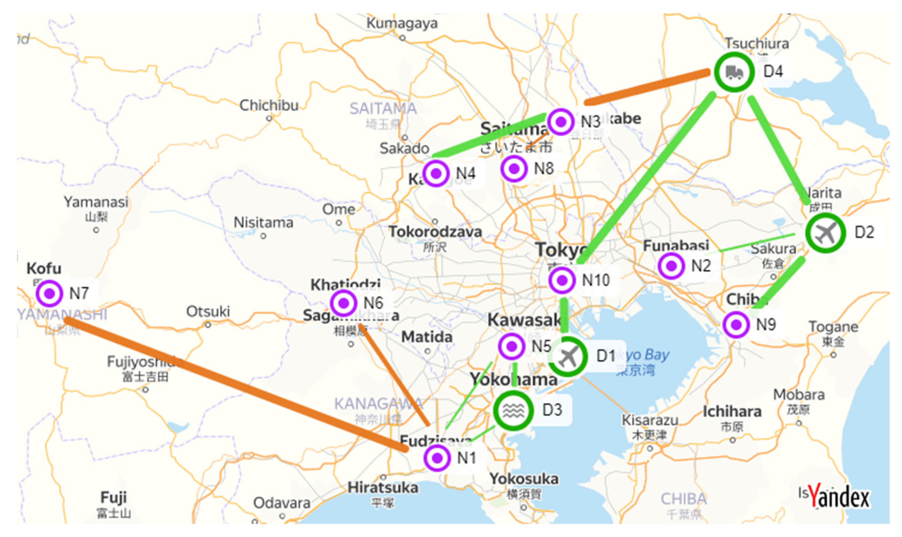
Figure 3 shows a map with all the arcs involved in the optimal routes. In the figure, we can see that the proposed routes are reliable, in the sense of more than 50% probability rate for a successfully executed humanitarian operation. As shown in Table 8, the minimum probability of traversing an arc is 0.52, and the global reliability of the solution is 2.5%, which is an acceptable value considering that the reliability is calculated as a product of the probability of all arcs used in the solution. The total cost is US$995,107, which is only 4893 below the budget limit of 1,000,000. This solution fully satisfies the priorities for nodes N7 and N10, set for meeting the total demand of N7 by 100% (priority = 1) and total demand of N10 by 80% (priority = 0.8).
Table 12 shows changes in load flow over the time horizon. Based on changes in the load flow, we can analyze which nodes were used as transshipment facilities. In Table 12, we can see that nodes N1, N3 and N5 in some time periods have a positive increase in the amount of load, followed by a negative. This indicates that aid was delivered to the node by one group of vehicles, intended for distribution to other nodes by another group of vehicles. Consequently, the nodes were used as transshipment points.
Table 13 shows the number of vehicles starting to travel from node i to node j at a period of time t. As we can see from the schedule, the distribution schedule includes 267 vehicles, which is higher than the total number of available vehicles of 244 (119 small, 81 medium, and 44 large). This is due to the fact that some vehicles perform multiple trips. Analyzing the solution further, we can see that node D4 only uses 9 of its 50 available small vehicles. The number of vehicles leaving the depots appears to be 222, but since 19 of them have been reused, the total number of vehicles used in this solution is in fact 203. It can also be noted that the last time period in which a shipment was performed is period 20, and the full distribution was completed after two more time periods, corresponding to 1.83 h after the start of the operation. It is assumed that a vehicle may leave the node i with the loaded aid or the vehicle may be requested from a nearby node j in order to pick up the aid from that node. In the latter case, the vehicle will leave node i empty. The presented distribution schedule shown in Table 13 does not state whether a vehicle is loaded or empty, and therefore, in Table 14, the schedule of aid distribution in the time periods is presented. This schedule does not reflect the amount of load for each product but only the total quantity to be delivered from node i to node j during time period t. In this case, it is assumed that the products do not require special storage conditions and can be transported simultaneously on the same vehicle. The value 0 in the table represents the situation where a vehicle leaves the node empty to pick up aid from a nearby node for further distribution.
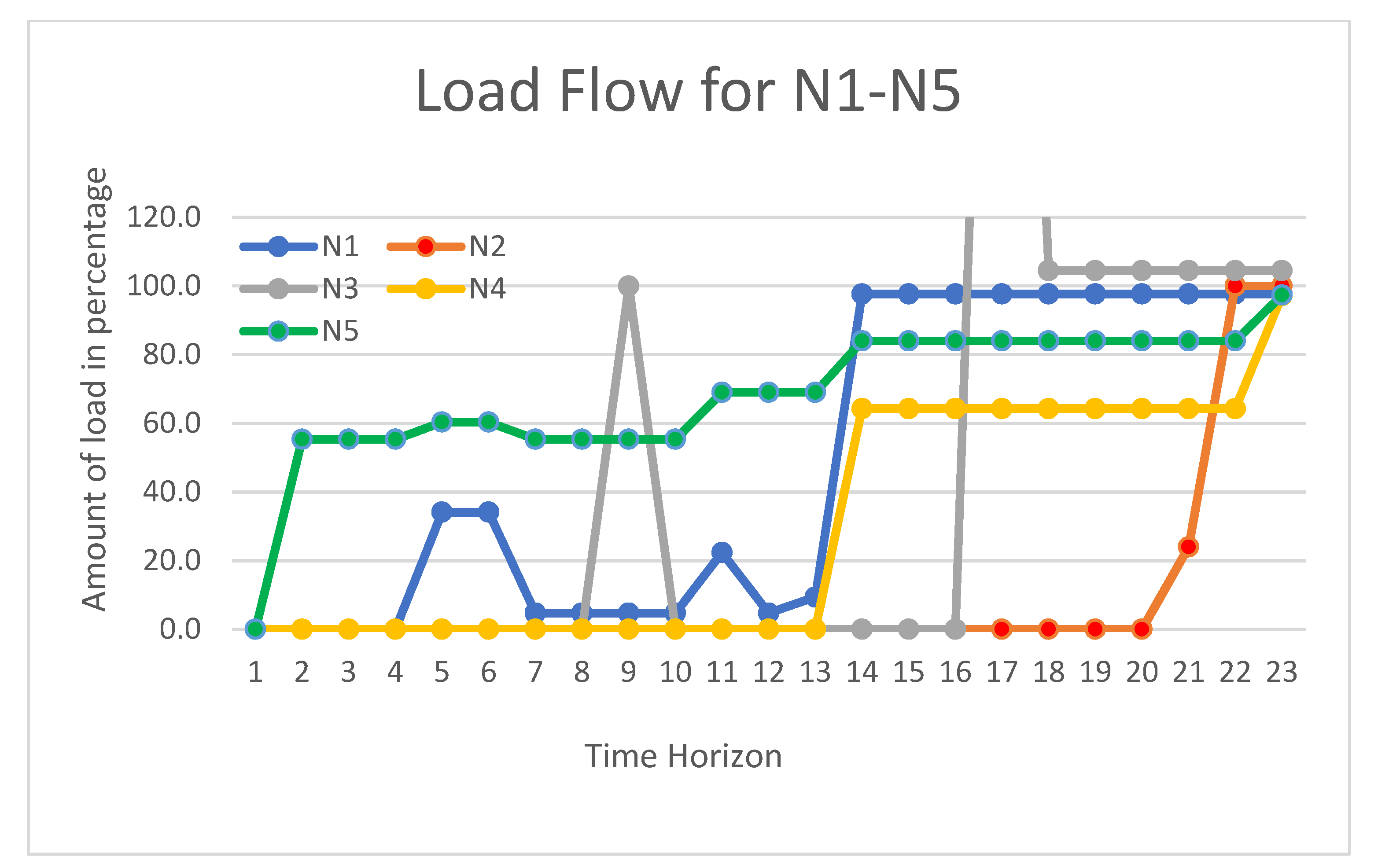
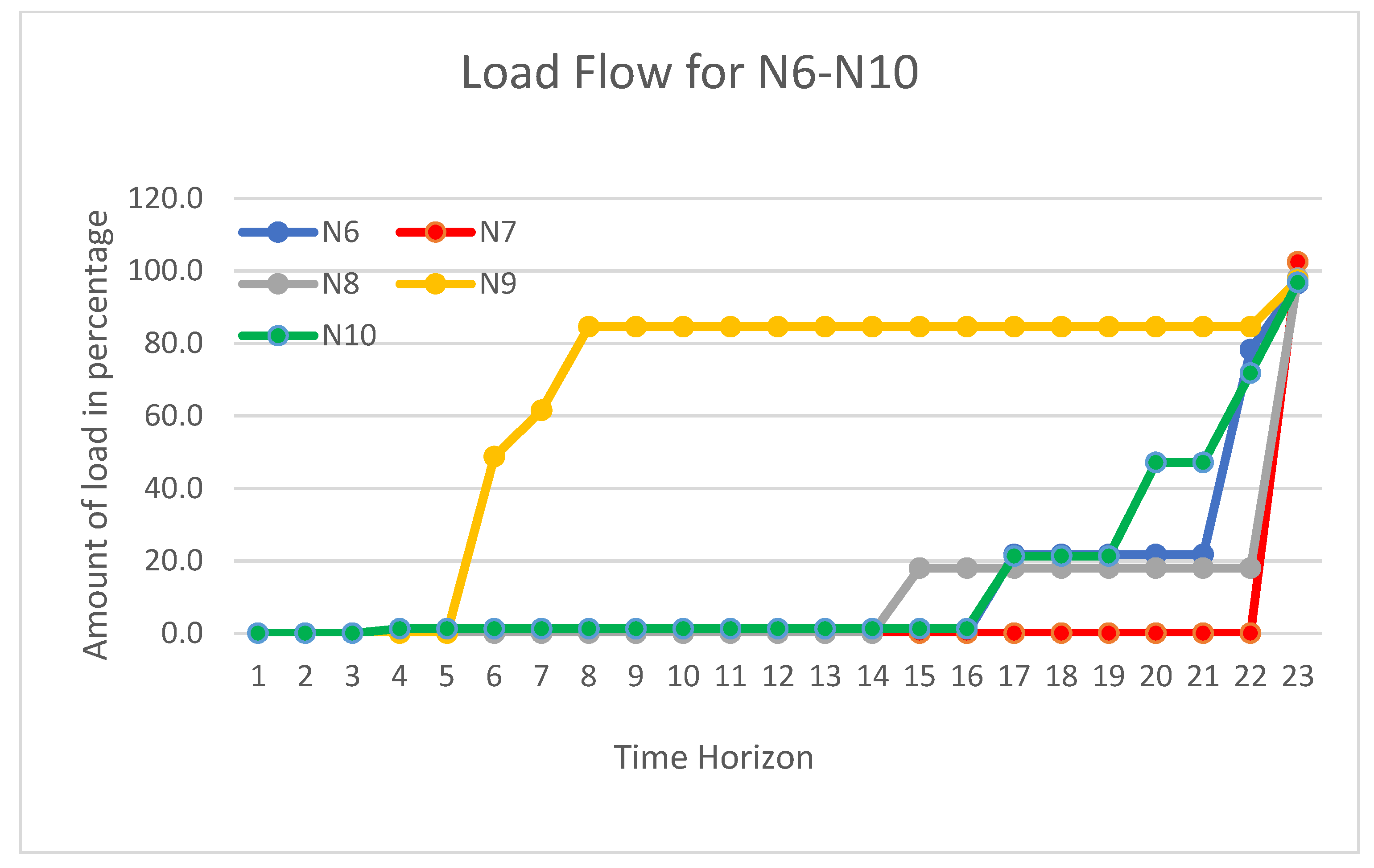
The distribution plan shown in Table 14 is illustrated graphically in Figure 4 for nodes N1–N5 and in Figure 5 for nodes N6–N10. Due to the huge difference in demand of the nodes, the amount received is shown as a percentage of the total demand. Here, we can clearly see when the deliveries are performed and to which degree the demand is met at the different nodes. However, since some nodes are used as transshipment nodes for other demand nodes, the amount received can be reduced from one time period to another if the load was meant for another node. This is particularly evident for node N3, which has four times the demand in place in period 17 before it is transshipped further to the final destination in N8.
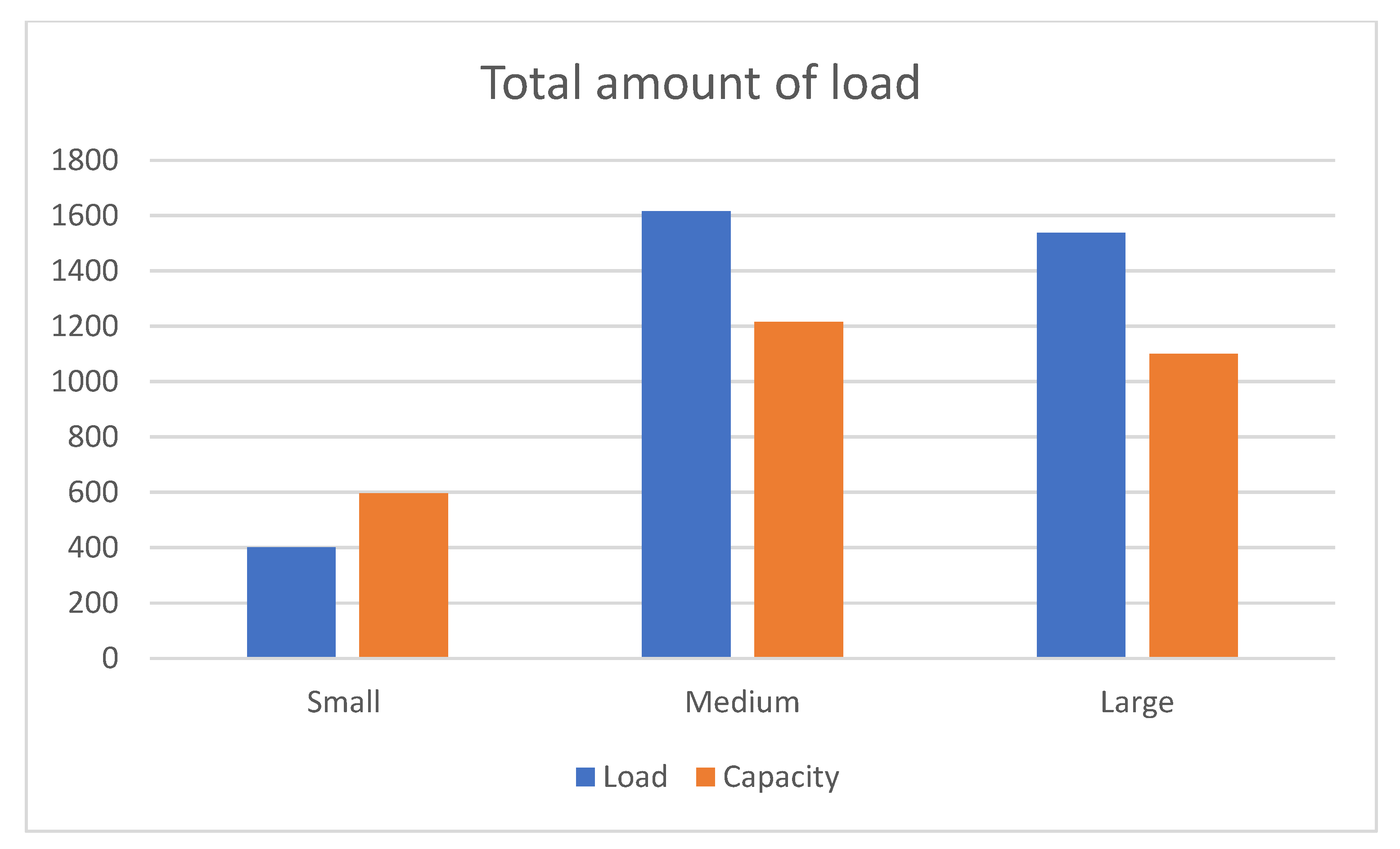
It is also interesting to see the amount of load distributed by the different vehicle types. Figure 6 shows the load transported compared to the total capacity of the vehicle types found by multiplying the number of available vehicles by the capacity of the vehicle type. Here, we can see that the small vehicles are not utilized in full, mainly since node D4 only uses a small fraction of the vehicles available of that type. For the medium and large vehicles, however, the load exceeds the capacity, meaning that some vehicles are used several times. It is clear from the costs and conditions given in this test case that larger vehicles should be preferred to smaller when this is possible.
6. Conclusions
We have presented an extended lexicographical dynamic flow model for solving the multi-commodity aid distribution problem in case of disasters. The model is based on multi-objective optimization in two steps, where the main priority is to maximize the amount of aid to deliver, while other objectives are considered using a goal-programming approach. For testing the model, a case study was performed on a recent typhoon disaster in Japan. The model was used to solve the problem of making a distribution plan of aid from distribution centers to ten demand nodes located in different regional centers in the disastrous area. The plan showed how a maximum amount of aid could be distributed within short time considering other aspects such as costs, reliability, equity, and different priorities.
The main contribution of this research is the extended model in combination with the new case study with realistic data. A future direction of research could be to include even more realistic aspects in the model and to incorporate such a model in a decision aid system to be used when natural disasters appear.
Author Contributions
Conceptualization, investigation, methodology, and software: D.H.; Formal analysis: D.H., U.P., and A.H.; writing—original draft preparation, visualization, D.H. and U.P.; writing—review and editing, D.H., U.P., and A.H.; Supervision: A.H. All authors have read and agreed to the published version of the manuscript.
Funding
This research received no external funding.
Institutional Review Board Statement
Not applicable.
Informed Consent Statement
Not applicable.
Data Availability Statement
Data used in the study is available through public sources as stated in the article.
Conflicts of Interest
The authors declare no conflict of interest.
Appendix A

Table A1.
Network characteristics.
| From | To | Length (km) | Speed (km/h) | Arc Reliability |
|---|---|---|---|---|
| D1 | D3 | 25 | 90 | 0.88 |
| D1 | N2 | 35 | 90 | 0.85 |
| D1 | N5 | 4 | 50 | 0.78 |
| D1 | N9 | 50 | 90 | 0.89 |
| D1 | N10 | 20 | 90 | 0.97 |
| D2 | D4 | 51 | 90 | 0.79 |
| D2 | N2 | 45 | 50 | 0.99 |
| D2 | N9 | 35 | 90 | 0.8 |
| D3 | D1 | 25 | 90 | 0.88 |
| D3 | N1 | 26 | 50 | 0.99 |
| D3 | N5 | 20 | 70 | 0.98 |
| D3 | N6 | 50 | 70 | 0.29 |
| D4 | D2 | 51 | 90 | 0.79 |
| D4 | N2 | 67 | 90 | 0.1 |
| D4 | N3 | 52 | 90 | 0.52 |
| D4 | N10 | 70 | 90 | 0.87 |
| N1 | D3 | 26 | 50 | 0.99 |
| N1 | N6 | 55 | 70 | 0.59 |
| N1 | N7 | 130 | 90 | 0.61 |
| N1 | N5 | 9 | 50 | 0.99 |
| N2 | D1 | 35 | 90 | 0.85 |
| N2 | D2 | 45 | 50 | 0.99 |
| N2 | D4 | 67 | 90 | 0.1 |
| N2 | N9 | 17 | 50 | 0.89 |
| N2 | N10 | 22 | 70 | 0.99 |
| N3 | D4 | 52 | 90 | 0.52 |
| N3 | N4 | 40 | 90 | 0.97 |
| N3 | N8 | 20 | 50 | 0.56 |
| N3 | N10 | 50 | 70 | 0.24 |
| N4 | N3 | 40 | 90 | 0.97 |
| N4 | N7 | 150 | 90 | 0.79 |
| N4 | N8 | 20 | 50 | 0.89 |
| N4 | N10 | 50 | 70 | 0.21 |
| N5 | D1 | 4 | 50 | 0.78 |
| N5 | D3 | 20 | 70 | 0.98 |
| N5 | N1 | 9 | 50 | 0.99 |
| N5 | N10 | 19 | 90 | 0.79 |
| N6 | D3 | 50 | 70 | 0.29 |
| N6 | N1 | 55 | 70 | 0.59 |
| N6 | N7 | 98 | 90 | 0.88 |
| N6 | N10 | 50 | 70 | 0.53 |
| N7 | N1 | 130 | 90 | 0.61 |
| N7 | N4 | 150 | 90 | 0.79 |
| N7 | N6 | 98 | 90 | 0.88 |
| N8 | N3 | 20 | 50 | 0.56 |
| N8 | N4 | 20 | 50 | 0.9 |
| N8 | N10 | 30 | 90 | 0.2 |
| N9 | D1 | 50 | 90 | 0.89 |
| N9 | D2 | 35 | 90 | 0.8 |
| N9 | N2 | 17 | 50 | 0.89 |
| N10 | D1 | 20 | 90 | 0.97 |
| N10 | D4 | 70 | 90 | 0.87 |
| N10 | N2 | 22 | 70 | 0.99 |
| N10 | N3 | 50 | 70 | 0.24 |
| N10 | N4 | 50 | 70 | 0.21 |
| N10 | N5 | 19 | 90 | 0.79 |
| N10 | N6 | 50 | 70 | 0.53 |
| N10 | N8 | 30 | 90 | 0.2 |
References
- Schumann-Bölsche, D. Logistik in der Katastrophenhilfe. Eurotransport.de, Berlin. 2015. Available online: https://www.eurotransport.de/artikel/gegenseitig-bereichern-logistik-in-der-katastrophenhilfe-6763602.html (accessed on 10 June 2021).
- World Heritage Encyclopedia. Humanitarian Logistics. 2020. Available online: http://worldheritage.org/article/WHEBN0018151097/Humanitarian%20Logistics (accessed on 31 August 2020).
- Ferrer, J.M.; Martín-Campo, F.J.; Ortuño, M.T.; Pedraza-Martínez, A.J.; Tirado, G.; Vitoriano, B. Multi-criteria optimization for last mile distribution of disaster relief aid: Test cases and applications. Eur. J. Oper. Res. 2018, 269, 501–515. [Google Scholar] [CrossRef]
- Guide, D.; Van Wassenhove, L. Dancing with the Devil: Partnering with Industry but Publishing in Academia. Decis. Sci. 2007, 38, 531–546. [Google Scholar] [CrossRef]
- Kunz, N.; Van Wassenhove, L.; Besiou, M.; Hambye, C.; Kovács, G. Relevance of humanitarian logistics research: Best practices and way forward. Int. J. Oper. Prod. Manag. 2017, 37, 1585–1599. [Google Scholar] [CrossRef]
- Carroll, A.; Neu, J. Volatility, unpredictability and asymmetry: An organising framework for humanitarian Logistics operations? Manag. Res. News 2009, 32, 1024–1037. [Google Scholar] [CrossRef]
- Overstreet, R.E.; Hall, D.L.; Hanna, J.B.; Rainer, R.K. Research in humanitarian logistics. J. Humanit. Logist. Supply Chain Manag. 2011, 1, 114–131. [Google Scholar] [CrossRef]
- Anuar, W.K.; Lee, L.S.; Pickl, S.; Seow, H.-V. Vehicle routing optimization in humanitarian operations: A survey on modelling and optimization approaches. Appl. Sci. 2021, 11, 667. [Google Scholar] [CrossRef]
- UCM-HUMLOG. Decision Aid Models for Logistics and Disaster Management (Humanitarian Logistics) Resource Group 2020; Complutense University of Madrid: Madrid, Spain, 2020; Available online: http://blogs.mat.ucm.es/humlog/ (accessed on 10 June 2021).
- Vitoriano, B.; Rodríguez, J.T.; Tirado, G.; Martín-Campo, F.J.; Ortuño, M.T.; Montero, J. Intelligent decision-making models for disaster management. Hum. Ecol. Risk Assess. 2015, 21, 1341–1360. [Google Scholar] [CrossRef]
- Mejia-Argueta, C.; Gaytán, J.; Caballero, R.; Molina, J.; Vitoriano, B. Multicriteria optimization approach to deploy humanitarian logistics operations integrally during floods. Int. Trans. Oper. Res. 2018, 25, 1053–1079. [Google Scholar] [CrossRef] [Green Version]
- Vitoriano, B.; Ortuño, T.; Tirado, G. HADS, a goal-programming-based humanitarian aid distribution system. J. Multi-Criteria Decis. Anal. 2009, 16, 55–64. [Google Scholar] [CrossRef]
- Flores, I.; Ortuño, M.T.; Tirado, G. Supported evacuation for disaster relief through lexicographic goal programming. Mathematics 2020, 8, 648. [Google Scholar] [CrossRef]
- Rennemo, S.J.; Rø, K.F.; Hvattum, L.M.; Tirado, G. A three-stage stochastic facility routing model for disaster response planning. Transp. Res. Part E 2014, 62, 116–135. [Google Scholar] [CrossRef] [Green Version]
- Monzón, J.; Liberatore, F.; Vitoriano, B. A mathematical pre-disaster model with uncertainty and multiple criteria for facility location and network fortification. Mathematics 2020, 8, 529. [Google Scholar] [CrossRef] [Green Version]
- Ferrer, J.M.; Ortuño, M.T.; Tirado, G. A GRASP metaheuristic for humanitarian aid distribution. J. Heuristics 2016, 22, 55–87. [Google Scholar] [CrossRef]
- Ferrer, J.M.; Ortuño, M.T.; Tirado, G. A new ant-colony-based methodology for disaster relief. Mathematics 2020, 8, 518. [Google Scholar] [CrossRef] [Green Version]
- Liberatore, F.; Ortuño, M.T.; Tirado, G.; Vitoriano, B.; Scaparra, M.P. A hierarchical compromise model for the joint optimization of recovery operations and distribution of emergency goods in Humanitarian Logistics. Comput. Oper. Res. 2014, 42, 3–13. [Google Scholar] [CrossRef]
- Tirado, G.; Martín-Campo, F.J.; Vitoriano, B.; Ortuño, M.T. A lexicographical dynamic flow model for relief operations. Int. J. Comput. Intell. Syst. 2014, 7, 45–57. [Google Scholar] [CrossRef] [Green Version]
- Ortuño, M.T.; Tirado, G.; Vitoriano, B. A lexicographical goal programming-based decision support system for logistics of Humanitarian Aid. TOP 2011, 19, 464–479. [Google Scholar] [CrossRef]
- Feo, T.A.; Resende, M.G.C. A probabilistic heuristic for a computationally difficult set covering problem. Oper. Res. Lett. 1989, 8, 67–71. [Google Scholar] [CrossRef]
- Vitoriano, B.; Ortuño, M.T.; Tirado, G.; Montero, J. A multi-criteria optimization model for humanitarian aid distribution. J. Glob. Optim. 2011, 51, 189–208. [Google Scholar] [CrossRef]
- Jones, D.F.; Tamiz, M. Goal programming in the period 1990–2000. In Multiple Criteria Optimization State of the Art Annotated Bibliographic Surveys; Ehrgott, M., Gandibleux, X., Eds.; Kluwer Academic Publishers: Boston, MA, USA, 2002. [Google Scholar]
- Romero, C. Handbook of Critical Issues in Goal Programming; Pergamon Press: Oxford, UK, 1991. [Google Scholar]
- Pedraza-Martinez, A.J.; Wassenhove, L.N.V. Empirically grounded research in humanitarian operations management: The way forward. Oper. Manag. 2016, 45, 1–10. [Google Scholar] [CrossRef]
- Japan Meteorological Agency. Tropical Cyclone Information 2020. Available online: https://www.jma.go.jp/en/typh/ (accessed on 10 June 2021).
- Reliefweb. Japan Tropical Cyclone Hagibis. European Commission’s Directorate-General for European Civil Protection and Humanitarian Aid Operations 2020. Available online: https://reliefweb.int/map/japan/japan-tropical-cyclone-hagibis-dg-echo-daily-map-14102019 (accessed on 10 June 2021).
- SBJ. Statistics Bureau of Japan 2020. Available online: http://www.stat.go.jp/english/index.html (accessed on 10 June 2021).
- Statistics Japan. Prefecture Comparisons 2020. Available online: https://stats-japan.com/t/categ/50004 (accessed on 10 June 2021).
- OCHA. Japan Humanitarian Data Exchange. The United Nations Office for the Coordination of Humanitarian Affairs (OCHA), 2020. Available online: https://data.humdata.org/group/jpn (accessed on 10 June 2021).
- Japan Platform. Emergency Humanitarian Aid Organization—NGO Japan Platform 2020. Available online: https://www.japanplatform.org/E/ (accessed on 10 June 2021).
- MLIT. Ministry of Land, Infrastructure, Transport and Tourism of Japan 2020. Available online: https://www.mlit.go.jp/en/index.html (accessed on 10 June 2021).
- UNOCHA. World Humanitarian Data and Trends. United Nations Office for the Coordination of Humanitarian Affairs, 2020. Available online: https://www.unocha.org/ (accessed on 10 June 2021).
- EM-DAT. The International Disaster Database. Centre for Research on the Epidemiology of Disasters, 2020. Available online: https://www.emdat.be/database (accessed on 10 June 2021).
Figure 1.
The path of typhoon Hagibis over time [26].
Figure 1.
The path of typhoon Hagibis over time [26].

Figure 2.
Transport network for the operation (https://yandex.com/maps/-/CCQ2F8edtD, accessed on 10 June 2021).
Figure 2.
Transport network for the operation (https://yandex.com/maps/-/CCQ2F8edtD, accessed on 10 June 2021).

Figure 3.
Humanitarian aid distribution network for the optimal solution.

Figure 4.
Load flow for nodes N1–N5.

Figure 5.
Load flow for nodes N6–N10.

Figure 6.
Amount of load distributed with different vehicle types.

Table 1.
Sets and indices.
| : | Set of demand nodes and depots | |
| : | Set of arcs represents existing links between nodes | |
| : | Planned time horizon to complete the operation | |
| : | Set of vehicles, defined by types | |
| : | Set of products | |
| : | Set of goals/objectives | |
| : | ||
| : | ||
| : | ||
| : | , respectively | |
| . | : | |
| : |
Table 2.
Parameters.
| : | Demand of product at node in tons | |
| : | Available supply of product at node in tons | |
| : | Length of arc in km | |
| : | Maximum velocity on arc in km per hour | |
| : | Probability of crossing the arc | |
| : | Capacity of vehicle type in tons | |
| : | Maximum velocity of vehicle type in km per hour | |
| : | Number of available vehicles of type at node | |
| : | Total number of vehicle types available for the operation | |
| : | Travel time of arc using vehicle of type | |
| : | Empty travel cost, i.e., fixed cost of using arc with vehicle of type per km | |
| : | Load travel cost, i.e., variable cost of using arc with vehicle of type , per km, and ton of product | |
| : | Priority level of node | |
| : | Target for criterion ; defined by decision maker | |
| : | Weight of criterion defined by decision maker | |
| : | Time measure helping adjust the length of time period | |
| : | Large value to create bounds for some constraints | |
| : | Fixed deviation of delivered aid, in tons | |
| : | Total amount of product desired to be distributed in the operation, in tons | |
| : | Budget available to perform the operation |
Table 3.
Variables.
| : | Load of product carried from to using vehicle of type and starting in period , in tons | |
| : | Load of product stored at node at the beginning of period in tons | |
| : | Number of vehicles of type that start traveling from to in period | |
| : | Number of vehicles of type available at node at the beginning of period | |
| : | Binary variable taking value 1 if a vehicle of type uses arc , 0 otherwise | |
| : | Binary variable taking value 1 if any vehicle uses arc , 0 otherwise | |
| : | Binary variable taking value 1 if load has been delivered in period , 0 otherwise | |
| : | Variable showing unwanted deviation of the criterion from its target, in units of criterion | |
| : | Variable showing unwanted deviation from desired amount of delivered aid, in tons |
Table 4.
Considered criteria.
| : | Total cost of the operation, in US dollars. | |
| : | Number of time periods required to complete the operation. | |
| : | Time penalties variable adding higher penalties to long operations. | |
| : | Criterion of equity of food distribution. 0 if food demand of all nodes is completely fulfilled and positive otherwise. | |
| : | Criterion of equity of medicine distribution. 0 if medicine demand of all nodes is completely fulfilled and positive otherwise. | |
| : | Demand satisfaction priority criterion in the specific nodes. 0 if demand of priority nodes is completely fulfilled and positive otherwise. | |
| : | Reliability criterion indicates the most unreliable arc used in the operation. | |
| : | Global route reliability criterion shows reliability of the whole set of arcs used in the operation. |
Table 5.
Characteristics of the humanitarian operation.
| Name | Nodes | Demand (Tons) | Supply (Tons) | Availability of Vehicles of Each Type | Priority | ||||
|---|---|---|---|---|---|---|---|---|---|
| Food | Medicine | Food | Medicine | Small | Medium | Large | |||
| Haneda Airport | D1 | 1100 | 200 | 50 | 30 | 20 | |||
| Narita Airport | D2 | 440 | 80 | 12 | 8 | 2 | |||
| Yokohama Port | D3 | 230 | 80 | 7 | 13 | 2 | |||
| Tsuchiura DC | D4 | 1270 | 0 | 50 | 30 | 20 | |||
| Fujisawa | N1 | 75 | 10 | ||||||
| Funabashi | N2 | 105 | 20 | ||||||
| Kasukabe | N3 | 40 | 5 | ||||||
| Kawagoe | N4 | 60 | 10 | ||||||
| Kawasaki | N5 | 255 | 45 | ||||||
| Hachioji | N6 | 95 | 20 | ||||||
| Kofu | N7 | 35 | 5 | 1 | |||||
| Saitama | N8 | 225 | 25 | ||||||
| Chiba | N9 | 165 | 30 | ||||||
| Tokyo | N10 | 1530 | 270 | 0.8 | |||||
Table 6.
Characteristics and operational costs of the vehicle.
| Vehicle Types | Vehicle Capacity (tons) | Speed (km/h) | Fixed Cost (US$/km) | Variable Cost (US$/(km·Ton·Product)) | |
|---|---|---|---|---|---|
| Food | Medicine | ||||
| small | 5 | 100 | 20 | 1 | 1 |
| medium | 15 | 90 | 50 | 1.1 | 1 |
| large | 25 | 80 | 70 | 1.3 | 1 |
Table 7.
Pay-off matrix.
| Criterion | Cost, $ | Time, Hour | TP | EqF | EqM | Prio | Rel | GR | |
|---|---|---|---|---|---|---|---|---|---|
| log | % | ||||||||
| Cost | 799,342 | 2.5 | 5525 | 1 | 1 | 1.8 | 0.52 | −2.4 | 9.4 |
| Operation Time | 998,942 | 1.7 | 1240 | 1 | 1 | 1.79 | 0.1 | −6.9 | 0.11 |
| Time Penalty | 974,028 | 0.7 | 14 | 1 | 1 | 1.8 | 0.52 | −1.9 | 13.8 |
| Equity Food | 999,112 | 2.5 | 5525 | 0 | 1 | 0.25 | 0.1 | −7.2 | 0.07 |
| Equity Medicine | 997,901 | 2.5 | 5525 | 1 | 0.2 | 1.49 | 0.29 | −4.7 | 0.84 |
| Priority | 991,038 | 2.5 | 5525 | 1 | 1 | 0 | 0.29 | −3.7 | 2.5 |
| Reliability | 998,680 | 2.5 | 5525 | 1 | 1 | 0.82 | 0.87 | −0.37 | 69.3 |
| Global Route Rel. | 997,824 | 2.5 | 5525 | 1 | 1 | 0.76 | 0.87 | −0.21 | 81.1 |
Table 8.
Solution result for aggregated goals.
| Criteria | Cost, $ | Time, Hour | TP | EqF | EqM | Prio | Rel | GR | |
|---|---|---|---|---|---|---|---|---|---|
| log | % | ||||||||
| Cost and Time and TP | 799,802 | 1.7 | 14 | 1 | 1 | 1.76 | 0.52 | −1.61 | 19.8 |
| Cost and Rel and GR | 987,939 | 2.5 | 5525 | 1 | 1 | 0.74 | 0.87 | −0.21 | 81.1 |
| Cost and EqF and EqM and Prio | 936,175 | 2.5 | 5525 | 0.002 | 0.2 | 0 | 0.1 | −8.5 | 0.02 |
| Cost and Time and TP and EqF and EqM | 993,456 | 1.8 | 1785 | 0 | 0.2 | 0.024 | 0.1 | −10.1 | 0.001 |
| EqF and EqM and Prio | 999,967 | 2.5 | 5525 | 0.002 | 0.2 | 0 | 0.1 | −11.4 | 0.001 |
| Rel and GR | 999,973 | 6 | 5525 | 1 | 1 | 0.74 | 0.87 | −0.21 | 81.1 |
| Optimal solution | 995,107 | 1.8 | 1785 | 0 | 0.2 | 0 | 0.52 | −3.7 | 2.5 |
Table 9.
Distribution plan of food for each set of criteria.
| Node | N1 | N2 | N3 | N4 | N5 | N6 | N7 | N8 | N9 | N10 |
|---|---|---|---|---|---|---|---|---|---|---|
| Demand, tons | 75 | 105 | 40 | 60 | 255 | 95 | 35 | 225 | 165 | 1530 |
| Criteria | Demand satisfaction, % | |||||||||
| Cost | 140 | 66 | 2037 | 0 | 480 | 0 | 0 | 0 | 224 | 0 |
| Operation Time | 286 | 804 | 487 | 0 | 372 | 0 | 0 | 0 | 212 | 1 |
| Time Penalty | 0 | 0 | 2762 | 0 | 521 | 0 | 0 | 0 | 90 | 0 |
| Equity Food | 100 | 100 | 100 | 100 | 100 | 100 | 100 | 100 | 100 | 100 |
| Equity Medicine | 0 | 57 | 1412 | 0 | 413 | 0 | 0 | 0 | 396 | 16 |
| Priority | 224 | 671 | 2062 | 0 | 329 | 0 | 134 | 0 | 0 | 0 |
| Reliability | 0 | 123 | 0 | 0 | 90 | 0 | 0 | 0 | 133 | 131 |
| Global Route Rel | 266 | 176 | 0 | 0 | 0 | 0 | 0 | 0 | 0 | 143 |
| Aggregated criteria | Demand satisfaction, % | |||||||||
| Cost and Time and TP | 666 | 414 | 2925 | 0 | 98 | 0 | 0 | 0 | 90 | 5 |
| Cost and Rel and GR | 266 | 190 | 0 | 0 | 0 | 0 | 0 | 0 | 0 | 142 |
| Cost and EqF and EqM and Prio | 100 | 100 | 100 | 100 | 101 | 100 | 100 | 100 | 100 | 99 |
| Cost and Time and TP and EqF and EqM | 100 | 100 | 100 | 100 | 100 | 100 | 100 | 100 | 100 | 100 |
| EqF and EqM and Prio | 100 | 100 | 100 | 100 | 101 | 100 | 100 | 100 | 100 | 99 |
| Rel and GR | 253 | 190 | 0 | 0 | 0 | 0 | 0 | 0 | 0 | 143 |
Table 10.
Distribution plan of medicine for each set of criteria.
| Nodes | N1 | N2 | N3 | N4 | N5 | N6 | N7 | N8 | N9 | N10 |
|---|---|---|---|---|---|---|---|---|---|---|
| Demand, tons | 10 | 20 | 5 | 10 | 45 | 20 | 5 | 25 | 30 | 270 |
| Criteria | Demand satisfaction, % | |||||||||
| Cost | 0 | 25 | 0 | 0 | 622 | 0 | 0 | 0 | 250 | 0 |
| Operation Time | 800 | 400 | 0 | 0 | 56 | 0 | 0 | 0 | 583 | 0 |
| Time Penalty | 800 | 1000 | 0 | 0 | 0 | 0 | 0 | 0 | 267 | 0 |
| Equity Food | 0 | 0 | 0 | 0 | 622 | 0 | 0 | 0 | 267 | 0 |
| Equity Medicine | 100 | 80 | 80 | 80 | 80 | 105 | 80 | 80 | 80 | 80 |
| Priority | 0 | 275 | 0 | 0 | 567 | 0 | 500 | 0 | 83 | 0 |
| Reliability | 0 | 400 | 0 | 0 | 178 | 0 | 0 | 0 | 0 | 74 |
| Global Route Rel | 800 | 650 | 0 | 0 | 0 | 0 | 0 | 0 | 0 | 56 |
| Aggregated criteria | Demand satisfaction, % | |||||||||
| Cost and Time and TP | 300 | 0 | 0 | 0 | 556 | 0 | 0 | 0 | 267 | 0 |
| Cost and Rel and GR | 800 | 400 | 0 | 0 | 0 | 0 | 0 | 0 | 0 | 74 |
| Cost and EqF and EqM and Prio | 80 | 80 | 80 | 80 | 87 | 95 | 120 | 80 | 80 | 80 |
| Cost and Time and TP and EqF and EqM | 80 | 100 | 80 | 90 | 80 | 80 | 100 | 84 | 83 | 80 |
| EqF and EqM and Prio | 80 | 80 | 80 | 80 | 91 | 80 | 120 | 80 | 83 | 80 |
| Rel and GR | 800 | 400 | 0 | 0 | 0 | 0 | 0 | 0 | 0 | 74 |
Table 11.
Optimal solution: distribution plan for demand nodes.
| Node | Demand, tons | Satisfaction, % | Completion Time, Hours | ||
|---|---|---|---|---|---|
| Food | Medicine | Food | Medicine | ||
| N1 | 75 | 10 | 100 | 80 | 1.08 |
| N2 | 105 | 20 | 100 | 100 | 1.75 |
| N3 | 40 | 5 | 107 | 80 | 1.42 |
| N4 | 60 | 10 | 100 | 80 | 1.83 |
| N5 | 255 | 45 | 100 | 82 | 1.83 |
| N6 | 95 | 20 | 100 | 80 | 1.83 |
| N7 | 35 | 5 | 100 | 120 | 1.83 |
| N8 | 225 | 25 | 100 | 80 | 1.83 |
| N9 | 165 | 30 | 100 | 83 | 1.83 |
| N10 | 1530 | 270 | 99 | 80 | 1.83 |
Table 12.
Load flow over time horizon.
| Period | Hours Elapsed | D1 | D2 | D3 | D4 | N1 | N2 | N3 | N4 | N5 | N6 | N7 | N8 | N9 | N10 |
|---|---|---|---|---|---|---|---|---|---|---|---|---|---|---|---|
| 0 | 0.00 | 1300 | 520 | 310 | 1270 | 0 | 0 | 0 | 0 | 0 | 0 | 0 | 0 | 0 | 0 |
| 1 | 0.08 | 1041 | 375 | 295 | 1225 | 0 | 0 | 0 | 0 | 0 | 0 | 0 | 0 | 0 | 0 |
| 2 | 0.17 | 1041 | 370 | 295 | 1180 | 0 | 0 | 0 | 0 | 166 | 0 | 0 | 0 | 0 | 0 |
| 3 | 0.25 | 1041 | 320 | 295 | 1180 | 0 | 0 | 0 | 0 | 166 | 0 | 0 | 0 | 0 | 0 |
| 4 | 0.33 | 1041 | 320 | 280 | 1180 | 0 | 0 | 0 | 0 | 166 | 0 | 0 | 0 | 0 | 23 |
| 5 | 0.42 | 1041 | 320 | 230 | 1180 | 29 | 0 | 0 | 0 | 181 | 0 | 0 | 0 | 0 | 23 |
| 6 | 0.50 | 1041 | 320 | 205 | 1180 | 29 | 0 | 0 | 0 | 181 | 0 | 0 | 0 | 95 | 23 |
| 7 | 0.58 | 1041 | 320 | 85 | 820 | 4 | 0 | 0 | 0 | 166 | 0 | 0 | 0 | 120 | 23 |
| 8 | 0.67 | 1056 | 320 | 85 | 820 | 4 | 0 | 0 | 0 | 166 | 0 | 0 | 0 | 165 | 23 |
| 9 | 0.75 | 1056 | 320 | 85 | 650 | 4 | 0 | 45 | 0 | 166 | 0 | 0 | 0 | 165 | 23 |
| 10 | 0.83 | 1056 | 290 | 40 | 630 | 4 | 0 | 0 | 0 | 166 | 0 | 0 | 0 | 165 | 23 |
| 11 | 0.92 | 1056 | 195 | 40 | 385 | 19 | 0 | 0 | 0 | 207 | 0 | 0 | 0 | 165 | 23 |
| 12 | 1.00 | 1060 | 195 | 40 | 285 | 4 | 0 | 0 | 0 | 207 | 0 | 0 | 0 | 165 | 23 |
| 13 | 1.08 | 1060 | 195 | 40 | 285 | 8 | 0 | 0 | 0 | 207 | 0 | 0 | 0 | 165 | 23 |
| 14 | 1.17 | 1060 | 195 | 40 | 285 | 83 | 0 | 0 | 45 | 252 | 0 | 0 | 0 | 165 | 23 |
| 15 | 1.25 | 1060 | 195 | 40 | 285 | 83 | 0 | 0 | 45 | 252 | 0 | 0 | 45 | 165 | 23 |
| 16 | 1.33 | 1060 | 195 | 40 | 285 | 83 | 0 | 0 | 45 | 252 | 0 | 0 | 45 | 165 | 23 |
| 17 | 1.42 | 595 | 170 | 40 | 285 | 83 | 0 | 177 | 45 | 252 | 25 | 0 | 45 | 165 | 383 |
| 18 | 1.50 | 595 | 170 | 40 | 285 | 83 | 0 | 47 | 45 | 252 | 25 | 0 | 45 | 165 | 383 |
| 19 | 1.58 | 350 | 170 | 0 | 285 | 83 | 0 | 47 | 45 | 252 | 25 | 0 | 45 | 165 | 383 |
| 20 | 1.67 | 0 | 170 | 0 | 285 | 83 | 0 | 47 | 45 | 252 | 25 | 0 | 45 | 165 | 848 |
| 21 | 1.75 | 0 | 170 | 0 | 285 | 83 | 30 | 47 | 45 | 252 | 25 | 0 | 45 | 165 | 848 |
| 22 | 1.83 | 0 | 170 | 0 | 285 | 83 | 125 | 47 | 45 | 252 | 90 | 0 | 45 | 165 | 1293 |
| 23 | 1.92 | 0 | 170 | 0 | 285 | 83 | 125 | 47 | 68 | 292 | 111 | 41 | 245 | 190 | 1743 |
Table 13.
Distribution schedule for the operation: number of vehicles.
| From | To | Vehicle Type | Time Period | |||||||||||||||||||
|---|---|---|---|---|---|---|---|---|---|---|---|---|---|---|---|---|---|---|---|---|---|---|
| 1 | 2 | 3 | 4 | 5 | 6 | 7 | 8 | 9 | 10 | 11 | 12 | 13 | 14 | 15 | 16 | 17 | 18 | 19 | 20 | |||
| D1 | N5 | small | 25 | |||||||||||||||||||
| medium | 3 | |||||||||||||||||||||
| large | 3 | |||||||||||||||||||||
| N10 | small | 25 | ||||||||||||||||||||
| medium | 31 | 3 | ||||||||||||||||||||
| large | 1 | 8 | 9 | |||||||||||||||||||
| D2 | D4 | small | 1 | 1 | ||||||||||||||||||
| medium | ||||||||||||||||||||||
| large | 1 | |||||||||||||||||||||
| N2 | small | 1 | ||||||||||||||||||||
| medium | 2 | 6 | ||||||||||||||||||||
| large | ||||||||||||||||||||||
| N9 | small | 1 | 9 | |||||||||||||||||||
| medium | 6 | |||||||||||||||||||||
| large | 1 | 1 | ||||||||||||||||||||
| D3 | N1 | small | ||||||||||||||||||||
| medium | 1 | 5 | ||||||||||||||||||||
| large | 2 | 1 | ||||||||||||||||||||
| N5 | small | 8 | ||||||||||||||||||||
| medium | 1 | 3 | 3 | |||||||||||||||||||
| large | ||||||||||||||||||||||
| D4 | N3 | small | 9 | |||||||||||||||||||
| medium | 3 | 3 | ||||||||||||||||||||
| large | 8 | 1 | ||||||||||||||||||||
| N10 | small | |||||||||||||||||||||
| medium | 24 | |||||||||||||||||||||
| large | 8 | 4 | ||||||||||||||||||||
| N1 | N6 | small | ||||||||||||||||||||
| medium | 1 | |||||||||||||||||||||
| large | 1 | 2 | 1 | |||||||||||||||||||
| N7 | small | |||||||||||||||||||||
| medium | 3 | |||||||||||||||||||||
| large | ||||||||||||||||||||||
| N3 | N4 | small | ||||||||||||||||||||
| medium | 3 | |||||||||||||||||||||
| large | 1 | |||||||||||||||||||||
| N8 | small | |||||||||||||||||||||
| medium | 3 | |||||||||||||||||||||
| large | 8 | |||||||||||||||||||||
| N5 | D1 | small | ||||||||||||||||||||
| medium | 1 | 3 | 3 | |||||||||||||||||||
| large | 1 | |||||||||||||||||||||
| D3 | small | 1 | ||||||||||||||||||||
| medium | ||||||||||||||||||||||
| large | 1 | |||||||||||||||||||||
| N1 | small | |||||||||||||||||||||
| medium | 3 | |||||||||||||||||||||
| large | 1 | |||||||||||||||||||||
| N9 | D2 | small | 1 | |||||||||||||||||||
| medium | 6 | |||||||||||||||||||||
| large | 1 | |||||||||||||||||||||
Table 14.
Distribution schedule for the operation: amount of aid.
| From | To | Vehicle Type | Time Period | ||||||||||||||||
|---|---|---|---|---|---|---|---|---|---|---|---|---|---|---|---|---|---|---|---|
| 1 | 2 | 3 | 4 | 5 | 6 | 7 | 8 | 9 | 10 | 11 | 12 | 13 | 17 | 18 | 19 | 20 | |||
| D1 | N5 | small | 125 | ||||||||||||||||
| medium | 45 | ||||||||||||||||||
| large | 66 | ||||||||||||||||||
| N10 | small | 125 | |||||||||||||||||
| medium | 465 | 45 | |||||||||||||||||
| large | 23 | 200 | 225 | ||||||||||||||||
| D2 | D4 | small | 5 | 5 | |||||||||||||||
| medium | |||||||||||||||||||
| large | 25 | ||||||||||||||||||
| N2 | small | 5 | |||||||||||||||||
| medium | 30 | 90 | |||||||||||||||||
| large | |||||||||||||||||||
| N9 | small | 5 | 45 | ||||||||||||||||
| medium | 90 | ||||||||||||||||||
| large | 25 | 25 | |||||||||||||||||
| D3 | N1 | small | |||||||||||||||||
| medium | 15 | 75 | |||||||||||||||||
| large | 50 | 25 | |||||||||||||||||
| N5 | small | 40 | |||||||||||||||||
| medium | 15 | 45 | 45 | ||||||||||||||||
| large | |||||||||||||||||||
| D4 | N3 | small | 45 | ||||||||||||||||
| medium | 45 | 45 | |||||||||||||||||
| large | 200 | 25 | |||||||||||||||||
| N10 | small | ||||||||||||||||||
| medium | 360 | ||||||||||||||||||
| large | 200 | 100 | |||||||||||||||||
| N1 | N6 | small | |||||||||||||||||
| medium | 15 | ||||||||||||||||||
| large | 25 | 50 | 25 | ||||||||||||||||
| N7 | small | ||||||||||||||||||
| medium | 41 | ||||||||||||||||||
| large | |||||||||||||||||||
| N3 | N4 | small | |||||||||||||||||
| medium | 45 | ||||||||||||||||||
| large | 23 | ||||||||||||||||||
| N8 | small | ||||||||||||||||||
| medium | 45 | ||||||||||||||||||
| large | 200 | ||||||||||||||||||
| N5 | D1 | small | |||||||||||||||||
| medium | 15 | 0 | 0 | ||||||||||||||||
| large | 0 | ||||||||||||||||||
| D3 | small | 0 | |||||||||||||||||
| medium | |||||||||||||||||||
| large | 0 | ||||||||||||||||||
| N1 | small | ||||||||||||||||||
| medium | 45 | ||||||||||||||||||
| large | 25 | ||||||||||||||||||
| N9 | D2 | small | 0 | ||||||||||||||||
| medium | 0 | ||||||||||||||||||
| Large | 0 | ||||||||||||||||||
Publisher’s Note: MDPI stays neutral with regard to jurisdictional claims in published maps and institutional affiliations. |
© 2021 by the authors. Licensee MDPI, Basel, Switzerland. This article is an open access article distributed under the terms and conditions of the Creative Commons Attribution (CC BY) license (https://creativecommons.org/licenses/by/4.0/).
Share and Cite
MDPI and ACS Style
Hrydziushka, D.; Pasha, U.; Hoff, A. An Extended Model for Disaster Relief Operations Used on the Hagibis Typhoon Case in Japan. Logistics 2021, 5, 39. https://0-doi-org.brum.beds.ac.uk/10.3390/logistics5020039
AMA Style
Hrydziushka D, Pasha U, Hoff A. An Extended Model for Disaster Relief Operations Used on the Hagibis Typhoon Case in Japan. Logistics. 2021; 5(2):39. https://0-doi-org.brum.beds.ac.uk/10.3390/logistics5020039
Chicago/Turabian StyleHrydziushka, Darya, Urooj Pasha, and Arild Hoff. 2021. "An Extended Model for Disaster Relief Operations Used on the Hagibis Typhoon Case in Japan" Logistics 5, no. 2: 39. https://0-doi-org.brum.beds.ac.uk/10.3390/logistics5020039