Modelling Complex Particle–Fluid Flow with a Discrete Element Method Coupled with Lattice Boltzmann Methods (DEM-LBM)


Department of Chemical and Process Engineering, University of Surrey, Guildford GU2 7XH, UK
*
Author to whom correspondence should be addressed.
ChemEngineering 2020, 4(4), 55; https://0-doi-org.brum.beds.ac.uk/10.3390/chemengineering4040055
Submission received: 1 July 2020
/
Revised: 10 August 2020
/
Accepted: 29 September 2020
/
Published: 7 October 2020
(This article belongs to the Special Issue Discrete Multiphysics: Modelling Complex Systems with Particle Methods)
Abstract
:Particle–fluid flows are ubiquitous in nature and industry. Understanding the dynamic behaviour of these complex flows becomes a rapidly developing interdisciplinary research focus. In this work, a numerical modelling approach for complex particle–fluid flows using the discrete element method coupled with the lattice Boltzmann method (DEM-LBM) is presented. The discrete element method and the lattice Boltzmann method, as well as the coupling techniques, are discussed in detail. The DEM-LBM is thoroughly validated for typical benchmark cases: the single-phase Poiseuille flow, the gravitational settling and the drag force on a fixed particle. In order to demonstrate the potential and applicability of DEM-LBM, three case studies are performed, which include the inertial migration of dense particle suspensions, the agglomeration of adhesive particle flows in channel flow and the sedimentation of particles in cavity flow. It is shown that DEM-LBM is a robust numerical approach for analysing complex particle–fluid flows.
1. Introduction
Particulate flows are extensively encountered in nature and industrial processes, attracting tremendous engineering research interests in almost all areas of sciences [1,2,3], including astrophysics, chemical engineering, biology, life science and so on. Due to the complex particle–particle interactions and their interactions with the surrounding media, i.e., gas/liquid environment or electrostatic/magnetic field, the dynamic behaviour of particulate flow is very complicated. Therefore, it is of significant importance to understand the particle dynamics, in order to promote relevant manufacture and production processes.
With the rapid development of the modern modelling technique, abundant numerical studies on the particulate flows have sprung up in recent years. As the name suggests, the particulate flow can behave like a continuous fluid or a rigid solid. Therefore, studies of particulate flows can be classified into three categories based on the types of approach: (1) continuum modelling, which extends the continuum mechanics of single-phase fluid to describe the particle transportation, leading to a representative population balance method [4,5]; (2) developing the kinetic theory of particulate flow [6] based on the averaged equations for multi-particle systems, which generalise the dynamics of particle–particle collision processes; (3) discrete particle modelling, which solves the particle’s motion individually based on certain interaction laws. The third approach is also classified as Lagrangian particle method and has many different variations, including the discrete element method (DEM), dissipative particle dynamics (DPD), molecular dynamics (MD) and Brownian dynamics (BD). These discrete particle methods differentiate themselves with different particle–particle interaction laws and their corresponding length and time scales [3]. DEM is widely used for modelling of granular materials and adhesive particulate flows [7,8,9,10,11,12,13,14,15,16,17], and was first introduced by Cundall and Strack [18] to study the rock mechanics. In DEM, particles are treated as individual entities, and interact with each other through contact and non-contact forces. The translational and rotational motions of the particles are described using the Newton’s second law. The greatest advantage of DEM is that a large amount of dynamic information, which is almost unattainable experimentally, such as the transient forces and torques, can be obtained in great detail.
Apart from the particle–particle interaction, the hydrodynamic interaction associated with the surrounding fluid is also an important issue in the study of particulate flow. Various computational fluid dynamics (CFD) methods at different scales of time and length are developed to model the single-phase fluid flow, ranging from discrete models, e.g., the lattice Boltzmann method (LBM) [19,20,21], to continuum models, e.g., the direct numerical simulation (DNS) [22], the large eddy simulation (LES) [23] and the two-fluid model (TFM) [24]. Hence, a large number of hybrid models are developed for modelling particle–fluid flow [20,25,26,27,28,29,30,31,32,33]. A comprehensive comparison of various hybrid models was discussed in the literature [1,34].
Comparing with other conventional CFD approaches, LBM arises in the last two decades and has become a promising numerical method due to several advantages [19,20]. First, the primary computation procedure, i.e., the so-called collision operator, is performed locally with information only from where the computation takes place, facilitating straightforward implementation in a parallel way with high computational efficiency. Second, the LBM shows significant flexibility in handling complex boundary conditions, as they are treated with a local bounce-back fashion instead of the conventional boundary treatment. Third, the lattice grid adopted in LBM is traditionally orthogonal and smaller than the particle size, providing a high space resolution on the evaluation of the hydrodynamic interactions. As a result, the LBM was coupled with DEM and widely applied in analysing a large range of particle–fluid problems, such as particle suspensions [35,36,37,38], flow through porous media [39,40], multicomponent flows [20,41,42], particle-laden turbulent flows [31,43,44] and magnetohydrodynamics [45].
In this paper, a numerical approach to model complex particle–fluid flow using a coupled DEM-LBM is introduced. The fundamental equations of DEM and LBM, as well as various coupling techniques are presented in detail. The validity and accuracy of the numerical approach are demonstrated with some benchmark tests. Finally, case studies, including the migration, the agglomeration and the sedimentation of particle suspensions, are presented to illustrate the potential and applicability of the numerical approach. It should be noted that the interactions between particles and the surrounding environment, such as electrostatic interactions, liquid bridge effect and so on, are not within the scope of this work, but can be found in the literature [46,47,48,49,50,51,52,53,54].
2. Discrete Element Method (DEM)
In DEM, particle motion is solved individually using the Newton’s equation of motion,
where Up and Ωp are the translational and rotational velocities of a particle, respectively. m and I are the mass and rotational inertia of the particle. G is the gravitational force. F and M represent the force and torque acting on the particle, which could come from various sources, such as interparticle collision, hydrodynamic interactions with the fluid, electrostatic interactions with charge and so on. As DEM was designed to deal with the numerous collision problems between the distinct particles, the collision forces and torques are the most important aspect. When two particles get in contact with each other, the collision force and torque can be decomposed as
where Fn and Fs denote the contact forces in the normal and tangential direction, respectively. Mr and Mt are the rolling and twisting resistance torques, respectively. rp represents the particle radius n, ts and tr are the unit vectors in the normal, tangential and rolling direction at the contact point, respectively.
2.1. Normal Contact Force
The most common model for the normal contact force is the Hertz model [55], which can be expressed by a non-linear Hook’s law. The Hertz model was validated and widely applied in the contact of spherical particles with size above millimeters. However, as the particle approaches the micrometer size range, the adhesion effect due to the van der Waals force must be taken into consideration. Extensions of the Hertz model, including the well-known Johnson–Kendall–Roberts (JKR) theory [56] and Derjaguin–Muller–Toporov (DMT) theory [57], were also proposed to describe the contact force in presence of adhesion.
Let us consider two contacting particles at centroid positions xi and xj with radii rp,i and rp,j, respectively. The normal overlap δN between these two particles is derived as δN = rp,i + rp,j − |xj− xi|. Then the normal forces between two particles are given as:
where kN is normal stiffness coefficient in the Hertz model, is the normalized contact area radius and FC represents the critical pull-off force obtained from the JKR theory. In the Hertz model, the normal stiffness is analytically derived as , where R is the effective particle radius and E is the effective elastic moduli, defined as:
with Ei and Ej being elastic moduli and σi and σj being the Poisson’s ratios, respectively. Note that the contact area radius a, the effective radius R and the normal overlap δN are related to each other via a simple geometrical relation, . In the JKR theory, the particles will keep in contact due to the presence of van der Waals adhesion even if the external load is zero [56], which gives rise to an equilibrium contact radius a0,
where γ is the particle’s surface energy. The critical pull-off force in the JKR theory is then derived as FC = 3πγR [56]. However, both the Hertz model and the JKR theory are energy conserved, i.e., there is no energy dissipation during the process of particle collision. To consider the energy dissipation during a collision, various dissipation mechanisms were proposed, including the viscoelastic response, plastic deformation as well as the fluid-phase dissipation [58]. For the low-speed impact regime, the viscoelastic dissipation is dominant. The dissipation force Fnd is approximated with a dashpot model, which is proportional to the approaching velocity of the particles, i.e.,
where ηN is the normal dissipation coefficient, and vR is the relative velocity at the contact point.
2.2. Sliding, Rolling and Twisting Resistance
The tangential contact force results from the relative sliding motion between two particles. Similar to the normal force, the standard sliding model is approximated by a linear spring-dashpot,
where kT is the spring stiffness coefficient in the tangential direction, vs is relative sliding velocity, is the cumulative displacement in the tangential direction and ηT is the sliding dissipation coefficient. According to the Amonton’s friction law, two contacting particles start to slide relative to each other when the tangential force reaches a critical value Fs,crit and the dynamic friction force remains constant as Fs = −Fs,crit. For non-adhesive particles, the critical value is Fs,crit = μs |Fne|, where μs is sliding friction coefficient. Due to the presence of adhesion, the critical value for adhesive particles is larger, Fs,crit = μs |Fne + 2FC| [3,58].
The rolling and twisting resistances are similarly postulated in the form:
where and are the rolling and twisting displacements, vL= −R(Ωp,i − Ωp,j) × n and ΩT= (Ωp,i − Ωp,j)· n are the relative rolling and twisting velocity, respectively. The rolling direction is tr = vL/|vL|. kR, kQ are the rolling and twisting stiffness, respectively, and ηR, ηQ are the rolling and twisting dissipation coefficients, respectively. Correspondingly, the critical values for rolling and twisting resistances are given as:
where θcrit is the critical rolling angle in the relative rolling motion between two contacting particles.
3. Lattice Boltzmann Method (LBM)
3.1. Lattice Boltzmann Equation
Fundamentally, the LBM aims to establish a microscopic kinetic model involving essential physics, so as to make the average physical quantities in macroscopic scale follow the expected equations, which is completely different from the conventional numerical methods that directly discretise the macroscopic continuum equations. Hence an important premise lies in that the dynamic behaviour of a fluid in the macroscopic scale is the outcome from the collective behavior of numerous constitutions in the microscopic scale [19].
The LBM originated from lattice gas automata, which utilises a discrete lattice and discrete time. In each lattice, the fluid is described by a packet of microscopic particles, which only move in certain directions with certain discrete velocities. A number of lattice speed models are available, depending on the dimension of the problem. For example, the D2Q9 and D3Q19 are frequently used in the 2D and 3D problems, respectively, as illustrated in Figure 1. The individual particle motion is neglected in the LBM and a single-particle distribution function fi(x,t) is adopted instead.
The evolution of the particle distribution functions fi(x,t) follows the lattice Boltzmann equation (LBE) [19] with an external force term,
where x is the position of the node, ei is the unit vector of the lattice speed in the direction i as denoted in Figure 1, Δt is the explicit time step, Fi is the external body force and Ωi[fi(x,t)] is the collision operator. Equation (10) can be evaluated in two independent processes: collision and streaming, as shown below:
Equation (11) represents the collision process, which updates the distribution functions at position x from t to t+Δt based on the relaxation operator Ωi[fi(x,t)]. Then the streaming process (Equation (12)) takes place, which simply propagates the updated distribution functions from position x to their nearest neighbor nodes x + eiΔt according to the lattice speed model. The sequence of collision and streaming becomes irrelevant after a few time steps.
3.1.1. Single-Relaxation-Time Model
The single-relaxation-time (SRT) model refers to the Bhatnagar-Gross-Krook (BGK) approximation of the collision operator [59]. The collision operator is simplified to a linear form [59,60,61,62]:
where τ is the dimensionless relaxation parameter and fieq(x,t) is the equilibrium distribution function that is defined as:
In this equation, the weight coefficient ωi depends on the lattice speed model. For example, ω0 = 4/9, ω1,2,3,4 = 1/9 and ω5,6,7,8 = 1/36 for D2Q9 model, while ω0 = 1/3, ω1,…,6 = 1/18 and ω7,…,18 = 1/36 for D3Q19 model. is the lattice sound speed.
The discrete body force term Fi in Equation (10) is given as [63]:
where F represents the macroscopic body force. The macroscopic fluid properties, including the density ρ, velocity u and pressure p are related to the microscopic particle distribution function, which are determined as:
The kinematic viscosity of the fluid ν is related to the relaxation parameter as:
3.1.2. Multi-Relaxation-Time Model
It was reported that the SRT LBE does not show good stability with small relaxation time τ or with high Reynolds number. To improve the performance of the LBM, the multi-relaxation-time (MRT) LBE was proposed, which can be expressed as [20]:
where S is the force term. From Equation (15), we have:
Equation (18) can be transformed into the matrix form as:
where M is the transformation matrix, m and meq are the moment spaces of the distribution function fi and its equilibrium distribution fieq, which can be derived as m = Mfi and meq= Mfieq, respectively. The collision matrix Λ is a diagonal matrix in the moment space.
The matrixes M and Λ vary for different speed models. For D2Q9 model, the matrix M is:
The equilibrium distribution functions meq in the moment space are related to that in the velocity space as follows:
The diagonal matrix Λ is Λ = diag(s1, s2, s3, s4, s5, s6, s7, s8, s9). In order to ensure the mass and momentum conservation after collision, it is easily derived that s1 = s4 = s6 = 0. s8 and s9 are set as s8 = s9 = 1/τ in order to reproduce the same viscosity of SRT model [64]. The other relaxation parameters s2, s3, s5 and s7 can be decided with more flexibility according to the physical model.
For D3Q19 model, the matrix M is:
The equilibrium distribution functions meq in the moment space is:
The diagonal matrix Λ is Λ = diag(s1, s2,……, s18, s19), where s1 = s4 = s6 = s8 = 1.0, s2 = s5 = s7 = s9 = 1.2, s3 = s11 = s13 = 1.4, s10 = s12 = s14 = s15 = s16 = 1/τ, s17 = s18 = s19 = 1.98.
3.2. Boundary Conditions
In the LBM, the conventional velocity and pressure boundary conditions cannot be applied directly, since these quantities are not primary variables in the LBE. Instead, the boundary conditions are imposed with the distribution functions. In this section, only the ‘no-slip’ wall and the periodic boundary conditions are introduced. It should be noted that particles are treated as moving boundaries, which play important roles in the coupling between LBM and DEM. The interactions between the moving particles and the fluid will be discussed separately later.
The ‘no-slip’ boundary condition is implemented with the so-called bounce-back rule [65,66]. As shown in Figure 2, if fi is a distribution function entering into the solid stationary wall, the undetermined distribution function that comes out of the wall is simply a reflection of fi, i.e.,
where f−i and fi+ denote the distribution functions in the opposite direction of i and after collision, respectively. This simple bounce-back rule ensures a strict ‘no-slip’ condition at the wall position, as the tangential velocity is zero. It should be noted that the accuracy of the simple bounce-back rule is only first order, except that the wall is just in the middle of the link between a solid node and a fluid node, where the accuracy is second order. However, the bounce-back rule is easy to implement and can be extended to obstacles with arbitrary shape, which makes the LBM quite suitable for problems with complex geometries.
Periodic boundary conditions are also straightforward to impose in the LBM. As shown in Figure 2, distribution functions propagating out of the domain stream into the corresponding boundary node at the opposite boundary in the same direction. Take Figure 2 as an example, the inlet and outlet planes are periodic. As a result, the distribution functions f1, f5 and f8 at the outlet boundary will stream into the corresponding node at the inlet, while f3, f6 and f7 at the inlet propagate into the corresponding node at the outlet.
3.3. Unit Conversion in LBM
In the LBM, the physical parameters in the computation are commonly dimensionless, which necessitates a unit conversion. In principle, one only needs to determine the conversion coefficients of three fundamental units, i.e., length, time and mass, and then the conversion coefficients of all the other physical parameters can be sequentially decided.
Normally, the lattice space Δx, the time step Δt, and the fluid density ρ are set to be one in the LBM computation. How to perform the unit conversion will be explained using an example of pipe flow in 3D. Suppose that the pipe size is L × D = 8 mm × 4 mm, where L is the pipe length and D is the pipe diameter, and water flows through this pipe with an average velocity of V = 0.0125 m/s. First, set the number of lattice as, for instance, nx × ny × nz = 100 × 50 × 50, which results in a lattice length of dx = L/nx = D/ny = D/nz = 0.08 mm. Note that the lattice should be square in 2D or cube in 3D, indicating that the lattice length is identical in every dimension. Then the conversion coefficient of length is decided by Cl = dx/Δx = 8 × 10⁻⁵ m. Second, given that the density of water is ρf = 1000 kg/m3, the conversion coefficient of density is Cρ = ρf/ρ = 1000 kg/m3. Then the conversion coefficient of mass is determined by Cm = CρCl3 = 5.12 × 10⁻¹⁰ kg. For better numerical stability, the relaxation time τ shall be at least 0.55, implying that the kinematic viscosity ν shall be at least 0.017. Here let us set ν = 0.05. Given that the kinematic viscosity of water is νwater = 1.0 × 10⁻⁶ m2/s, the conversion coefficient of viscosity is Cν = νwater/ν = 2.0 × 10⁻⁵ m2/s. Then the conversion coefficient of time is determined as Ct = Cl2/Cν = 3.2 × 10⁻⁴ s. So far, the conversion coefficients of the three fundamental units are decided. Other parameters that need to be nondimensionalized can be converted accordingly. As a summary, the unit conversion of this pipe flow problem is listed in Table 1.
4. LBM-DEM Coupling
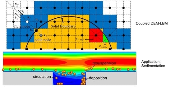
For coupling LBM with DEM, it is of significant importance to properly describe the fluid-solid interactions. The first step is to establish a lattice discretisation of the solid particle on the lattice grid. As illustrated in Figure 3, four types of lattice nodes are obtained as: (1) the pure fluid node without connection to any pure solid node; (2) the pure solid node that is not adjacent to any pure fluid node; (3) the fluid boundary node that is linked with both pure fluid node and solid boundary node; and (4) the solid boundary node that is connected with both fluid boundary node and pure solid node. Obviously, it becomes very easy and straightforward to handle any shaped particles with the discrete lattice representation. Hence, there was a variety of techniques with different levels of complexity and accuracy to compute the fluid-solid interaction, including the modified bounce-back (MBB) scheme [65,66], interpolated bounce-back (IBB) scheme [67,68,69,70,71,72] and immersed boundary methods (IBM) [73,74,75,76,77,78,79,80,81].
4.1. Modified Bounce-Back Scheme
The MBB scheme was proposed by Ladd [65,66] in order to improve the simple bounce-back rules to incorporate the influence of moving fluid-solid interfaces. As shown in Figure 3, this method assumes that the exact solid surface lies halfway between fluid boundary node and solid boundary node, where the bounce-back condition is enforced. The particle is treated as a shell full of fluid. Therefore, the bounce-back takes place on both side of the fluid-solid interface.
The first step is to estimate the velocity at the fluid-solid interface based on the solid particle’s velocity, which is given as:
where Xp is centre of the solid particle. Then the undetermined distribution functions at the fluid boundary node and solid boundary node are computed respectively, according to the modified bounce-back rule,
It can be seen that Equation (27) reduces to the simple bounce-back scheme (Equation (25)) when vb = 0. Once the bounce-back procedure is accomplished, the hydrodynamic force on the solid particle at this particular boundary node is calculated with the momentum exchange method,
The total hydrodynamic force and torque are computed by summing up the contributions from every lattice speed direction and boundary node,
Apparently, the discrete representation of the solid particle surface on the lattice grid is in a stepwise fashion. It is reported that the accuracy of MBB is of first order only due to the zig-zag staircases of a curved surface. Large fluctuations of the hydrodynamic interactions are also observed. Using a sufficiently high lattice resolution could provide much more smooth and accurate force evaluations, which, however, will lead to a huge increase of the computational cost. To overcome these drawbacks of MBB, several improved techniques were proposed, which will be introduced below.
4.2. Interpolated Bounce-Back Scheme
To precisely describe the actual boundary of the solid particle, several bounce-back schemes using the spatial interpolation were also proposed [67,68,69,70,71,72]. In all these techniques, the relative location of the exact fluid-solid interface is interpolated with a location parameter q. Hence more accurate and smoother evaluations of the hydrodynamic force and torque are obtained, which is demonstrated to maintain the second-order accuracy. Here a double interpolation scheme proposed by Yu et al. [71,72] is introduced to show how these schemes work. As shown in Figure 4, the undetermined distribution function is the one coming out of the solid boundary f−i(xf, t + Δt). In most of time, the solid boundary is not exactly located on a lattice node. Then the relative location of the solid boundary can be described by a weighting parameter q by means of spatial interpolation,
where xs, xb and xf represent the positions of the solid node, the solid boundary and the first fluid node next to the solid boundary, respectively. The weighting parameter q varies between 0 and 1. When q = 0, the solid boundary is exactly located on the nearest fluid node, which is turned into a solid node. When q = 1, the solid boundary lies just on the nearest solid node. Then the density function at the temporary location xb that propagates exactly to the solid boundary during the streaming process can be interpolated with the existing density functions fi(xf, t + Δt) and fi(xff, t + Δt), through a first order form,
Next, a bounce-back operation takes place instantaneously at the solid boundary as:
which is the same as the MBB described in Equation (27). In the last step, the unknown density function f−i(xf, t + Δt) is determined from f−i(xb, t + Δt) and f−i(xff, t + Δt) through a first order interpolation,
It should be noted that the interpolation can also be performed with second order form, where the density function from further fluid node xfff is needed. The force and torque on the solid particle can be evaluated similarly with a momentum exchange method,
4.3. Immersed Moving Boundary Method
The immersed boundary method (IBM) was proposed by Peskin [73,74] and further implemented in LBM by other researchers [75,76,77,78,79,80]. In this method, extra moving Lagrangian nodes are introduced to represent the solid particle shape, which are assumed to be deformable with a large stiffness. The effects of the immersed particle boundary on the fluid are modelled by restoring forces based on the ‘no-slip’ boundary condition, which tend to keep the particle to its original shape. Then the restoring forces are distributed to their surrounding fluid nodes and considered as the external force terms in the governing equations. The drawbacks of the IBM include the introduction of additional free parameters, the problem-sensitive determination of the spring stiffness and the damping constant, as well as the severely restricted computational time step.
As an alternative, Noble and Torczynski [81] proposed an immersed moving boundary technique based on the local solid fraction in each lattice cell, which is also known as the partially-solid scheme. This method not only overcomes the momentum discontinuity of MBB-based techniques and provides an adequate representation of complex boundaries at relative lower lattice resolutions, but also retains the prominent advantages of the LBM, i.e., the simple linear collision operator and its locality in computation. In this method, the lattice Boltzmann equation is modified to include an additional collision term, which depends on the local volume fraction of solid (see Figure 3 right part),
where Bn is a total weighting function in each lattice cell, Bs is the weighting function from each solid particle in the same lattice cell, and Ωis is the additional collision term. The total weighting function is calculated by summing up the weighting function of each solid particle that intersect with the same lattice cell such that . Each particle’s weighting function is determined by its own solid fraction and the relaxation parameter as:
where εs is the corresponding particle’s solid fraction and εn is total solid fraction in the same lattice cell that is the sum of each particle’s contribution, i.e., . It can be seen that when the solid fraction εs varies from 0 (a completely fluid cell) to 1 (a completely solid cell), Bs varies from 0 to 1. Equation (35) returns to the original SRT-LBE for pure fluid when Bs = 0, and returns the new collision operator plus the distribution from the previous time step when Bs = 1. The new collision operator is given by
The total hydrodynamic force and torque acting on the solid particle can be evaluated using the momentum exchange method with the additional collision operator over all lattice directions at each node and then over all fluid boundary, solid boundary and internal solid nodes, which are expressed as:
Note that the implementation of the immersed moving boundary method is straightforward. Only quantities already available in the lattice cell or easily derived are used. No additional data storage or organization is needed, which is a crucial advantage over other moving boundary techniques. However, it is also noticed that the critical step in this method is the calculation of the solid fraction in each lattice cell, which is primarily a geometry problem. Many methods are proposed to estimate the solid coverage ratio of a geometry with a square or a cube, including analytically solution, Monte Carlo sampling technique, cell decomposition method, polygonal approximation, edge-intersection averaging method, linear approximation and so on [82,83]. In the current LBM-DEM numerical framework, the analytical solution is used for 2D problems, while for 3D a linear approximation method is adopted, in order to save computational cost but still retain relatively accurate results.
4.4. Time Steps in the LBM-DEM Coupling
The time step coupling is also a crucial issue in the LBM-DEM coupling [31,82]. As we discussed previously, the time step of LBM is generally set as a dimensionless value of one in the computation. The real physical time is implicitly determined by computational parameters as well as the unit conversion scheme. Based on Li and Marshall’s work [3,58], the DEM time step depends on the interparticle collision time scale,
which typically varies around 10−6 ~ 10−9 s. Therefore, it is believed that the LBM time step is generally larger than the DEM time step. A time step ratio λ is then introduced as ΔtLBM = λΔtDEM, which can be decided after all the parameters are settled. It should be noted that the time step ratio λ could be either greater or lower than one. If λ < 1, the critical time step can be simply set as ΔtLBM, and the DEM time step can be equal to ΔtLBM. When λ > 1, a number of DEM computation steps are performed within one LBM time step, during which the fluid forces and torques are kept unchanged.
5. Validation
In this section, a few validation studies are performed to demonstrate the accuracy of our LBM-DEM numerical approach, including single-phase Poiseuille flow, gravitational settling of a particle, and the drag force on a stationary particle.
5.1. Poiseuille Flow
Single-phase Poiseuille flows in both 2D and 3D are first analysed using the LBM-DEM. The validation is performed with both SRT and MRT models. As shown in Figure 5, the boundaries in are periodic, and y-direction are bounded by two ‘no-slip’ walls. A constant pressure gradient is imposed in the channel in x-direction to drive the flow. The channel size is H × H for the 2D case and 10 × H × H for the 3D case. A few lattice resolutions are selected in the range H = 11 ~ 101 to examine the convergence of the numerical model. The relaxation parameter is fixed at 0.65. Different channel Reynolds numbers are achieved by changing the magnitude of the body force. Figure 6 and Figure 7 show the normalised velocity profiles for 2D and 3D Poiseuille flow, respectively. The L-2 norm calculation is used to compute the relative error:
where U is the flow velocity obtained from the simulation and Utheory is the analytical solution of the Poiseuille flow [84]. It can be inferred that the numerical results agree very well with the theoretical prediction. The accuracy is second order for the 2D flow, while it is slightly lower than second order for the 3D duct flow.
5.2. Gravitational Settling of a Particle
For gravitational settling of a particle, both 2D and 3D cases are simulated to evaluate the validity of our numerical approach in a dynamic system. This validation is performed with SRT-LBM along with the Hertz model in DEM. For the 2D case, the computational setup is identical to that in Wen et al.’s work [85]. As shown in Figure 8, a cylinder with diameter dp = 0.1 cm is initially located 0.076 cm away from the left wall of a vertical channel with width 0.4 cm. The fluid density and kinematic viscosity are 1000 kg/m3 and 1 × 10⁻⁶m2/s, respectively. The mass density of the cylinder is 1030 kg/m3. Therefore, the cylinder will settle under the gravitational force and finally reaches a steady state that moves along the centreline at a constant velocity. The computational setup in the lattice unit scheme is as follows. The size of the channel is nx × ny = 121 × 1201 and ‘no-slip’ wall boundaries are imposed on all the four faces. The cylinder’s diameter and mass density are dp = 30 and ρp = 1.03, respectively. The dimensionless relaxation parameter is set as 0.6. Note that the IBM is applied in the solid–fluid coupling in this particular problem.
A detailed comparison between the present numerical results and that obtained by the arbitrary Lagrangian–Eulerian technique (ALE) [85] is presented in Figure 9, where very good agreement is reached. Furthermore, the force profiles are quite smooth without any large fluctuations.
For the 3D case, the single particle settling experiment reported by Ten Cate et al. [86] is numerically reproduced. A spherical particle with diameter dp = 15 mm and density ρp = 1,120 kg/m3 is initially released from a height h = 120 mm in a cuboid box with a size of 100 × 100 × 160 mm3. The box is full of silicon oil, and four different types of oil are used in the experiment. The densities and dynamic viscosities of the silicon oil are ρf = 970, 965, 962, 960 kg/m3 and νf = 373, 212, 113, 58 Pa·s, respectively. The terminal settling velocity of the particle in the four oils are uter = 0.038, 0.060, 0.091, 0.128 m/s, respectively, which results in four different particle Reynolds number Rep = 1.5, 4.1, 11.6, 31.9, respectively. The computational parameters in the dimensionless lattice unit are given below. The domain size is 51 × 51 × 81 and the particle diameter is dp = 7.5. The density of the fluid is fixed at ρf = 1.0, so that the corresponding particle density is ρp = 1.155, 1.161, 1.164, and 1.167 for different fluids considered, respectively. The relaxation parameter is set as 0.65. Figure 10 shows the time evolution of particle trajectory and velocity profiles for different Reynolds numbers. It is apparent that the numerical results are in excellent agreement with the experimental results, which further demonstrates the validity and accuracy of the present numerical approach.
5.3. Drag Force on a Stationary Particle
The classical drag force problem is also simulated to verify the accuracy of the force evaluation in our LBM-DEM coupling, which is carried out with the SRT-LBM. As depicted in Figure 11, a circular (spherical) particle is placed in the centre of a rectangular (cuboid) domain and kept stationary. The domain size is L × H = 50dp × 50dp in 2D and L × H × H = 20dp × 10dp × 10dp in 3D. The inlet boundary is constant flow with velocity U0 and the outlet is set as constant pressure boundary. All the other boundaries are set as open boundary (zero gradient). The particle Reynolds number and the drag coefficient are calculated as
where Fd is the fluid drag force on the particle. Note that both the IBB and IBM are used in the drag force validation.
Figure 12 shows the drag coefficient Cd as a function of the particle Reynolds number Rep for both 2D and 3D cases. For the 2D case shown in Figure 12a, the experimental results reported by Tritton are also superimposed for comparison [87]. It is clear that both the results obtained by IBB and IBM agree well with the experiments. Second order accuracy of the force evaluation is achieved for IBM, while the accuracy for IBB is lower than second order but higher than first order. For the 3D case shown in Figure 12a,b widely accepted empirical law of the drag coefficient is introduced to serve as the theoretical prediction [88]
We can see that the simulation results agree well with the above theoretical prediction, which demonstrates the validity and accuracy of our coupled LBM-DEM. Furthermore, it is noticed that accurate drag coefficients are obtained using both IBB and IBM even with a relatively low size resolution dp = 6, implying that acceptable accuracy can still be retained when the computational cost is reduced.
6. LBM-DEM Applications
In this section, a few numerical examples are presented to demonstrate the capability of LBM-DEM, which include inertial migration of dense particle suspensions, agglomeration of adhesive particles in channel flow, and sedimentation of particle suspensions in a cavity flow.
6.1. Inertial Migration of Dense Particle Suspensions
In an experimental study of pipe flow of a dilute suspension consisting of neutrally buoyant particles, Segré and Silberberg [89,90] first observed that the particle suspensions tend to migrate laterally and focus in an annulus at radial position r ≈ 0.6R, with R being the pipe radius. This phenomenon is named as the tubular pinch effect (or the Segré–Silberberg effect). Due to the lack of theoretical explanation at the time when it was discovered, this interesting phenomenon prompted a great deal of interest to further explore the underlying mechanism. Since then, many studies were carried out on this fascinating phenomenon experimentally [91,92,93,94,95], theoretically [96,97,98,99] and computationally [100,101,102,103,104,105,106]. The lateral focusing of the particle suspensions is found to be closely related to the fluid inertia. It is well recognised that the lateral migration exists in both 2D and 3D flows, and the equilibrium position moves closer to the wall as the channel Reynolds number increases, which is successfully described with the theoretical solution based on the perturbation theory and the asymptotic expansion method. However, most of the previous works are limited to very dilute suspensions with a particle concentration lower than 1%. When the particle concentration is increased, whether the lateral focusing phenomenon still exists remains less explored. Therefore, the coupled LBM-DEM is employed in the current study to explore this problem.
As shown in Figure 13, let us consider a pressure-driven flow of non-Brownian particle suspensions in a 2D channel. Periodic boundary conditions are applied in x-direction and the top and bottom planes in y-direction are set as ‘no-slip’ walls. The particles are neutrally buoyant, i.e., the fluid and the particle have the same mass density. The particles’ initial positions are randomly generated inside the channel at the beginning of the simulation. Driven by the pressure gradient, the particle suspensions will transport and migrate to their equilibrium positions. A steady particle–fluid flow is expected after a sufficient long time of computation. The parameters used in the simulation are as follows. The size of the channel is L × H = 501 × 101. The particle diameter is dp = 6 and 12. The particle concentration ϕ ranges between 1% and 50%. The channel Reynolds number Re0 is tuned in the range 4 ~ 100 by varying the pressure gradient. Note that the channel Reynolds number refers to the one under a single phase flow with no particles. The SRT model and the Hertz contact model are used in the LBM and DEM for this particular problem, respectively.
Figure 14 displays the snapshots of the particle suspension with different channel Reynolds numbers, where the particle concentration is fixed at ϕ = 10%. It is observed that only a small part of the particles undergoes the lateral migration at a relatively small Reynolds number Re0 = 4. As Re0 increases, a complete migration takes place at both Re0 = 40 and Re0 = 100, where all the particles are focused at a certain lateral position. Furthermore, it is found out that the larger Re0 is, the shorter time it takes to develop into a full migration. For example, it occurs around t = 5.5 × 10⁴ for Re0 = 40, while it is much earlier around t = 4 × 10⁴ for Re0 = 100. Figure 15 illustrates the effects of particle concentration on the particle migration. It is clear that with relatively low particle concentration (ϕ = 1% and 10%), the lateral migration is still notable. However, as ϕ increases to 40%, the migration is dramatically suppressed and the particle suspensions appear to jam near the wall.
To quantify the influence of the particle concentration, the degree of inertial migration can be defined as [94],
which estimates the total probability distribution function (PDF) of the particles in the upper and lower quarter of the channel. Since the lateral equilibrium position is around 0.6 according to the Segré and Silberberg effect, the degree of the migration must be Pf = 1 if all the particles are laterally focused. On the other hand, if the particle suspension remains randomly distributed in the channel, Pf is expected to be 0.5. Figure 16 shows the variation of the degree of inertial migration with particle concentration for different dp and Re0. It is observed that Pf equals one for all the Re0 at a low particle concentration (ϕ ≤ 5%), while Pf remains around 0.5 ~ 0.6 at ϕ = 50% for all the Re0, implying a huge impact of the particle concentration on the lateral migration. A full migration is always accessible when the particle suspension is not dense, but it is completely suppressed with a very large particle concentration for the range of Re0 in the present study. However, when ϕ is between 5% and 50%, the variation of Pf strongly depends on Re0. With a fixed ϕ, a larger Re0 leads to a larger Pf, i.e., a higher degree of lateral migration.
The above discussion reveals that the degree of the migration is determined by the particle concentration and channel Reynolds number. A dimensionless focusing number was proposed to characterise the degree of migration [37],
where m = 0.36 and n = 2.33 are obtained from the fitting of simulation data. Figure 17 shows the degree of migration Pf as a function of the focusing number Fc, where an empirical fitting is given by an exponential equation . It can be seen that the numerical results coalesce onto a single master curve and three distinct regimes can be identified based on the value of Fc: a laterally unfocused regime (Fc < 30), a partially migration regime (30 < Fc < 300) and a fully migration regime (Fc > 300).
6.2. Agglomeration of Adhesive Particles in Channel Flow
The inertial focusing introduced in the previous section has prompted a variety of novel applications in the microfabrication, such as particle filtration, segregation and flow cytometry in the micro channels [107,108,109]. An inevitable problem of particle agglomeration due to the cohesive nature when the size reduces to the micron scale must be taken into consideration. The agglomeration is ubiquitous in nature and industry, and sometimes will cause unfavourable effects in industrial facility. For example, the agglomeration of asphaltenes or gas hydrates results in the pipeline blockage in the oil and gas engineering [110,111]. Therefore, it is worth investigating the fundamental mechanism of micro-particle agglomeration.
As displayed in Figure 18, a stream of dilute particle suspension flowing through a 3D square channel is considered. Periodic boundary conditions are imposed at the inlet and outlet, while other four faces of the channel are set as ‘no-slip’ walls. The flow is driven by a constant pressure gradient. The particles are neutrally buoyant and adhesive, with initial positions randomly distributed in the channel. The computational parameters are set as follow. The dimension of the channel is L × H × H = 201 × 61 × 61. By varying the pressure gradient, the channel Reynolds number ranges between 5.4 and 108. The particle size is dp = 5 and the particle concentration is fixed at 1%, corresponding to a particle number of 110. The strength of the particle adhesion is represented by the surface energy, which is chosen as 0.075 and 0.0075. The SRT model and the JKR contact theory are used in the LBM and DEM for this problem, respectively.
Figure 19 and Figure 20 display the snapshots of adhesive particle suspensions with different surface energies γ = 0.075 and γ = 0.0075, respectively. It can be found that large sized agglomerates are formed with relatively higher surface energy (γ = 0.075). Some particles even stick on the wall due to strong adhesion. However, when the surface energy is reduced by one order of magnitude (γ = 0.0075), the size of the agglomerates becomes smaller and the particles appear to focus around a certain lateral position with Re = 54 and 108 (see Figure 20c,d), which resembles the Segré-Silberberg effect as discussed in the last section.
Figure 21 shows the lateral PDF of the particle suspensions based on the following definition,
where N is the total number of particles in the channel and N(l, l+Δl) is the number of particles in the square annulus between l and l + Δl. For comparison, the channel flow with non-adhesive particles is also modelled and the results are included. It can be seen from Figure 21a that a single peak at the lateral position around 0.6 is observed in the PDF for non-adhesive particles, which moves closer to the wall as Re increases and is in consistent with the Segré and Silberberg effect. However, the PDFs are quite distinct for adhesive particles. The single peak distribution is not clearly observed for particles with γ = 0.075 (see Figure 21b). Moreover, there appears to be a peak close to the wall position, where a number of particles are found to stick to wall because of the strong adhesion, as indicated by Figure 19. On the other hand, for much less adhesive particles (γ = 0.0075), the PDFs become similar to those of non-adhesive particles (see Figure 21c). The average lateral position as a function of Re is further shown in Figure 22. Note that the relatively larger value of average lateral position for Re = 5.4 is caused by the statistical effect [38], because the fluid inertia is relatively small to drive the lateral migration and the particles almost remain randomly distributed in the cross-sectional area. Except for the data for Re = 5.4, it is observed that the average lateral position increases monotonically with the increase of Re for both non-adhesive and less adhesive particles (γ = 0.0075), which demonstrates a similar dynamics between non-adhesive and weak adhesive particles. However, for strongly adhesive particles (γ = 0.075), the monotonic increase of the average lateral position disappears because of the agglomeration.
The agglomeration mechanism for such channel flow can be attributed to the competition between the interparticle adhesive contact force and the hydrodynamic force. The adhesive force sticks particles together, which imposes a positive effect on the agglomeration. The hydrodynamic force exerts two opposite effects on the particle suspensions. First, it induces the particle lateral migration, which motivates the interparticle collision and facilitates the agglomeration. Secondly, the fluid inertia also tears particles apart from each other, resulting in the breakup of agglomerates. As a consequence, a new dimensionless adhesion number Ad is proposed based on the balance of the critical pull-off force and the drag force [11,12,38],
where μf is the fluid dynamic viscosity and U is the mean fluid velocity. Using the adhesion number, the degree of the agglomeration can be characterised and represented by the agglomerate ratio that is defined as the ratio of the number of particles involved in agglomerate to the total particle number. Figure 23 shows the relationship between the agglomerate ratio and the adhesion number. A monotonic increase of the agglomerate ratio as a function of Ad is observed. After Ad reaches a critical value, the agglomerate ratio seems to converge to one. Therefore, two different regimes can be identified, i.e., a partial agglomeration regime where the hydrodynamic force dominates over the adhesive force, and a complete agglomeration regime where all the particles are involved in agglomerates.
6.3. Sedimentation of Particle Suspensions in Cavity Flow
Sedimentation is extensively used in industries to separate particles from fluid or other particles with different sizes or velocities, such as separating particles and cells in microfluids [112], dewatering coal slurries [113], and post-treating wastewater [114,115,116]. Furthermore, sediments are also physical pollutants in the river, which could have great influence on the ecosystem and human health [117,118,119,120]. Therefore, it is of great importance to study the sedimentation, which is a very complicated process, due to the complex fluid mechanics involved with the sediment particles. With LBM-DEM, a numerical investigation is then performed to gain some insights to the sedimentation problem.
As shown in Figure 24, we consider a sedimentation system composed of a cuboid channel and a cavity, which is placed in the middle of the channel. The boundaries in x and y directions are periodic, and all the other faces are set as no-slip walls. The particles are initially generated at random positions in the main channel (no particles in the cavity). The particle density is larger than the fluid, so that they can sedimentate into the cavity under the gravity. The size of the main channel is L × W × H = 321 × 81 × 49. The cavity has the same width as the main channel. The length of the cavity is l = 40 and 80, while the height is h = 16 and 32, which gives rise to four configurations of the cavity. The channel Reynolds number, defined as Re = UxH/ν varies between 28.44 and 88.32. The particle diameter is dp = 6 and the density is in the range 1.1 ~ 2.0. The total number of particles is fixed at 110, which is equal to an overall concentration less than 1%. The SRT model and the Hertz model are used in the LBM and DEM for this particular problem, respectively.
Figure 25 shows the snapshots of the particle suspensions at different time. The particles are initially located at random positions in the main channel with no particles trapped inside the cavity. Then the particles settle to the bottom of the channel and flow over the cavity. During the transportation of the suspensions, some particles fall into the cavity and stay stationary inside, while some other keep circulating around an orbit in the central vortex inside the cavity. The total number of particles trapped inside the cavity is evaluated after a sufficiently long time, when the transportation of the particles reaches a steady state. From Figure 25 the typical trajectories of particle suspensions in the cavity are analysed, where three distinct dynamic behaviours can be identified: resuspension, deposition and circulation. Resuspension means that the particles fall into the cavity and then come out due to the lift force from the fluid. Deposition happens mostly at the rear edge of the cavity, where the particles deposit to the corner of the cavity and stay motionless. Circulation indicates that the particles are captured by the central vortex inside the cavity and keeps moving along an orbit in a periodic way. Both deposition and circulation are treated as the entrapment of a particle.
Figure 26 shows the trap efficiency η, defined as the ratio of the trapped particle number to the total particle number, as a function of the particle density for different cavity configurations and Reynolds numbers. It is clear that as the particle density increases, the trap efficiency increases continuously from 0 to 1. For a fixed Reynolds number, the largest cavity (h = 32, l = 80) has the highest trap efficiency, while the smallest cavity (h = 16, l = 40) has the lowest trap efficiency. The results of the other two cavity configurations are in between, which indicates that increasing either length or depth leads to a higher trap efficiency. Furthermore, for a fixed cavity configuration, an increase in the Reynolds number results in a decrease in the trap efficiency. With a larger Reynolds number, the particle’s translational velocity in x direction becomes larger, so that it has less time to enter the cavity in the vertical direction. Meanwhile, a larger Reynolds number produces a larger lift force. As a consequence, the particles are less easily trapped in the cavity.
7. Summary
An overview of the coupled discrete element method with the lattice Boltzmann method is presented together with its applications in solid–liquid flows. The fundamentals of DEM and LBM, including the contact mechanics based on Hertz model and JKR theory, the lattice Boltzmann equation with both single-relaxation-time model and multi-relaxation-time model are introduced. Several solid–fluid interaction models, i.e., the coupling between DEM and LBM, are discussed and compared in detail. The validity and accuracy of the numerical method are validated for three classical solid–liquid flow problems, and the results are in good quantitative agreement with those from experiments and other numerical approaches. Three case studies, including the inertial migration of particle suspensions, the agglomeration of adhesive particles, and the sedimentation problem, are also performed to demonstrate the capability of the coupled DEM-LBM to solid–liquid flow problems and potential engineering applications.
Author Contributions
Conceptualization, C.-Y.W.; formal analysis, W.L.; funding acquisition, C.-Y.W.; methodology, W.L. and C.-Y.W.; project administration, C.-Y.W.; supervision, C.-Y.W.; validation, W.L.; writing—original draft, W.L.; writing—review and editing, C.-Y.W. All authors have read and agreed to the published version of the manuscript.
Funding
This research was funded by the Engineering and Physical Sciences Research Council (EPSRC), grant number No: EP/N033876/1.
Acknowledgments
The authors acknowledge Duo Zhang and Nicolin Govender in the University of Surrey for their helpful suggestions and fruitful discussion in developing the numerical approach.
Conflicts of Interest
The authors declare no conflict of interest.
References
- Zhu, H.; Zhou, Z.; Yang, R.; Yu, A. Discrete particle simulation of particulate systems: Theoretical developments. Chem. Eng. Sci. 2007, 62, 3378–3396. [Google Scholar] [CrossRef]
- Zhu, H.; Zhou, Z.; Yang, R.; Yu, A. Discrete particle simulation of particulate systems: A review of major applications and findings. Chem. Eng. Sci. 2008, 63, 5728–5770. [Google Scholar] [CrossRef]
- Li, S.; Marshall, J.S.; Liu, G.; Yao, Q. Adhesive particulate flow: The discrete-element method and its application in energy and environmental engineering. Prog. Energy Combust. Sci. 2011, 37, 633–668. [Google Scholar] [CrossRef]
- Hounslow, M.; Ryall, R.L.; Marshall, V.R. A discretized population balance for nucleation, growth, and aggregation. AIChE J. 1988, 34, 1821–1832. [Google Scholar] [CrossRef]
- Lister, J.D.; Smit, D.J.; Hounslow, M. Adjustable discretized population balance for growth and aggregation. AIChE J. 1995, 41, 591–603. [Google Scholar] [CrossRef]
- Gidaspow, D. Multiphase Flow and Fluidization; Elsevier: Amsterdam, The Netherlands, 1994. [Google Scholar]
- Zhu, R.; Zhu, W.; Xing, L.; Sun, Q. DEM simulation on particle mixing in dry and wet particles spouted bed. Powder Technol. 2011, 210, 73–81. [Google Scholar] [CrossRef]
- Liu, G.; Li, S.; Yao, Q. A JKR-based dynamic model for the impact of micro-particle with a flat surface. Powder Technol. 2011, 207, 215–223. [Google Scholar] [CrossRef]
- Yang, M.; Li, S.; Yao, Q. Mechanistic studies of initial deposition of fine adhesive particles on a fiber using discrete-element methods. Powder Technol. 2013, 248, 44–53. [Google Scholar] [CrossRef]
- Chen, S.; Li, S.; Yang, M. Sticking/rebound criterion for collisions of small adhesive particles: Effects of impact parameter and particle size. Powder Technol. 2015, 274, 431–440. [Google Scholar] [CrossRef]
- Liu, W.; Li, S.; Baule, A.; Makse, H.A. Adhesive loose packings of small dry particles. Soft Matter 2015, 11, 6492–6498. [Google Scholar] [CrossRef] [Green Version]
- Liu, W.; Li, S.; Chen, S. Computer simulation of random loose packings of micro-particles in presence of adhesion and friction. Powder Technol. 2016, 302, 414–422. [Google Scholar] [CrossRef] [Green Version]
- Liu, W.; Jin, Y.; Li, S.; Chen, S.; Makse, H.A. Equation of state for random sphere packing with arbitrary adhesion and friction. Soft Matter 2017, 13, 421–427. [Google Scholar] [CrossRef] [PubMed] [Green Version]
- Liu, W.; Chen, S.; Li, S. Random adhesive loose packings of micron-sized particles under a uniform flow field. Powder Technol. 2018, 335, 70–76. [Google Scholar] [CrossRef]
- Chen, S.; Liu, W.; Li, S. A fast adhesive discrete element method for random packings of fine particles. Chem. Eng. Sci. 2019, 193, 336–345. [Google Scholar] [CrossRef] [Green Version]
- Zhang, H.; Sharma, G.; Wang, Y.; Li, S.; Biswas, P. Numerical modeling of the performance of high flow DMAs to classify sub-2 nm particles. Aerosol Sci. Technol. 2018, 53, 106–118. [Google Scholar] [CrossRef]
- Dong, M.; Li, J.; Shang, Y.; Li, S. Numerical investigation on deposition process of submicron particles in collision with a single cylindrical fiber. J. Aerosol Sci. 2019, 129, 1–15. [Google Scholar] [CrossRef]
- Cundall, P.A.; Strack, O.D.L. A discrete numerical model for granular assemblies. Géotechnique 1979, 29, 47–65. [Google Scholar] [CrossRef]
- Chen, S.; Doolen, G.D. Lattice boltzmann method for fluid flows. Annu. Rev. Fluid Mech. 1998, 30, 329–364. [Google Scholar] [CrossRef] [Green Version]
- Aidun, C.K.; Clausen, J.R. Lattice-Boltzmann Method for Complex Flows. Annu. Rev. Fluid Mech. 2010, 42, 439–472. [Google Scholar] [CrossRef]
- Krüger, T.; Kusumaatmaja, H.; Kuzmin, A.; Shardt, O.; Silva, G.; Viggen, E.M. The Lattice Boltzmann Method; Springer Science and Business Media: Berlin, Germany, 2017; Volume 10, pp. 4–15. [Google Scholar]
- Moin, P.; Mahesh, K. Direct Numerical Simulation: A Tool in Turbulence Research. Annu. Rev. Fluid Mech. 1998, 30, 539–578. [Google Scholar] [CrossRef] [Green Version]
- Sagaut, P. Large Eddy Simulation for Incompressible Flows; Springer Science and Business Media: Berlin, Germany, 2006. [Google Scholar]
- Ishii, M.; Mishima, K. Two-fluid model and hydrodynamic constitutive relations. Nucl. Eng. Des. 1984, 82, 107–126. [Google Scholar] [CrossRef]
- Tsuji, Y.; Kawaguchi, T.; Tanaka, T. Discrete particle simulation of two-dimensional fluidized bed. Powder Technol. 1993, 77, 79–87. [Google Scholar] [CrossRef]
- Kuipers, J.; Van Duin, K.; Van Beckum, F.; Van Swaaij, W. A numerical model of gas-fluidized beds. Chem. Eng. Sci. 1992, 47, 1913–1924. [Google Scholar] [CrossRef] [Green Version]
- Kafui, K.; Thornton, C.; Adams, M. Discrete particle-continuum fluid modelling of gas-solid fluidised beds. Chem. Eng. Sci. 2002, 57, 2395–2410. [Google Scholar] [CrossRef]
- Guo, Y.; Kafui, K.D.; Wu, C.-Y.; Thornton, C.; Seville, J.P.K. A coupled DEM/CFD analysis of the effect of air on powder flow during die filling. AIChE J. 2009, 55, 49–62. [Google Scholar] [CrossRef]
- Guo, Y.; Wu, C.-Y.; Kafui, K.; Thornton, C. 3D DEM/CFD analysis of size-induced segregation during die filling. Powder Technol. 2011, 206, 177–188. [Google Scholar] [CrossRef]
- Guo, Y.; Wu, C.-Y.; Thornton, C. Modeling gas-particle two-phase flows with complex and moving boundaries using DEM-CFD with an immersed boundary method. AIChE J. 2012, 59, 1075–1087. [Google Scholar] [CrossRef]
- Feng, Y.T.; Han, K.; Owen, D.R.J. Coupled lattice Boltzmann method and discrete element modelling of particle transport in turbulent fluid flows: Computational issues. Int. J. Numer. Methods Eng. 2007, 72, 1111–1134. [Google Scholar] [CrossRef]
- Strack, O.E.; Cook, B.K. Three-dimensional immersed boundary conditions for moving solids in the lattice-Boltzmann method. Int. J. Numer. Methods Fluids 2007, 55, 103–125. [Google Scholar] [CrossRef]
- van der Hoef, M.A.; Annaland, M.V.S.; Deen, N.; Kuipers, H. Numerical Simulation of Dense Gas-Solid Fluidized Beds: A Multiscale Modeling Strategy. Annu. Rev. Fluid Mech. 2008, 40, 47–70. [Google Scholar] [CrossRef]
- Van Wachem, B.; Schouten, J.C.; Bleek, C.M.V.D.; Krishna, R.; Sinclair, J.L. Comparative analysis of CFD models of dense gas–solid systems. AIChE J. 2001, 47, 1035–1051. [Google Scholar] [CrossRef]
- Ladd, A.J.C.; Verberg, R. Lattice-Boltzmann Simulations of Particle-Fluid Suspensions. J. Stat. Phys. 2001, 104, 1191–1251. [Google Scholar] [CrossRef]
- Nguyen, N.-Q.; Ladd, A.J.C. Lubrication corrections for lattice-Boltzmann simulations of particle suspensions. Phys. Rev. E 2002, 66, 046708. [Google Scholar] [CrossRef] [PubMed] [Green Version]
- Liu, W. Analysis of inertial migration of neutrally buoyant particle suspensions in a planar Poiseuille flow with a coupled lattice Boltzmann method-discrete element method. Phys. Fluids 2019, 31, 063301. [Google Scholar] [CrossRef]
- Liu, W.; Wu, C.-Y. Migration and agglomeration of adhesive microparticle suspensions in a pressure-driven duct flow. AIChE J. 2020, 66, 16974. [Google Scholar] [CrossRef]
- Maier, R.S.; Kroll, D.M.; Kutsovsky, Y.E.; Davis, H.T.; Bernard, R.S. Simulation of flow through bead packs using the lattice Boltzmann method. Phys. Fluids 1998, 10, 60–74. [Google Scholar] [CrossRef]
- Guo, Z.; Zhao, T. Lattice Boltzmann model for incompressible flows through porous media. Phys. Rev. E 2002, 66, 036304. [Google Scholar] [CrossRef] [PubMed]
- Inamuro, T.; Ogata, T.; Tajima, S.; Konishi, N. A lattice Boltzmann method for incompressible two-phase flows with large density differences. J. Comput. Phys. 2004, 198, 628–644. [Google Scholar] [CrossRef]
- Li, Q.; Luo, K.H.; Kang, Q.; He, Y.; Chen, Q.; Liu, Q. Lattice Boltzmann methods for multiphase flow and phase-change heat transfer. Prog. Energy Combust. Sci. 2016, 52, 62–105. [Google Scholar] [CrossRef] [Green Version]
- Han, Y.; Cundall, P.A. LBM-DEM modeling of fluid-solid interaction in porous media. Int. J. Numer. Anal. Methods Geomech. 2012, 37, 1391–1407. [Google Scholar] [CrossRef]
- Peng, C.; Ayala, O.M.; Wang, L.-P. A direct numerical investigation of two-way interactions in a particle-laden turbulent channel flow. J. Fluid Mech. 2019, 875, 1096–1144. [Google Scholar] [CrossRef] [Green Version]
- Chen, S.; Chen, H.; Martnez, D.; Matthaeus, W. Lattice Boltzmann model for simulation of magnetohydrodynamics. Phys. Rev. Lett. 1991, 67, 3776–3779. [Google Scholar] [CrossRef] [PubMed]
- Pei, C.; Wu, C.-Y.; England, D.; Byard, S.; Berchtold, H.; Adams, M. DEM-CFD modeling of particle systems with long-range electrostatic interactions. AIChE J. 2015, 61, 1792–1803. [Google Scholar] [CrossRef]
- Pei, C.; Wu, C.-Y.; Adams, M.; England, D.; Byard, S.; Berchtold, H. Contact electrification and charge distribution on elongated particles in a vibrating container. Chem. Eng. Sci. 2015, 125, 238–247. [Google Scholar] [CrossRef] [Green Version]
- Pei, C.; Wu, C.-Y.; Adams, M. Numerical analysis of contact electrification of non-spherical particles in a rotating drum. Powder Technol. 2015, 285, 110–122. [Google Scholar] [CrossRef] [Green Version]
- Chen, S.; Li, S.; Liu, W.; Makse, H.A. Effect of long-range repulsive Coulomb interactions on packing structure of adhesive particles. Soft Matter 2016, 12, 1836–1846. [Google Scholar] [CrossRef] [Green Version]
- Chen, S.; Liu, W.; Li, S. Effect of long-range electrostatic repulsion on pore clogging during microfiltration. Phys. Rev. E 2016, 94, 063108. [Google Scholar] [CrossRef]
- Chen, S.; Liu, W.; Li, S. Scaling laws for migrating cloud of low-Reynolds-number particles with Coulomb repulsion. J. Fluid Mech. 2017, 835, 880–897. [Google Scholar] [CrossRef]
- Zhu, R.; Li, S.; Yao, Q. Effects of cohesion on the flow patterns of granular materials in spouted beds. Phys. Rev. E 2013, 87, 022206. [Google Scholar] [CrossRef]
- Zhang, H.; Li, S. DEM simulation of wet granular-fluid flows in spouted beds: Numerical studies and experimental verifications. Powder Technol. 2017, 318, 337–349. [Google Scholar] [CrossRef]
- Chen, H.; Liu, W.; Li, S. Deposition of wet microparticles on a fiber: Effects of impact velocity and initial spin. Powder Technol. 2019, 357, 83–96. [Google Scholar] [CrossRef]
- Hertz, H. Ueber die Berührung fester elastischer Körper. J. für die reine und angewandte Mathematik (Crelles J.) 1882, 1882, 156–171. [Google Scholar] [CrossRef]
- Johnson, K.L.; Kendall, K.; Roberts, A.D. Surface energy and the contact of elastic solids. Proc. R. Soc. London. Ser. A Math. Phys. Sci. 1971, 324, 301–313. [Google Scholar] [CrossRef] [Green Version]
- Derjaguin, B.; Muller, V.; Toporov, Y. Effect of contact deformations on the adhesion of particles. J. Colloid Interface Sci. 1975, 53, 314–326. [Google Scholar] [CrossRef]
- Marshall, J.S.; Li, S. Adhesive Particle Flows; Cambridge University Press (CUP): Cambridge, UK, 2014. [Google Scholar]
- Bhatnagar, P.L.; Gross, E.P.; Krook, M. A Model for Collision Processes in Gases. I. Small Amplitude Processes in Charged and Neutral One-Component Systems. Phys. Rev. 1954, 94, 511–525. [Google Scholar] [CrossRef]
- Chen, H.; Chen, S.; Matthaeus, W.H. Recovery of the Navier-Stokes equations using a lattice-gas Boltzmann method. Phys. Rev. A 1992, 45, R5339–R5342. [Google Scholar] [CrossRef] [PubMed]
- Qian, Y.H.; D’Humières, D.; Lallemand, P. Lattice BGK Models for Navier-Stokes Equation. EPL (Europhysics Lett.) 1992, 17, 479–484. [Google Scholar] [CrossRef]
- Wolf-Gladrow, D.A. Lattice-Gas Cellular Automata and Lattice Boltzmann Models: An Introduction; Springer: New York, NY, USA, 2004. [Google Scholar]
- Guo, Z.; Zheng, C.; Shi, B. Discrete lattice effects on the forcing term in the lattice Boltzmann method. Phys. Rev. E 2002, 65, 046308. [Google Scholar] [CrossRef]
- Lallemand, P.; Luo, L.-S. Theory of the lattice Boltzmann method: Dispersion, dissipation, isotropy, Galilean invariance, and stability. Phys. Rev. E 2000, 61, 6546–6562. [Google Scholar] [CrossRef] [Green Version]
- Ladd, A.J.C. Numerical simulations of particulate suspensions via a discretized Boltzmann equation. Part 1. Theoretical foundation. J. Fluid Mech. 1994, 271, 285. [Google Scholar] [CrossRef] [Green Version]
- Ladd, A.J.C. Numerical simulations of particulate suspensions via a discretized Boltzmann equation. Part 2. Numerical results. J. Fluid Mech. 1994, 271, 311. [Google Scholar] [CrossRef] [Green Version]
- Bouzidi, M.; Firdaouss, M.; Lallemand, P. Momentum transfer of a Boltzmann-lattice fluid with boundaries. Phys. Fluids 2001, 13, 3452–3459. [Google Scholar] [CrossRef]
- Filippova, O.; Hänel, D. Grid Refinement for Lattice-BGK Models. J. Comput. Phys. 1998, 147, 219–228. [Google Scholar] [CrossRef]
- Mei, R.; Luo, L.-S.; Shyy, W. An Accurate Curved Boundary Treatment in the Lattice Boltzmann Method. J. Comput. Phys. 1999, 155, 307–330. [Google Scholar] [CrossRef]
- Mei, R.; Shyy, W.; Yu, D.; Luo, L.-S. Lattice Boltzmann Method for 3-D Flows with Curved Boundary. J. Comput. Phys. 2000, 161, 680–699. [Google Scholar] [CrossRef] [Green Version]
- Yu, D.; Mei, R.; Luo, L.-S.; Shyy, W. Viscous flow computations with the method of lattice Boltzmann equation. Prog. Aerosp. Sci. 2003, 39, 329–367. [Google Scholar] [CrossRef]
- Peng, C.; Teng, Y.; Hwang, B.; Guo, Z.; Wang, L.-P. Implementation issues and benchmarking of lattice Boltzmann method for moving rigid particle simulations in a viscous flow. Comput. Math. Appl. 2016, 72, 349–374. [Google Scholar] [CrossRef] [Green Version]
- Peskin, C.S. Numerical analysis of blood flow in the heart. J. Comput. Phys. 1977, 25, 220–252. [Google Scholar] [CrossRef]
- Peskin, C.S. The immersed boundary method. Acta Numer. 2002, 11, 479–517. [Google Scholar] [CrossRef] [Green Version]
- Feng, Z.-G.; Michaelides, E.E. The immersed boundary-lattice Boltzmann method for solving fluid–particles interaction problems. J. Comput. Phys. 2004, 195, 602–628. [Google Scholar] [CrossRef]
- Uhlmann, M. An immersed boundary method with direct forcing for the simulation of particulate flows. J. Comput. Phys. 2005, 209, 448–476. [Google Scholar] [CrossRef] [Green Version]
- Breugem, W.-P. A second-order accurate immersed boundary method for fully resolved simulations of particle-laden flows. J. Comput. Phys. 2012, 231, 4469–4498. [Google Scholar] [CrossRef]
- Favier, J.; Revell, A.; Pinelli, A. A Lattice Boltzmann–Immersed Boundary method to simulate the fluid interaction with moving and slender flexible objects. J. Comput. Phys. 2014, 261, 145–161. [Google Scholar] [CrossRef] [Green Version]
- Valero-Lara, P.; Igual, F.D.; Prieto, M.; Pinelli, A.; Favier, J. Accelerating fluid–solid simulations (Lattice-Boltzmann & Immersed-Boundary) on heterogeneous architectures. J. Comput. Sci. 2015, 10, 249–261. [Google Scholar] [CrossRef] [Green Version]
- Valero-Lara, P.; Pinelli, A.; Prieto, M. Accelerating Solid-fluid Interaction using Lattice-boltzmann and Immersed Boundary Coupled Simulations on Heterogeneous Platforms. Procedia Comput. Sci. 2014, 29, 50–61. [Google Scholar] [CrossRef] [Green Version]
- Noble, D.R.; Torczynski, J.R. A Lattice-Boltzmann Method for Partially Saturated Computational Cells. Int. J. Mod. Phys. C 1998, 9, 1189–1201. [Google Scholar] [CrossRef]
- Owen, D.R.J.; Leonardi, C.R.; Feng, Y. An efficient framework for fluid-structure interaction using the lattice Boltzmann method and immersed moving boundaries. Int. J. Numer. Methods Eng. 2010, 87, 66–95. [Google Scholar] [CrossRef]
- Jones, B.D.; Williams, J.R. Fast computation of accurate sphere-cube intersection volume. Eng. Comput. 2017, 34, 1204–1216. [Google Scholar] [CrossRef]
- Sutera, S.P.; Skalak, R. The history of Poiseuille’s law. Annu. Rev. Fluid Mechan. 1993, 25, 1–20. [Google Scholar] [CrossRef]
- Wen, B.; Zhang, C.; Tu, Y.; Wang, C.; Fang, H. Galilean invariant fluid–solid interfacial dynamics in lattice Boltzmann simulations. J. Comput. Phys. 2014, 266, 161–170. [Google Scholar] [CrossRef] [Green Version]
- Cate, A.T.; Nieuwstad, C.H.; Derksen, J.J.; Akker, H.V.D. Particle imaging velocimetry experiments and lattice-Boltzmann simulations on a single sphere settling under gravity. Phys. Fluids 2002, 14, 4012–4025. [Google Scholar] [CrossRef]
- Tritton, D.J. Experiments on the flow past a circular cylinder at low Reynolds numbers. J. Fluid Mech. 1959, 6, 547. [Google Scholar] [CrossRef]
- Schiller, L.; Naumann, A. A drag coefficient correlation. Z. des Ver. Deutsch. Ing. 1935, 77, 318–320. [Google Scholar]
- Segre, G.; Silberberg, A. Behaviour of macroscopic rigid spheres in Poiseuille flow Part 1. Determination of local concentration by statistical analysis of particle passages through crossed light beams. J. Fluid Mech. 1962, 14, 115–135. [Google Scholar] [CrossRef]
- Segre, G.; Silberberg, A. Behaviour of macroscopic rigid spheres in Poiseuille flow Part 2. Experimental results and interpretation. J. Fluid Mech. 1962, 14, 136–157. [Google Scholar] [CrossRef]
- Han, M.; Kim, C.; Kim, M.; Lee, S. Particle migration in tube flow of suspensions. J. Rheol. 1999, 43, 1157–1174. [Google Scholar] [CrossRef]
- Matas, J.-P.; Morris, J.F.; Guazzelli, É. Inertial migration of rigid spherical particles in Poiseuille flow. J. Fluid Mech. 2004, 515, 171–195. [Google Scholar] [CrossRef] [Green Version]
- Di Carlo, D.; Irimia, D.; Tompkins, R.G.; Toner, M. Continuous inertial focusing, ordering, and separation of particles in microchannels. Proc. Natl. Acad. Sci. USA 2007, 104, 18892–18897. [Google Scholar] [CrossRef] [Green Version]
- Choi, Y.-S.; Seo, K.W.; Lee, S.J. Lateral and cross-lateral focusing of spherical particles in a square microchannel. Lab. Chip 2011, 11, 460–465. [Google Scholar] [CrossRef] [Green Version]
- Seo, K.W.; Kang, Y.J.; Lee, S.J. Lateral migration and focusing of microspheres in a microchannel flow of viscoelastic fluids. Phys. Fluids 2014, 26, 063301. [Google Scholar] [CrossRef] [Green Version]
- Ho, B.P.; Leal, L.G. Inertial migration of rigid spheres in two-dimensional unidirectional flows. J. Fluid Mech. 1974, 65, 365–400. [Google Scholar] [CrossRef]
- Schonberg, J.A.; Hinch, E.J. Inertial migration of a sphere in Poiseuille flow. J. Fluid Mech. 1989, 203, 517. [Google Scholar] [CrossRef] [Green Version]
- Asmolov, E.S. The inertial lift on a spherical particle in a plane Poiseuille flow at large channel Reynolds number. J. Fluid Mech. 1999, 381, 63–87. [Google Scholar] [CrossRef]
- Matas, J.-P.; Morris, J.F.; Guazzelli, É. Lateral force on a rigid sphere in large-inertia laminar pipe flow. J. Fluid Mech. 2009, 621, 59. [Google Scholar] [CrossRef]
- Feng, J.J.; Hu, H.H.; Joseph, D.D. Direct simulation of initial value problems for the motion of solid bodies in a Newtonian fluid. Part 2. Couette and Poiseuille flows. J. Fluid Mech. 1994, 277, 271. [Google Scholar] [CrossRef] [Green Version]
- Yang, B.H.; Wang, J.; Joseph, D.D.; Hu, H.H.; Pan, T.-W.; Glowinski, R. Migration of a sphere in tube flow. J. Fluid Mech. 2005, 540, 109. [Google Scholar] [CrossRef] [Green Version]
- Shao, X.; Yu, Z.; Sun, B. Inertial migration of spherical particles in circular Poiseuille flow at moderately high Reynolds numbers. Phys. Fluids 2008, 20, 103307. [Google Scholar] [CrossRef] [Green Version]
- Inamuro, T.; Maeba, K.; Ogino, F. Flow between parallel walls containing the lines of neutrally buoyant circular cylinders. Int. J. Multiph. Flow 2000, 26, 1981–2004. [Google Scholar] [CrossRef]
- Chun, B.; Ladd, A.J.C. Inertial migration of neutrally buoyant particles in a square duct: An investigation of multiple equilibrium positions. Phys. Fluids 2006, 18, 31704. [Google Scholar] [CrossRef] [Green Version]
- Sun, D.-K.; Bo, Z. Numerical simulation of hydrodynamic focusing of particles in straight channel flows with the immersed boundary-lattice Boltzmann method. Int. J. Heat Mass Transf. 2015, 80, 139–149. [Google Scholar] [CrossRef]
- Hu, J.; Guo, Z. A numerical study on the migration of a neutrally buoyant particle in a Poiseuille flow with thermal convection. Int. J. Heat Mass Transf. 2017, 108, 2158–2168. [Google Scholar] [CrossRef]
- Ookawara, S.; Agrawal, M.; Street, D.; Ogawa, K. Quasi-direct numerical simulation of lift force-induced particle separation in a curved microchannel by use of a macroscopic particle model. Chem. Eng. Sci. 2007, 62, 2454–2465. [Google Scholar] [CrossRef]
- Di Carlo, D. Inertial microfluidics. Lab Chip 2009, 9, 3038. [Google Scholar] [CrossRef] [PubMed]
- Ahn, S.W.; Lee, S.S.; Lee, S.J.; Kim, J.M. Microfluidic particle separator utilizing sheathless elasto-inertial focusing. Chem. Eng. Sci. 2015, 126, 237–243. [Google Scholar] [CrossRef]
- Eskin, D.; Ratulowski, J.; Akbarzadeh, K.; Pan, S. Modelling asphaltene deposition in turbulent pipeline flows. Can. J. Chem. Eng. 2011, 89, 421–441. [Google Scholar] [CrossRef]
- Balakin, B.V.; Hoffmann, A.; Kosinski, P. Experimental study and computational fluid dynamics modeling of deposition of hydrate particles in a pipeline with turbulent water flow. Chem. Eng. Sci. 2011, 66, 755–765. [Google Scholar] [CrossRef]
- Bernate, J.A.; Liu, C.; Lagae, L.; Konstantopoulos, K.; Drazer, G. Vector separation of particles and cells using an array of slanted open cavities. Lab Chip 2013, 13, 1086–1092. [Google Scholar] [CrossRef] [PubMed] [Green Version]
- Davis, R.H.; Acrivos, A. Sedimentation of noncolloidal particles at low Reynolds numbers. Annu. Rev. Fluid Mechan. 1985, 17, 91–118. [Google Scholar] [CrossRef]
- Mahmoud, M.; Tawfik, A.; El-Gohary, F. Use of down-flow hanging sponge (DHS) reactor as a promising post-treatment system for municipal wastewater. Chem. Eng. J. 2011, 168, 535–543. [Google Scholar] [CrossRef]
- Al-Sammarraee, M.; Chan, A.; Salim, S.M.; Mahabaleswar, U.S. Large-eddy simulations of particle sedimentation in a longitudinal sedimentation basin of a water treatment plant. Part I: Particle settling performance. Chem. Eng. J. 2009, 152, 307–314. [Google Scholar] [CrossRef]
- Samaras, K.; Zouboulis, A.; Karapantsios, T.; Kostoglou, M. A CFD-based simulation study of a large scale flocculation tank for potable water treatment. Chem. Eng. J. 2010, 162, 208–216. [Google Scholar] [CrossRef]
- Black, K.S.; Tolhurst, T.J.; Paterson, D.M.; Hagerthey, S.E. Working with Natural Cohesive Sediments. J. Hydraul. Eng. 2002, 128, 2–8. [Google Scholar] [CrossRef]
- Vignati, D.A.L.; Pardos, M.; Diserens, J.; Ugazio, G.; Thomas, R.; Dominik, J. Characterisation of bed sediments and suspension of the river Po (Italy) during normal and high flow conditions. Water Res. 2003, 37, 2847–2864. [Google Scholar] [CrossRef]
- Walker, S.; Narbaitz, R.M. Hollow fiber ultrafiltration of Ottawa River water: Floatation versus sedimentation pre-treatment. Chem. Eng. J. 2016, 288, 228–237. [Google Scholar] [CrossRef]
- Su, S.; Xiao, R.; Mi, X.; Xu, X.; Zhang, Z.; Wu, J. Spatial determinants of hazardous chemicals in surface water of Qiantang River, China. Ecol. Indic. 2013, 24, 375–381. [Google Scholar] [CrossRef]
Figure 1.
The D2Q9 (a) and D3Q19 (b) lattice speed model.

Figure 2.
Schematic of the bounce-back rules and periodic boundary conditions for D2Q9 model.

Figure 3.
The mapping of a circular solid particle on the lattice grid, showing solid boundary nodes (orange), fluid boundary nodes (blue), internal solid nodes (grey) and pure fluid node (white).
Figure 3.
The mapping of a circular solid particle on the lattice grid, showing solid boundary nodes (orange), fluid boundary nodes (blue), internal solid nodes (grey) and pure fluid node (white).

Figure 4.
Schematic of the double interpolation scheme.

Figure 5.
Schematic of single-phase Poiseuille flow in 2D.

Figure 6.
(a) Normalised velocity profile for 2D Poiseuille flow with channel size 101 × 101. (b) The relative error of the fluid velocity as a function of the lattice resolution.
Figure 6.
(a) Normalised velocity profile for 2D Poiseuille flow with channel size 101 × 101. (b) The relative error of the fluid velocity as a function of the lattice resolution.

Figure 7.
(a) Normalised velocity profile for 3D duct flow with channel size 10 × 51 × 51. The velocity profile is along the vertical direction in the mid-plane in y-direction. (b) The relative error of the fluid velocity as a function of the lattice resolution.
Figure 7.
(a) Normalised velocity profile for 3D duct flow with channel size 10 × 51 × 51. The velocity profile is along the vertical direction in the mid-plane in y-direction. (b) The relative error of the fluid velocity as a function of the lattice resolution.

Figure 8.
Schematic of a single particle settling under gravity.

Figure 9.
Time-dependent (a) particle trajectory, (b) angular velocity, (c) horizontal velocity, (d) vertical velocity, (e) horizontal force and (f) vertical force.
Figure 9.
Time-dependent (a) particle trajectory, (b) angular velocity, (c) horizontal velocity, (d) vertical velocity, (e) horizontal force and (f) vertical force.

Figure 10.
(a) Particle trajectory and (b) velocity profiles as a function of time.

Figure 11.
Schematic of flow past a stationary particle.

Figure 12.
Drag coefficient as a function of particle Reynolds number for (a) 2D and (b) 3D cases.

Figure 13.
Schematic of pressure-driven flow of dense particle suspensions.

Figure 14.
Snapshots of the migration process of particle suspensions with different channel Reynolds numbers, (a) Re0 = 4, (b) Re0 = 40, and (c) Re0 = 100. The particle diameter is dp = 6 and the concentration is ϕ = 10%.
Figure 14.
Snapshots of the migration process of particle suspensions with different channel Reynolds numbers, (a) Re0 = 4, (b) Re0 = 40, and (c) Re0 = 100. The particle diameter is dp = 6 and the concentration is ϕ = 10%.

Figure 15.
Snapshots of the particle positions with different particle concentrations, (a) ϕ = 1%, (b) ϕ = 10%, (c) ϕ = 40%. The particle diameter is dp = 6 and all the snapshots are captured at the steady state.
Figure 15.
Snapshots of the particle positions with different particle concentrations, (a) ϕ = 1%, (b) ϕ = 10%, (c) ϕ = 40%. The particle diameter is dp = 6 and all the snapshots are captured at the steady state.

Figure 16.
The degree of inertial migration Pf as a function of particle concentration for different particle sizes dp and channel Reynolds numbers Re0. The data was originally reported in [37].
Figure 16.
The degree of inertial migration Pf as a function of particle concentration for different particle sizes dp and channel Reynolds numbers Re0. The data was originally reported in [37].

Figure 17.
The degree of inertial migration as a function of the focusing number. The data was originally reported in [37].
Figure 17.
The degree of inertial migration as a function of the focusing number. The data was originally reported in [37].

Figure 18.
Schematic of agglomeration of adhesive particles in channel flow.

Figure 19.
Snapshots of adhesive particle suspensions with γ = 0.075 and different Reynolds numbers (a) Re = 5.4, (b) Re = 21.6, (c) Re = 54 and (d) Re = 108. The left columns are side views and the right columns are cross-sectional view.
Figure 19.
Snapshots of adhesive particle suspensions with γ = 0.075 and different Reynolds numbers (a) Re = 5.4, (b) Re = 21.6, (c) Re = 54 and (d) Re = 108. The left columns are side views and the right columns are cross-sectional view.

Figure 20.
Snapshots of adhesive particle suspensions with γ = 0.0075 and different Reynolds numbers (a) Re = 5.4, (b) Re = 21.6, (c) Re = 54 and (d) Re = 108. The left columns are side views and the right columns are cross-sectional view.
Figure 20.
Snapshots of adhesive particle suspensions with γ = 0.0075 and different Reynolds numbers (a) Re = 5.4, (b) Re = 21.6, (c) Re = 54 and (d) Re = 108. The left columns are side views and the right columns are cross-sectional view.

Figure 21.
Lateral probability distribution functions for different cases, (a) non-adhesive particles, (b) adhesive particles with γ = 0.075, and (c) adhesive particles with γ = 0.0075.
Figure 21.
Lateral probability distribution functions for different cases, (a) non-adhesive particles, (b) adhesive particles with γ = 0.075, and (c) adhesive particles with γ = 0.0075.

Figure 22.
The average lateral position as a function of Reynolds number.

Figure 23.
The agglomerate ratio as a function of the adhesion number. The vertical dashed line denotes the critical value of adhesion number in the present study. The data was originally reported in [38].
Figure 23.
The agglomerate ratio as a function of the adhesion number. The vertical dashed line denotes the critical value of adhesion number in the present study. The data was originally reported in [38].

Figure 24.
Schematic of the sedimentation system.

Figure 25.
Snapshots of the particle suspensions for Re = 56.88, h = 32, l = 80 and ρp = 1.5. The time point for each subplot is t = 0, t = 50,000, t = 200,000 and t = 500,000 from top to bottom, respectively. The flow field only contains a slice at the mid-plane in y direction. Some particles may be sheltered and look smaller.

Figure 26.
The trap efficiency as a function of particle density for different Reynolds numbers: (a) Re = 28.44, (b) Re = 56.88, (c) Re = 85.32.
Figure 26.
The trap efficiency as a function of particle density for different Reynolds numbers: (a) Re = 28.44, (b) Re = 56.88, (c) Re = 85.32.


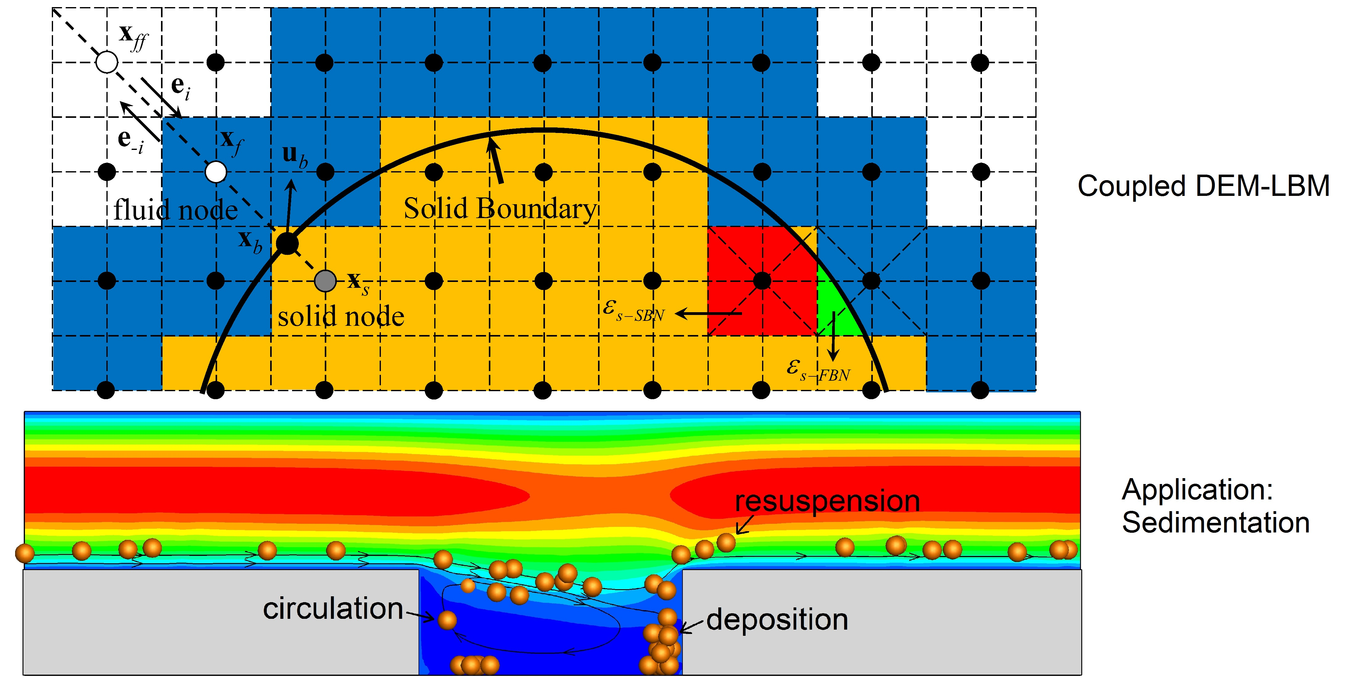
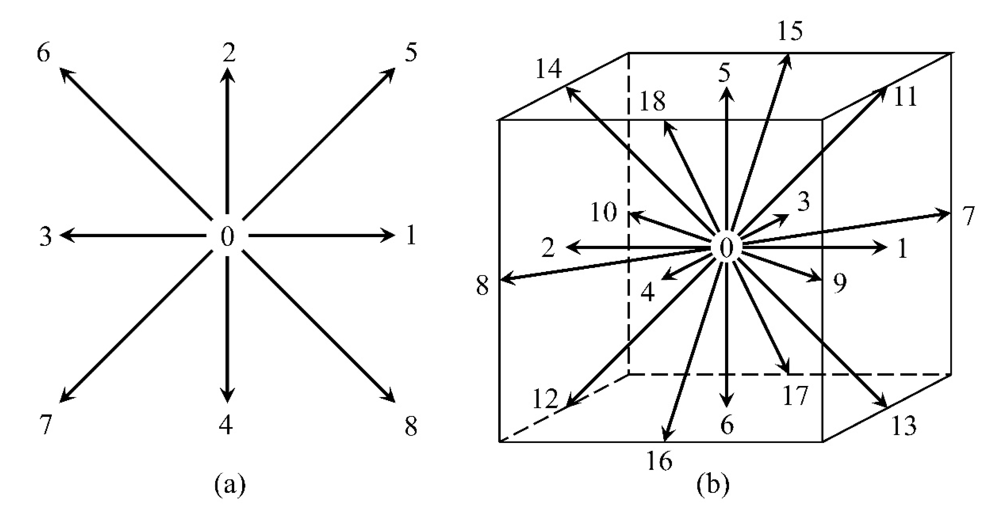
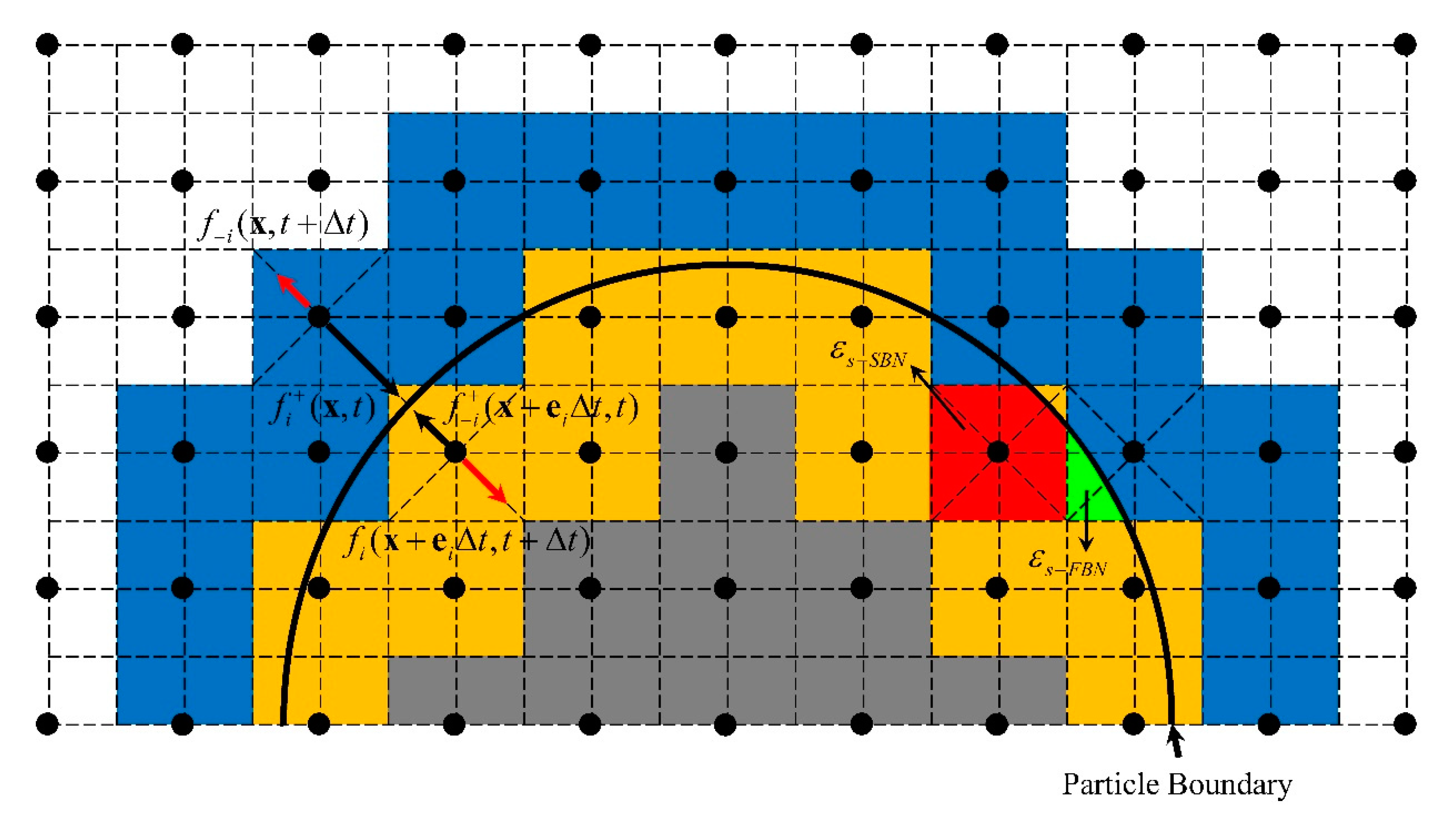
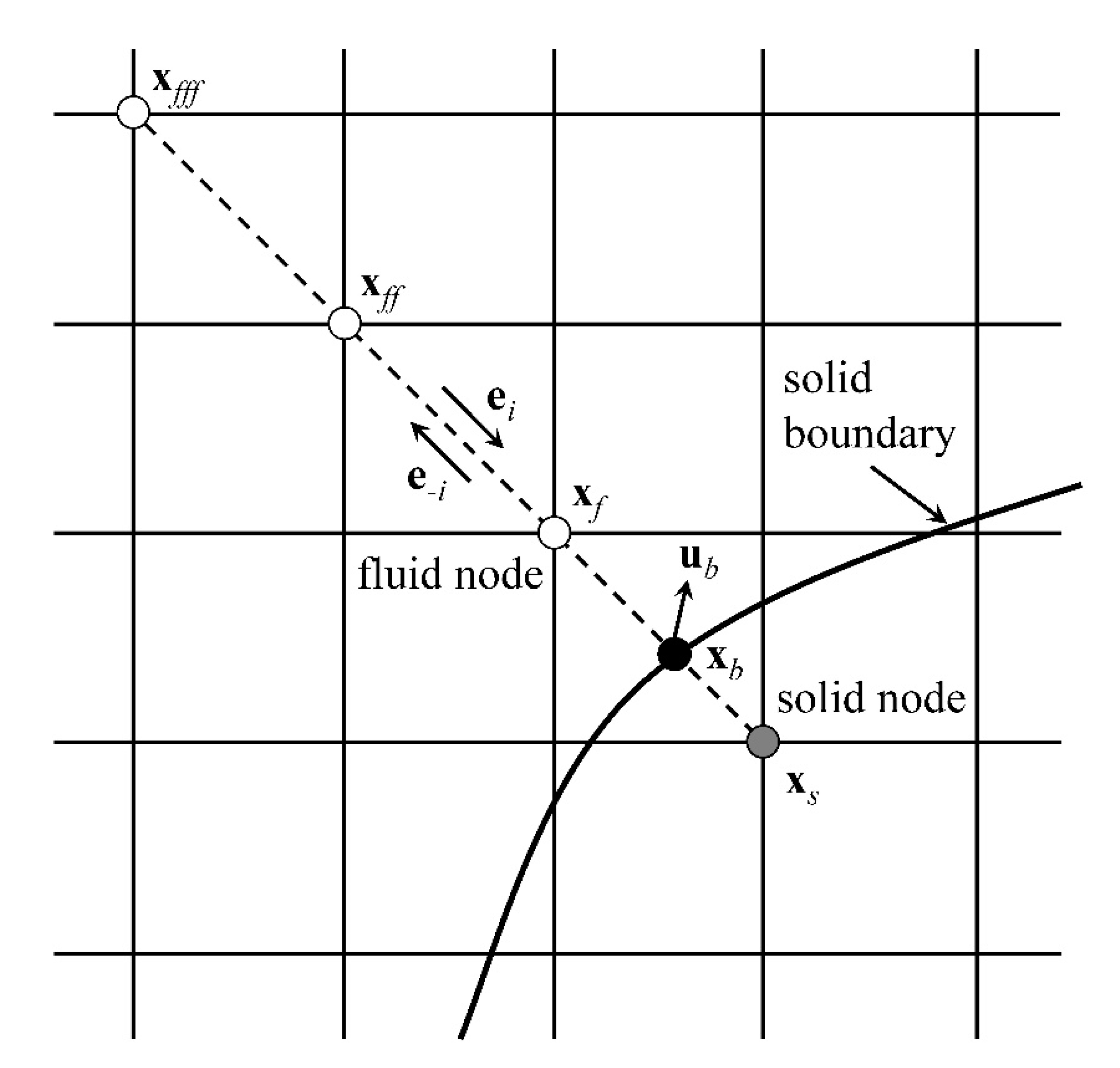
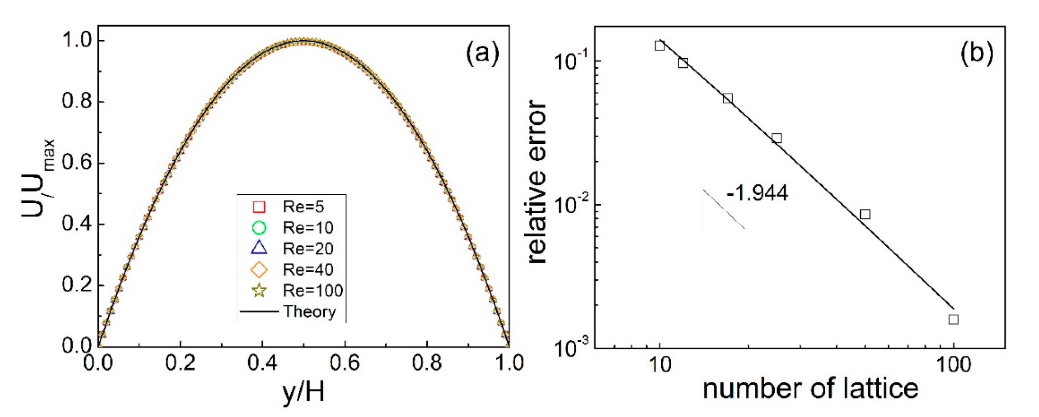
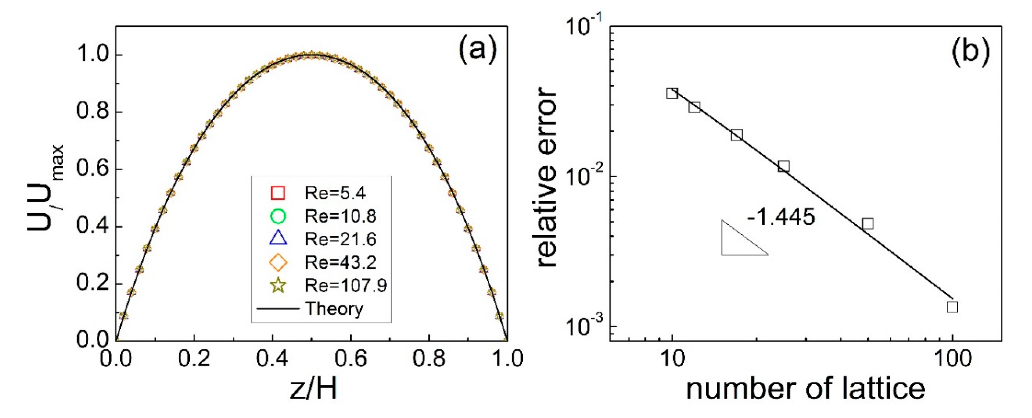
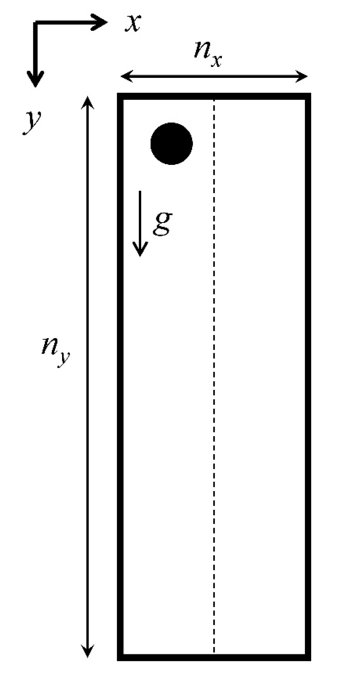
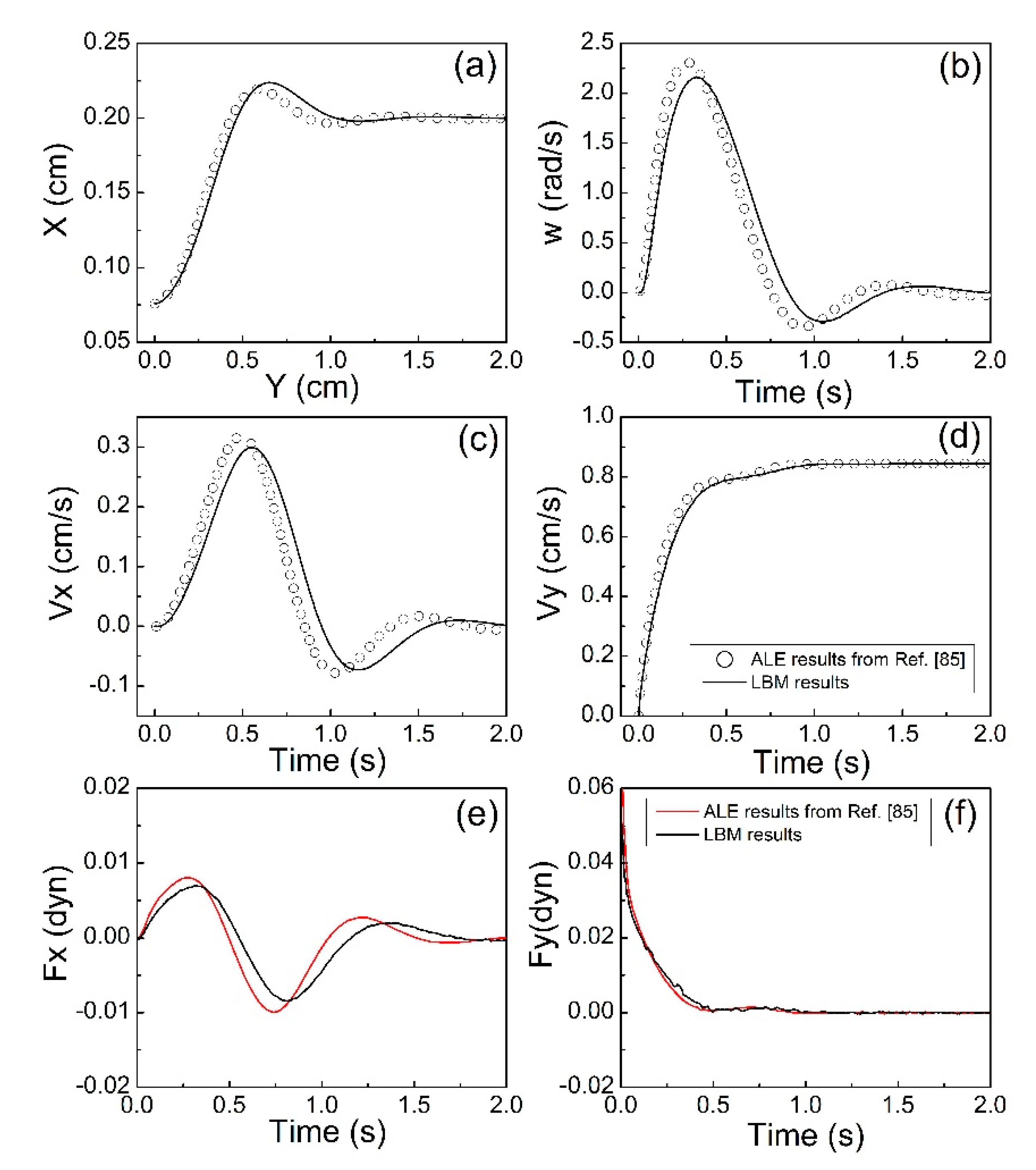
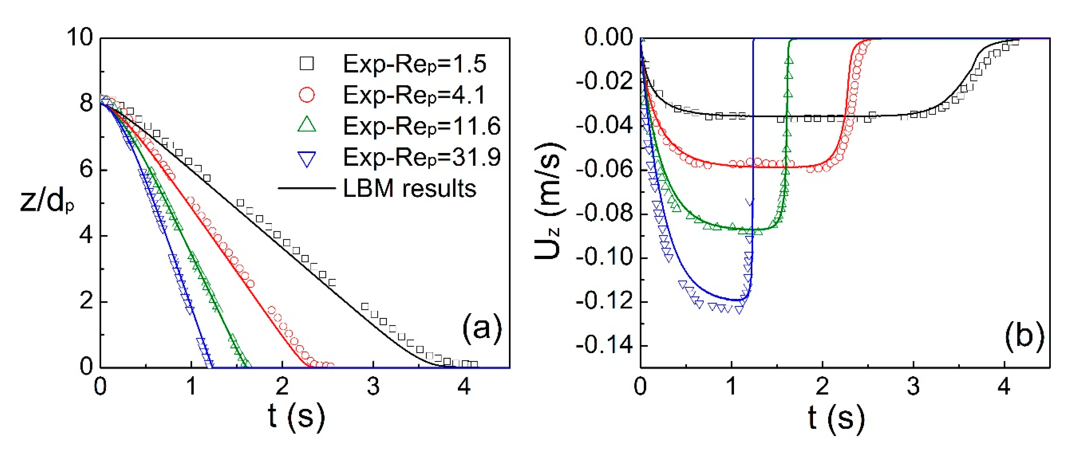
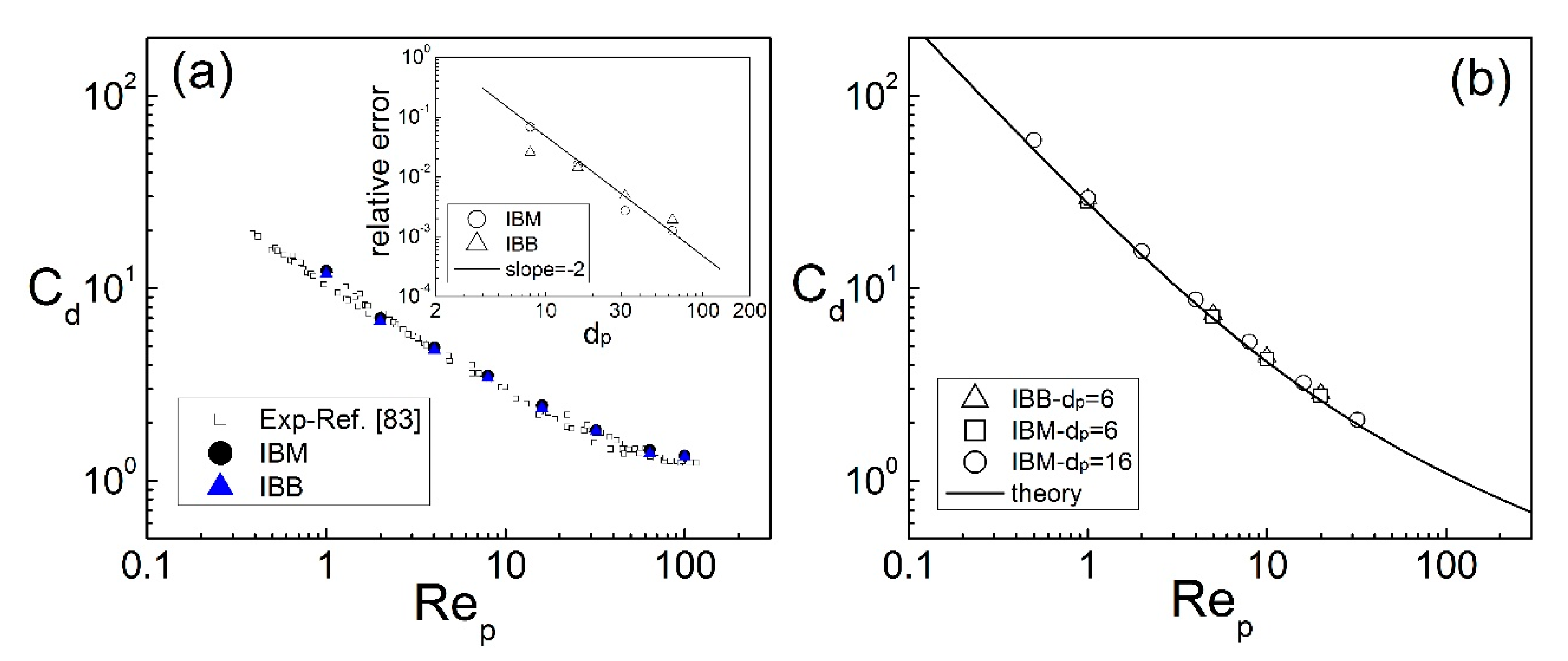
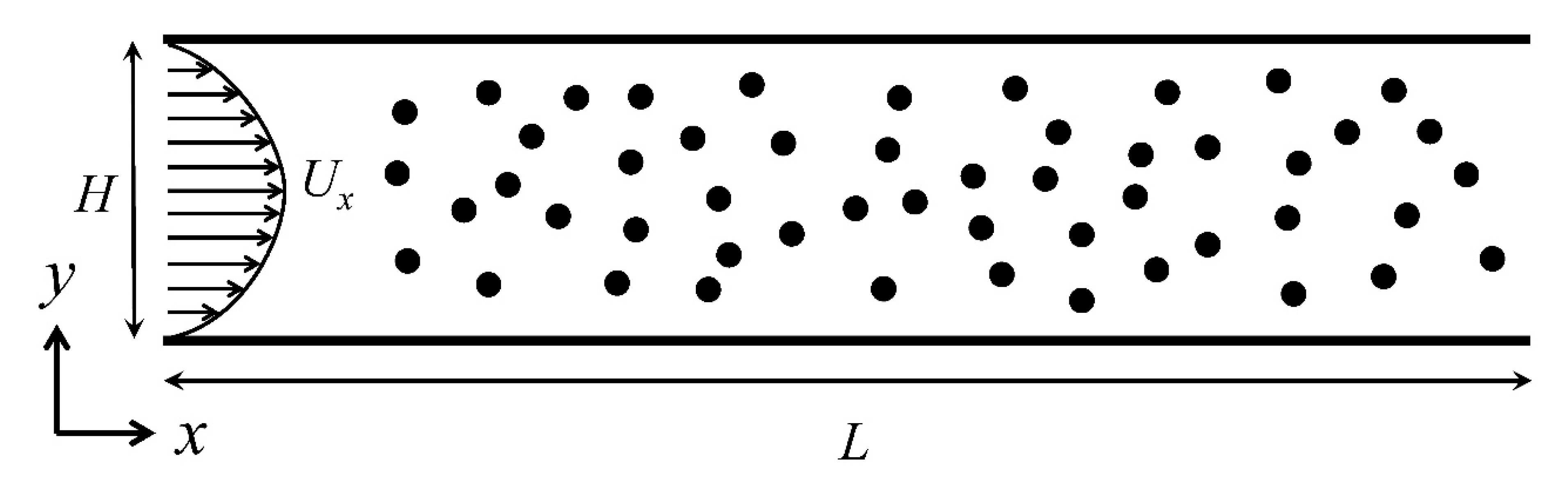
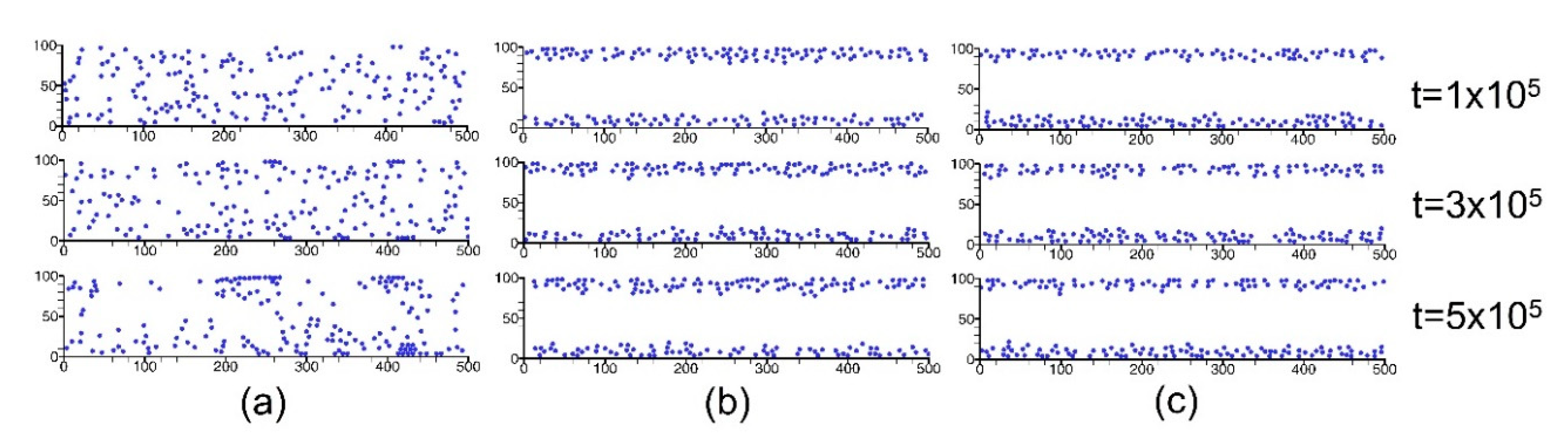
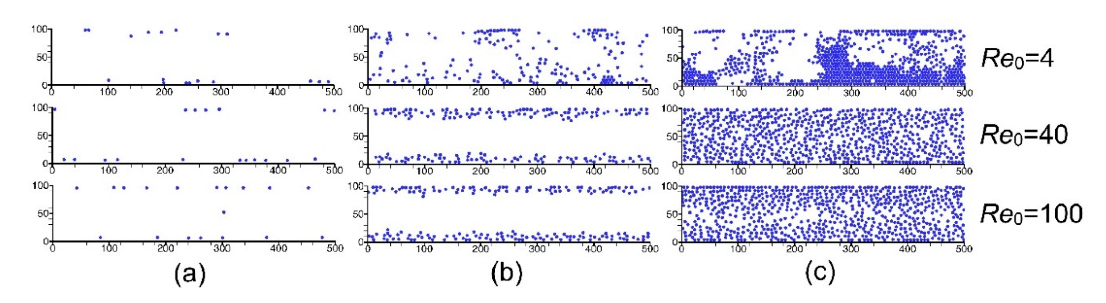
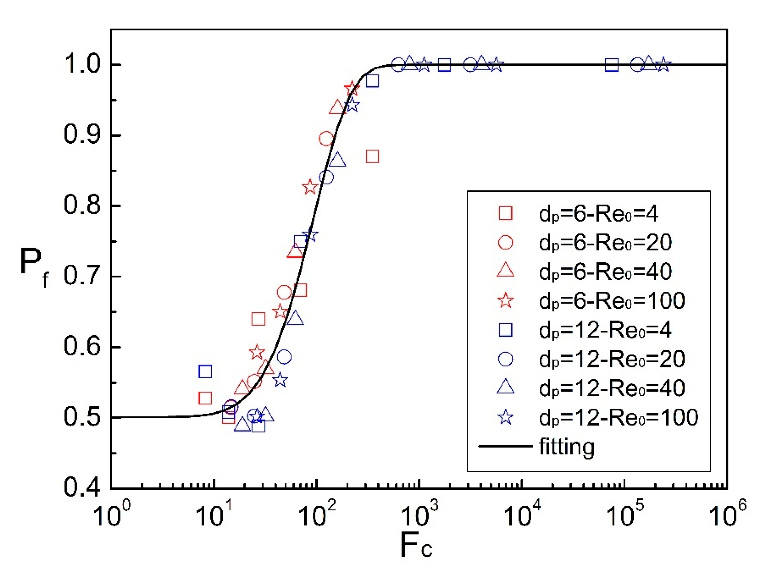
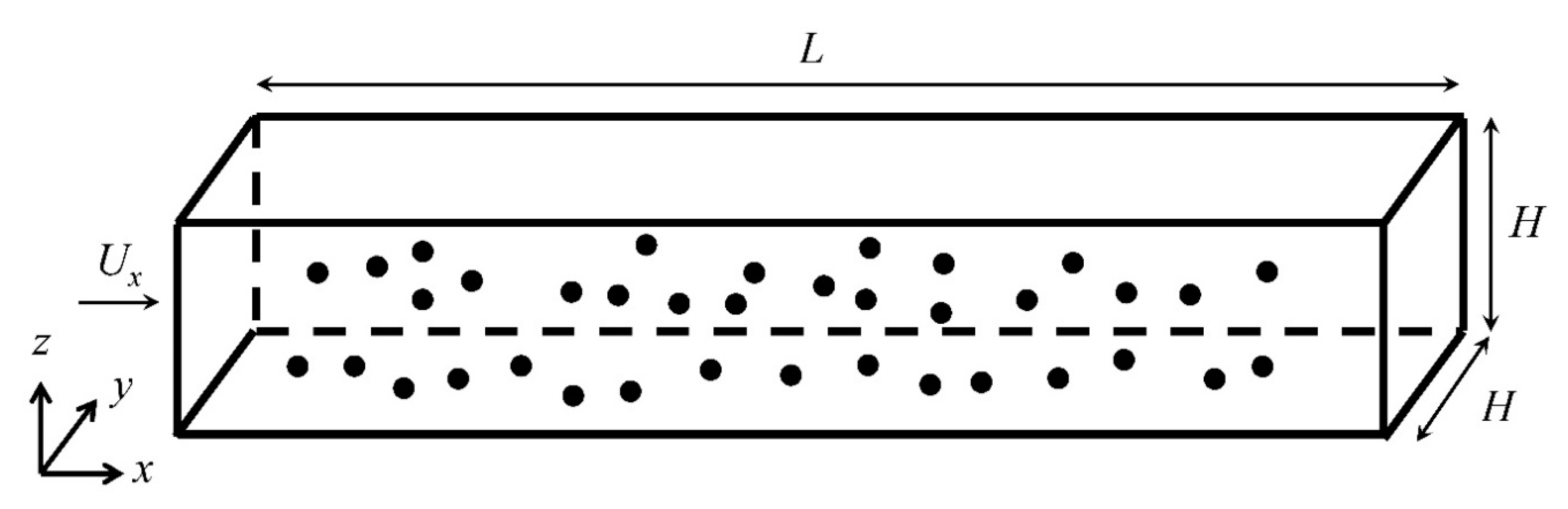
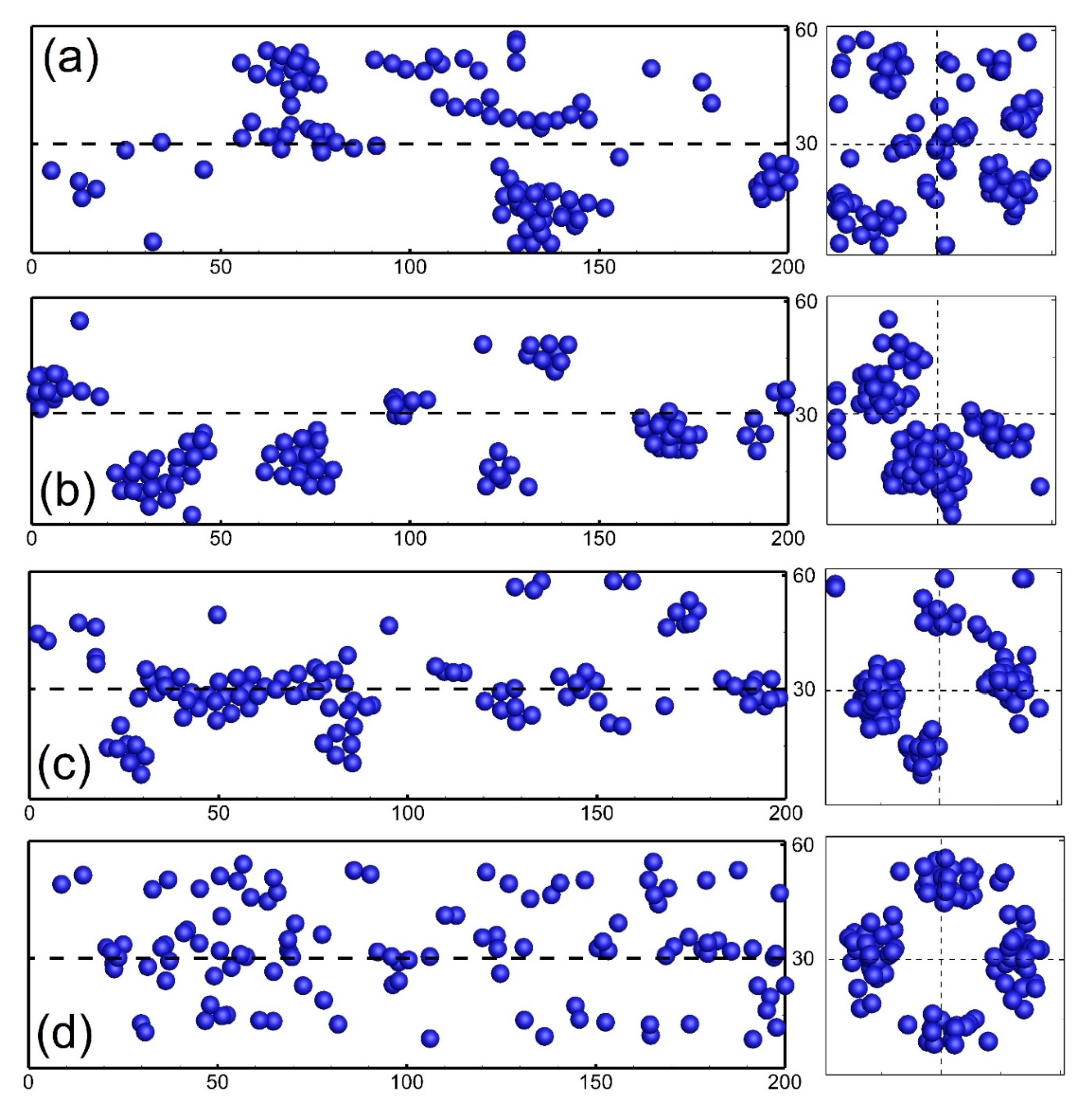
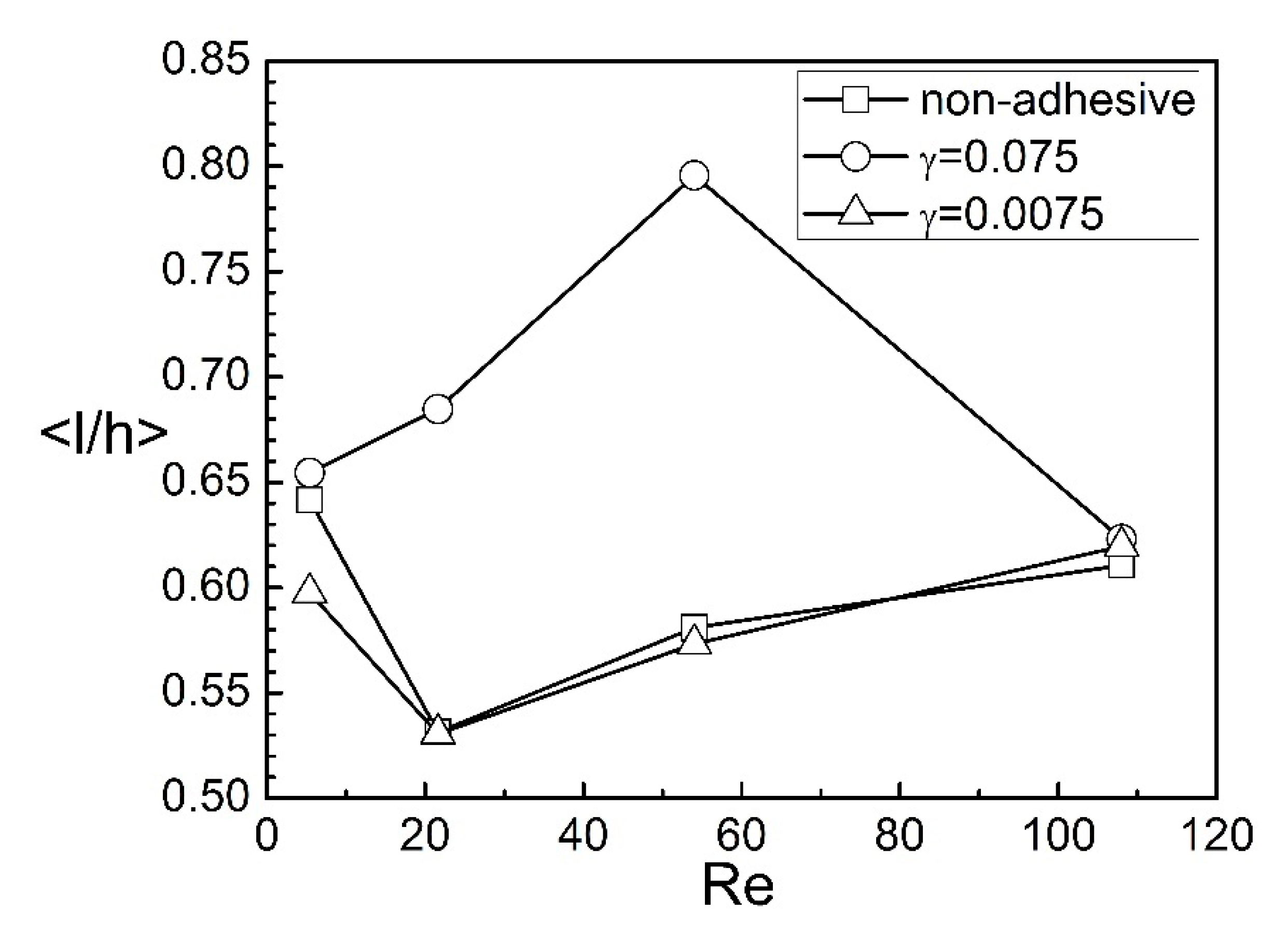
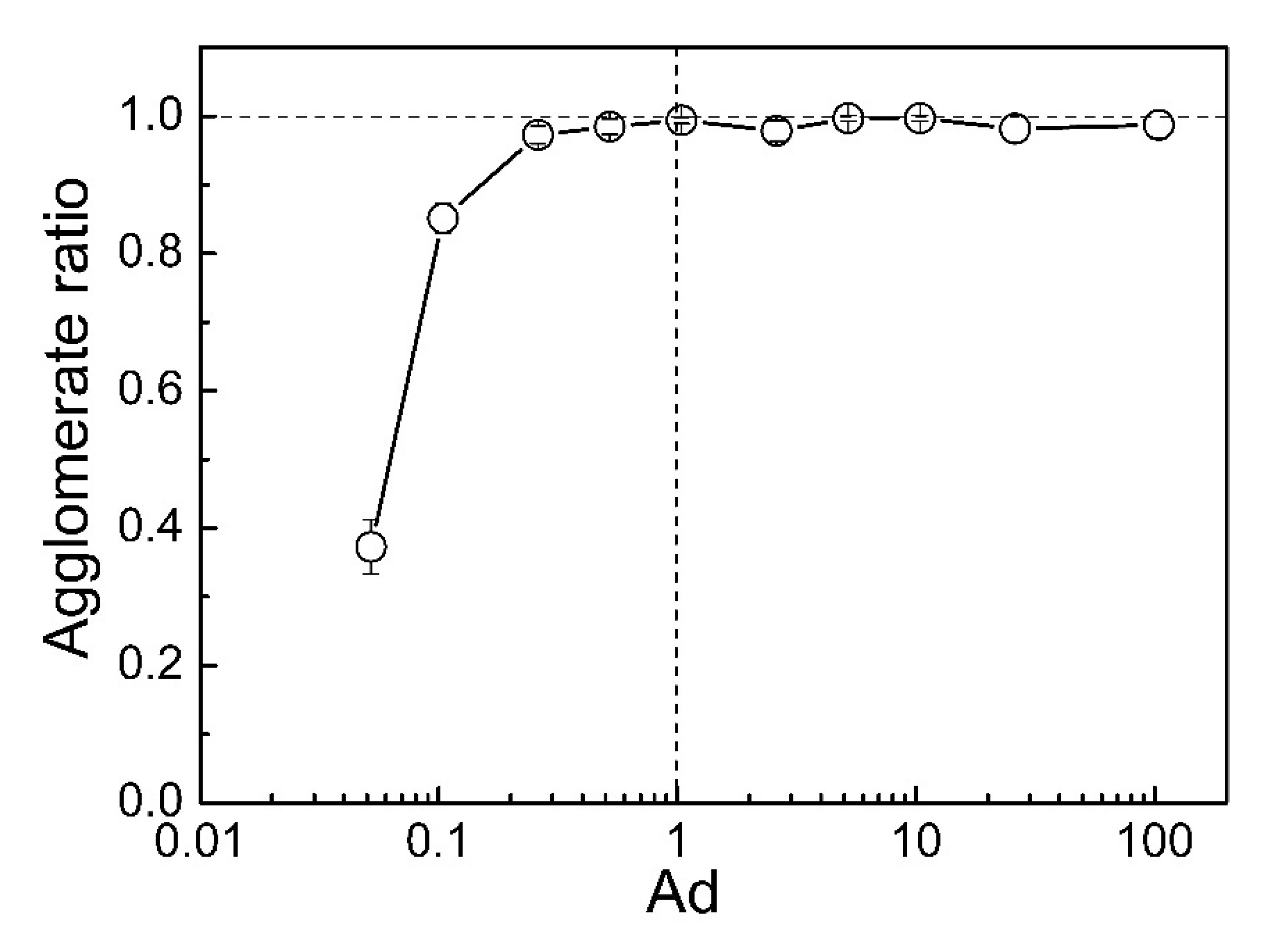
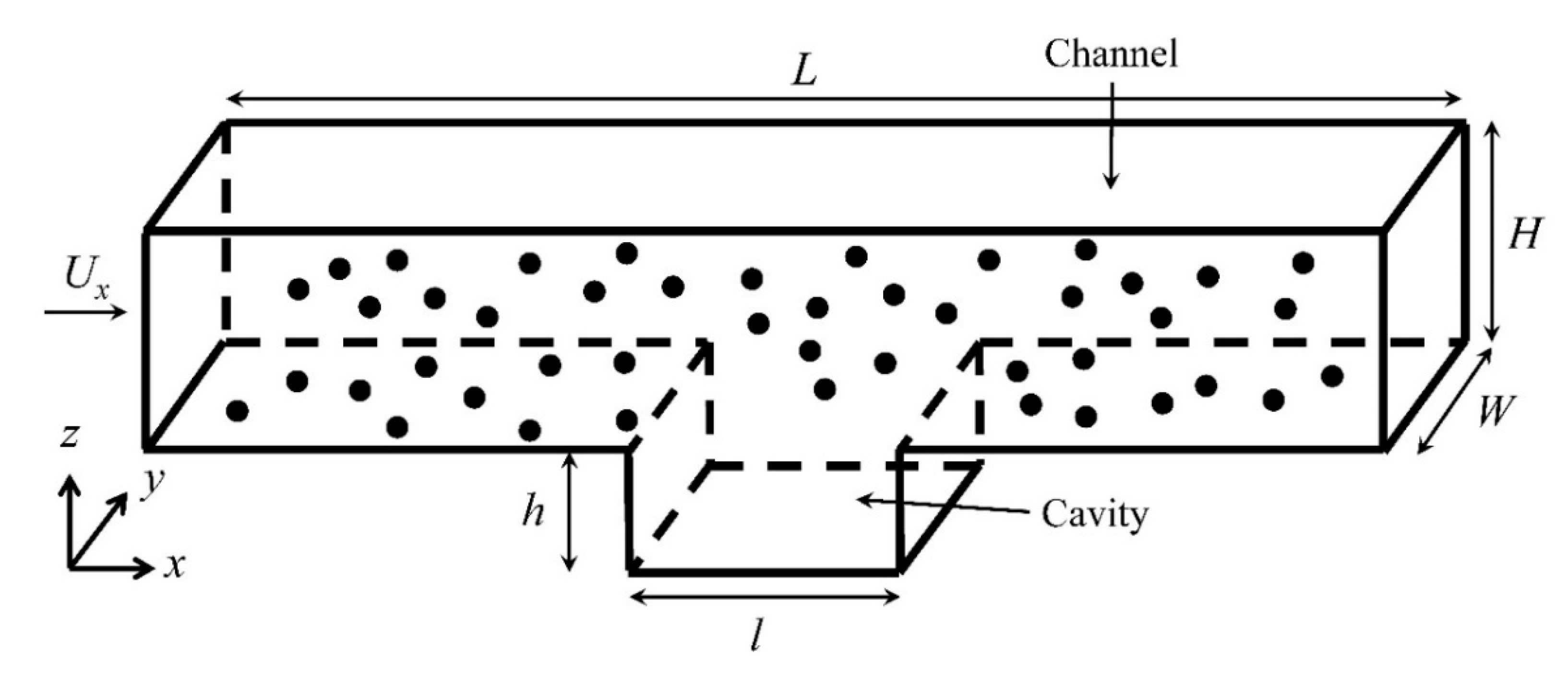
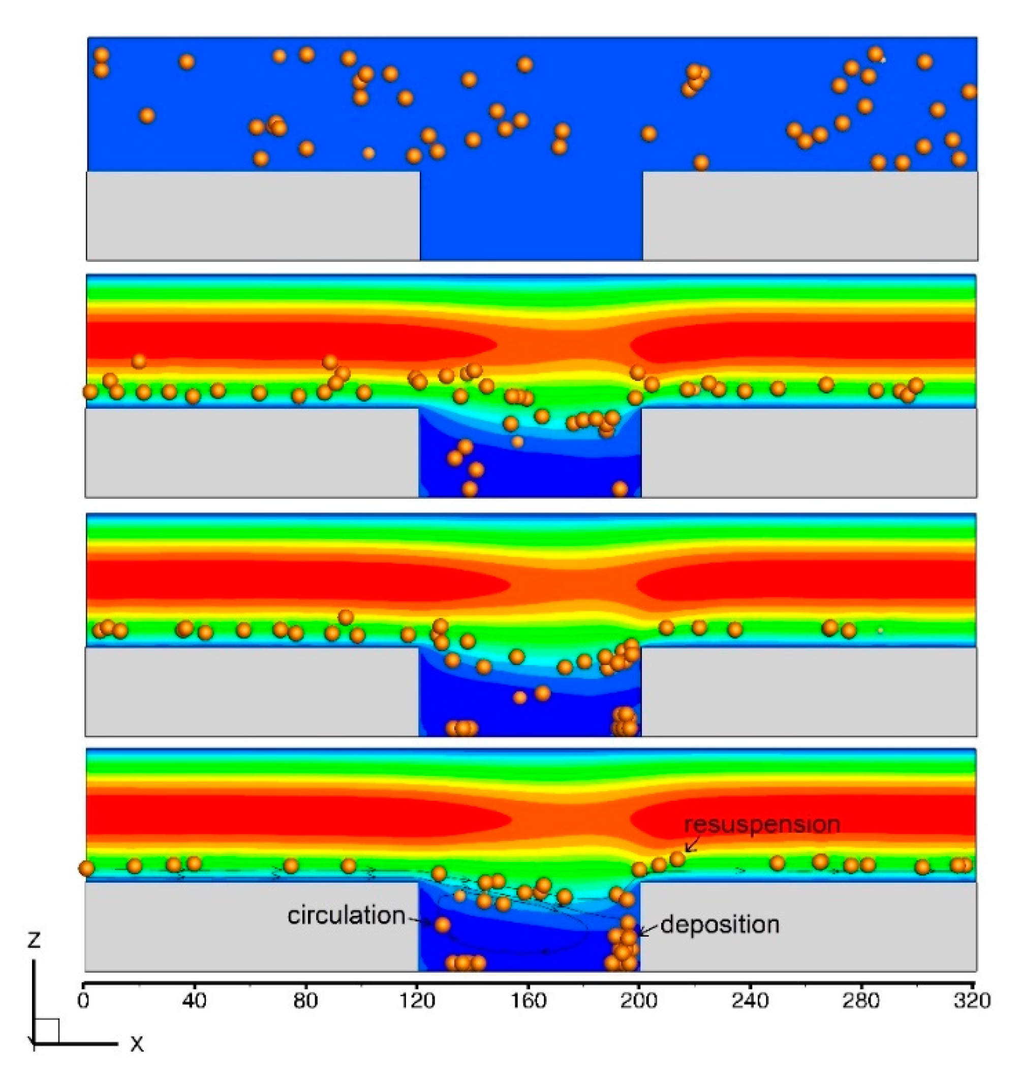
Table 1.
Unit conversion of 3D pipe flow.
| Physical Parameters | Unit | Real Value | Lattice Value | Conversion Coefficient |
|---|---|---|---|---|
| Pipe length (L) | m | 0.008 | 100 | 8.0 × 10⁻⁵ |
| Pipe diameter (D) | m | 0.004 | 50 | 8.0 × 10⁻⁵ |
| Fluid density (ρf) | kg/m3 | 1000 | 1 | 1000 |
| Fluid kinematic viscosity (νf) | m2/s | 1.0 × 10⁻⁶ | 0.05 | 2.0 × 10⁻⁵ |
| Average fluid velocity (V) | m/s | 0.0125 | 0.05 | 0.025 |
| Pressure drop (ΔP) | Pa | 0.2 | 3.2 × 10⁻³ | 62.5 |
| Time step (Δt) | s | 3.2 × 10⁻⁴ | 1 | 3.2 × 10⁻⁴ |
© 2020 by the authors. Licensee MDPI, Basel, Switzerland. This article is an open access article distributed under the terms and conditions of the Creative Commons Attribution (CC BY) license (http://creativecommons.org/licenses/by/4.0/).
Share and Cite
MDPI and ACS Style
Liu, W.; Wu, C.-Y. Modelling Complex Particle–Fluid Flow with a Discrete Element Method Coupled with Lattice Boltzmann Methods (DEM-LBM). ChemEngineering 2020, 4, 55. https://0-doi-org.brum.beds.ac.uk/10.3390/chemengineering4040055
AMA Style
Liu W, Wu C-Y. Modelling Complex Particle–Fluid Flow with a Discrete Element Method Coupled with Lattice Boltzmann Methods (DEM-LBM). ChemEngineering. 2020; 4(4):55. https://0-doi-org.brum.beds.ac.uk/10.3390/chemengineering4040055
Chicago/Turabian StyleLiu, Wenwei, and Chuan-Yu Wu. 2020. "Modelling Complex Particle–Fluid Flow with a Discrete Element Method Coupled with Lattice Boltzmann Methods (DEM-LBM)" ChemEngineering 4, no. 4: 55. https://0-doi-org.brum.beds.ac.uk/10.3390/chemengineering4040055