
Thermodynamic Design of Organic Rankine Cycle (ORC) Based on Petroleum Coke Combustion


Tomer Ltd., Tel-Aviv 6473424, Israel
ChemEngineering 2021, 5(3), 37; https://0-doi-org.brum.beds.ac.uk/10.3390/chemengineering5030037
Submission received: 29 May 2021
/
Revised: 10 July 2021
/
Accepted: 14 July 2021
/
Published: 16 July 2021
(This article belongs to the Special Issue Green Chemistry Technologies: Sustainable Approach to Chemical Engineering)
Abstract
:Thermodynamic analysis of Organic Rankine Cycle (ORC) was performed in this work. The Petroleum Coke burner provided the required heat flux for the Butane Boiler. The simulation of pet-coke combustion was carried out by using Fire Dynamics Simulator software (FDS) version 5.0. Validation of the FDS calculation results was carried out by comparing the temperature of the gaseous mixture and CO2 mole fractions to the literature. It was discovered that they are similar to those reported in the literature. An Artificial Intelligence (AI) time forecasting analysis was performed on this work. The AI algorithm was applied to the temperature and soot sensor readings. Two Python libraries were applied in order to forecast the time behaviour of the thermocouple readings: Statistical model—ARIMA (Auto-Regressive Integrated Moving Average) and KERAS—deep learning library. ARIMA is a class of model that captures a suite of different standard temporal structures in time series data. Keras is a python library applied for deep learning and runs on top of Tensor-Flow. It has been developed in order to perform deep learning models as fast and easily as possible for research and development. The model accuracy and model loss plot shows comparable performance (train and test). Butane has been employed as a working fluid in the ORC. Butane is considered one of the best pure fluids in terms of exergy efficiency. It has low specific radiative forcing (RF) compared to Ethane and Propane. Moreover, it has zero ozone depletion potential and low Global Warming Potential. It is considered flammable, highly stable and non-corrosive. The thermodynamic properties of Butane needed to evaluate the heat rate and the power were calculated by applying the ASIMPTOTE online thermodynamic calculator. It was shown that the calculated net power of the ORC cycle is similar to the net power reported in the literature (relative error of 4.8%). The proposed ORC energetic system obeys the first and second laws of thermodynamics. The thermal efficiency of the cycle is 20.4%.
1. Introduction
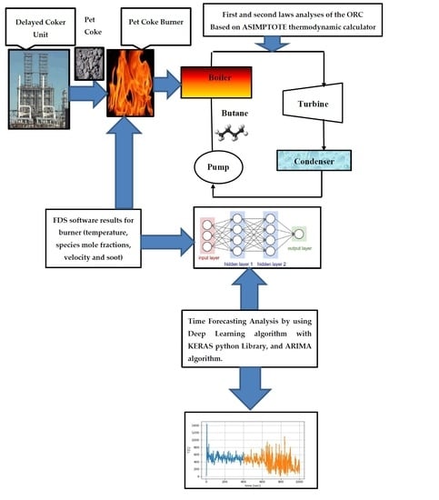
Pet-coke (Petroleum Coke) is a heavy crude oil refining coproduct. It is identified as a black-colored and carbon-rich solid. Despite the few human health or environmental risks posed by the exploitation of pet-coke, it has many industrial applications. It is mostly applied as a boiling and combusting fuel in industrial, power generation, and cement plants. Pet-coke is considered a promising substitute for steam coal in power plants because of its higher heating value, carbon content, and low ash, compared to bituminous coals. However, pet-coke gasification is a difficult process because of its high content of fixed carbon and low volatile matter [1]. The pet-coke generated by delayed cokers has great advantages such as high heating value (over 8500 kcal/kg). This is due to the fact it contains high carbon content (75–80% by weight) and low ash content (under 1%) [2]. The coke yield is about 33% [3]. It should be noted that coke burns also in FCC regenerators. The coke-coated catalysts are burned inside the FCC regenerators in order to restore catalytic activity and to provide the required heat flux for the cracking reactions taking place inside the FCC risers [4]. Computational Fluid Dynamics (CFD) is applied for predicting the hydrodynamic properties and other characteristics of fluidized beds and chemical reactors [5]. Several works have been written about pet-coke combustion applications in Energy production. Hamadeh et al. [6] have carried out a techno-economic analysis of an oxy-pet-coke plant with carbon dioxide capture simulated at pressures between 1 and 15 bars in Aspen PlusTM. Shen et al. [7] have carried out a feasibility economic study. Their study included two main systems: The first Integrated Gasification Combine Cycle (IGCC) complex was applied. The syngas mixture generated by IGCC was burned in the Heat Recovery Steam Generator (HRSG). The second system offered the earliest opportunity for the commercial production of Coal to Liquids (CTL) fuels. The production of liquid fuel was carried out by employing Fischer–Tropsch (F-T) process. The aim of this research is to investigate whether the pet-coke burner can provide the necessary heat flux for the Organic Rankine Cycle (ORC) normal operation. This paper presents a new detailed design of ORC based on a pet-coke burner. The algorithm is composed of CFD modelling of hydrodynamics, heat transfer, and pet-coke combustion. Based on the CFD results, the Time Forecasting Modelling Behavior of pet-coke combustion was applied by using Artificial Intelligence (AI) Algorithms. Thermodynamic analysis was carried out on the ORC. It was found that the pet-coke particles are mostly applied in the Heat Recovery Steam Generator (HRSG), in Integrated Gasification Combine Cycle (IGCC) [7], in Circulating Fluidized Bed (CFB) power plants [2], or in Rotary Kilns (see Section 2.2). To the best of my knowledge, it is probably the first time that a small-scale pet coke box burner has been implemented as a heat source for operating Organic Rankine Cycle with Butane working fluid. There are several applications pet-coke ORC Power systems. For example, the ORC power plant can be close to the refinery where the refinery uses its electric power. Green Hydrogen required for Hydrocracking and Hydrodesulphurization (HDS) reactions may be produced by water splitting. This system may be also applied for a backup solar power cycle. As far as I know, this work is the first coupled CFD simulation of pet-coke burner with ARIMA and Deep learning algorithms and ASIMPTOTE online thermodynamic calculator. This system is shown in Figure 1.
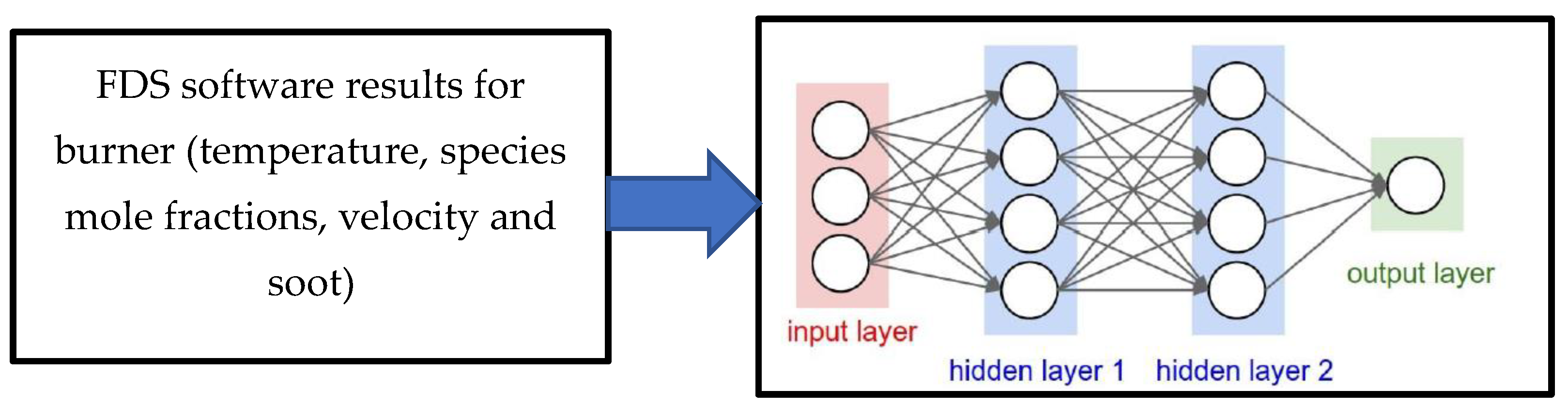
The simulation pet-coke burner is described at the bottom of Figure 1. An Artificial Intelligence (AI) time forecasting algorithm was applied on the pet-coke burner.
Review of the Applications of Deep Learning Analysis of Combustion
Multilayer Perceptions (or artificial neural networks—ANN) are constructed from a collection of interconnected nodes, and input and output layers. Inputs are weighted results provided by the input layer. Each perceptron also has a hidden layer. The perceptron forms a linear equation that relates the inputs and the hidden layer to the output. An activation function is employed in the output so that the system can learn nonlinear relationships. Common activation functions include a sigmoid, step function, rectified linear unit (RELU), or hyperbolic tangent. The Combination of the entire network results in a series of linear equations [8].
Deep learning algorithms have recently predicted full-field fire conditions in building fires (gas temperatures, velocities) and wildland fires [9]. Deep learning had been developed using convolutional neural networks (CNN) in order to study the flux dependence from CFD model training data. A comprehensive data-driven approach has developed in order to predict spatially resolved temperatures and velocities within a compartment based on coarse zone fire modeling by using a transpose convolutional neural network (TCNN) [9]. A thousand Fire Dynamics simulations (FDS) of a simple two-compartment configuration with different fire locations, fire sizes, ventilation configurations, and compartment geometries were applied for training and testing the model. The TCNN approach was also validated with two more complex multi-compartment FDS simulations by processing each room individually. Sun et al. [10] have developed three feed-forward neural network (FFNN) models with the backpropagation by applying Levenberg−Marquardt algorithm. These three models were designed for jet fire, early pool fire, and late pool fire accident scenarios.
2. Materials and Methods
2.1. Fire Dynamic Simulation (FDS) Modeling of the Pet-Coke Burner
This software was developed at the National Institutes of Standards and Technology (NIST) [11,12,13]. It solves simultaneously the momentum, energy and diffusion transport equations. In addition to that, it also solves the equation of state within each numerical grid cell as a function of time. It also provides the heat release rate (HRR). The “smoke-view” postprocessor software was applied in order to simulate the pet-coke burner combustion performance. The components and Governing Equations of FDS Software are described in detail in [14].
2.2. FDS Modelling of the Combustor
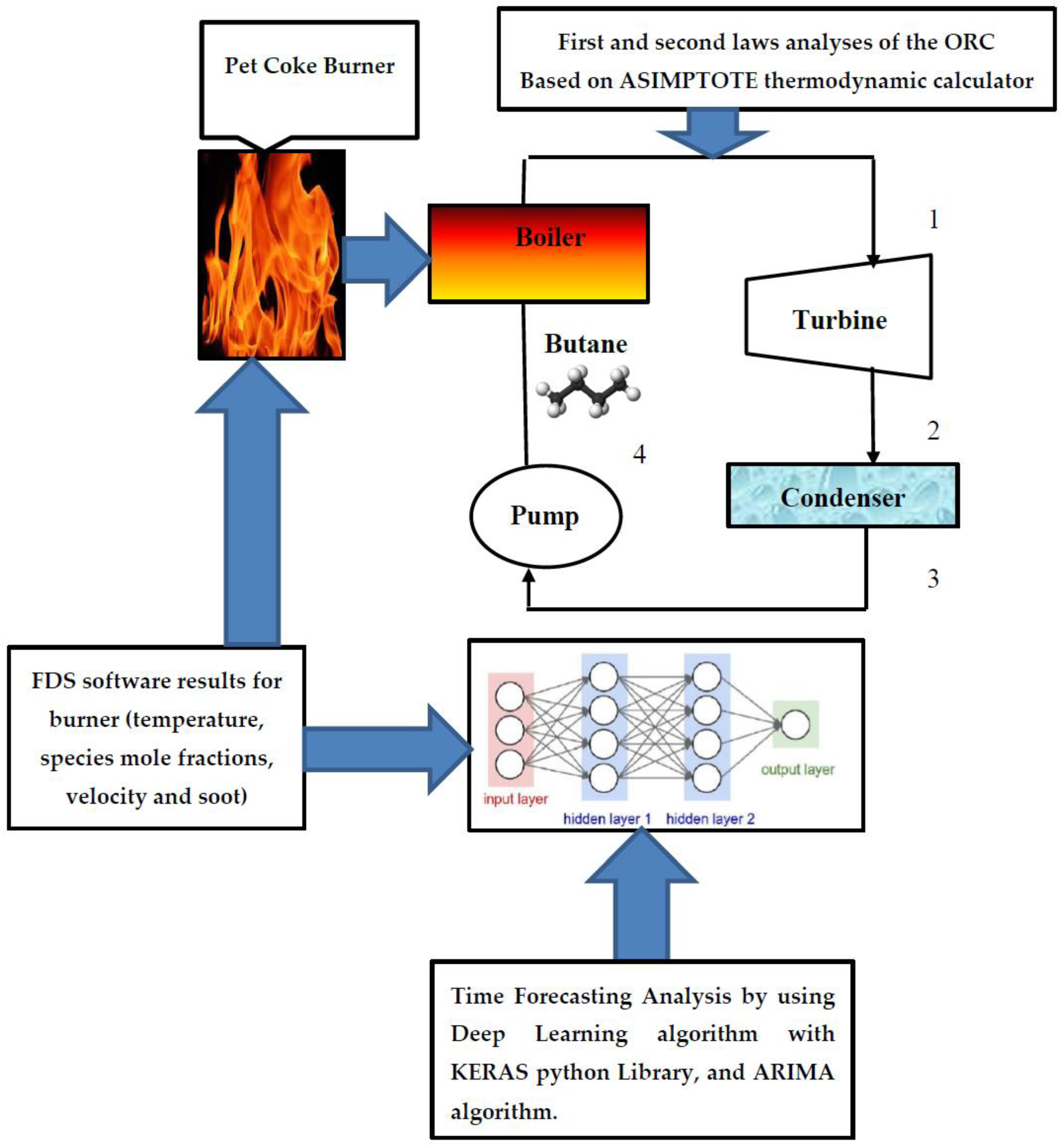
The geometrical model of the pet-coke burner is shown in Figure 2.
The height, length and width of the burner are 4.0 m, 2.0 m and 3.0 m, respectively. It contains 24,000 cells. Coke particles are injected and ignited at the bottom side of the burner. The numerical model of the pet-coke burner contains thermocouples and carbon dioxide concentration sensors. The sensors located at x = 4 m, y = 0 and at different heights z = 0.5 m, 1.0 m, 1.5 m, 2.0 m, 3.0 m, 3.5 m and 4.0 m (the coordinate system center is located at the center of the burner bottom plate—see Figure 2). The heat of combustion of the pet-coke is 38,379 (kJ/kg) [15].
Initial condition—it is assumed that the initial temperature, the component concentration in the air and pressure are:
Boundary Condition—it is assumed that all burner compartment walls are opened.
2.3. Time Forecasting Calculations by Applying Artificial Intelligence (AI) Algorithms
An Artificial Intelligence (AI) time forecasting analysis was performed in this section. This algorithm was applied to the temperature and carbon dioxide, carbon monoxide and soot sensors readings. Two Python libraries were employed in order to forecast the time behaviour of the thermocouple readings: Statistical model—ARIMA (Auto-Regressive Integrated Moving Average) and KERAS—Deep learning library. ARIMA [17] is a class of models that capture a suite of different standard temporal structures in time series data. Keras is a Python library for deep learning that runs on top of Tensor-Flow [18,19,20].
2.4. Thermodynamic Analysis of the Organic Rankine Cycle
It is assumed that the Steady State Steady Flow (SSSF) process. According to [21], the continuity equation is:
where represents the mass flow rate entering to the control volume (such as Heat Exchanger, Turbine, Condenser and Pump) in [kg/s], is the mass flow rate leaving the control volume in [kg/s]. the first law of thermodynamics for the SSSF process is [21]:
where is the heat indication rate invested/produced in the control volume (Heat Exchanger, Condenser) in [kW]. is the heat rate invested/Produced in the control volume in [kW]. is the enthalpy of the entering stream in [kJ/kg]. is the enthalpy of the leaving stream in [kJ/kg]. and are the velocity and height of the entering streams, respectively. and are the velocity and height of the streams leaving the control volume, respectively. The second law of thermodynamics for the SSSF process is [21]:
where is the entropy of the entering stream in [kJ/(kg K)]. is the entropy of the leaving stream in [kJ/(kg K)], is the time in [sec] and is the temperature in [K]. The Organic fluid, which flows inside the ORC cycle is Butane. The thermodynamic properties (such as enthalpy, specific volume) needed to evaluate the heat rate and the power were calculated by applying the ASIMPTOTE online calculator [22]. The Butane temperature at the outlet of the Boiler was calculated by applying an energy balance equation on the boiler:
where is the average of the Heat Release Rate in [kW].
2.5. Computation Structure Process of the Pet-Coke Burner
The simulation process algorithm discussed in the previous section is summarized in Figure 3. The algorithm is composed of four modules. FDS output file which contains the coke combustion simulation data.
3. Results
This section includes two parts. Section 3.1 presents the numerical results of Fire Dynamics Simulation (FDS) software. Section 3.2 presents the time forecasting analysis of the sensor readings by applying ARIMA and Deep learning algorithms (KERAS library).
3.1. Fire Dynamics Simulator Software Results for Burner
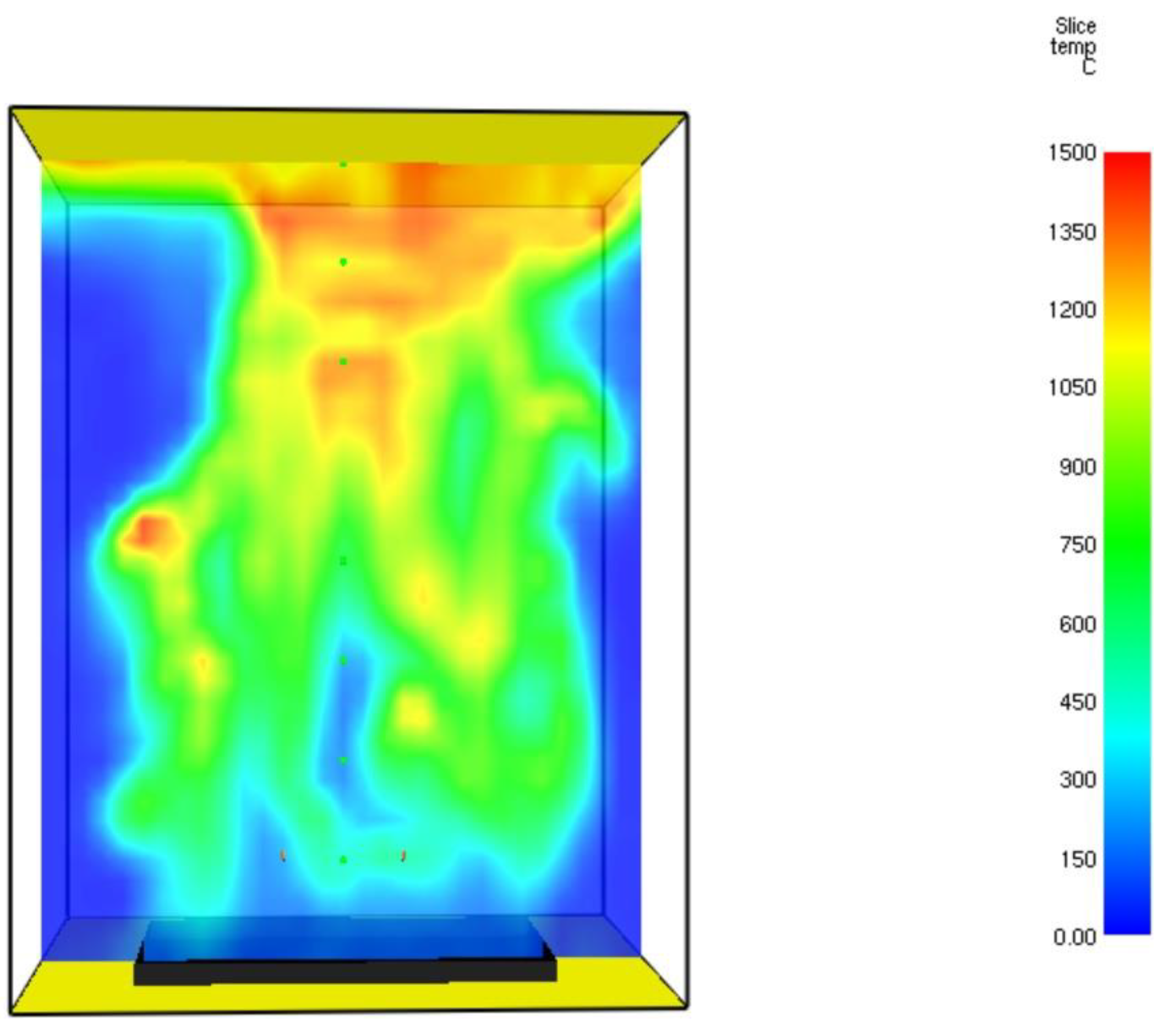
Figure 4 shows the temperature field of the pet-coke burner at t = 60.7 s.
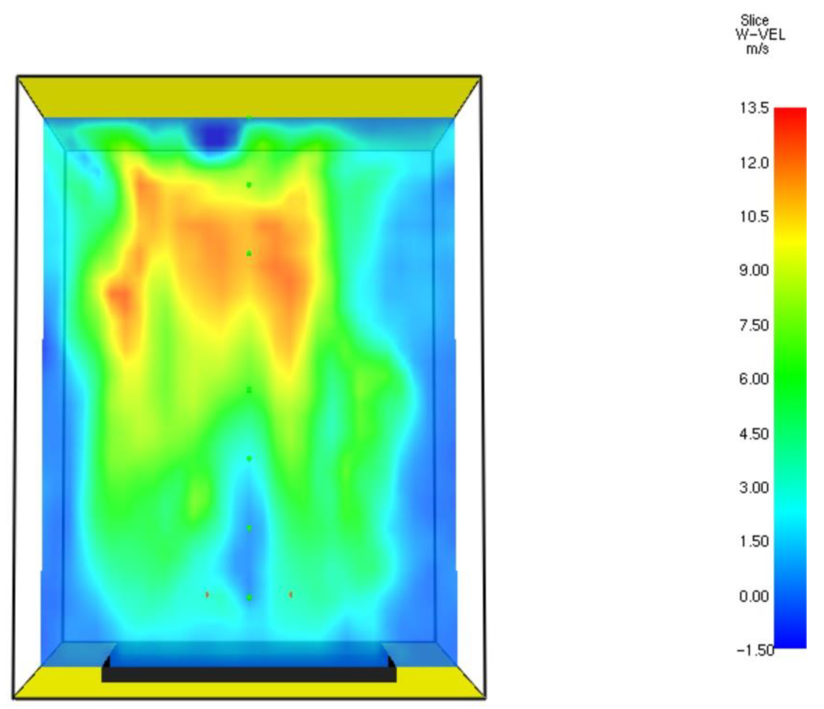
According to Figure 4, the maximal temperature reaches 1440 °C. A similar value was observed in [18]. The calculated temperature at the bottom region of the burner is about 700 °C. Similar to the temperature observed in [23]. Figure 5 shows the velocity field of flue gases at t = 60.7 s.
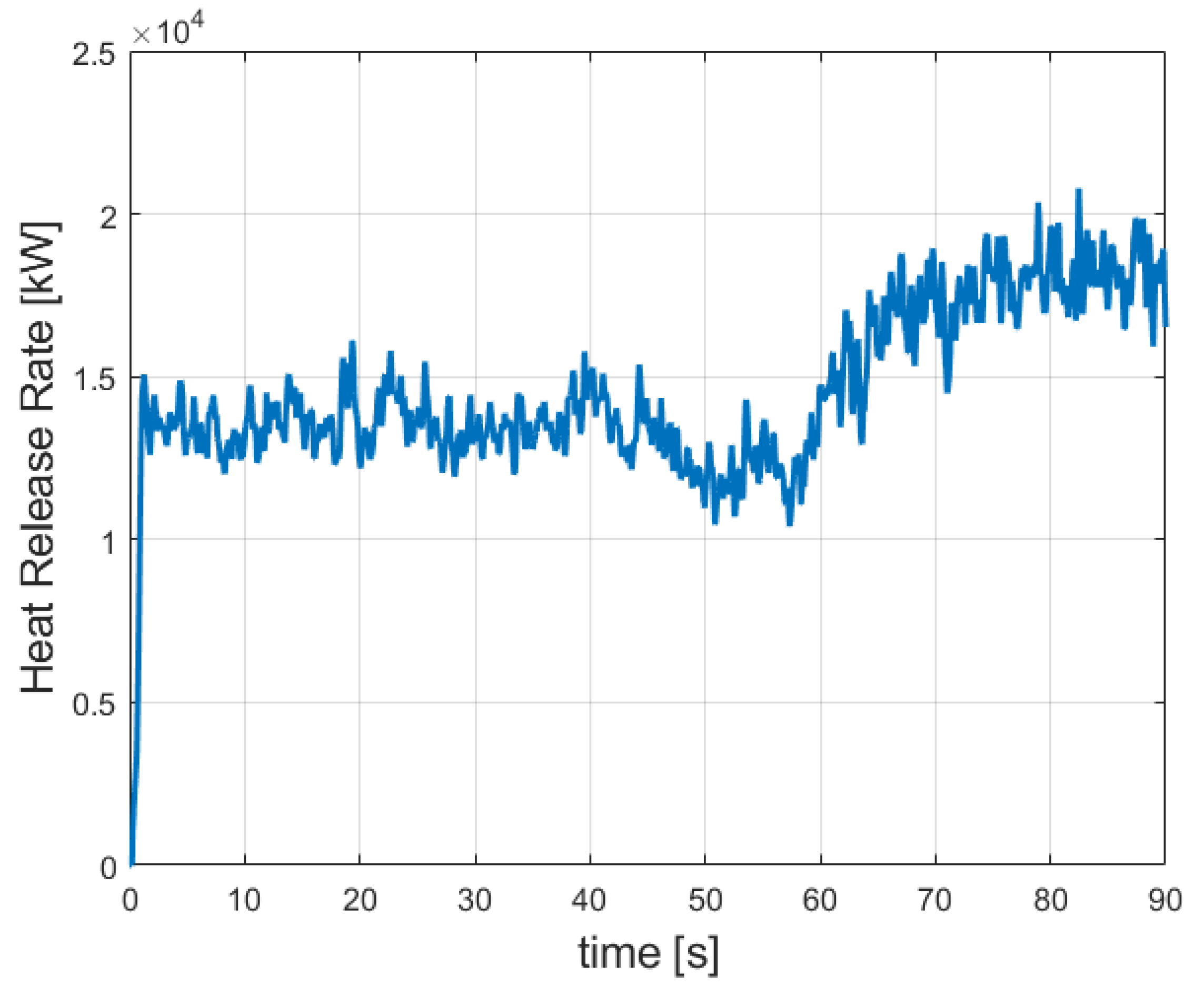
From Figure 5 it can be seen that the gaseous mixture flows upwards because of buoyancy forces. The velocity is higher near the ceiling. Based on the thermocouples and CO2 sensor readings, the following plots were constructed. Figure 6 shows the Heat Release Rate (HRR).
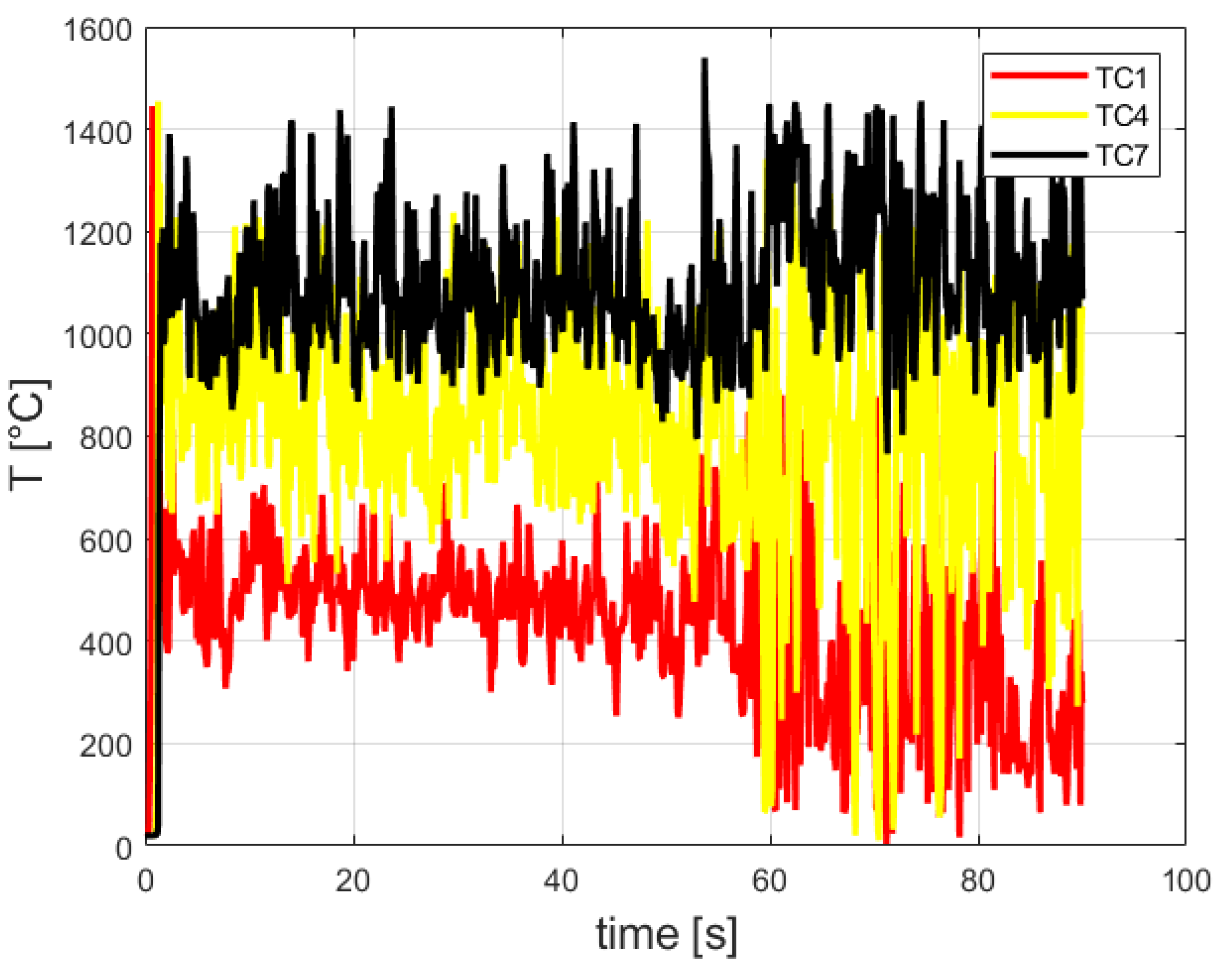
Figure 7 shows the temperature readings of TC1, TC4 and TC7 thermocouples.
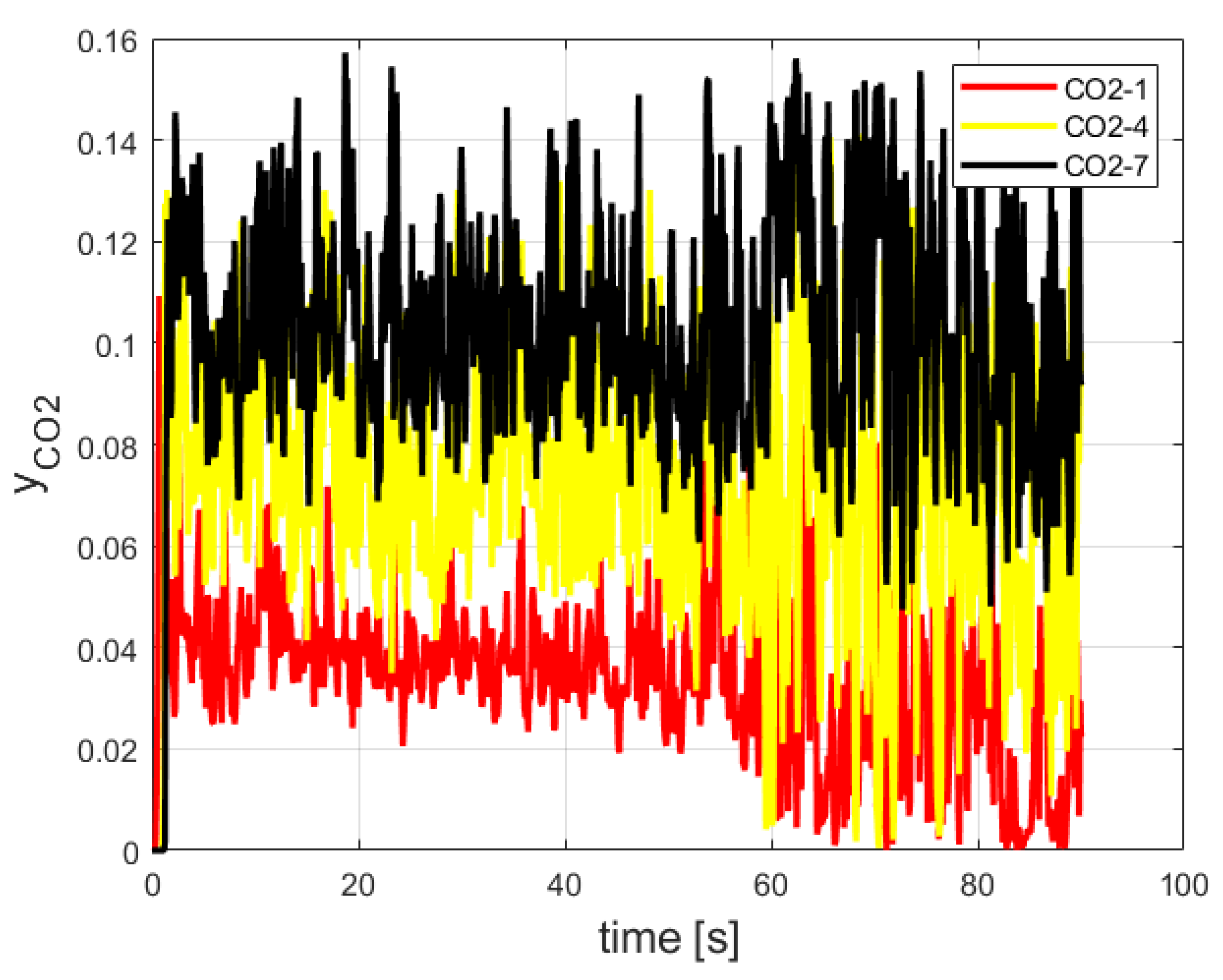
Figure 7 shows that the temperature readings of thermocouples TC4 and TC7 are much larger than the temperatures readings of TC1. This is due to the fact that buoyancy force causes the hot gas to flow towards the top of the burner. The maximal thermocouple reading is about: 1440 °C. It is similar to the temperature reported in [16]. Figure 8 shows the CO2 mole fraction readings of the three CO2 sensors.
As can be seen from Figure 8 the mole fraction readings are shown by CO2-4 and CO2-7 are much larger than CO2-1 sensor mole fraction readings. This is due to the fact that oxidation of the coke particles increases with the temperature. The maximal CO2-7 reading is 15.0%. The calculated carbon dioxide mole fraction is similar to those obtained in [24,25] which are 14.5% and 13.6%, respectively.
Grid Sensitivity Study Results
Verification of the CFD numerical results was carried out. Additional FDS models were developed containing 36,000 cells. The average temperature was computed by performing numerical integration of the instantaneous temperature readings over time (see Figure 7). The maximum difference is less than 7.5%.
3.2. Time Forecasting Analyses Results for the Calculated Temperature
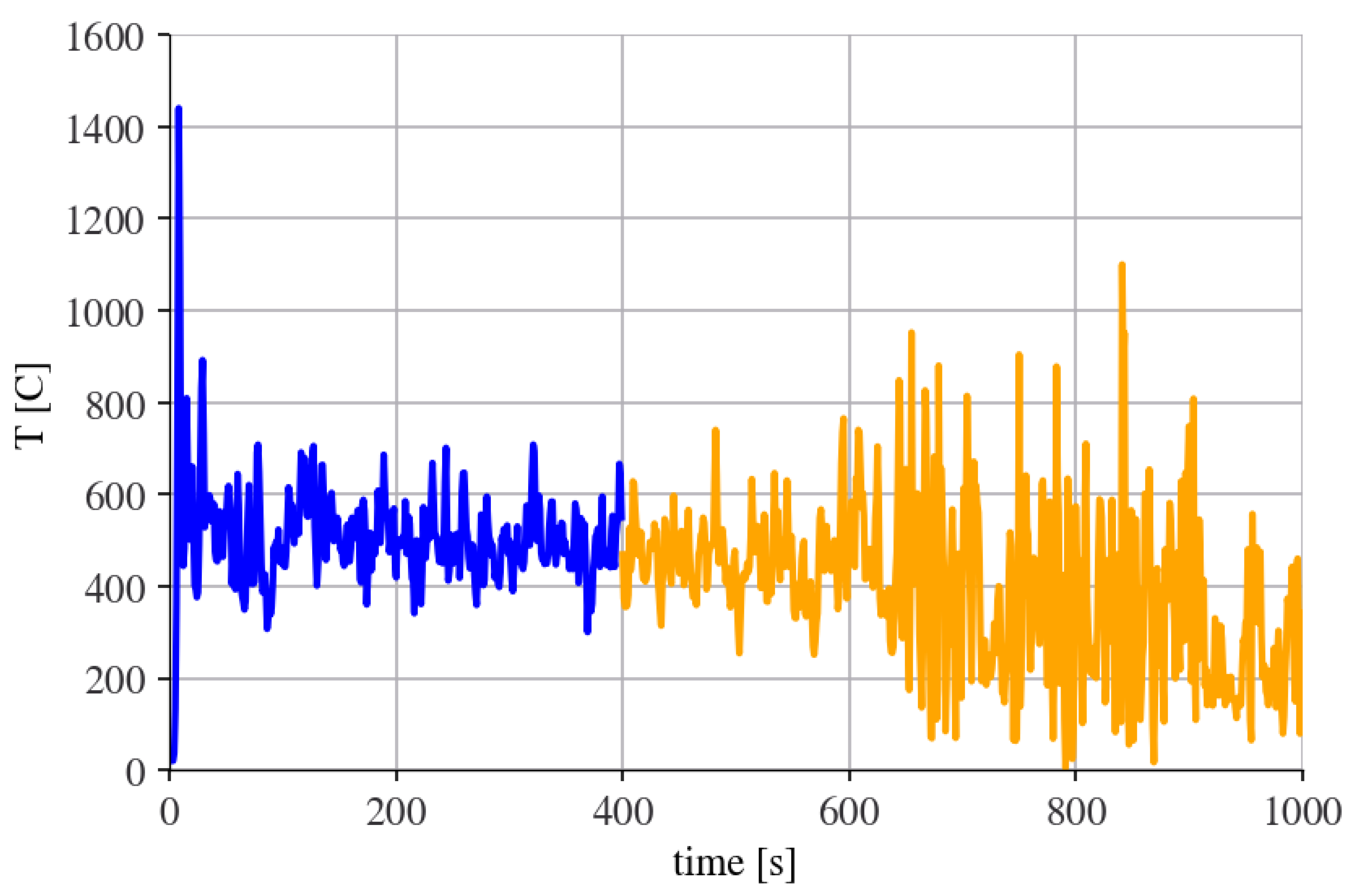
Time series forecasting problems are a difficult type of predictive modeling problem. A powerful type of neural network designed to handle this time sequence dependence. The time forecasting capabilities of Auto Regressive Integrated Moving Average (ARIMA) and CNN methods are employed in this work. Unlike the regression forecasting modeling, time series also adds the complexity of sequence dependence among the input variables. A graph was plot showing the expected values (blue) compared to the forecast predictions (orange).
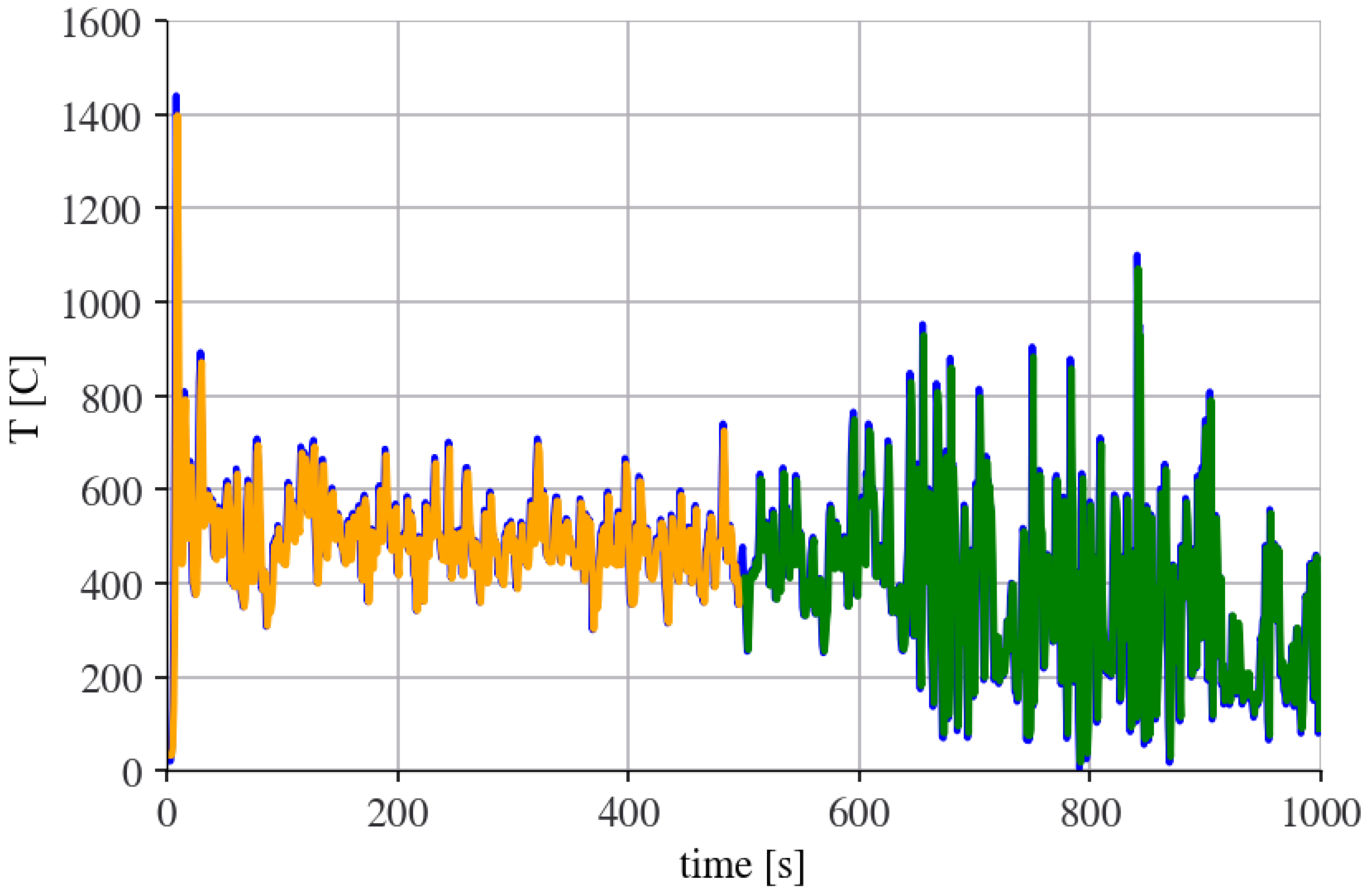
From Figure 9, it can be seen that the ARIMA model predicts very well the temperature reading of TC1 thermo-couple readings. The convolutional neural network (CNN) used in this work contains eight hidden layers. The RELU activation function was employed. This neural network was trained with several time-dependent CFD output files (including an additional FDS model which simulates Heptane burner). In all of them, the deep learning analysis proved that this CNN achieved excellent temperature predictions and provided a good theoretical verification of CNN for modelling pet-coke combustion. A graph was plot showing the expected values (blue) compared to the forecast predictions (orange) and the trained values (orange).
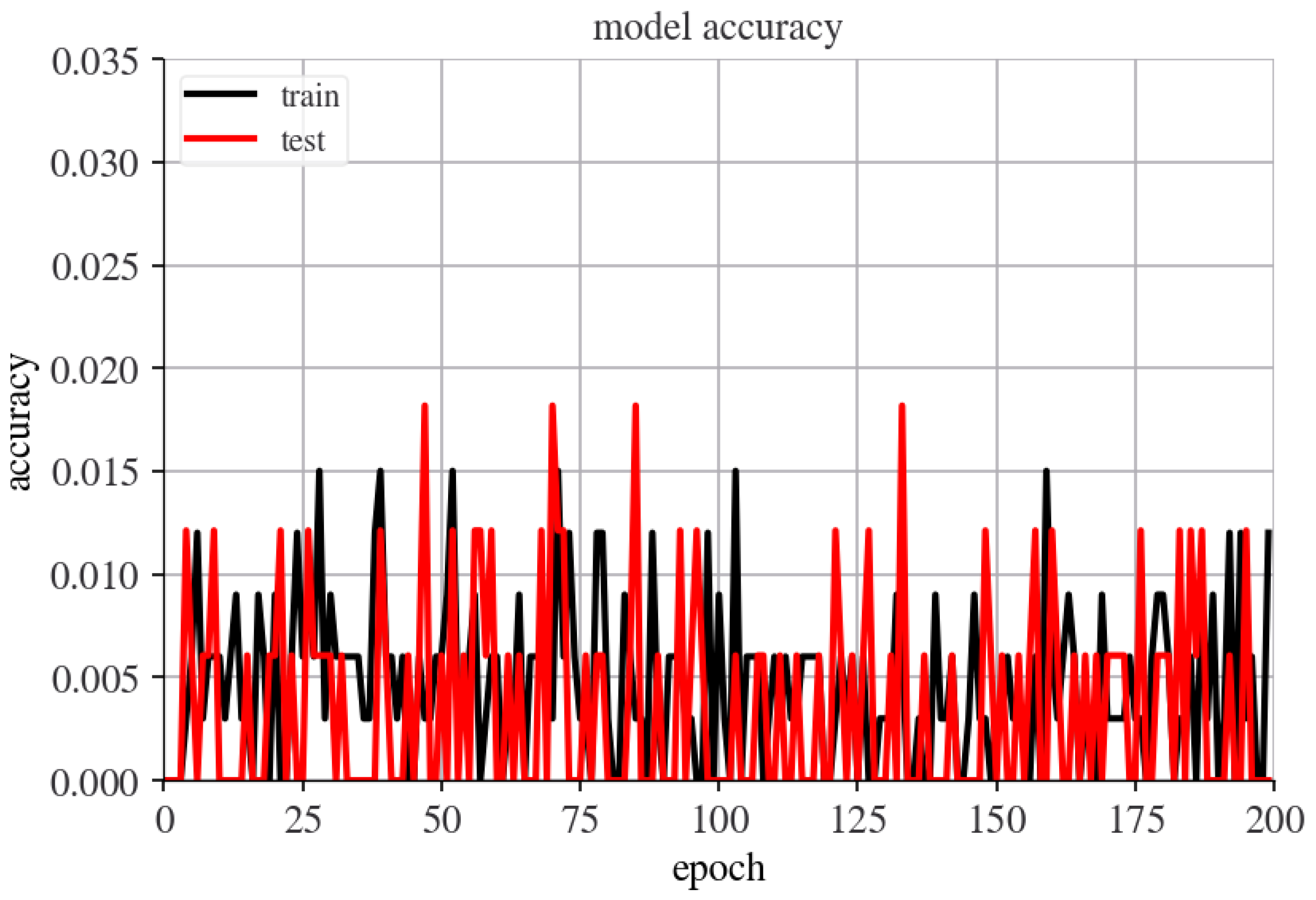
Figure 10 clearly shows that the KERAS model predicts very well the temperature reading of TC1 thermo-couple readings. Two plots are provided below: model accuracy and model loss. The history for the validation dataset is labelled as a test dataset for the model. The accuracy of the deep learning model is shown in Figure 11.
From the plot of accuracy shown in Figure 11, it can be seen that there is comparable behaviour on both datasets (train and test). Since the trend for accuracy on both datasets is similar, the training is satisfactory.
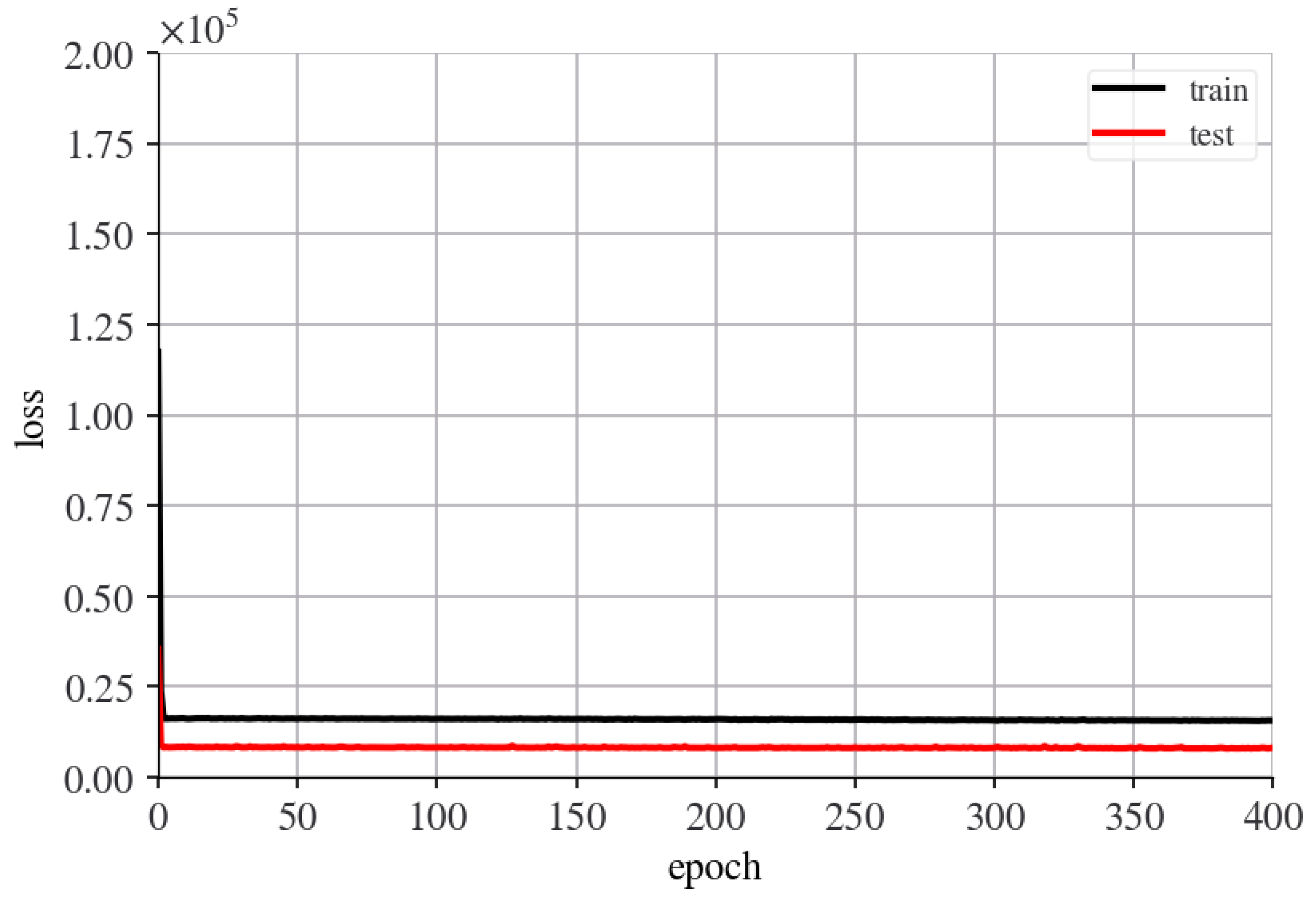
From the plot of loss shown in Figure 12, we can see that the model has comparable performance on both train and validation datasets (labelled as a test). If these parallel plots start to depart consistently, it might be a sign to stop training at an earlier epoch.
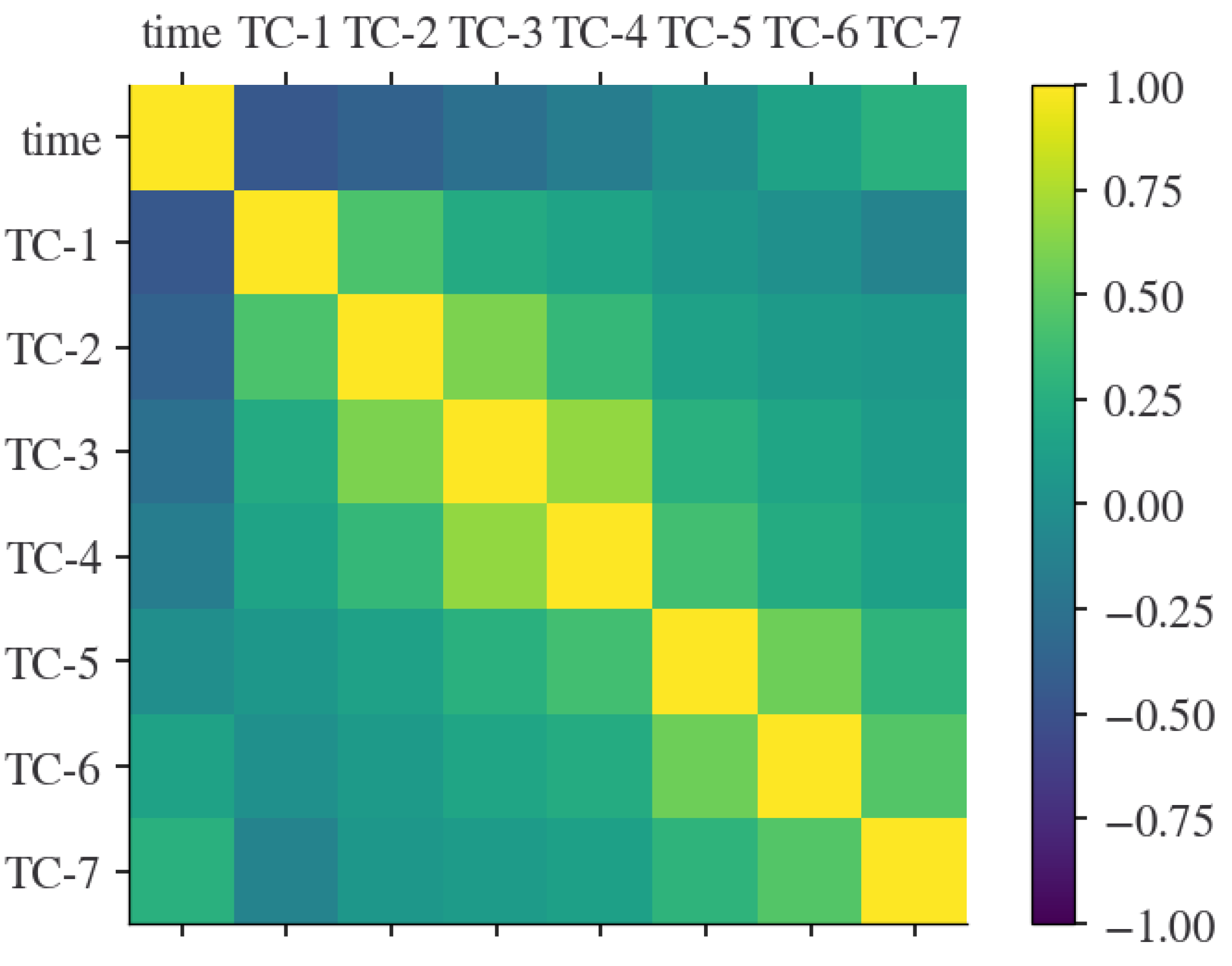
It is possible to calculate the correlation between each pair of attributes. This is called a correlation matrix. The correlation matrix provides an indication of which variables have a high correlation with each other. The correlation applied in this work provides an indication of how related the changes are between the time and seven thermocouple readings. If they are positively correlated, these variables change in the same direction. If they are negatively correlated, then they change in opposite directions together (one goes up, one goes down). The correlation matrix temperature plot is shown in Figure 13.
Figure 13 presents a good correlation between the two proximate thermo-couples readings. The correlation matrix soot concentration plot is shown in Figure 14.
From Figure 14 we can see that there is a good correlation between the two proximate soot concentration sensors readings.
3.3. Thermodynamics Analysis Results of the Organic Rankine Cycle (ORC)
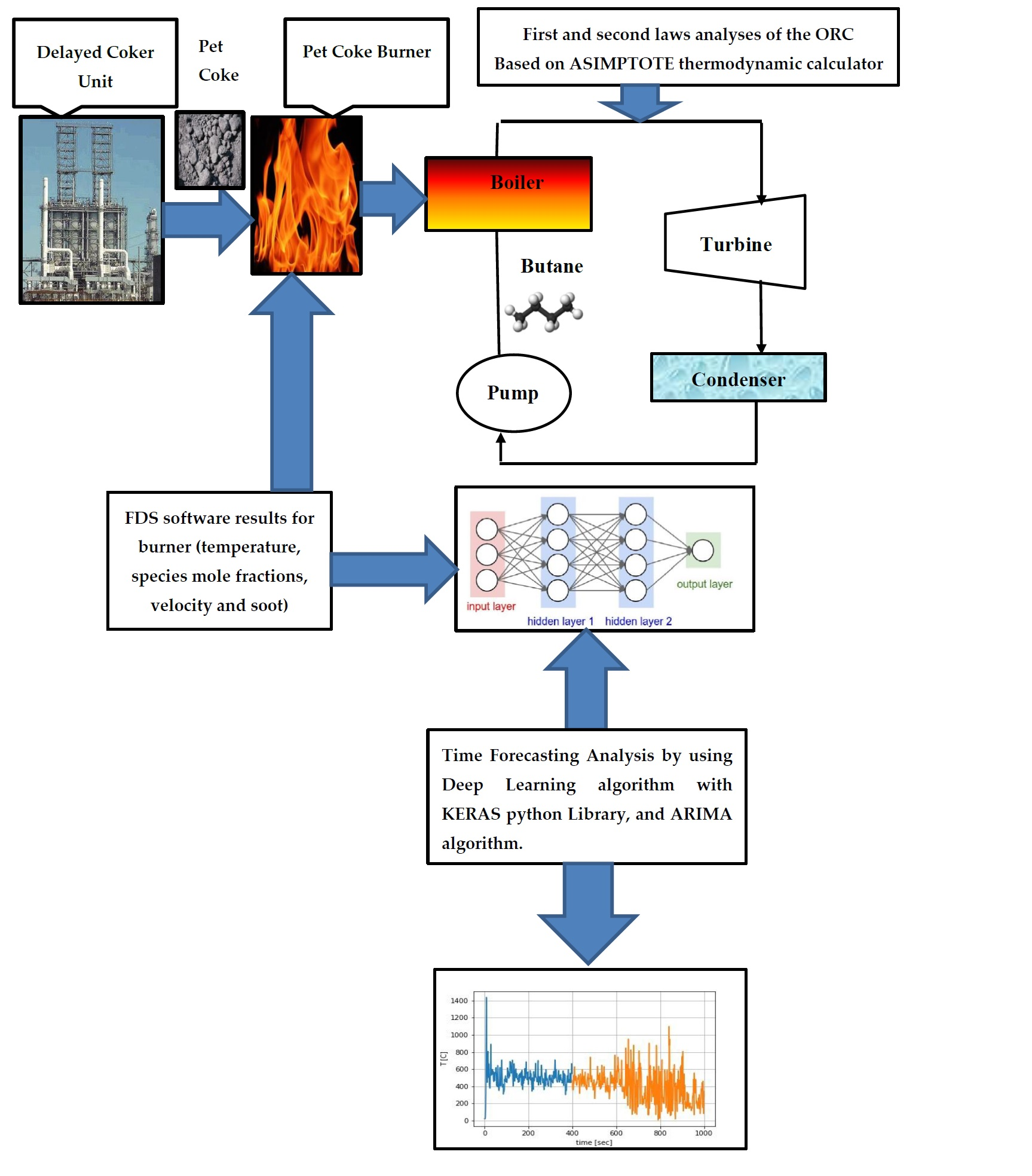
The thermodynamic analysis results are presented in this section. Table 1 includes the thermodynamic properties of the Butane obtained at different points of the ORC (see Figure 1).
Table 2 shows the heat rates of the boiler and the condenser, and the power produced by the turbine and invested in the pump. It is assumed that the mass flow rate of the Butane flows flowing inside the ORC system is 30.44 [kg/s] [26]. Butane is considered one of the best pure fluids in terms of exergy efficiency [26]. It has zero ozone depletion potential and low Global Warming Potential (about 4) [26]. It has low specific radiative forcing (RF) compared to Ethane and Propane [27]. It is considered flammable, highly stable and non-corrosive [28].
Table 2 clearly shows that the net power is equal to the net heat rate. Thus this thermodynamic cycle obeys the first law of thermodynamics. The calculated net power is similar to the net power reported in [26] which is also close to 3472 kW. The relative error is 4.8%. The thermal efficiency of the ORC is calculated by using the following equation:
Table 3 shows the entropies change rates of the main components of the Organic Rankine Cycle:
Table 3 clearly shows that the entropies change rates of each component inside the ORC are positive. Thus this thermodynamic cycle obeys the second law of thermodynamics.
4. Discussion
A thermodynamic analysis of Organic Rankine Cycle (ORC) was carried out in this work. The Petroleum Coke burner supplied the required heat flux for the Butane Boiler. Pet-coke (Petroleum Coke) is a heavy crude oil refining coproduct. It is identified as a black-colored and carbon-rich solid. Despite the few human health or environmental risks posed by the exploitation of pet-coke, it has many industrial applications. It is mostly applied as a boiling and combusting fuel in industrial, power generation, and cement plants. pet-coke is considered a promising substitute for steam coal in power plants because of its higher heating value, carbon content, and low ash, compared to bituminous coals. However, pet-coke gasification is a difficult process because of its high content of fixed carbon and low volatile matter.
This paper presents a thermodynamic analysis of Organic Rankine Cycle (ORC). The algorithm is composed of CFD modelling of hydrodynamics, heat transfer, and pet-coke combustion. Based on the CFD results, Time Forecasting Modelling Behavior of pet-coke combustion was applied by using Artificial Intelligence (AI) Algorithms. Fire Dynamics Simulator software (FDS) was applied in order to simulate pet-coke combustion. The FDS calculation results were validated by comparing the temperature of the gaseous mixture and CO2 mole fraction to the literature. The maximum flame temperature of the pet-coke is about: 1440 °C. It is similar to the temperature reported in the literature which is about 1400 °C. The maximal carbon dioxide mole fraction is 15.0%. It is similar to the carbon dioxide mole fraction reported in the literature which is 14.5%.
An Artificial Intelligence (AI) time forecasting analysis was performed on this work. The AI algorithm was applied to the temperature and carbon dioxide and monoxide sensors readings. Two Python libraries were applied in order to forecast the time behaviour of the thermocouple readings: Stats models—ARIMA (Auto Regressive Integrated Moving Average) and KERAS—Deep learning library. ARIMA is a class of models that captures a suite of different standard temporal structures in time series data. Keras is a Python library for deep learning that runs on top of Tensor-Flow. It was developed in order to perform deep learning models as fast and easy as possible for research and development. The calculated net power of the ORC cycle is similar to the net power reported in the literature. The proposed ORC obeys the first and second laws of thermodynamics.
5. Conclusions
The aim of this research is to investigate whether the pet-coke burner can provide the necessary heat flux for the Organic Rankine Cycle (ORC) operation. Butane has been employed as a working fluid in the ORC. Butane is considered one of the best pure fluids in terms of exergy efficiency. It has low specific radiative forcing (RF) compared to Ethane and Propane. It has zero ozone depletion potential and low Global Warming Potential (about 4).
This paper presents a CFD modeling of hydrodynamics and pet-coke combustion. Based on the CFD results, Time Forecasting Modelling Behavior of pet-coke combustion was applied by using Artificial Intelligence (AI) Algorithms. The simulation of pet-coke combustion was carried out by using Fire Dynamics Simulator software (FDS). Thermodynamic analysis was carried out on the ORC. It was observed that the pet-coke particles are mostly applied in Heat Recovery Steam Generator (HRSG), in Integrated Gasification Combine Cycle (IGCC), in Circulating Fluidized Bed (CFB) power plants, or in Rotary Kilns. To the best of my knowledge, it is probably the first time that a small-scale pet-coke box burner has been implemented as a heat source for operating Organic Rankine Cycle with butane working fluid. There are several applications pet-coke ORC Power systems. For example, the ORC power plant can be close to the refinery where the refinery uses its electric power. Green Hydrogen required for Hydrocracking and Hydrodesulfurization (HDS) reactions may be produced by water splitting. This system may be also applied for a backup solar power cycle. As far as I know, this work is the first coupled CFD simulation of pet-coke burner with ARIMA and deep learning algorithms and ASIMPTOTE online thermodynamic calculator. The numerical simulation results were carried out by using up-to-date computational software. The calculated temperatures and carbon dioxide mole fraction are similar to these values reported in the literature. Time series forecasting problems are a difficult type of predictive modeling problem. Unlike regression forecasting modeling, time series also adds the complexity of sequence dependence among the input variables. A powerful type of neural network designed to handle this time sequence dependence. The time forecasting capabilities of ARIMA and CNN methods are demonstrated in this work.
The convolutional neural network developed in this work contains eight hidden layers. RELU activation function was employed. This neural network was trained with several time-dependent CFD output files (including an additional FDS model which simulates Heptane burner). In all of them, the deep learning analysis proved that this CNN achieved excellent temperature predictions and provided a good theoretical verification of CNN for modelling pet-coke combustion. LSTM networks may be applied for time forecasting. The model accuracy and model loss plots show comparable performance (train and test datasets). The first thermodynamic equation was applied in order to evaluate the thermal power generated by the ORC turbine. It is assumed that the mass flow rate of the Butane flows flowing inside the ORC system is 30.44 [kg/s]. The thermal power generated by the turbine is 3.5 MW. The calculated net power is similar to the net power reported in the literature which is also close to 3472 kW. The relative error is 4.8%. The thermal efficiency of the ORC is 20.4%. It was demonstrated that the ORC system’s energetic system obeys the first and second laws of thermodynamics. The pet-coke burner can provide the necessary heat flux needed for the boiler operation. Thus this system is feasible. It is possible to produce green hydrogen from this reaction by using methane thermal decomposition. The hydrogen production system is composed of a pet-coke burner and a catalyst bed reactor. The heat produced from the pet-coke combustion can be utilized for maintaining the decomposition reaction of methane into hydrogen inside the catalyst bed. Another possibility is to utilize the electricity produced in the turbine for green hydrogen production by utilizing water-splitting technology.
Funding
This research has not received external funding.
Institutional Review Board Statement
Not applicable.
Informed Consent Statement
Not applicable.
Data Availability Statement
Not applicable.
Conflicts of Interest
The author declares no conflict of interest.
Abbreviation
| AI | Artificial Intelligence |
| ANN | Artificial Neural Network |
| ARIMA | Auto Regressive Integrated Moving Average |
| CFB | Circulating Fluidized Bed |
| CFD | Computational Fluid Dynamics |
| CNN | Convolutional Neural Networks |
| FCC | Fluid Catalytic Cracking |
| FDS | Fire Dynamics Simulation |
| FFNN | Feed Forward Neural Network |
| FVM | Finite Volume Method |
| HDS | Hydrodesulphurization |
| HSFO | High Sulfur Fuel Oil |
| HRR | Heat Release Rate |
| HRSG | Heat Recovery Steam Generation |
| IGCC | Integrated Gasification Combine Cycle |
| KERAS | Deep learning Python library |
| LES | Large Eddy Simulation |
| LSTM | Long Short Memory |
| ORC | Organic Rankine Cycle |
| SSSF | Steady State Steady Flow |
| Pet Coke | Petroleum Coke |
| RELU | Rectified Linear Unit |
| RTE | Radiation Transport Equation |
| TCNN | Transpose Convolutional Neural Networks |
| Nomenclature | |
| gravity acceleration in [m/s2] | |
| specific enthalpy of the stream in [kJ/kg] | |
| mass flow rate entering to the control volume in [kg/s] | |
| heat intecation rate invested/produced in the control volume in [kW] | |
| power in [kW] | |
| entropy change rate in [kW/K] | |
| specific entropy of the stream in [kJ/(kg K] | |
| temperature in [K] | |
| time in [K] | |
| velocity of the stream in [m/s] | |
| height of the stream in [m] | |
| Subscripts | |
| boiler | |
| condenser | |
| control volume | |
| leaving | |
| Heat Release Rate | |
| leaving | |
| net | |
| pump | |
| turbine | |
| Greek letters | |
| thermal efficency of the Organic Rankine Cycle | |
| density in [kg/m3] | |
References
- Eslami Afrooz, I.E.; Chuan Ching, D.L. A Modified Model for Kinetic Analysis of Petroleum Coke. Int. J. Chem. Eng. 2019, 2034983. [Google Scholar] [CrossRef]
- Gigilio, R. The Power Option; Digital Refining: Croydon, UK, 2019. Available online: https://www.digitalrefining.com/article/1002284/the-power-option#.XwnO7G0zbX4 (accessed on 15 July 2021).
- Ramesh, K. Estimating Delayed Coker Yields; Digital Refining: Croydon, UK, 2020. Available online: https://www.digitalrefining.com/article/1002409/estimating-delayed-coker-yields#.XxLFQm0zbX5 (accessed on 15 July 2021).
- Chang, J.; Wang, G.; Lan, X.; Gao, J.; Zhang, K. Computational Investigation of a Turbulent Fluidized-bed FCC Regenerator. Ind. Eng. Chem. Res. 2013, 52, 4000–4010. [Google Scholar] [CrossRef]
- Grace, J.R.; Taghipour, F. Verification and validation of CFD models and dynamic similarity for fluidized beds. Powder Technol. 2004, 139, 99–110. [Google Scholar] [CrossRef]
- Hamadeh, H.; Toor, S.Y.; Douglas, P.L.; Sarathy, S.M.; Dibble, R.W.; Croiset, E. Techno-Economic Analysis of Pressurized Oxy-Fuel Combustion of Petroleum Coke. Energies 2020, 13, 3463. [Google Scholar] [CrossRef]
- Shen, J.; Schmetz, E.; Stiegel, G.J.; Winslow, J.C.; Kornosky, R.M.; Madden, D.R.; Jain, S.C. Early Entrance Coproduction Plant—The Pathway to the Commercial CTL (Coal-to-Liquids) Fuels Production; Davis, B.H., Occelli, M.L., Eds.; Elsevier B.V.: Amsterdam, The Netherlands, 2007; Volume 163, pp. 315–325. ISBN 9780444522214. ISSN 0167-2991. [Google Scholar] [CrossRef]
- Lattimer, B.Y.; Hodges, J.L.; Lattimer, A.M. Using machine learning in physics-based simulation of fire. Fire Saf. J. 2020, 114, 102991. [Google Scholar] [CrossRef]
- Hodges, J.L. Predicting Large Domain Multi-Physics Fire Behavior Using Artificial Neural Networks. Ph.D. Thesis, Virginia Polytechnic Institute and State University, Blacksburg, VA, USA, 2018. [Google Scholar]
- Sun, Y.; Wang, J.; Zhu, W.; Yuan, S.; Hong, Y.; Mannan, M.S.; Wilhite, B. Development of Consequent Models for Three Categories of Fire through Artificial Neural Networks. Ind. Eng. Chem. Res. 2020, 59, 464–474. [Google Scholar] [CrossRef]
- McGrattan, K.B. Fire Dynamics Simulator (Version 5)—Technical Reference Guide Volume 1: Mathematical Model; NIST Special Publication 1018; National Institute of Standards and Technology U.S.: Washington, DC, USA, 2010. [Google Scholar]
- McGrattan, K.B.; Forney, G.P. Fire Dynamics Simulator (Version 5)—User’s Guide; NIST Special Publication 1019; National Institute of Standards and Technology U.S.: Washington, DC, USA, 2010. [Google Scholar]
- McGrattan, K.B. Numerical Simulation of the Caldecott Tunnel Fire, April 1982; NISTIR 7231; National Institute of Standards and Technology, U.S.: Washington, DC, USA, 2005. [Google Scholar]
- Davidy, A. CFD Simulation of Forced Recirculating Fired Heated Reboilers. Processes 2020, 8, 145. [Google Scholar] [CrossRef] [Green Version]
- Magee, J.S. Fluid Catalytic Cracking: Science and Technology, Studies. In Studies in Surface Science and Catalysis; Delmon, B., Yates, J.T., Eds.; Elsevier Science Publishers: Amsterdam, The Netherlands, 1993. [Google Scholar]
- Pedersen, M.N.; Nielsen, M.; Clausen, S.; Jensen, P.A.; Jensen, L.S.; Johansen, K.D. Imaging of Flames in Cement Kilns to Study the Influence of Different Fuel Types. Energy Fuels 2017, 31, 11424–11438. [Google Scholar] [CrossRef] [Green Version]
- Machine Learning Mastery. Available online: https://machinelearningmastery.com/backtest-machine-learning-models-time-series-forecasting/ (accessed on 15 July 2021).
- Brownlee, J. Deep Learning with Python, Develop Deep Learning Models on Theano and Tensor Flow using KERAS; Version 1.18; Machine Learning Mastery: Vermont Victoria, Australia, 2019. [Google Scholar]
- Brownlee, J. Deep Learning for Time Series Forecasting Predict the Future with MLPs, CNNs and LSTMs in Python; Version 1.6; Machine Learning Mastery: Vermont Victoria, Ausralia, 2019. [Google Scholar]
- Brownlee, J. Machine Learning Mastery with Python: Understand Your Data, Create Accurate Models and Work Projects End-to-End; Version 1.18; Machine Learning Mastery: Vermont Victoria, Ausralia, 2020. [Google Scholar]
- Van Wylen, G.J.; Sonntag, R.E. Fundamentals of Classical Thermodynamics, 3rd ed.; SI Version; John Wiley and Sons Inc: Toronto, ON, Canada, 1985. [Google Scholar]
- ASIMPTOTE. Available online: http://www.asimptote.nl/software/fluidprop/fluidprop-calculator (accessed on 8 October 2020).
- Ahmed, D.F.; Ateya, S.K. Modelling and Simulation of Fluid Catalytic Cracking Unit. J. Chem. Eng. Process Technol. 2016, 7, 308. [Google Scholar] [CrossRef] [Green Version]
- Commandre, J.L.; Salvador, S. Lack of correlation between the properties of a petroleum coke and its behavior during combustion. Fuel Process. Technol. 2005, 86, 795–808. [Google Scholar] [CrossRef] [Green Version]
- Sandmo, T. The Norwegian Emission Inventory 2009: Documentation of Methodologies for Estimating Emissions of Greenhouse Gases and Long-Range Transboundary Air Pollutants; Statistics Norway/Department of Economics, Energy and the Environment Statistics: Oslo, Norway, 2009. [Google Scholar]
- Castelli, A.F.; Elsido, C.; Scaccabarozzi, R.; Nord Lars, O.; Martelli, E. Optimization of Organic Rankine Cycles for Waste Heat Recovery from Aluminum Production Plants. Front. Energy Res. 2019, 7, 44. [Google Scholar] [CrossRef] [Green Version]
- Hodnebrog, Ø.; Dalsøren, S.B.; Myhre, G. Lifetimes, direct and indirect radiative forcing, and global warming potentials of ethane (C2H6), propane (C3H8), and butane (C4H10). Atmos. Sci. Lett. 2018, 19, e804. [Google Scholar] [CrossRef]
- Bronicki, L.Y. History of Organic Rankine Cycle systems, in Organic Rankine Cycle (ORC) Power Systems Technologies and Applications. In Woodhead Publishing Series in Energy; Macchi, E., Astolfi, M., Eds.; Elsevier: Amsterdam, The Netherlands, 2017. [Google Scholar]
Figure 1.
Schematics of an organic rankine cycle system based on pet coke burner.

Figure 2.
Geometrical model of the pet-coke burner.

Figure 3.
Schematics of the computational process algorithm of the pet-coke burner.

Figure 4.
Temperature field (°C) of the flue gaseous mixture inside the burner at t = 60.7 s.

Figure 5.
Velocity field (m/s) of the flue gaseous mixture at t = 60.7 s.

Figure 6.
Heat Release Rate (HRR) of the pet-coke particles.

Figure 7.
Temperature readings of the three thermocouples TC1, TC4 and TC7.

Figure 8.
Carbon dioxide readings of three sensors inside the burner.

Figure 9.
Comparison between computational temperature reading and time forecasting with the ARIMA model.
Figure 9.
Comparison between computational temperature reading and time forecasting with the ARIMA model.

Figure 10.
Prediction of the temperature reading using a simple multilayer perceptron model with a time lag, blue represents the whole dataset, green represents training and orange represents predictions.
Figure 10.
Prediction of the temperature reading using a simple multilayer perceptron model with a time lag, blue represents the whole dataset, green represents training and orange represents predictions.

Figure 11.
Plot of model accuracy on train and validation datasets.

Figure 12.
Plot of model loss on training and validation datasets.

Figure 13.
Correlation matrix temperature plot.

Figure 14.
Correlation matrix soot concentration plot.


Table 1.
Thermodynamic properties of Butane at different locations of the Organic Rankine Cycle (the locations are shown in Figure 1).
Table 1.
Thermodynamic properties of Butane at different locations of the Organic Rankine Cycle (the locations are shown in Figure 1).
| Point | Pressure [kPa] | Temperature [°C] | Enthalpy, h [kJ/kg] | Entropy, s [kJ/(kg K)] |
|---|---|---|---|---|
| 1 | 3905 | 164.2 | 770.5 | 2.3404 |
| 2 | 238 | 58.7 | 655.1 | 2.3550 |
| 3 | 238 | 24.5 | 232.7 | 0.9476 |
| 4 | 3905 | 25.9 | 239.6 | 0.9477 |
Table 2.
Heat and Power invested and produced in the Organic Rankine Cycle.
| Heat/Power | Value [kW] |
|---|---|
| 16,161 | |
| −12,856 | |
| 3305 | |
| 3513 | |
| −207.4 | |
| 3305 |
Table 3.
Entropies change rates of the main components of the Organic Rankine Cycle.
| Component | Value [kW/K] |
|---|---|
| 0.444 | |
| 0.277 | |
| 0.003 | |
| 5.442 |
Publisher’s Note: MDPI stays neutral with regard to jurisdictional claims in published maps and institutional affiliations. |
© 2021 by the author. Licensee MDPI, Basel, Switzerland. This article is an open access article distributed under the terms and conditions of the Creative Commons Attribution (CC BY) license (https://creativecommons.org/licenses/by/4.0/).
Share and Cite
MDPI and ACS Style
Davidy, A. Thermodynamic Design of Organic Rankine Cycle (ORC) Based on Petroleum Coke Combustion. ChemEngineering 2021, 5, 37. https://0-doi-org.brum.beds.ac.uk/10.3390/chemengineering5030037
AMA Style
Davidy A. Thermodynamic Design of Organic Rankine Cycle (ORC) Based on Petroleum Coke Combustion. ChemEngineering. 2021; 5(3):37. https://0-doi-org.brum.beds.ac.uk/10.3390/chemengineering5030037
Chicago/Turabian StyleDavidy, Alon. 2021. "Thermodynamic Design of Organic Rankine Cycle (ORC) Based on Petroleum Coke Combustion" ChemEngineering 5, no. 3: 37. https://0-doi-org.brum.beds.ac.uk/10.3390/chemengineering5030037