Article

Intraparticle Model for Non-Uniform Active Phase Distribution Catalysts in a Batch Reactor

1
Chemical Sciences Department, University of Naples Federico II, IT-80126 Napoli, Italy
2
Laboratory of Industrial Chemistry and Reaction Engineering, FI-20500 Åbo Akademi, Finland
*
Author to whom correspondence should be addressed.
Submission received: 23 June 2021 / Revised: 8 July 2021 / Accepted: 12 July 2021 / Published: 19 July 2021
(This article belongs to the Special Issue Feature Papers in Chemical Engineering)

Abstract

:
The study and the understanding of the importance of the morphological properties of heterogeneous catalysts can pave the way for important improvements in the performance of catalytic systems. Non-uniform active phase distribution catalysts are normally adopted for consecutive reactions to improve the selectivity to the desired intermediate product. Attributes on which minor attention is paid, such as the distribution and thickness of the active phase, can be decisive in the final rationale of the catalyst synthesis strategy. Starting from a previous work, where a single non-uniform active phase model for catalyst particles was developed, a key step to control the entire system is to include the bulk-phase equations and related transport phenomena. For this purpose, this work proposes a modeling approach of a biphasic reactive system in a batch reactor in the presence of three different kinds of catalytic particles (egg shell, egg white, and egg yolk) whose distinction lies in the localization of the active zone. The reactive network consists of a couple of reactions in series, which take place exclusively on the solid surface, and the intermediate component is the main product of interest. To reveal the influence related to the type of catalyst, an extensive parametric study was conducted, varying several structural coefficients to highlight the changes in the intraparticle and bulk concentration profiles of the different chemical species. The main results can be considered of wide interest for the chemical reaction engineering community, as it was demonstrated that mass and heat transfer limitations affect the catalyst performance. For the chosen system, the egg shell catalyst normally led to better catalytic performances.

1. Introduction

The optimization of the performances of the heterogeneous catalysts is a key point in the design and optimization of a chemical reactor, thus the entire chemical plant. When faced with a complex reaction network, several aspects must be considered to optimize the yields of desired chemical components. For many of the heterogeneously catalyzed chemical systems, the intermediate is the desired component, thus a lowering in the product yield surely leads to less optimized processes. Moreover, often the side reactions can undergo a runaway, as for partial oxidation of olefines [1,2,3,4].
Typically, the catalytically active phase is dispersed on a support, which leads to an increase of the specific contact area. It was demonstrated that by confining the active phase in specific portions of the support can lead to high benefits in optimizing the yield of an intermediate, gaining better results compared to the ones obtainable with a uniform active phase distribution, which classically could lead to higher mass transfer limitation, such that the inner part of the catalyst could be hardly reached by the reactants by diffusion, thus a worse catalyst optimization [5,6].
The optimal design of the active phase distribution is an attractive opportunity to be considered, as it could lead to lower costs of the catalytic material overall, if the active phase is a high-prize metal.
It is possible to choose between different alternatives:
(1)
Uniform: the active phase if homogeneously distributed on the support.
(2)
Egg-shell: the active phase is located in the outer surface of the support.
(3)
Egg-white: the active phase is included in a region between the outer-shell and the inner-core.
(4)
Egg-yolk: the active phase is present in the inner-core of the support.
The correct design of the right active phase distribution within the support is still a real challenge [7] and a topic that requires high experimental and numerical efforts [8]. Modeling can surely help in the heterogeneous catalyst design as, knowing a-priori the intrinsic kinetics of a chemical reaction network, it can be possible to choose the best non-uniform active phase distribution option and optimize it, answering the following questions: How much active phase is really needed? Where should it be located?
Several models were reported in the literature, based on simplified approaches, either neglecting the dynamic term [9] or oversimplifying the fluid–solid and intraparticle phases [6], leading in every case to a rough estimation of the concentration and temperature profiles. Insights on the NUD experimental and modelling cases is reported in our previous publication [5].
The latest approach, published by us recently [5], allowed to develop a rigorous Non-Uniform active phase Distribution model (NUD) for a single particle. The results allowed to demonstrate that dependently on the kinetics of a chemical reaction, it is possible to design different NUD of a catalyst allowing the optimization of the yield of a desired chemical intermediate. Despite the promising application, efforts must be made to frame the developed model in a real case, thus a chemical reactor, coupling the mass and heat balance equation of the catalytic phase with the fluid bulk phase. In this way, the model can be considered a realistic tool to design an NUD heterogeneous catalyst for a selected chemical reaction, allowing both the description of experimental data and the simulation of optimal NUD catalysts.
For this reason, in the present work, NUD was coupled with the balance equations of a batch system, focusing the attention on consecutive reaction scheme (A→B→C), where the intermediate chemical specie B is the main product of interest. The model consists in a set of mass and energy balance equations, including the dynamic term, considering a spherical catalyst. A sensitivity study allowed to identify optimal conditions to maximize the yield of B. The reference particle is egg-shell type; comparisons with other active phase distributions were conducted.

2. Mathematical Model

The present model has been developed to describe a biphasic reactive system consisting of a liquid phase, containing the reagent, placed in contact with a defined quantity of heterogeneous catalyst in a batch reactor. The reactive network consists of two exothermic consecutive reactions, occurring exclusively in the active phase of the solid, therefore, to evaluate the variation of composition and temperature over time, for both phases, appropriate mass and energy balances were implemented. The singularity of this model consists of the different types of catalyst used, which have an active phase distribution that is found exclusively in the outer part (Egg Shell), in the central part (Egg White) or in the core (Egg Yolk) of the particle. Specific distribution functions of the catalytic phase were then developed to observe the response of the system under examination.

2.1. Reaction Rate Expressions

The reactive system under consideration consists of a couple of irreversible reactions in series. Reagent A is initially present in the liquid phase and then diffuses in the solid to reach the catalytically active zone. The stoichiometry is given below,
A r 1 B r 2 C ,   Δ r H j < 0
Assuming that both reactions are described by first-order kinetics, the reaction rate expressions used can be written as shown by Equations (1) and (2).
r 1 ( t , x ) = k 1 c A , s ( t , x )
r 2 ( t , x ) = k 2 c B , s ( t , x )
The reaction stoichiometry is synthesized in the matrix (3).
ν i j = [ 1 + 1 + 1 0 1 0 ]
The temperature dependence of the kinetic constants was evaluated with the modified Arrhenius law, using a reference temperature of Tref = 323.15 K (4).
k j ( t , x ) = k r e f j exp [ ( E A j R g ) ( 1 T s ( t , x ) 1 T r e f ) ]

2.2. Mass and Energy Balances

Under dynamic conditions, two mass balance equations, for the liquid and solid phases have been developed (5) and (6) [5,10]:
ε c i , l ( t ) t = k m a s p ( c i , l ( t ) c i , s ( t , x ) | x = 1 )
ε P c i , s ( t , x ) t = D e f f , i R p 2 ( 2 c i , s ( t , x ) x 2 + s x c i , s ( t , x ) x ) + Ω k ρ P j = 1 N ν i j r j ( t , x )
where km, in the liquid phase balance, represents the liquid–solid mass transfer coefficient, asp is the specific surface area, calculated according to Equation (7), and ε represents the volumetric ratio between the phases, obtained from the ratio between the particle density (ρP) and the catalyst bulk density (ρBulk) as shown in Equation (8).
a s p = 3 R P
ε = ρ P ρ B u l k
In the solid side, balance εP is the catalyst porosity, Deff,i is the effective molecular diffusivity, while s is the shape factor calculated assuming that the catalyst particles have a spherical shape.
As it is possible to note, the presence of the distribution function in the generation term makes it possible to discriminate the catalytically inert zone, in which only diffusive phenomena are observed (Ωk = 0), from the active one (Ωk = 1), where it the chemical reaction is also present.
To solve the system of partial differential equations, boundary conditions were formulated. The following system of differential Equation (9) reproduces the behavior of the reactive system at the center of the catalytic particle (x = 0) and at the liquid–solid interface on its external surface (x = 1),
{ c i , s ( t ) x | x = 0 = 0 D e f f , i R P c i , s ( t ) x | x = 1 = k m ( c i , l ( t ) c i , s ( t ) | x = 1 )
Energy balance for both liquid and solid phases were implemented in Equations (10) and (11):
( i = 1 N c p , i c i , l ( t ) ) T l ( t ) t = h a s p ( T l ( t ) T s ( t , x ) | x = 1 ) ε U A ( T l ( t ) T j )
( c p , P ( 1 ε P ) + i = 1 N c p , i c i , l ( t ) ε P ) T s ( t , x ) t = k T , P R p 2 ( 2 T s ( t , x ) x 2 + s x T s ( t , x ) x ) Ω k ρ P j = 1 N Δ r H j r j ( t , x )
where cp,i and cp,P, represent the specific heat of the fluid component and of the catalytic particle, respectively, while kT,P is the particle heat conductivity.
The parameter h is the thermal resistance at the liquid–solid interface, calculated with the Chilton–Colburn analogy, which provides the ratio between the fluid heat conductivity (kT,l) and the mass transfer coefficients (12) [11].
h = k m D e f f ( ρ l D e f f c p , l k T , l ) 1 3 k T , l
As revealed, in the liquid side balance, there is also an energy exchange term with the external environment useful for simulating the dissipation of a part of the energy resulting from the reaction. UA represents the external thermal resistance, while Tj is the external temperature.
The boundary conditions useful for the description of the energy balance are reported in expression (13).
{ T s ( t ) x | x = 0 = 0 T s ( t ) x | x = 1 = h ( T l ( t ) T s ( t ) | x = 1 )
Finally, the catalytic efficiency was obtained through Equation (14) [12].
η ( t ) = 0 1 ( r 1 ( t , x ) R P x s 1 ) d x r 1 ( t , x ) | x = 1 0 1 ( R P x s 1 ) d x

2.3. Distribution Function

To simulate the non-uniform active phase in the catalyst, it was necessary to formulate distribution functions, which depend on the radial coordinate (x) of the spherical particle, obtained from the ratio x = r/RP. Step functions (Ωk) were used including the following parameters: smoothing factor b, useful for evaluating the slope of the curve and inflection points as and ast, for the definition of the distribution ranges. The functions used are reported in Equations (15)–(17) [13].
Egg Shell (ES)
Ω 1 ( x ) = 0.5 + 0.5 tanh ( x a 1 b )
Egg Yolk (EY)
Ω 2 ( x ) = 0.5 0.5 tanh ( x a 2 b )
Egg white (EW)
Ω 3 ( x ) = 0.5 tanh ( x a 3 1 b ) 0.5 tanh ( x a 32 b )
For egg shell distribution, the thickness of the active phase is 1 − a1, while it is equal to a2 for the egg yolk catalyst. Regarding the distribution of egg white, two coordinates are needed for the catalyst; therefore, the thickness of the active phase can be defined by a31-a32. The dimensions of the catalytic thickness are the same in all distributions.

2.4. Numerical Methods

The mathematical model was developed in gPROMS ModelBuilder v 4.0.0 [14], solving the system of partial differential equations, setting 100 grid points for the dimensionless radial coordinate of the particles. The numerical method used was the DASOLV, which it is based on backward differentiation formulas with variable time step/variable order.

3. Results and Discussion

3.1. Model Validation: Standard Simulation

In this work, several simulations of the intraparticle model with non-uniform active phase distribution in a batch reactor were conducted. The same simulations were developed using three different categories of spherical catalysts, which are distinguished from each other by the distribution of the active phase, in order to observe a high production of the main product, the reaction intermediate B.
Starting from a standard simulation, obtained by selecting a set of parameters that could well describe the reactive process, the subsequent simulations were performed by decreasing and increasing (lower and higher value, respectively) every single coefficient significantly influencing the reaction environment. Parameters were set taking inspiration, as in our previous work [5], by the physico-chemical properties of the components involved in the catalytic reaction of synthesis of ethylene oxide [5,6]. The coefficients used for the standard simulation are shown in Table 1.
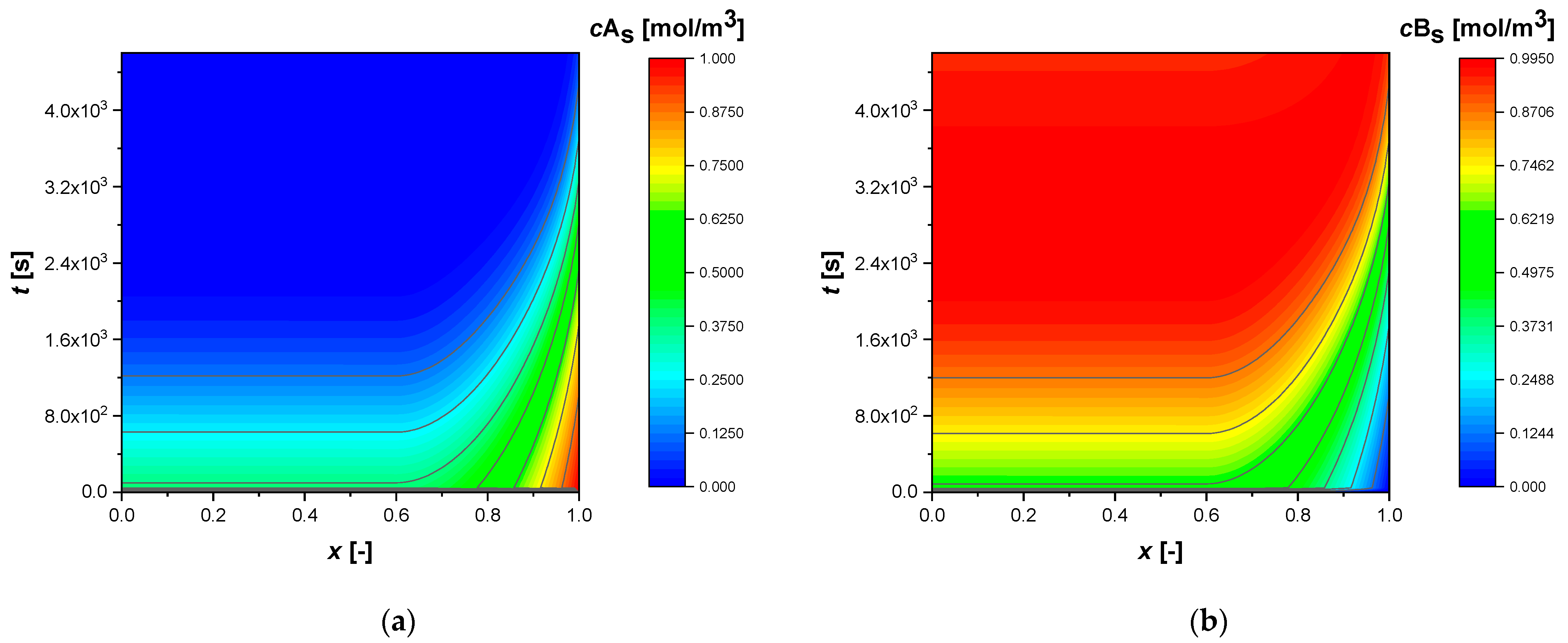
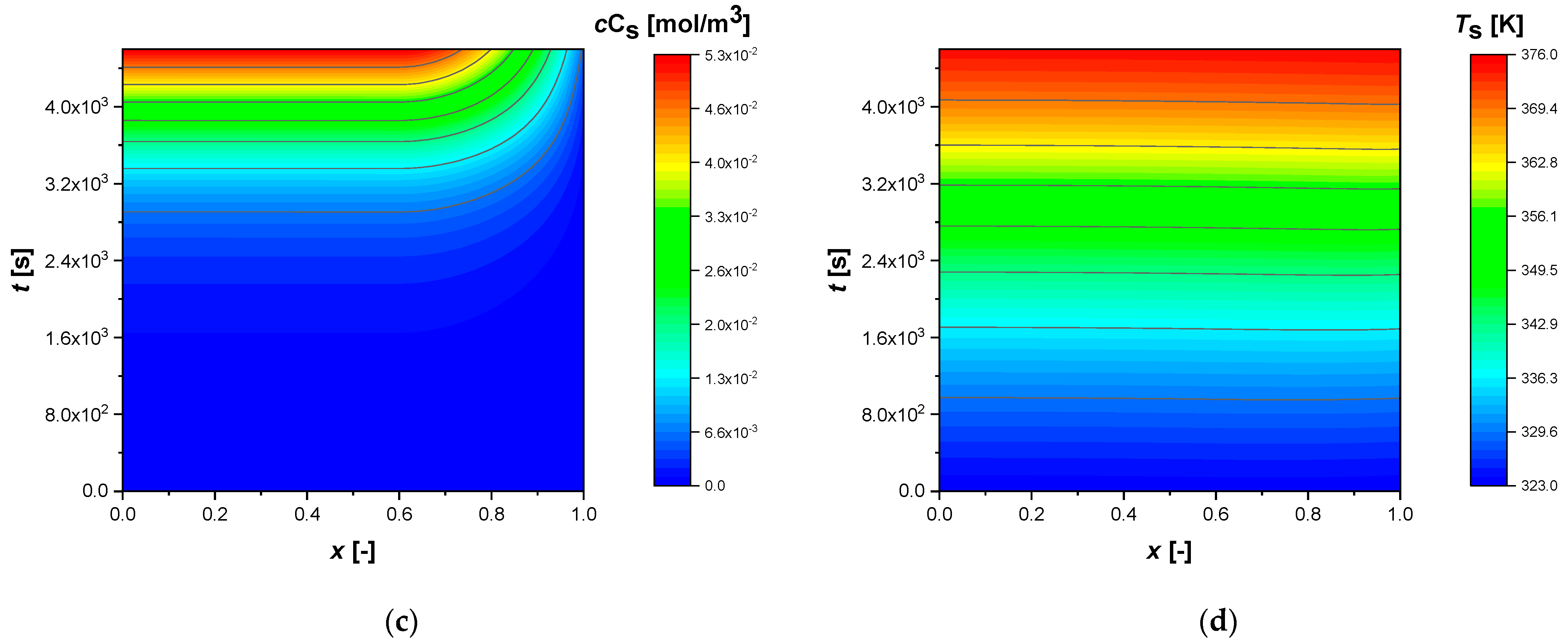
All simulations were conducted until a conversion of approximately 92% of reactant A was achieved. The intraparticle concentrations and temperature profiles, from the standard simulation, calculated for egg shell, egg white, and egg yolk, respectively, are shown in the contour plots, Figure 1, Figure 2 and Figure 3.
As revealed, egg shell catalysts (Figure 1) lead to flat profiles in the inner core of the catalyst, where the reaction does not occur due to the absence of the active phase, while strong concentration gradients are expected in the outer shell where the chemical reaction is promoted by the active phase. Egg white NUD modelling, allow to predict high gradients only where the active phase is present (Figure 2). The reaction time increases dramatically when the catalytic phase is located in the innermost parts of the particle (egg yolk case, Figure 3), due to the internal diffusive phenomena (non-flat intraparticle profiles). The external mass transfer coefficient (km), on the other hand, is sufficiently high to make the resistance to diffusion in the stagnant fluid film negligible. The same evaluation can be made with respect to the coefficient of thermal resistance at the liquid–solid interface (h), which has a value high enough to make its effects negligible. Moreover, it is important to consider that under standard conditions, the system was considered adiabatic (UA = 0), thus the worse possible situation. In real cases, heat exchange is normally provided, leading to a consequent smoothing of the temperature increase.
In all the simulations, reagent A is consumed in the active region of the catalyst (Figure 1, Figure 2 and Figure 3), spreading and accumulating more in cases where the active phase is located deep in the particle (Figure 3). Intermediate B is produced and consumed in the same regions, reaching a maximum more or less rapidly, depending on the NUD.
Similarly to B, the component C produced and diffused in the particle, accumulates more in the egg yolk (Figure 3) case due to the diffusive phenomena that slow down its release in the bulk.
In all cases, the profiles show an increase in temperature throughout the particle of approximately 53 K.
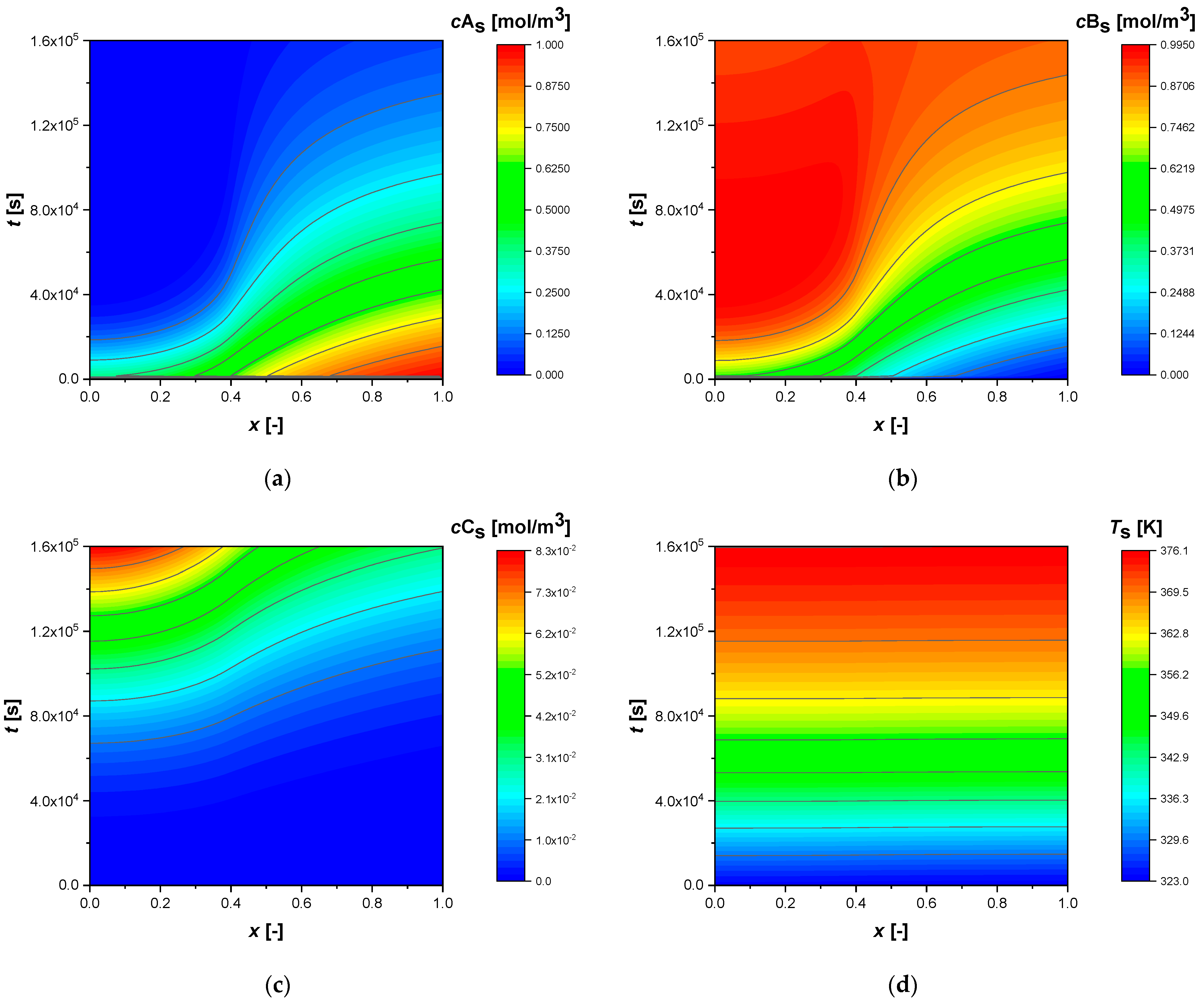
The reactant conversion, the product selectivity and efficiency of the chemical reaction in the liquid phase were calculated for each case studied. Their profiles and temperature over time are shown in Figure 4, for the egg shell, egg white, and egg yolk cases.
As revealed by the figures, a high selectivity of the intermediate product is observed, which tends to decrease in EW and EY cases (Figure 4a). Its accumulation in the catalytic zone, caused by the diffusion resistance towards the outside, increases the rate of the second reaction and, consequently, the quantity of C produced.
The yield of the desired product faithfully follows the conversion profile, deviating slightly at high times in the two final simulations. Finally, an increase in the temperature of the liquid phase of about 50 K in all cases was observed (Figure 4b).
The catalytic efficiency of the egg shell decreases drastically after the initial maximum, while in the other two cases, it settles down to, 0.41 and 0.61 for egg white and egg yolk, respectively (Figure 4c).

3.2. Parametric Investigation

In order to study the response of the model to parametric variation, several simulations were conducted. For each parameter considered, a lower and a higher value was chosen starting from the standard value. The results were reported as comparison graphs of the bulk concentrations and intraparticle profiles of the components at the steady state. The coefficients used in the parametric study are shown in Table 2 by decreasing or increasing the values of the parameters with respect to the standard.

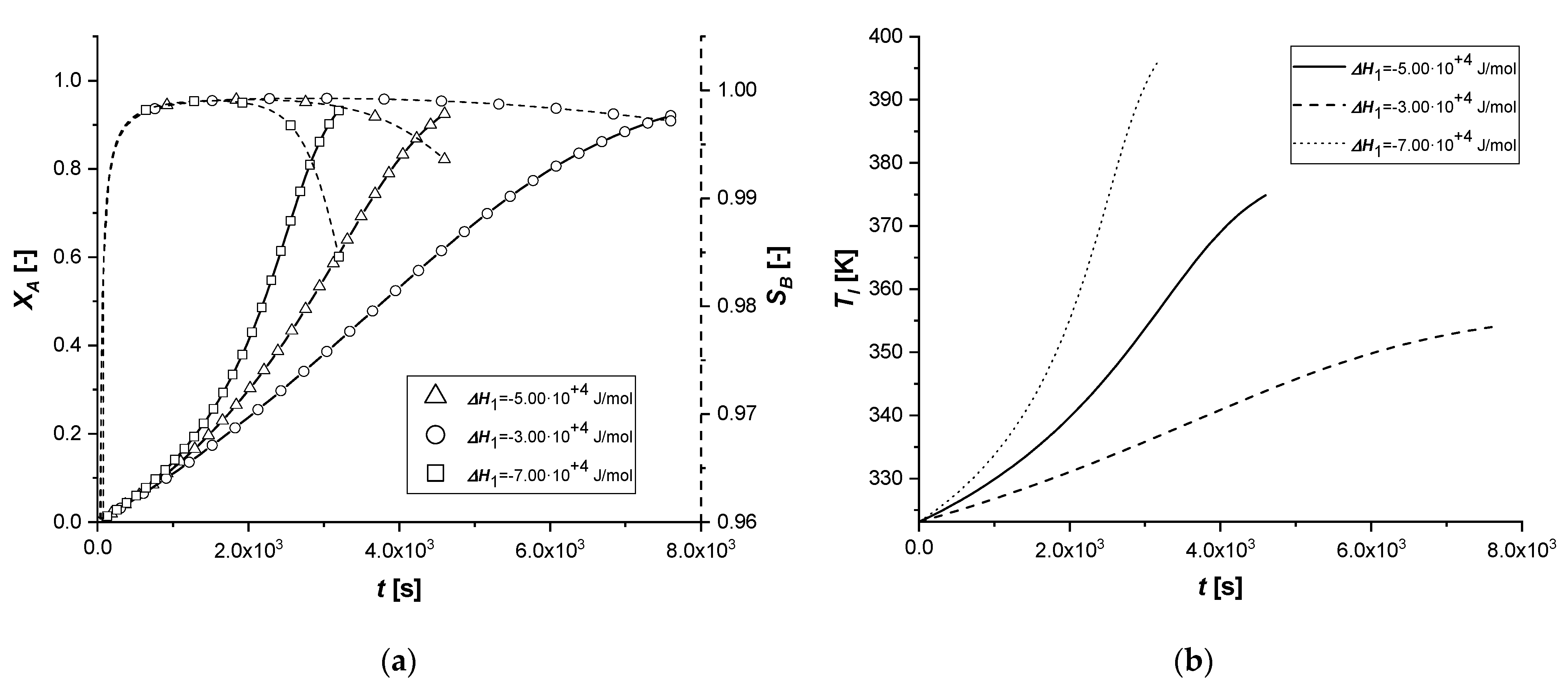
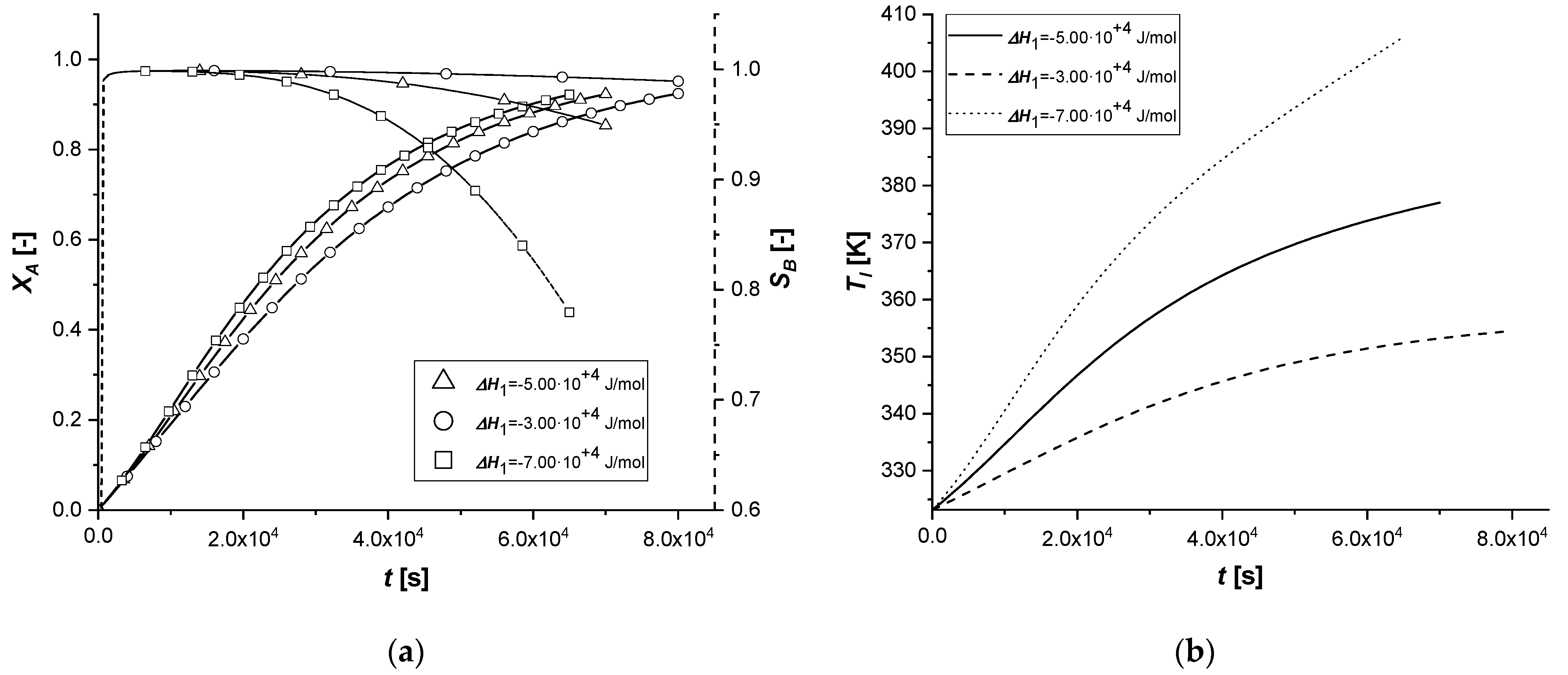
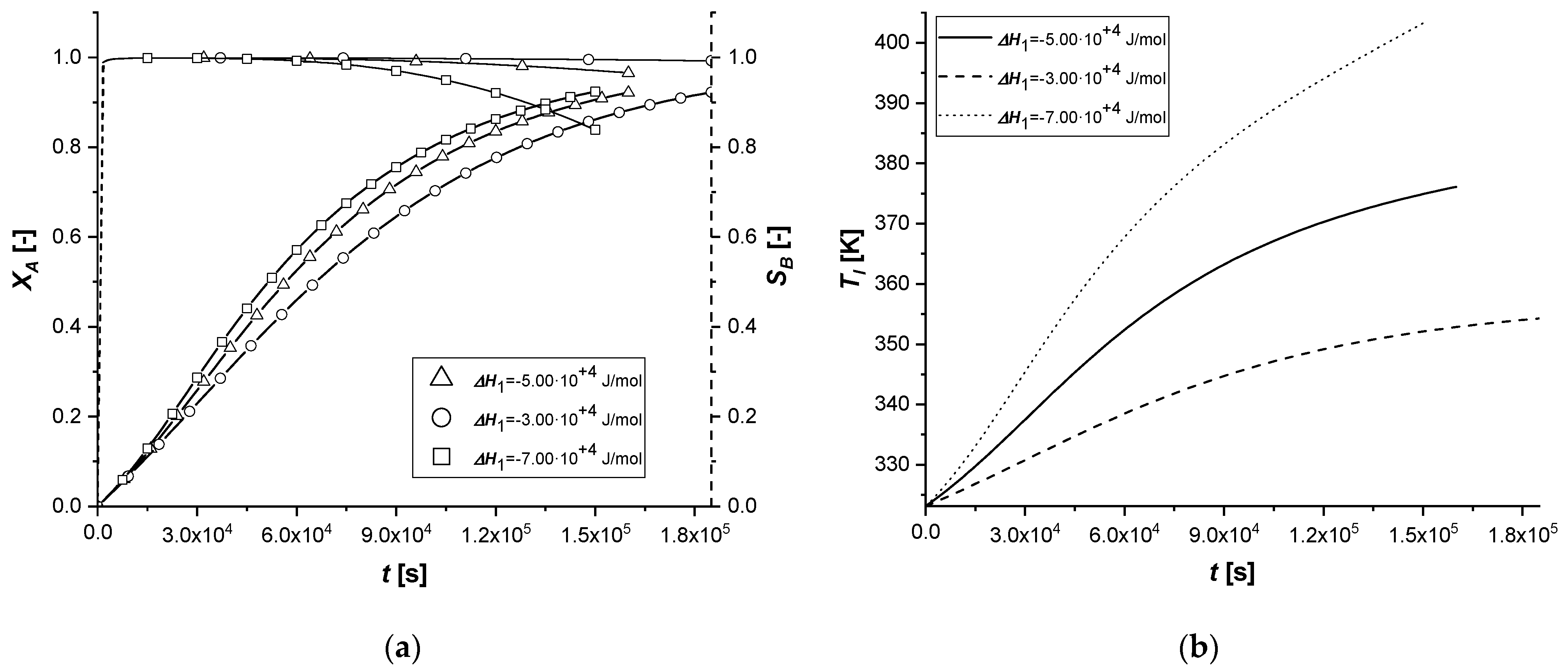
3.2.1. Reaction Enthalpy

The consequent variation of the enthalpy of the first reaction determines the lowering or increase of the quantity of energy released by the reaction itself. As a result, the overall system temperature will be lower or higher than the standard simulation. The parameter affects indirectly the reaction rate and particularly on the kinetic constant calculated with the modified Arrhenius equation which is a function of the operation temperature.
The comparison between the solid side and liquid side concentration profiles computed for all the catalytic cases are reported in Supplementary Materials in Figures S1–S9. The details of each conversion, selectivity, and liquid side temperature profiles are displayed in Figure 5, Figure 6 and Figure 7.
It can be noted that, in all cases, as the thermodynamic parameter increases, both reactive processes are enhanced; moreover, it is interesting to note that the first catalytic system behaves differently from the other ones.
In fact, if in the ES case the consumed quantity of A seems to be very sensitive for the variation of the coefficient, the same behavior is not observed in the case of EW and EY. Its consumption is clearly limited by internal diffusion resistance. As the component slowly reaches the active phase of the catalyst, promoting the formation of the intermediate, the increase in the reaction rate, due to temperature, causes an accelerated consumption of B available close to the catalytic site. In these two cases, the quantity of C obtained is therefore higher.
Ultimately, it can be assumed that the use of ES type catalysts is favorable if it is desired to improve the production of the intermediate in exothermic reactions if severe limitations of internal diffusion arise.
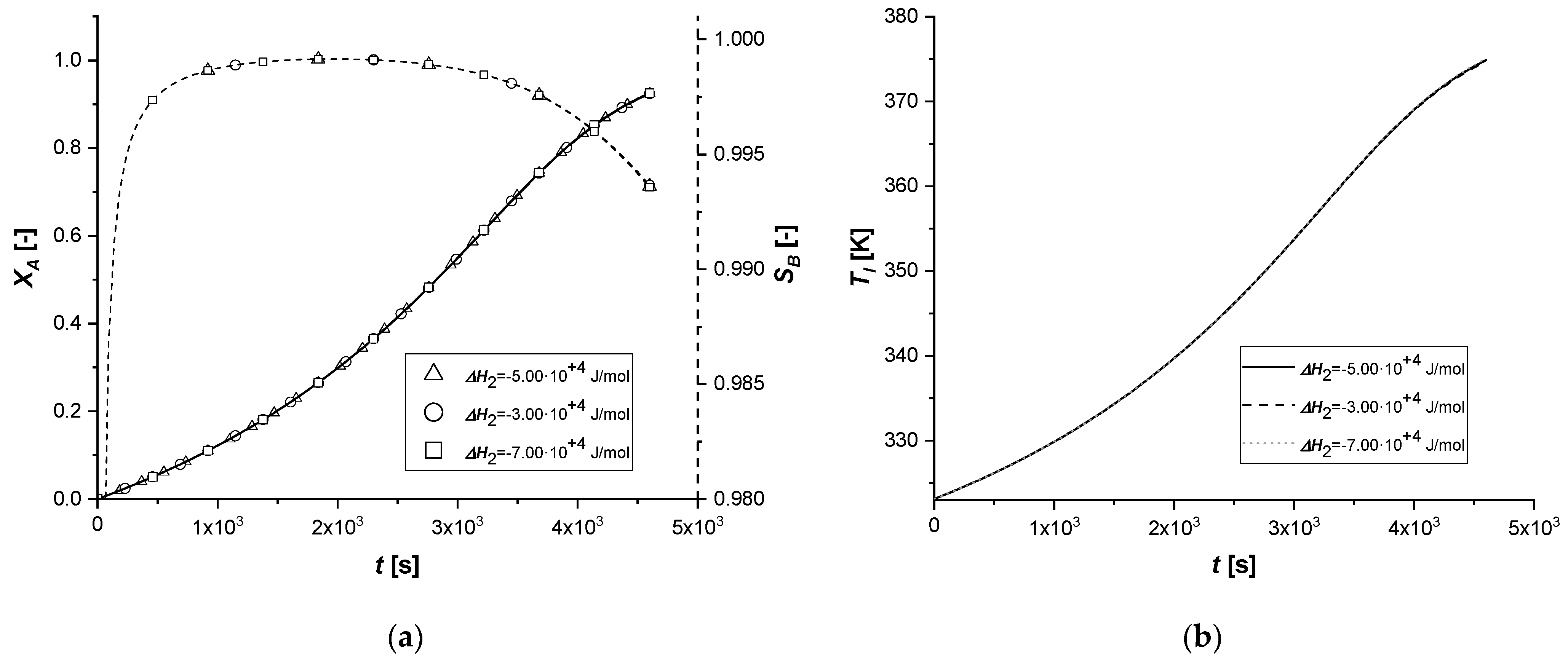
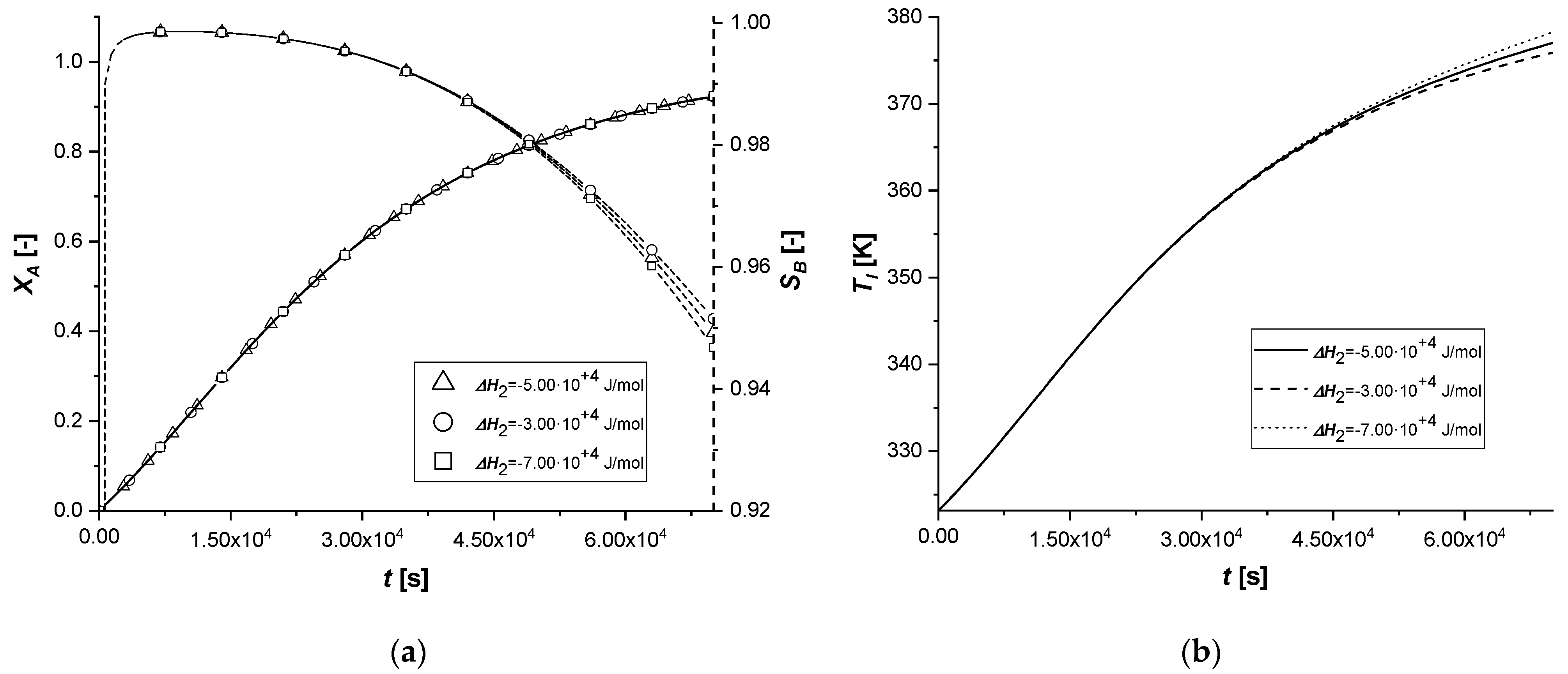
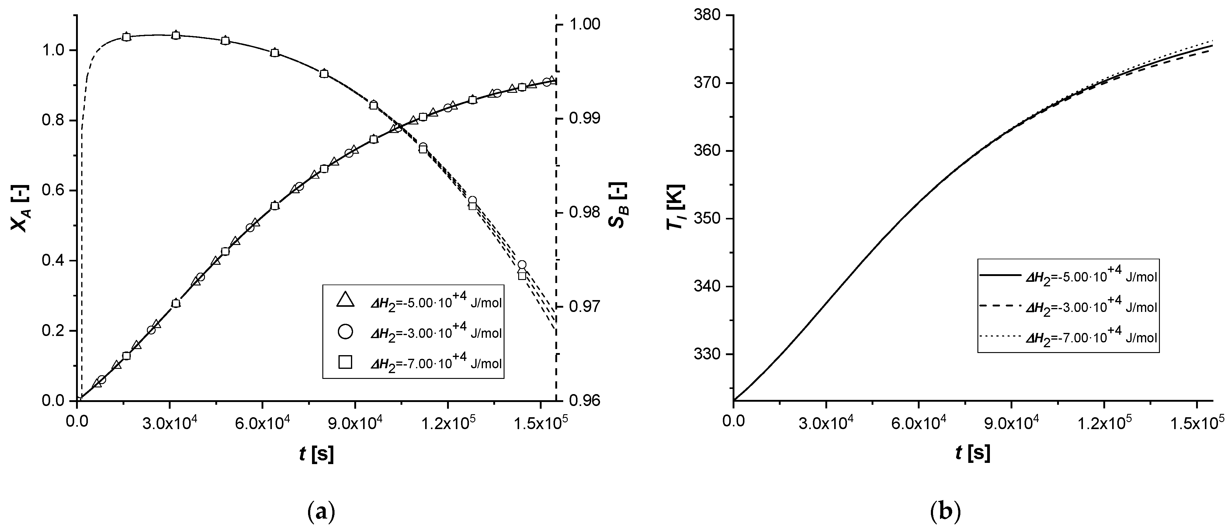
The variation of the enthalpy of the second reaction causes effects similar to those observed in the previous simulations, influencing the reaction rates.
Unlike the ΔH1 case, since the second reaction is slower than the first (kref2 << kref1) and produces C in smaller quantities than B, the energy contribution will certainly be reduced compared to the previous simulations.
The comparison between the solid side and liquid side concentration profiles calculated for all the catalytic cases are reported in Supplementary Materials in Figures S10–S18. The details of each conversion, selectivity, and liquid side temperature profiles are shown in Figure 8, Figure 9 and Figure 10.
As can be seen from Figure 10, the variation of ΔH2 obtained starting from the same values used in the study of ΔH2, led to completely different results. Both the solid-side and liquid-side profiles overlap almost completely in all the cases showing slight deviations from the standard behavior only in the production of C in the EW and EY cases. As anticipated, the energy contribution provided is very limited due to the low concentration of C produced. In cases where the catalytically active phase is positioned in the innermost parts of the particle, the reactive thrust is displayed in a slightly more evident way, but the effect of the parameter remains extremely limited.

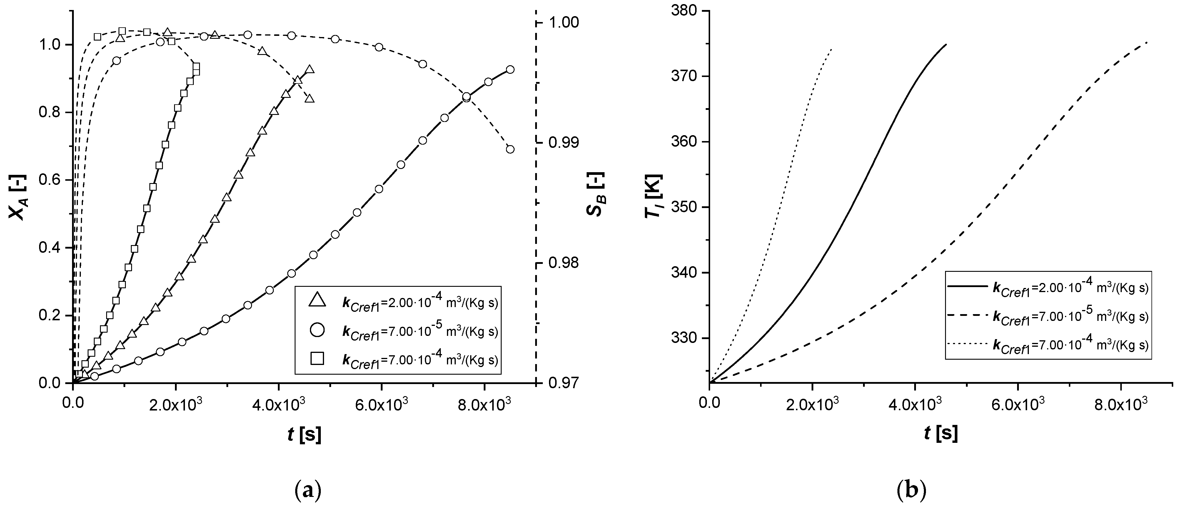
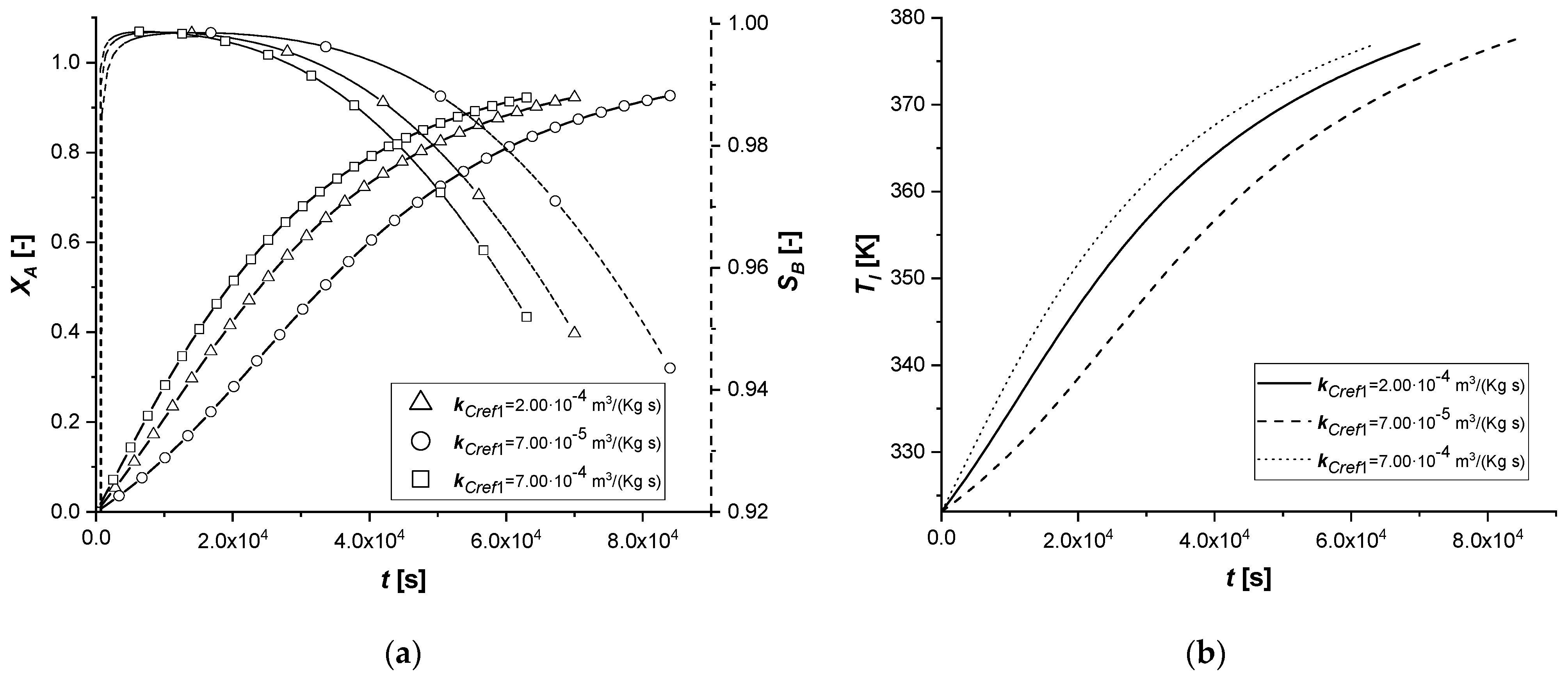
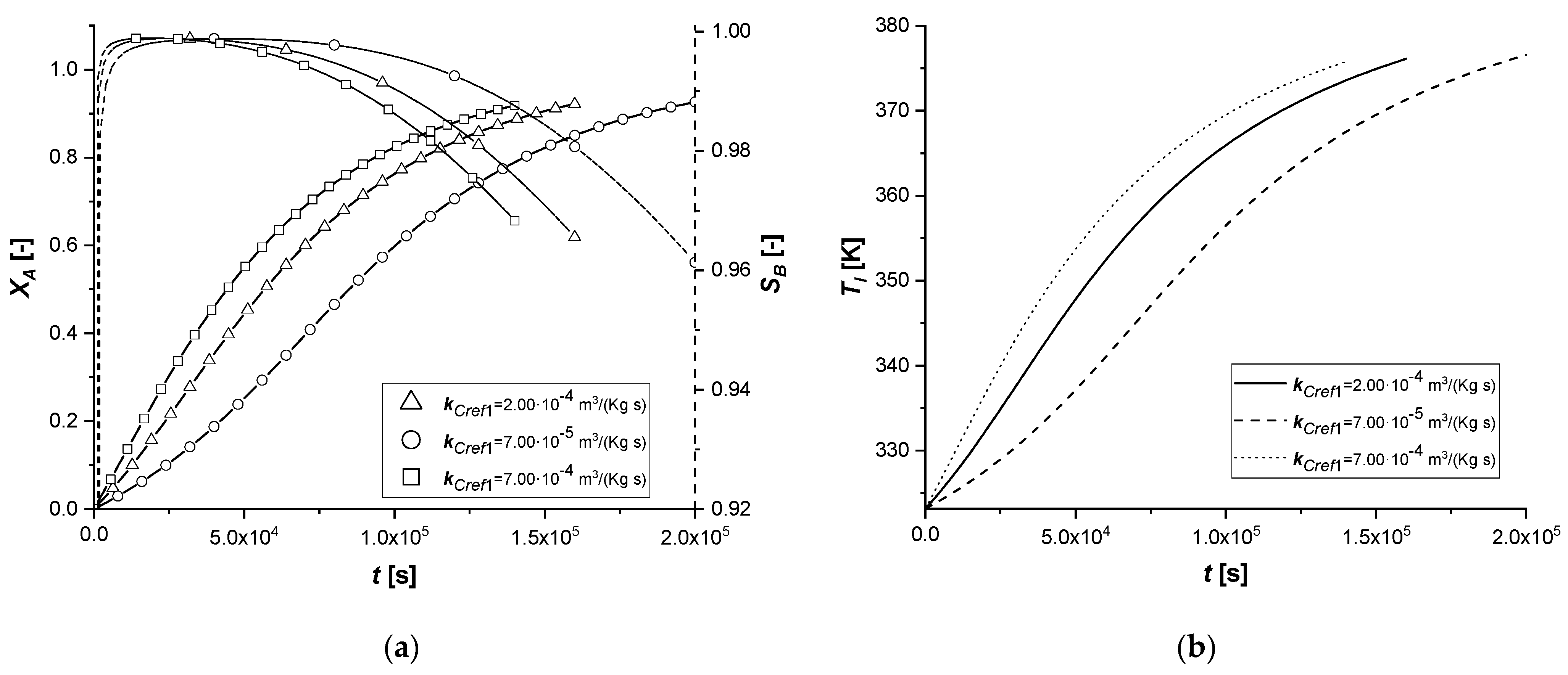
3.2.2. Reaction Rate Constants

The manipulation of the reference kinetic constant of the first reactive process determines the variation of its reaction rate. Consequently, an increase in the amount of reactant diffused in the particle or an improvement in the production of the intermediate can be expected.
The comparison between the solid side and liquid side concentration profiles calculated for all the catalytic cases are reported in Supplementary Materials in Figures S19–S27. The details of each conversion, selectivity, and liquid side temperature profiles are displayed in Figure 11, Figure 12 and Figure 13.
As the kinetic parameter increases, both reactive processes are accelerated. If for the first reaction the increase in the rate is evident, the second receive an improvement due to the high concentration of B, because its kinetics of first order with respect to the intermediate.
It is interesting to note that unlike the first set of enthalpy simulations, the decreasing trend on the liquid side of cBl is not observed in the EW and EY cases. The second chemical reaction is less affected than the ΔH1 study. In these simulations, in the cases of EW and EY, the consumption of A is clearly limited by internal diffusion resistance.
With the consequent decrease of the kinetic constant, the reaction times increase moderately, showing a growth in the production of the by-product C, especially in the ES case.
Also in this study, the use of ES type catalysts can be favored if the desired product is the intermediate one.
The comparison between the solid side and liquid side concentration profiles calculated for all the cases, varying the second-rate constant, are reported in Supplementary Materials in Figures S28–S36. The details of each conversion, selectivity, and liquid side temperature profiles are displayed in Figure 14, Figure 15 and Figure 16.
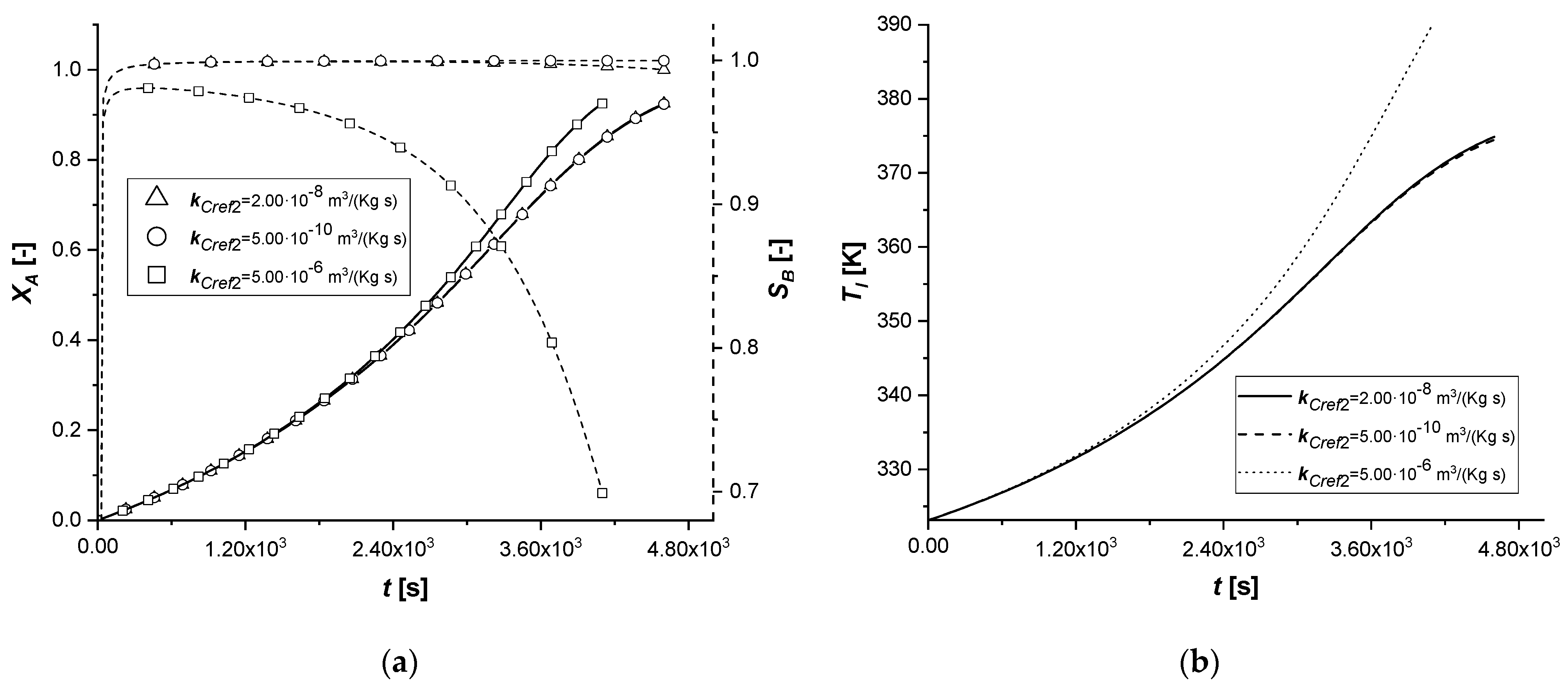
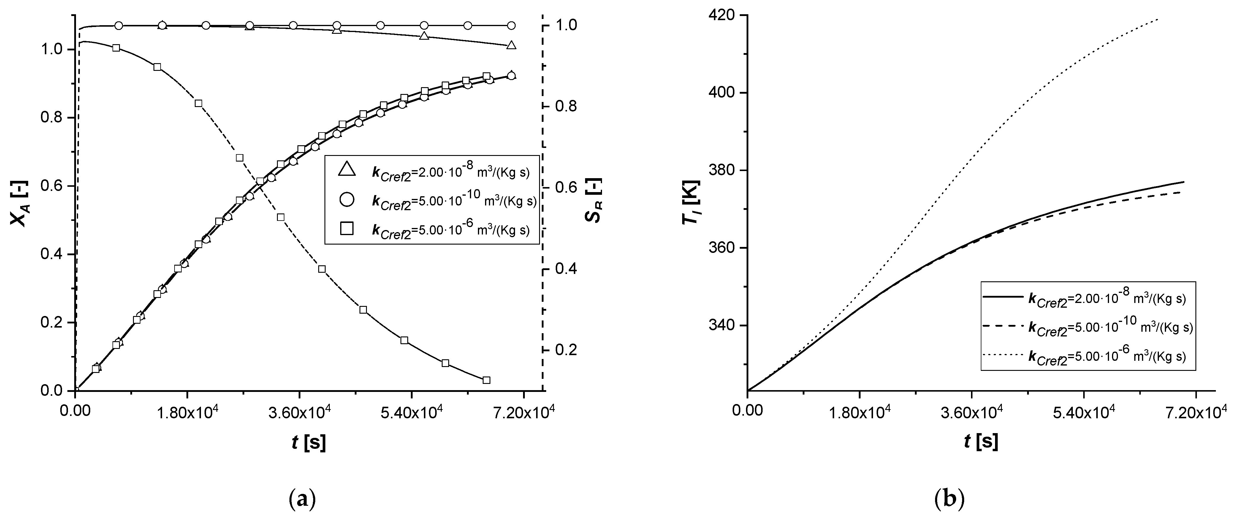
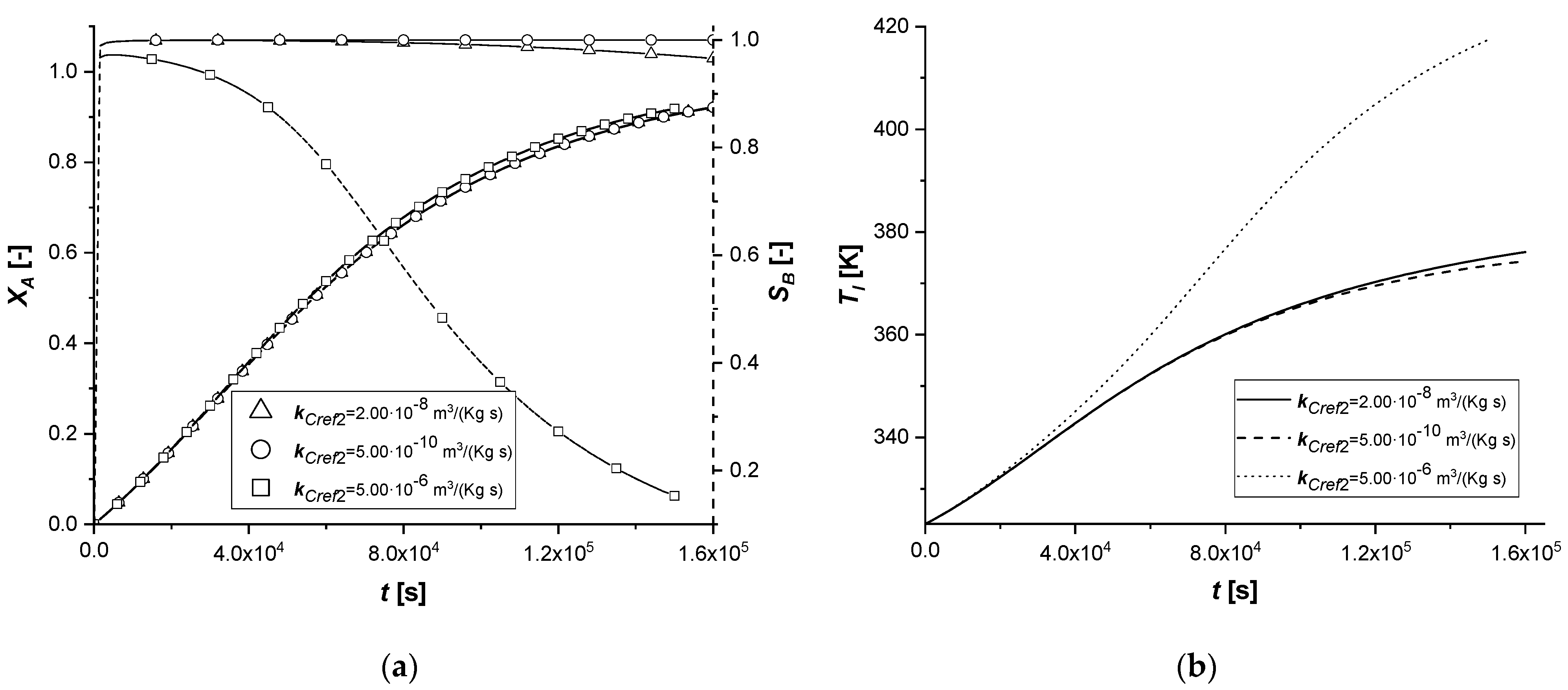
The kinetic parameter, kCref2, is under standard conditions, four orders of magnitude lower than the first chemical reaction; consequently, its further lowering involves a decrease in the quantity of the final product C. In all the cases, it is possible to observe that both the liquid and solid side profiles tend to overlap the reference simulation with small exceptions.
By increasing the parameter and making it comparable with kCref1, it is observed an increase in the production of C. For the first time, there is a beginning of a descending phase in the cBl profile in the ES. In the EW and EY cases the concentration of the intermediate in the liquid is the lowest ever observed, also preventing the accumulation of the component inside the particle.

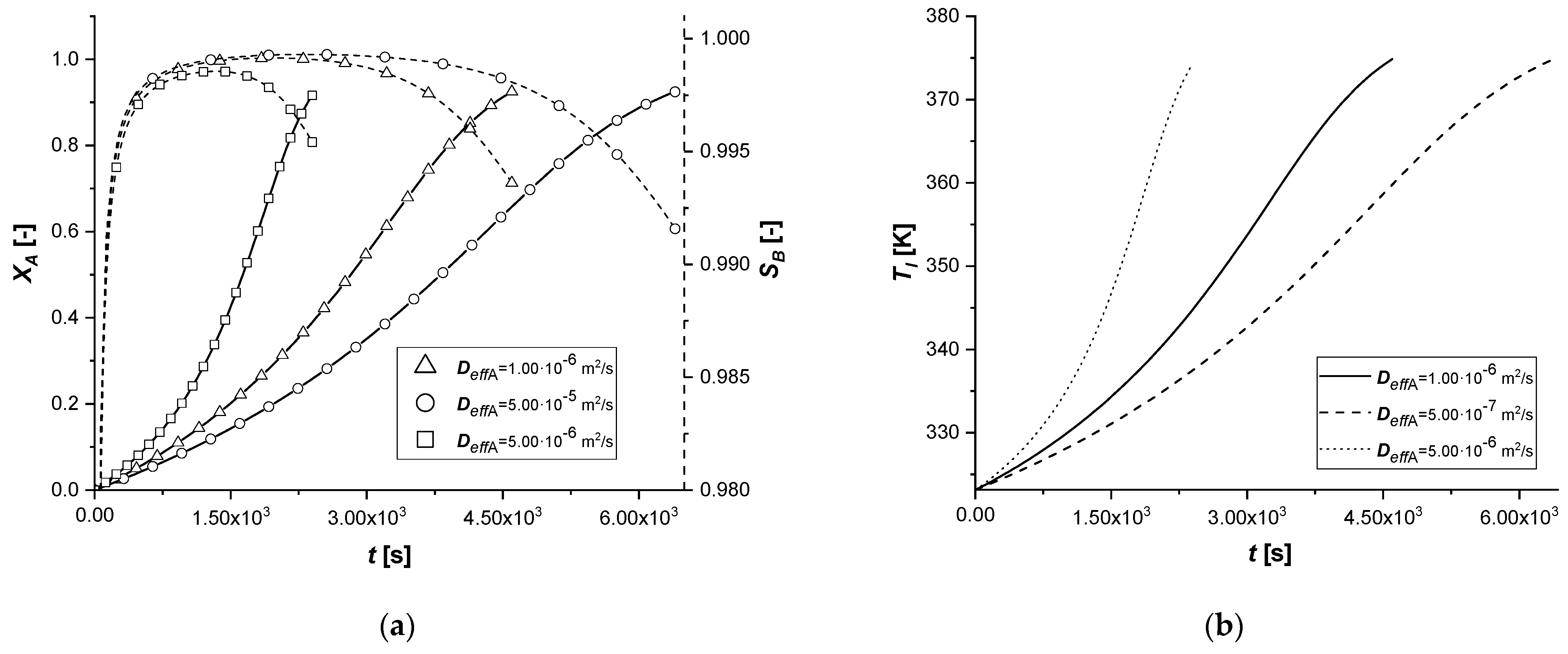
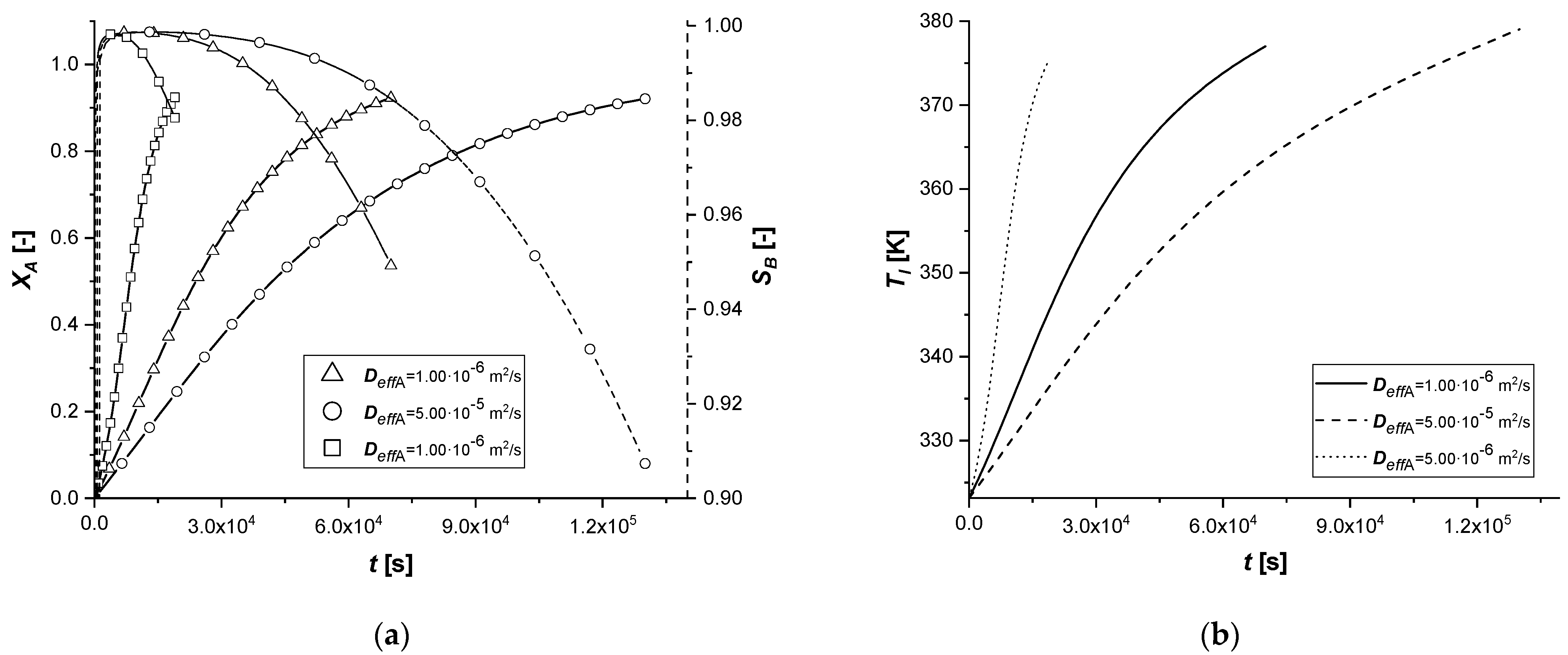
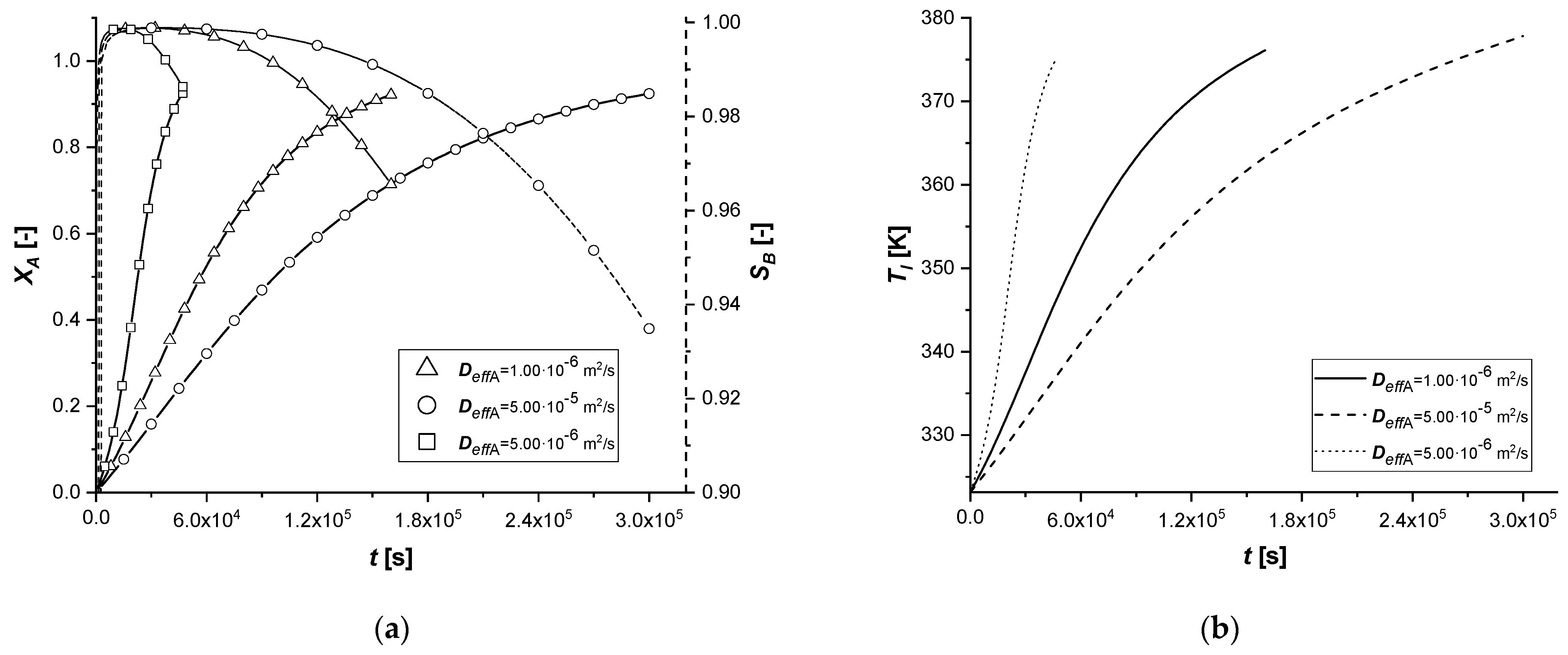
3.2.3. Effective Molecular Diffusivity

The molecular diffusivity coefficient, appearing in the model in the solid-side mass balance, intervenes in the intraparticle mass transport resistance. Therefore, this study focused exclusively on the variation of the diffusive parameter of reagent A.
The comparison between the solid side and liquid side concentration profiles computed for all catalytic cases are reported in Supplementary Materials in Figures S37–S45. The details of each conversion, selectivity, and liquid side temperature profiles, calculated for all catalytic cases, are displayed in Figure 17, Figure 18 and Figure 19.
As can be seen from the results, a modest variation in Deff,A causes significant changes in the concentration profiles of the solid and liquid sides.
In particular, the resulting decrease of the parameter determines an increase in the resistance of intraparticle mass transport of A. It is possible to notice extended reaction times, especially in cases where the catalytic phase is located in the depth of the catalyst.
The increment of Deff,A generates diametrically opposite effects; much faster reactions are observed, due to less diffusion resistance within the solid phase. It is interesting to note that for the reactive process causes, for the first time, the achievement of an intra-particle concentration of the intermediate is higher than 1 mol m−3.
Finally, the amount of the final product cCl obtained is very low when the mass transfer of A is less limiting.

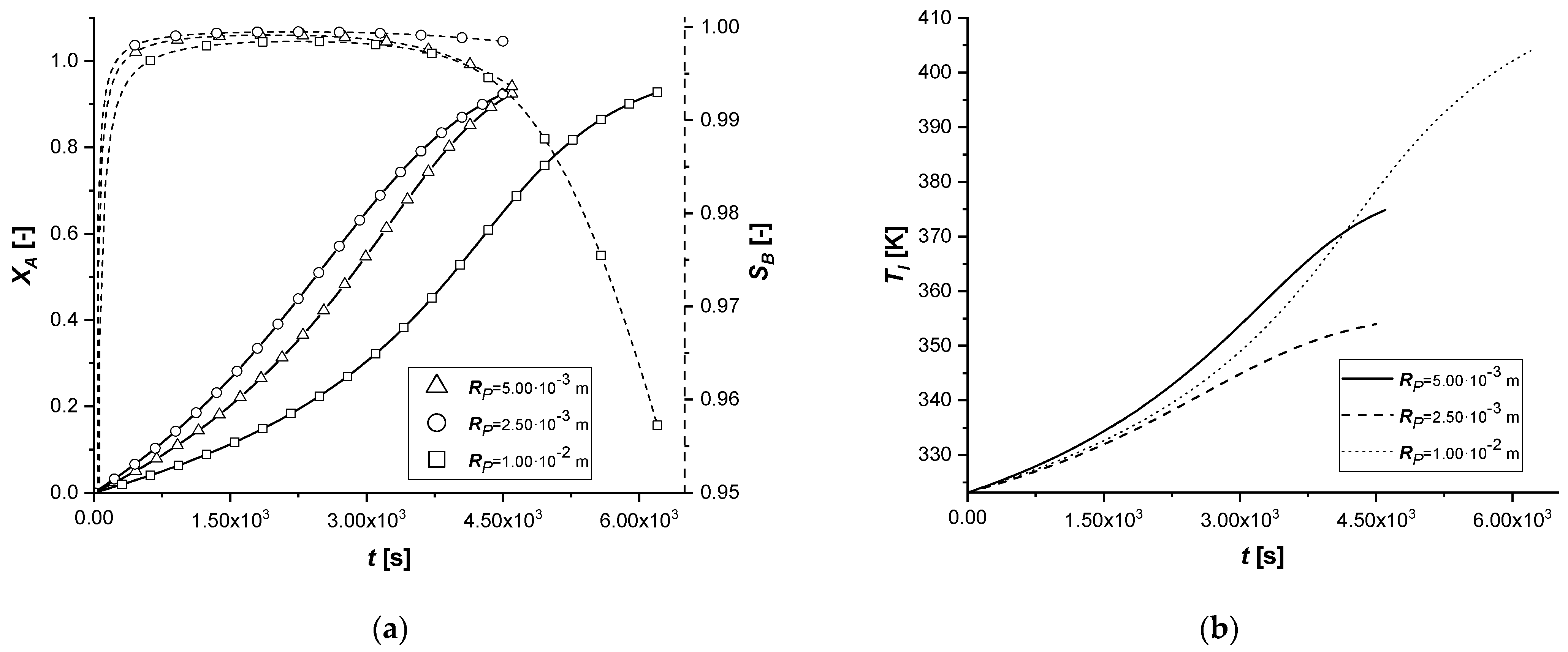
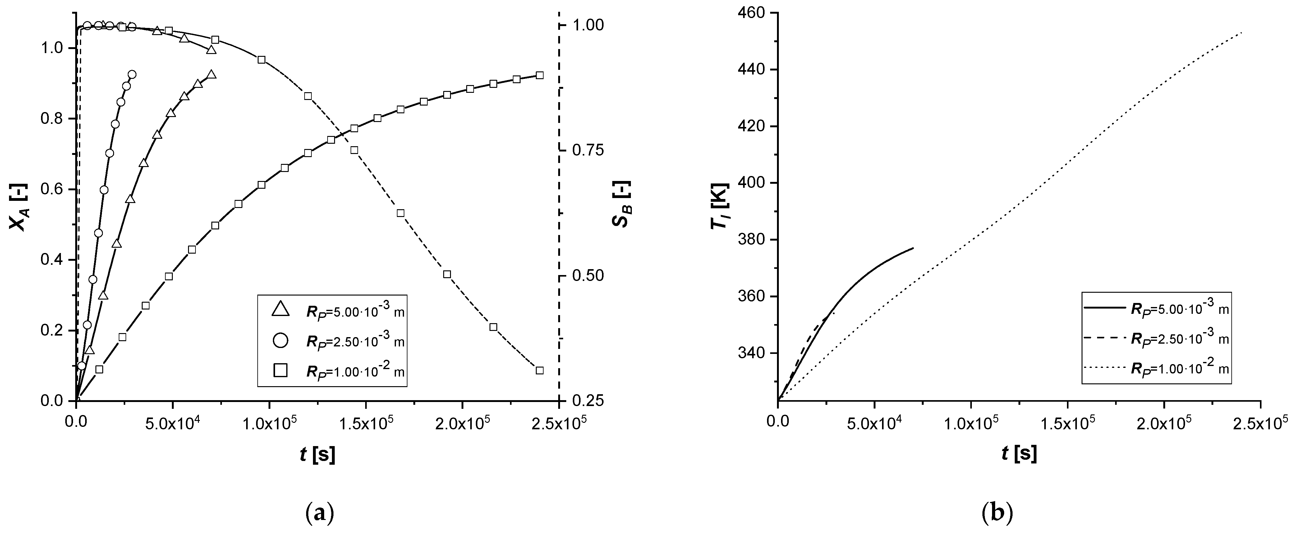
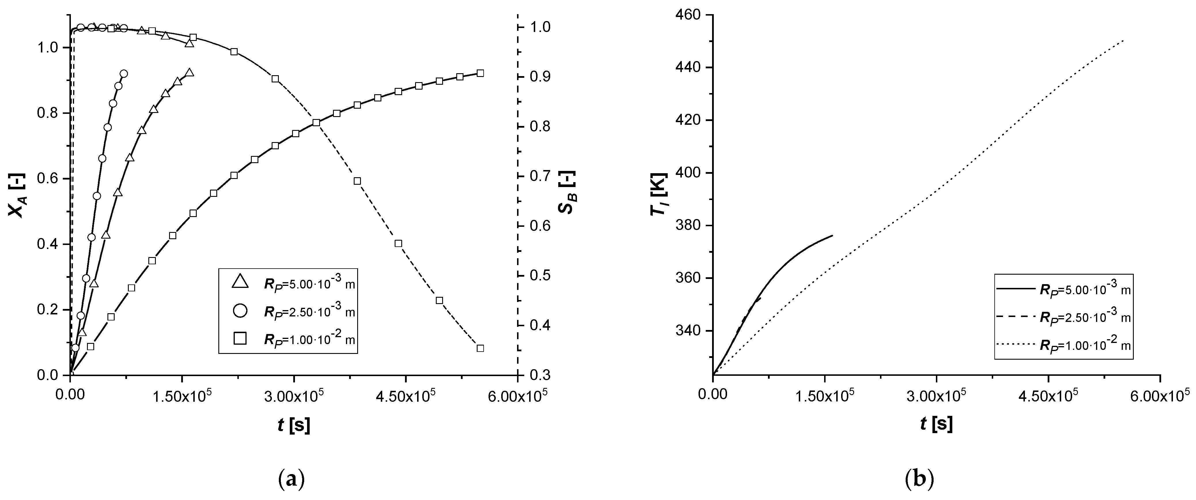
3.2.4. Particle Radius

The effect of the variation of the particle radius in the model is to be found in both mass balances. In particular, RP is placed both in the internal diffusive term, altering the transport resistance, and in the external diffusive term by modifying the contact surface between the two phases, identified in the relationship between the surface of the particle and its volume (asp).
The comparison between the solid side and liquid side concentration profiles calculated for all the catalytic cases are reported in Supplementary Materials in Figures S46–S54. The details of each conversion, selectivity, and liquid side temperature profiles, calculated for all catalytic cases, are displayed in Figure 20, Figure 21 and Figure 22.
Observing the results in the comparison graphs, it can be stated that the response of the model to the variation of RP is opposite to what is visible in the simulations involving Deff,A. It is important to remember that, unlike the previous case, where the effect was focused only on the main reacting species, in these simulations, the effect is related to all the species involved.
In particular, a reduction of the particle size favors the diffusion of the reagent inside it and of the products towards the bulk. This result can be visualized very well due to the short reaction times. With a small radius, the quantity cBl obtained in all cases is very high to the detriment of the by-product.
If the particle size increases, the limitation caused by diffusive internal phenomena becomes even more dominant. In all the cases, a significant increase in the concentration of C is observed. This phenomenon is caused by the difficulty of B, once formed in the catalytic zone, to diffuse backward, accumulating in the solid and promoting the second reaction.
The influence of RP in the liquid side balance is less evident than that observed in the solid side, being the external diffusive term much less sensitive to its small alterations.
It can be assumed that the use of catalysts with a small particle radius favors the production of the reaction intermediate.

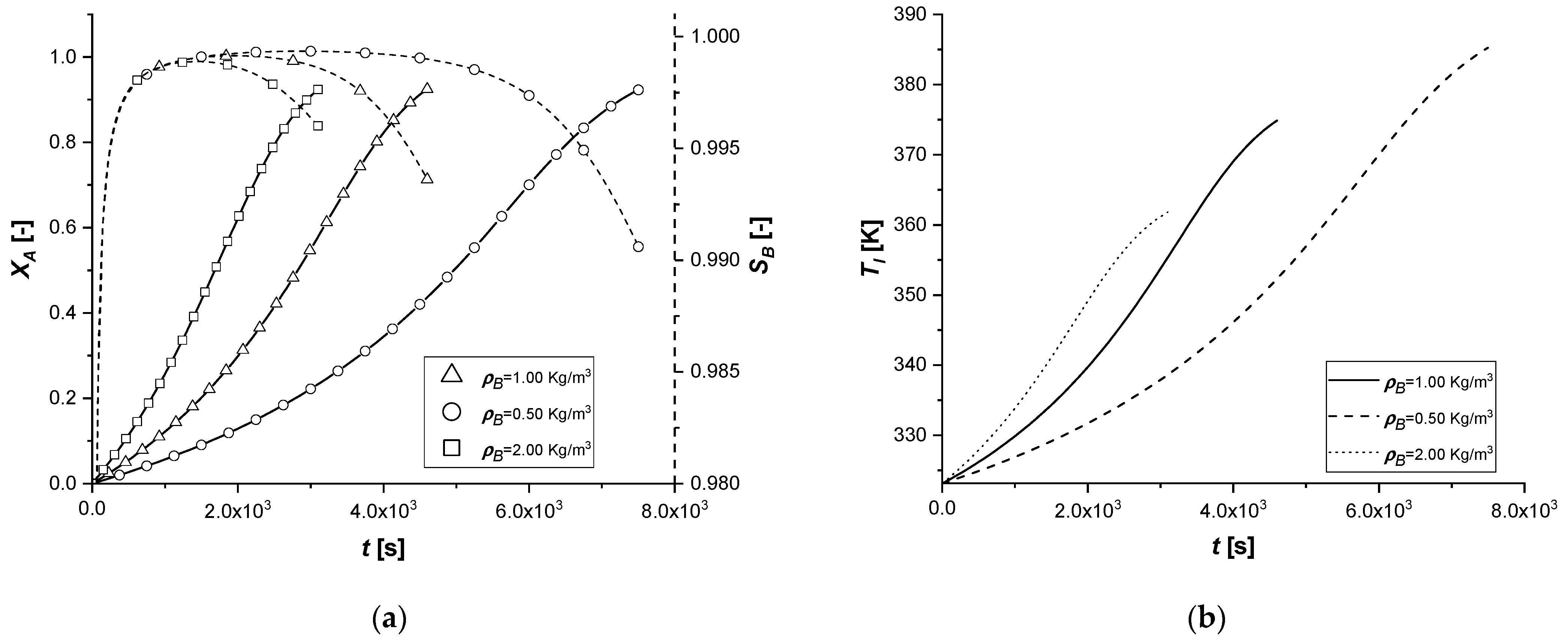
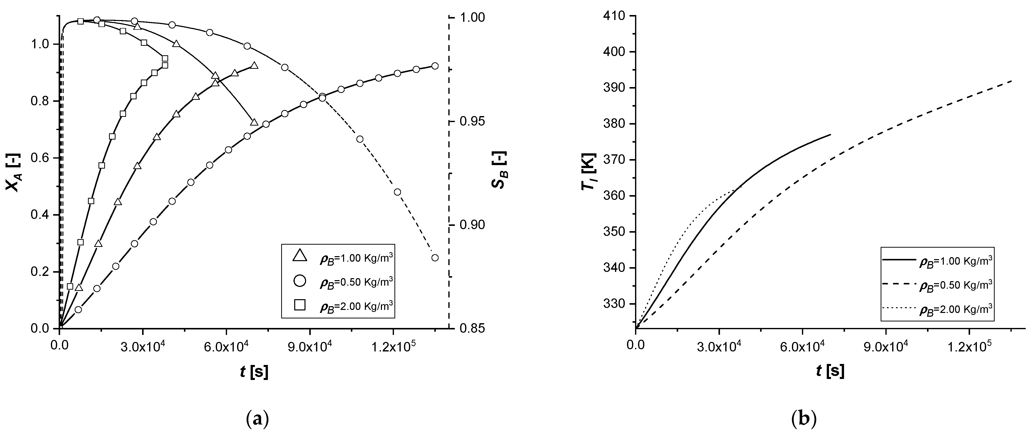
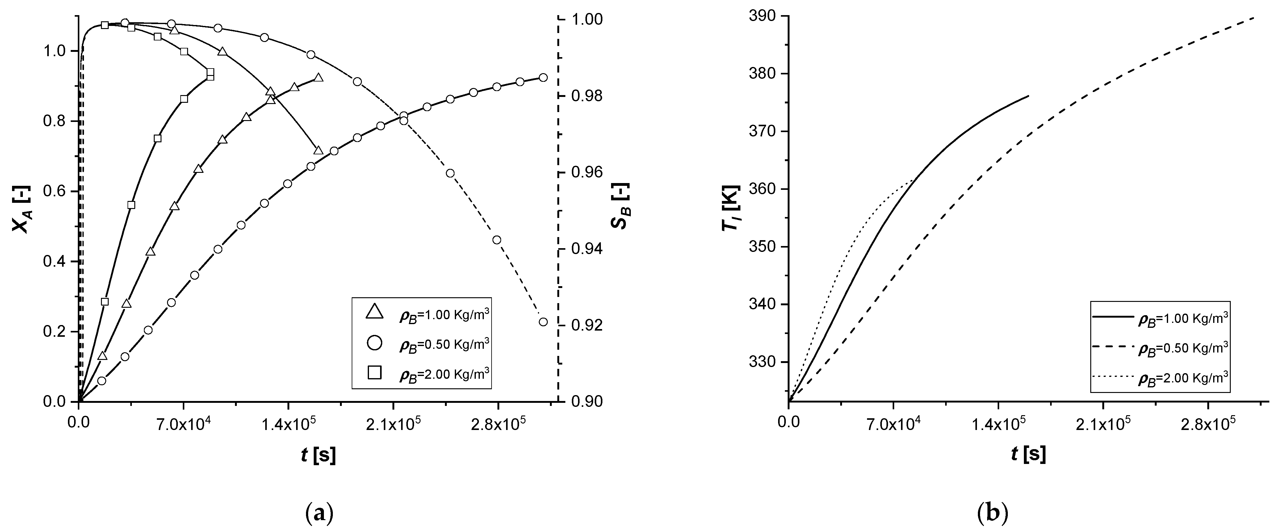
3.2.5. Catalyst Bulk Density

The consequent alteration of ρP, for the same particle radius, consists in a modification of the mass of catalyst present in the reactive system. This parameter directly affects the generative terms of intraparticle mass and energy balances. Finally, it also intervenes in the liquid side mass balance in the term ε.
The comparison between the solid side and liquid side concentration profiles calculated for all the catalytic cases are reported in Supplementary Materials in Figures S55–S63. The details of each conversion, selectivity, and liquid side temperature profiles, calculated for all catalytic cases, are shown in Figure 23, Figure 24 and Figure 25.
The results obtained in the comparison graphs show that the decrease in ρP entails a slowdown in the entire chemical process due to the lower contribution of the generative terms. In fact, the accumulation of reagent A in the intraparticle profiles is observed, unlike the simulations with higher density values.
The increase in the quantity of catalyst accelerates all reactive cases and determines a lower production of by-product C in the reaction times.
It is important to consider that the alteration of this coefficient emphasizes important characteristics of the system: despite the correlation with both generative terms of mass, the gap between the two reactions tends to grow as the parameter increases.

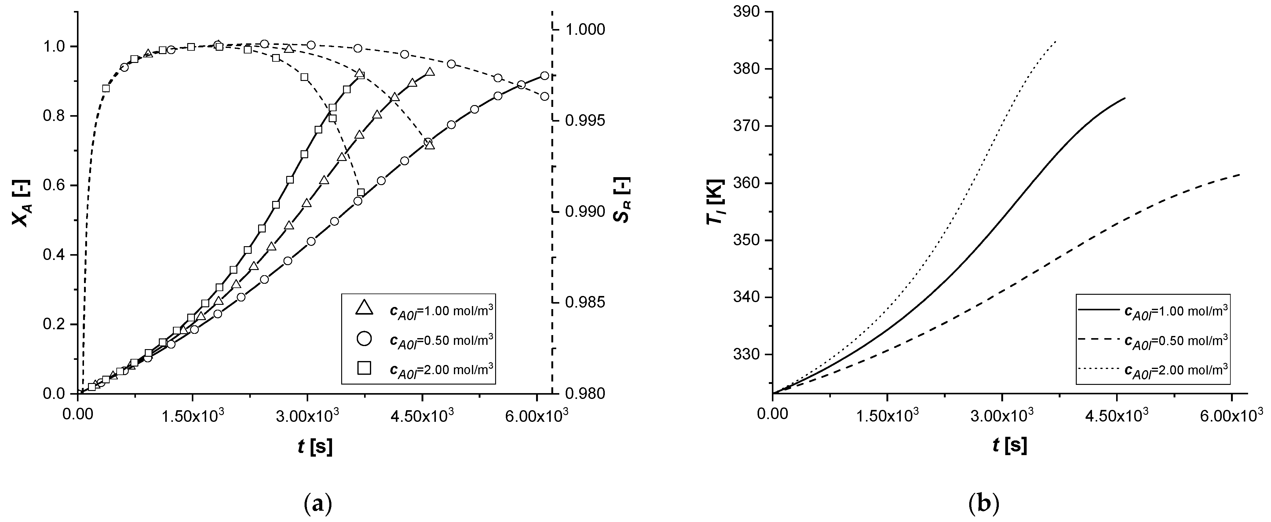
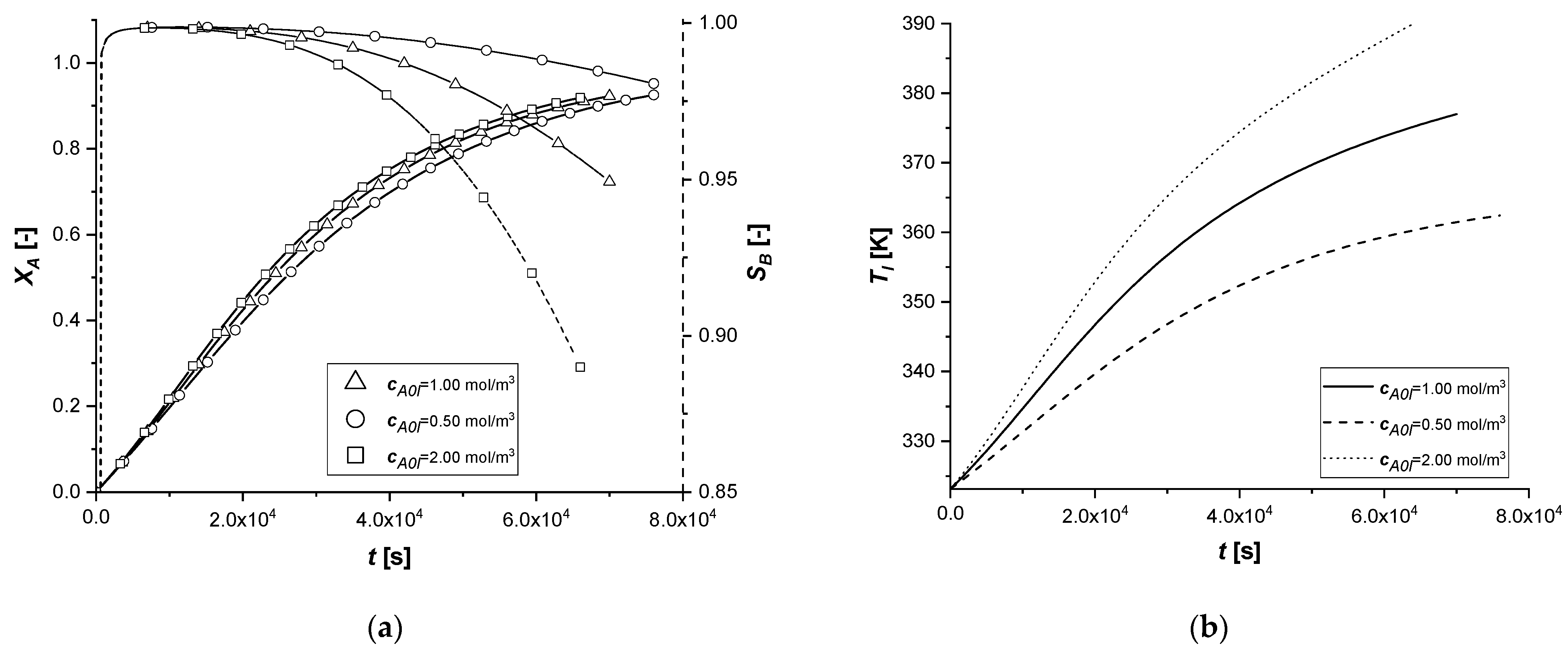
3.2.6. Initial Bulk Concentration of A

The change in the initial concentration of A in the liquid phase affects the model through the mass and energy balances.
In the absence of chemical reactions in the liquid phase, the parameter mainly influences the gradient at the liquid–solid interface.
Furthermore, for an exothermic reaction, the quantity of reactant available determines the amount of energy released during the reaction and consequently the operating temperature, which affects the main kinetic parameters.
The comparison between the solid and liquid side concentration profiles calculated for all the catalytic cases are reported in Supplementary Materials in Figures S64–S72. The details of each conversion, selectivity, and liquid side temperature profiles, calculated for all catalytic cases, are shown in Figure 26, Figure 27 and Figure 28.
The results demonstrate how the chemical process behaves consistently with respect to the decrease or increase of the parameter cA0,l. In all the cases, the reaction times, for obtaining the desired conversion, are similarly decreasing moderately with the increment of the available reagent. ES is the catalytic case most influenced by the parameter, probably due to the immediate availability of the catalytic zone, unlike the other two cases.
Finally, it is interesting to notice, again in the case of the ES, how the slope of the intraparticle profiles of component A changes at the entrance to the solid (x = 1) due to the different concentration gradients at the interface.

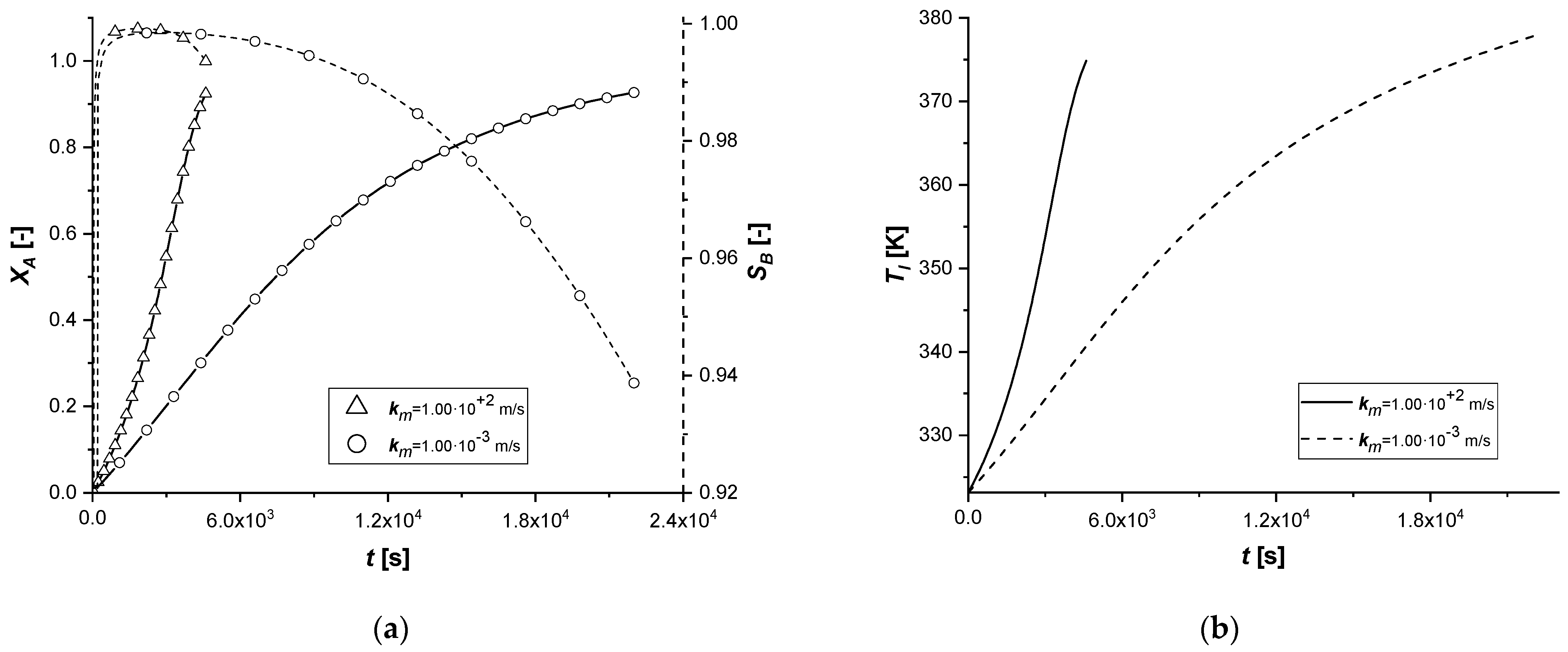
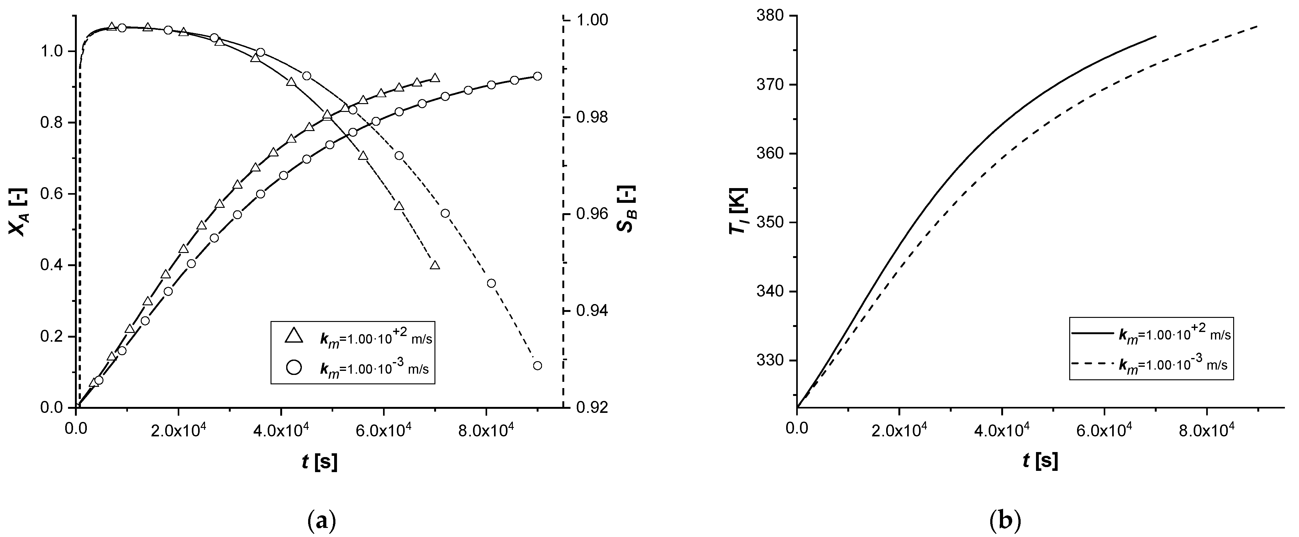
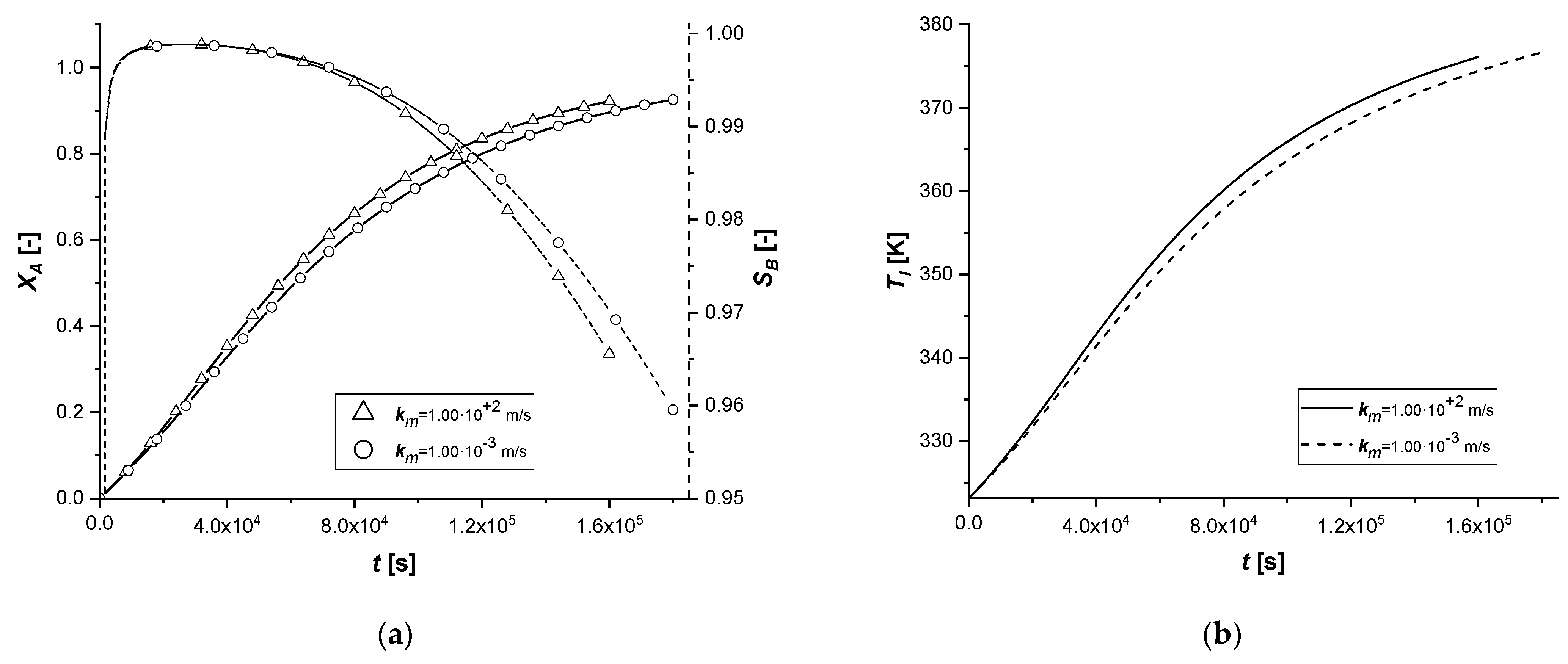
3.2.7. Liquid–Solid Mass Transfer Coefficient

The liquid–solid mass transfer coefficient under standard conditions is sufficiently high to keep the external diffusion effects negligible. In this study, the response of the system was evaluated by assuming that the resistance to transport on the surface of the catalytic particle becomes influential in the reactive process.
The comparison between the solid side and liquid side concentration profiles calculated for all the catalytic cases are reported in Supplementary Materials in Figures S73–S81. The details of each conversion, selectivity, and liquid side temperature profiles, calculated for all catalytic cases, are shown in Figure 29, Figure 30 and Figure 31.
From the comparison graphs, it is possible to observe that, by considerably reducing the numerical value of the parameter km, the influence on the ES catalyst seems to be more significant than in the other two cases.
In fact, if for EW and EY the limiting process remains the internal diffusive one, in the first catalytic case, extended reaction times are observed. Furthermore, for the first time, it is possible to observe for the ES a concentration cCl at the end of the reaction, comparable if not higher than the other two cases.
In order to avoid the increase of external diffusion resistance, it is advisable to use high stirring rates in batch reactors. It is known that as the stirring rate increases, the thickness of the film of stagnant liquid at the interface between the phases diminishes, suppressing the mass transfer resistance.

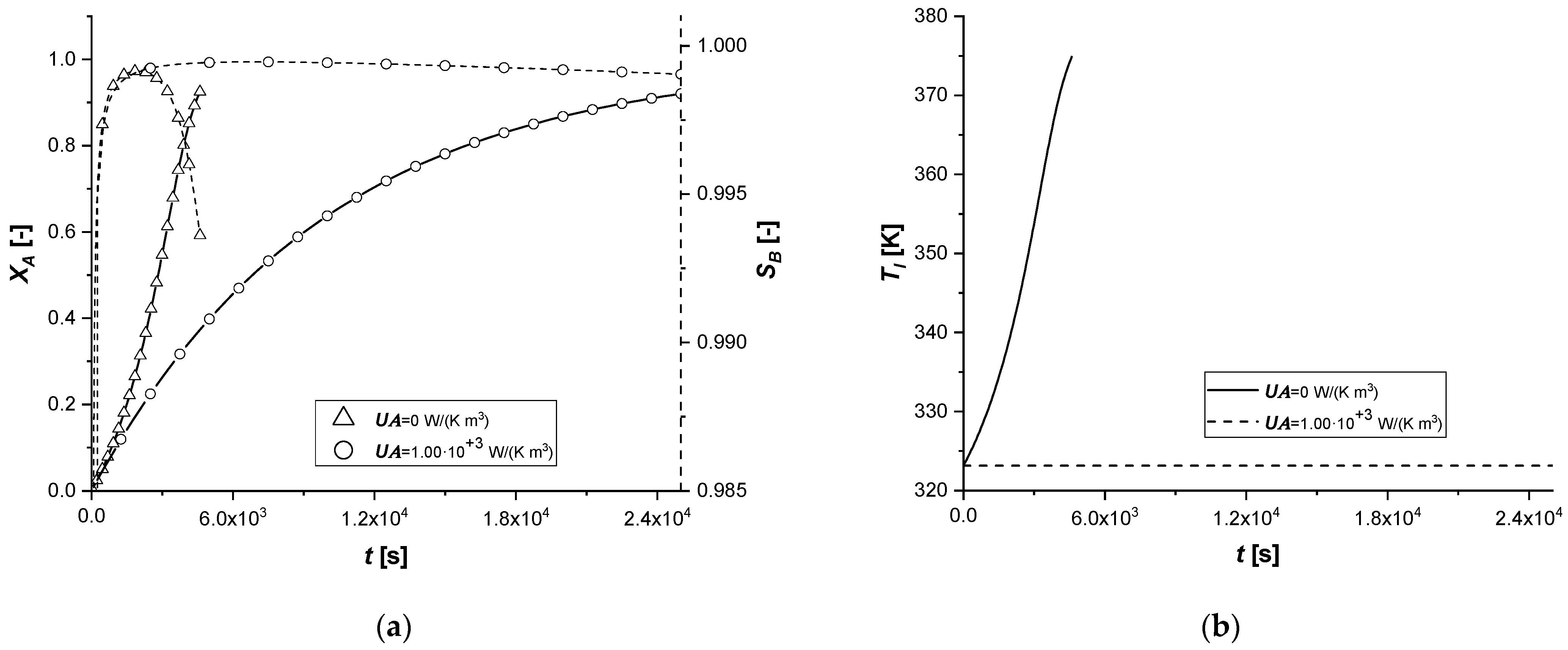
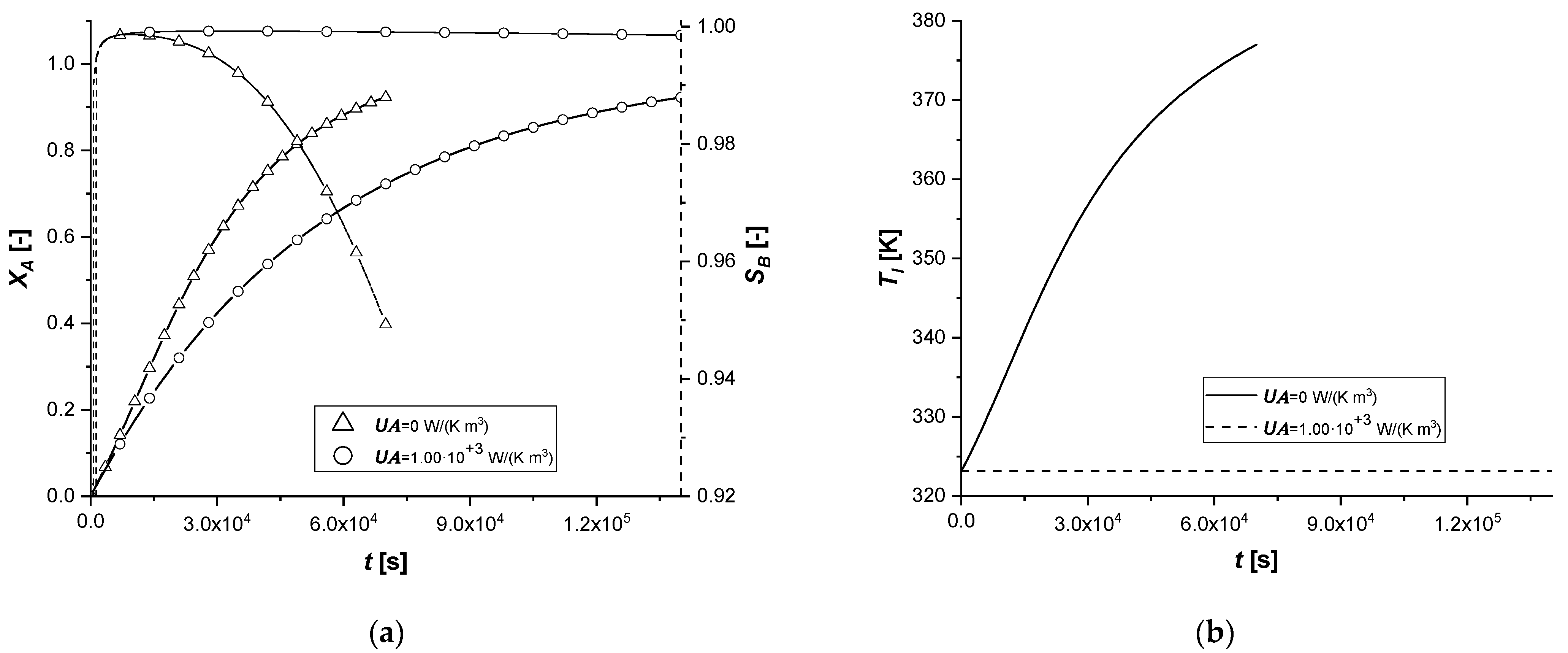
3.2.8. External Thermal Resistance

This parametric study was conducted by evaluating the response of the model in the presence of an energy exchange term with the external environment, simulating the dissipation of a part of the energy deriving from the chemical reaction.
The comparison between the solid side and liquid side concentration profiles calculated for all the catalytic cases are reported in Supplementary Materials in Figures S82–S90. The details of each conversion, selectivity, and liquid side temperature profiles, calculated for all catalytic cases, are shown in Figure 32, Figure 33 and Figure 34.
The results confirm that the presence of an energy dissipative term causes a slowdown of all chemical processes, as a consequence of the lowering of the system temperature compared to the reference case.
In fact, the intraparticle concentration cAs profiles show a considerable accumulation of the reagent given the low reaction rates, which are functions of operation temperature. Finally, it is interesting to notice that when the desired conversion is achieved, the bulk concentration of the final product C is extremely low in all the cases.

4. Conclusions

In this work, the influence of several parameters on three different catalytic systems was investigated in order to obtain a high selectivity of the intermediate product of a consecutive reaction system A→B→C in an adiabatic batch reactor. These systems are distinguished from each other by the different distribution of the active phase inside the catalyst particle. In the mathematical model, active phase distribution equations and appropriate mass and energy balances were implemented. Simulations of concentration profiles of all the components in the solid and liquid phases, the temperature profiles, the reactant conversion, and the product selectivity for each case were obtained. The comparison between the different catalysts, varying the most influential parameters, revealed that the catalysts with active phase distribution egg white and egg yolk always show selectivity, to the desired intermediate product, which is lower or, in a few case studies, comparable to that of the egg shell, which proves to be the catalyst that tends to maximize the selectivity of B.
The implemented model can be easily adapted for a study in more complex systems, and, for continuous reactor systems, possibly focusing the attention on the catalyst whose active phase distribution allows to maximize the selectivity of the desired product. Thus, the presented modeling approach shows the opportunity to optimize a NUD heterogeneous catalyst placed in a specific reactor unit (e.g., packed bed, continuous stirred tank, fluidized bed reactor) for a chosen chemical system, leading to higher reactant conversion, higher product selectivity with the lowest catalyst cost.

Supplementary Materials

Author Contributions

Conceptualization, V.R. and T.S.; methodology, E.S., V.R.; software, E.S.; validation, E.S.; formal analysis, E.S., V.R., T.S., R.T.; investigation, E.S.; data curation, E.S., V.R.; writing—original draft preparation, E.S.; writing—review and editing, E.S., V.R., T.S., R.T., M.D.S.; supervision, T.S., R.T., M.D.S.; project administration, V.R. All authors have read and agreed to the published version of the manuscript.

Funding

This research received no external funding.

Institutional Review Board Statement

Not applicable.

Informed Consent Statement

Not applicable.

Data Availability Statement

Data is contained within the article or Supplementary Materials.

Acknowledgments

Luca Mastroianni is acknowledged for the help given to the present study.

Conflicts of Interest

Authors declare no conflicts of interest.

Abbreviations

ESEgg Shell
EWEgg White
EYEgg Yolk
lLiquid domain
PParticle
sSolid domain
Symbols
a1Inflection point for Egg Shell profile [-]
a2Inflection point for Egg Yolk profile [-]
a31Inflection point 1 for Egg White profile [-]
a32Inflection point 2 for Egg White profile [-]
aspSpecific surface area [m2/m3]
bSmoothing factor [-]
ci0,lInitial concentration in liquid phase [mol/m3]
ci,lConcentration in liquid phase [mol/m3]
ci,sConcentration in solid phase [mol/m3]
cp,iSpecific heat of the fluid component [J/(mol K)]
cp,lSpecific heat of the liquid phase [J/(mol K)]
cp,PSpecific heat of the particle [J/(mol K)]
Deff,iEffective molecular diffusivity [m2/s]
EajActivation energy of reaction j [J/mol]
hThermal resistance solid-liquid interface [W/(m2 K)]
kjCatalytic rate constant [m3/(kg s)]
krefjCatalytic reference rate constant [m3/(kg s)]
kmFluid–solid mass transfer coefficient [m/s]
kT,lFluid heat conductivity [W/(m K)]
kT,PParticle heat conductivity batch reactor [W/(m K)]
MWiMolecular weight [g/mol]
NNumber of component [-]
rjCatalytic reaction rate [mol/(kg s)]
RgIdeal gas constant [J/(K mol)]
RPParticle radius [m]
sShape factor [-]
SBSelectivity B [-]
tTime [s]
TjExternal temperature [K]
TlLiquid phase temperature [K]
TsSolid phase temperature [K]
TrefReference temperature [K]
UAExternal thermal resistance [W/(m2 K)]
xDimensionless radial coordinate of the spherical particle [–]
XAConversion degree of A [–]
yBYield B [-]
ΔrHjReaction enthalpy [J/mol]
εVolumetric ratio between the solid and the liquid phases batch reactor [-]
εpCatalyst porosity [-]
ηEfficiency reaction [-]
νijStoichiometric matrix [-]
ρiComponent density [kg/m3]
ρlLiquid phase density [kg/m3]
ρPParticle density [kg/m3]
ρBulkCatalyst bulk density (mass of catalyst/volume) [kg/m3]
ΩkDistribution function [-]
Subscripts
AInitial reagent
BIntermediate reaction component
Cfinal reaction product
iComponent
jReaction
kDistribution type
refReference

References

  1. Russo, V.; Santacesaria, E.; Tesser, R.; Turco, R.; Vitiello, R.; Di Serio, M. Validation of the kinetics of the Hydrogen Peroxide Propene Oxide (HPPO) process in a dynamic Continuous Stirred Tank Reactor. Ind. Eng. Chem. Res. 2018, 57, 16201–16208. [Google Scholar] [CrossRef]
  2. Gavriilidis, A.; Varma, A. Optimal catalyst activity profiles in pellets: 9. Study of ethylene epoxidation. AIChE J. 1992, 38, 291–296. [Google Scholar] [CrossRef]
  3. Johnson, D.L.; Verykios, X. Selectivity enhancement in ethylene oxidation employing partially impregnated catalysts. J. Catal. 1983, 79, 156–163. [Google Scholar] [CrossRef]
  4. Russo, V.; Kilpiö, T.; Hernandez, J.C.; Di Serio, M.; Salmi, T.O. Modelling of microreactors for ethylene epoxidation and total oxidation. Chem. Eng. Sci. 2015, 134, 563–571. [Google Scholar] [CrossRef]
  5. Russo, V.; Mastroianni, L.; Tesser, R.; Salmi, T.; Di Serio, M. Intraparticle Modeling of Non-Uniform Active Phase Distribution Catalyst. ChemEngineering 2020, 4, 24. [Google Scholar] [CrossRef] [Green Version]
  6. Hwang, S.; Linke, P.; Smith, R. Heterogeneous catalytic reactor design with optimum temperature profile II: Application of non-uniform catalyst. Chem. Eng. Sci. 2004, 59, 4245–4260. [Google Scholar] [CrossRef]
  7. Komiyama, M. Design and Preparation of Impregnated Catalysts. Catal. Rev. 1985, 27, 341–372. [Google Scholar] [CrossRef]
  8. Morbidelli, M.; Gavriilides, A.; Varma, A. Optimal Distribution of Catalyst in Pellets, Reactors and Membranes; Cambridge University Press: Cambridge, UK, 2001. [Google Scholar]
  9. Mazdidi, S.K.; Sadeghi, M.T.; Marvast, M.A. Optimization of Fischer-Tropsch Process in a Fixed-Bed Reactor Using Non-uniform Catalysts. Chem. Eng. Technol. 2012, 36, 62–72. [Google Scholar] [CrossRef]
  10. Tesser, R.; Russo, V. Advanced Reactor Modelling with MATLAB; De Gruyter: Berlin, Germany, 2021. [Google Scholar]
  11. Geankoplis, C.J. Transport Processes and Separation Process Principles, 4th ed.; Pearson College Div: London, UK, 2003. [Google Scholar]
  12. Salmi, T.; Mikkola, J.P.; Wärnå, J. Chemical Reaction Engineering and Reactor Technology, 2nd ed.; CRC Press: Boca Raton, FL, USA, 2019. [Google Scholar]
  13. Rädler, J. Smoots Transition between Functions with Tanh(). Available online: https://www.j-raedler.de/2010/10/smooth-transition-between-functions-with-tanh/ (accessed on 8 July 2021).
  14. Process System Enterprise. Available online: www.psenterprise.com (accessed on 8 July 2021).
Figure 1. Intraparticle profiles for ES catalyst. Calculated profiles for: cA (a), cB (b), cC (c) and Ts (d). Color-bar of each plot is located on the right-hand-side.
Chemengineering 05 00038 g001aChemengineering 05 00038 g001b
Figure 2. Intraparticle profiles for EW catalyst. Calculated profiles for: cA (a), cB (b), cC (c) and Ts (d). Color-bar of each plot is located on the right-hand-side.
Chemengineering 05 00038 g002
Figure 3. Intraparticle profiles for EY catalyst. Calculated profiles for: cA (a), cB (b), cC (c), and Ts (d). Color-bar of each plot is located on the right-hand-side.
Chemengineering 05 00038 g003
Figure 4. (a) Bulk profiles over time for ES, EW, and EY. Calculated profiles for: XA and SB. (b) Bulk profiles over time for EY, EW, and EY. Calculated profiles for: Tl. (c) Catalytic effectiveness factor profiles over time for ES, EW, and EY.
Chemengineering 05 00038 g004
Figure 5. ES ΔrH1 investigation. (a) Bulk profiles over time of XA and SB. (b) Bulk profile of Tl over time.
Chemengineering 05 00038 g005
Figure 6. EW ΔrH1 investigation. (a) Bulk profiles over time of XA and SB. (b) Bulk profile of Tl over time.
Chemengineering 05 00038 g006
Figure 7. EY ΔrH1 investigation. (a) Bulk profiles over time of XA and SB. (b) Bulk profile of Tl over time.
Chemengineering 05 00038 g007
Figure 8. ES ΔrH2 investigation. (a) Bulk profiles over time of XA and SB. (b) Bulk profile of Tl over time.
Chemengineering 05 00038 g008
Figure 9. EW ΔrH2 investigation. (a) Bulk profiles over time of XA and SB. (b) Bulk profile of Tl over time.
Chemengineering 05 00038 g009
Figure 10. EY ΔrH2 investigation. (a) Bulk profiles over time of XA and SB. (b) Bulk profile of Tl over time.
Chemengineering 05 00038 g010
Figure 11. ES kCref1 investigation. (a) Bulk profiles over time of XA and SB. (b) Bulk profile of Tl over time.
Chemengineering 05 00038 g011
Figure 12. EW kCref1 investigation. (a) Bulk profiles over time of XA and SB. (b) Bulk profile of Tl over time.
Chemengineering 05 00038 g012
Figure 13. EY kCref1 investigation. (a) Bulk profiles over time of XA and SB. (b) Bulk profile of Tl over time.
Chemengineering 05 00038 g013
Figure 14. ES kCref2 investigation. (a) Bulk profiles over time of XA and SB. (b) Bulk profile of Tl over time.
Chemengineering 05 00038 g014
Figure 15. EW kCref2 investigation. (a) Bulk profiles over time of XA and SB. (b) Bulk profile of Tl over time.
Chemengineering 05 00038 g015
Figure 16. EY kCref2 investigation. (a) Bulk profiles over time of XA and SB. (b) Bulk profile of Tl over time.
Chemengineering 05 00038 g016
Figure 17. ES Deff,A investigation. (a) Bulk profiles over time of XA and SB. (b) Bulk profile of Tl over time.
Chemengineering 05 00038 g017
Figure 18. EW Deff,A investigation. (a) Bulk profiles over time of XA and SB. (b) Bulk profile of Tl over time.
Chemengineering 05 00038 g018
Figure 19. EY Deff,A investigation. (a) Bulk profiles over time of XA and SB. (b) Bulk profile of Tl over time.
Chemengineering 05 00038 g019
Figure 20. ES RP investigation. (a) Bulk profiles over time of XA and SB. (b) Bulk profile of Tl over time.
Chemengineering 05 00038 g020
Figure 21. EW RP investigation. (a) Bulk profiles over time of XA and SB. (b) Bulk profile of Tl over time.
Chemengineering 05 00038 g021
Figure 22. EY RP investigation. (a) Bulk profiles over time of XA and SB. (b) Bulk profile of Tl over time.
Chemengineering 05 00038 g022
Figure 23. ES ρP investigation. (a) Bulk profiles over time of XA and SB. (b) Bulk profile of Tl over time.
Chemengineering 05 00038 g023
Figure 24. EW ρP investigation. (a) Bulk profiles over time of XA and SB. (b) Bulk profile of Tl over time.
Chemengineering 05 00038 g024
Figure 25. EY ρP investigation. (a) Bulk profiles over time of XA and SB. (b) Bulk profile of Tl over time.
Chemengineering 05 00038 g025
Figure 26. ES cA0,l investigation. (a) Bulk profiles over time of XA and SB. (b) Bulk profile of Tl over time.
Chemengineering 05 00038 g026
Figure 27. EW cA0,l investigation. (a) Bulk profiles over time of XA and SB. (b) Bulk profile of Tl over time.
Chemengineering 05 00038 g027
Figure 28. EY cA0,l investigation. (a) Bulk profiles over time of XA and SB. (b) Bulk profile of Tl over time.
Chemengineering 05 00038 g028
Figure 29. ES km investigation. (a) Bulk profiles over time of XA and SB. (b) Bulk profile of Tl over time.
Chemengineering 05 00038 g029
Figure 30. EW km investigation. (a) Bulk profiles over time of XA and SB. (b) Bulk profile of Tl over time.
Chemengineering 05 00038 g030
Figure 31. EY km investigation. (a) Bulk profiles over time of XA and SB. (b) Bulk profile of Tl over time.
Chemengineering 05 00038 g031
Figure 32. ES UA investigation. (a) Bulk profiles over time of XA and SB. (b) Bulk profile of Tl over time.
Chemengineering 05 00038 g032
Figure 33. EW UA investigation. (a) Bulk profiles over time of XA and SB. (b) Bulk profile of Tl over time.
Chemengineering 05 00038 g033
Figure 34. EY UA investigation. (a) Bulk profiles over time of XA and SB. (b) Bulk profile of Tl over time.
Chemengineering 05 00038 g034
Table 1. Fixed parameters for the liquid and solid phase.
ParameterValueUnit
a10.60-
a20.40-
a310.20-
a320.60-
b1.00·10−5-
cA0,l1.00mol m−3
cB0,l0mol m−3
cC0,l0mol m−3
cpi30.0J (mol K)−1
cpP6.00·102J (kg K)−1
Deff,i1.00·10−6m2 s−1
Eaj8.00·104J mol−1
kCref12.00·10−4m3 (kg s)−1
kCref25.00·10−8m3 (kg s)−1
km1.00·102m s−1
kT,l0.60J (s m K)−1
kT,P0.10W (m K)−1
MWi30.0g mol−1
Rp5.00·10−3m
UA0W (m3 K)−1
|ΔrHj|5.00·104J mol−1
εP0.50-
ρB1.00kg m−3
ρi1.00·103kg m−3
ρP4.00·103kg m−3
Table 2. Variable parameters compared to the standard simulation.
Value
ParameterLowerHigherUnit
rH1|3.00·1047.00·104J mol−1
rH2|3.00·1047.00·104J mol−1
kCref17.00·10−57.00·10−4m3 (kg s)−1
kCref25.00·10−105.00·10−6m3 (kg s)−1
Deff,A5.00·10−75.00·10−6m2 s−1
Rp2.50·10−31.00·10−2m
ρB0.502.00kg m−3
cA0,l0.502.00mol m−3
km1.00·10−3-m s−1
UA-1.00·103W (m3 K)−1
Publisher’s Note: MDPI stays neutral with regard to jurisdictional claims in published maps and institutional affiliations.

