A New Physically-Based Spatially-Distributed Groundwater Flow Module for SWAT+

Abstract

Watershed models are used worldwide to assist with water and nutrient management under conditions of changing climate, land use, and population. Of these models, the Soil and Water Assessment Tool (SWAT) and SWAT+ are the most widely used, although their performance in groundwater-driven watersheds can sometimes be poor due to a simplistic representation of groundwater processes. The purpose of this paper is to introduce a new physically-based spatially-distributed groundwater flow module called gwflow for the SWAT+ watershed model. The module is embedded in the SWAT+ modeling code and is intended to replace the current SWAT+ aquifer module. The model accounts for recharge from SWAT+ Hydrologic Response Units (HRUs), lateral flow within the aquifer, Evapotranspiration (ET) from shallow groundwater, groundwater pumping, groundwater–surface water interactions through the streambed, and saturation excess flow. Groundwater head and groundwater storage are solved throughout the watershed domain using a water balance equation for each grid cell. The modified SWAT+ modeling code is applied to the Little River Experimental Watershed (LREW) (327 km²) in southern Georgia, USA for demonstration purposes. Using the gwflow module for the LREW increased run-time by 20% compared to the original SWAT+ modeling code. Results from an uncalibrated model are compared against streamflow discharge and groundwater head time series. Although further calibration is required if the LREW model is to be used for scenario analysis, results highlight the capabilities of the new SWAT+ code to simulate both land surface and subsurface hydrological processes and represent the watershed-wide water balance. Using the modified SWAT+ model can provide physically realistic groundwater flow gradients, fluxes, and interactions with streams for modeling studies that assess water supply and conservation practices. This paper also serves as a tutorial on modeling groundwater flow for general watershed modelers.

1. Introduction

The SWAT (Soil and Water Assessment Tool) watershed model [1] is used frequently worldwide to assess water supply, nutrient dynamics, and sediment dynamics under scenarios of climate change, water management practices, and conservation practices. More recently, the SWAT+ model [2] has been presented as an alternative modeling tool with an emphasis on connectivity between spatial features (hydrologic response units, aquifers, channels, reservoirs, ponds, canals, pumps, etc.) within the watershed. Both models, however, often are limited in groundwater-driven watersheds due to the use of simplified, steady-state flow equations to represent water table fluctuation, groundwater storage, and groundwater discharge to streams [3,4,5]. Simulating groundwater head and flow using equations for unsteady flow in a heterogeneous aquifer system is important for estimating groundwater supply, groundwater–surface water interaction location and rates, and nutrient (nitrogen, phosphorus) loading to streams via subsurface flow for such watersheds and is essential for the correct assessment of scenarios.

To provide for more accurate simulation groundwater flow in watershed models, SWAT and SWAT+ have been linked to physically-based, spatially-distributed groundwater flow models, most notably MODFLOW [6], which simulates flow in heterogeneous three-dimensional (3D) aquifer systems. Examples for linked SWAT-MODFLOW models include [5,7,8,9,10], with [10] being used recently for many watersheds worldwide, e.g., [11,12,13,14,15,16]. To the authors’ knowledge, only one study [17] has linked SWAT+ with MODFLOW.

Although these linked models have provided improved simulation capabilities for coupled stream-aquifer systems within watersheds, their general use is hampered by three principal limitations:

• The development of a MODFLOW model can be time-intensive [18,19,20] and require the use of software that may not be available to the user;
• SWAT-MODFLOW simulations can have long run-times, often many times the duration of a stand-alone SWAT model; this can impede the use of the linked model in applications that involve ensembles of simulations (automated calibration, uncertainty analysis, sensitivity analysis, e.g., [21,22,23,24,25]); and
• Both SWAT-MODFLOW and SWAT+MODFLOW require extensive modifications to the SWAT and SWAT+ modeling codes and the inclusion of numerous additional source files, resulting in a cumbersome modeling code and inhibiting model developers from making modifications.

The first limitation has been overcome largely by the development of the graphical user interface QSWATMOD [26], a QGIS plugin tool that facilitates the linkage of SWAT and MODFLOW models and the running and visualization of SWAT-MODFLOW simulations. However, the second and third limitations are ongoing and unsolved.

The objective of this paper is to present a new physically-based spatially-distributed groundwater flow module for SWAT+ that addresses the three limitations listed above. Called gwflow, the module: (1) does not require the use of MODFLOW or other groundwater modeling codes, many of which are commercialized; (2) does not add significant run time to SWAT+ simulations; and (3) consists of only three new code subroutines, in keeping with the modular nature of the SWAT+ code. In addition, all data for the gwflow module can be prepared using a GIS (ArcMap or QGIS). Due to the detailed description of the gwflow module and the underlying solution algorithm presented in Section 2, this paper also serves as a primer for watershed modelers that desire to better understand groundwater flow modeling and how it relates to watershed hydrologic processes.

The capabilities of the gwflow module for SWAT+ are demonstrated through an application to the Little River Experimental Watershed (LREW) (327 km²) in southern Georgia, wherein groundwater flow has been observed to be a significant portion of streamflow. In addition, global data sets for aquifer thickness and aquifer permeability are used to populate necessary data for the module to demonstrate how the model could be applied to data-scarce watersheds. Model results are compared against observed streamflow and groundwater levels at eight stream gages and eight groundwater monitoring sites, respectively, to demonstrate the general correctness of the module in simulating hydrological processes. As the purpose of this paper is to present the new gwflow module, detailed calibration is not performed. Hence, further calibration is needed for the LREW model if it is to be used for scenario analysis.

2. Materials and Methods

This section presents an overview of the SWAT+ model, the theoretical foundation for the new gwflow module and its implementation into the SWAT+ modeling code, and an application of the new SWAT+ modeling code to the Little River Experimental Watershed.

2.1. SWAT+

SWAT+ [2,27,28] is a restructured version of the SWAT watershed modeling code in which watershed hydrologic entities (hydrologic response units, aquifers, channels, reservoirs, ponds, point sources) are designated as spatial objects that can exchange water in any user-specified system. The watershed is divided into subbasins, which are then each divided into one or more landscape units, which lump hydrographs and route them to any spatial object. Within SWAT+, groundwater flow is simulated in the same manner as in the original SWAT model, with the following assumptions and limitations:

• Groundwater head (i.e., water table elevation) changes only according to soil recharge and groundwater discharge to streams; in reality, there are many other sources and sinks of groundwater;
• a single groundwater head is computed for each Hydrologic Response Unit (HRU);
• groundwater flow to streams is based on the presence of a groundwater divide and an assumption of steady-state conditions;
• groundwater flow to streams is simulated only if groundwater storage exceeds a user-specified threshold, rather than due to hydraulic gradients;
• seepage from streams to the aquifer due to hydraulic gradients is not simulated;
• each aquifer is treated as a homogeneous system in which aquifer properties (hydraulic conductivity K, specific yield S_y) do not vary in space.

2.2. Groundwater Flow Module (gwflow) for SWAT+

2.2.1. Overview of the gwflow Module

The gwflow module for SWAT+ presented in this section is based on a physically-based, spatially distributed groundwater flow model for unconfined aquifers that are hydraulically connected to streams. The aquifer is discretized laterally into a collection of square grid cells, with groundwater volume and groundwater head calculated for each cell on a daily time step. The module uses a single layer to represent the aquifer from the ground surface to the bedrock and is based on the Dupuit–Forchheimer assumption of horizontal flow in unconfined aquifers, and therefore ignores any vertical gradients in groundwater head. Groundwater stresses include recharge, lateral flow, groundwater evapotranspiration (ET), discharge to streams, stream seepage to the aquifer, pumping, and saturation excess flow. These stresses are listed in

Table 1. Groundwater stresses included in the gwflow module. Specific details regarding the method for computing each stress are presented in Section 2.2.4.

Groundwater Stress	Source/Sink	Dependent on Groundwater Head	Dependent on Groundwater Storage	Required Aquifer/Stream Properties	Method for Computing Flow Rate
Soil Recharge	Source	No	No	-	SWAT+ HRUs
Lateral Flow	Mixed	Yes	Yes	K	Darcy’s Law
Groundwater ET	Sink	Yes	Yes	-	Linear Equation
Discharge to streams	Sink	Yes	Yes	Kbed, dbed	Darcy’s Law
Stream seepage	Source	Yes	No	Kbed, dbed	Darcy’s Law
Pumping	Sink	No	Yes	-	User Specified
Saturation excess flow	Sink	Yes	No	Sy	Storage equation

K = aquifer hydraulic conductivity (m/day). S_y = aquifer specific yield (-). K_bed = streambed hydraulic conductivity (m/day). d_bed = streambed thickness (m).

, along with whether each stress is a source (groundwater entering the aquifer) or a sink (groundwater leaving the aquifer) if the stress flux (i.e., volumetric flow rate m³/day) depends on groundwater head and/or groundwater storage, the required aquifer and streambed properties to compute the stress flux, and the general method for computation. Recharge is provided to cells by connecting SWAT+ HRUs, and cells that intersect SWAT+ channels can exchange water with these channels. The module is embedded into the SWAT+ code, as described later in this section, and replaces the current aquifer module of SWAT+. Methods for calculating groundwater volume and groundwater head are presented in Section 2.2.4.

2.2.2. Solution Strategy for the gwflow Module

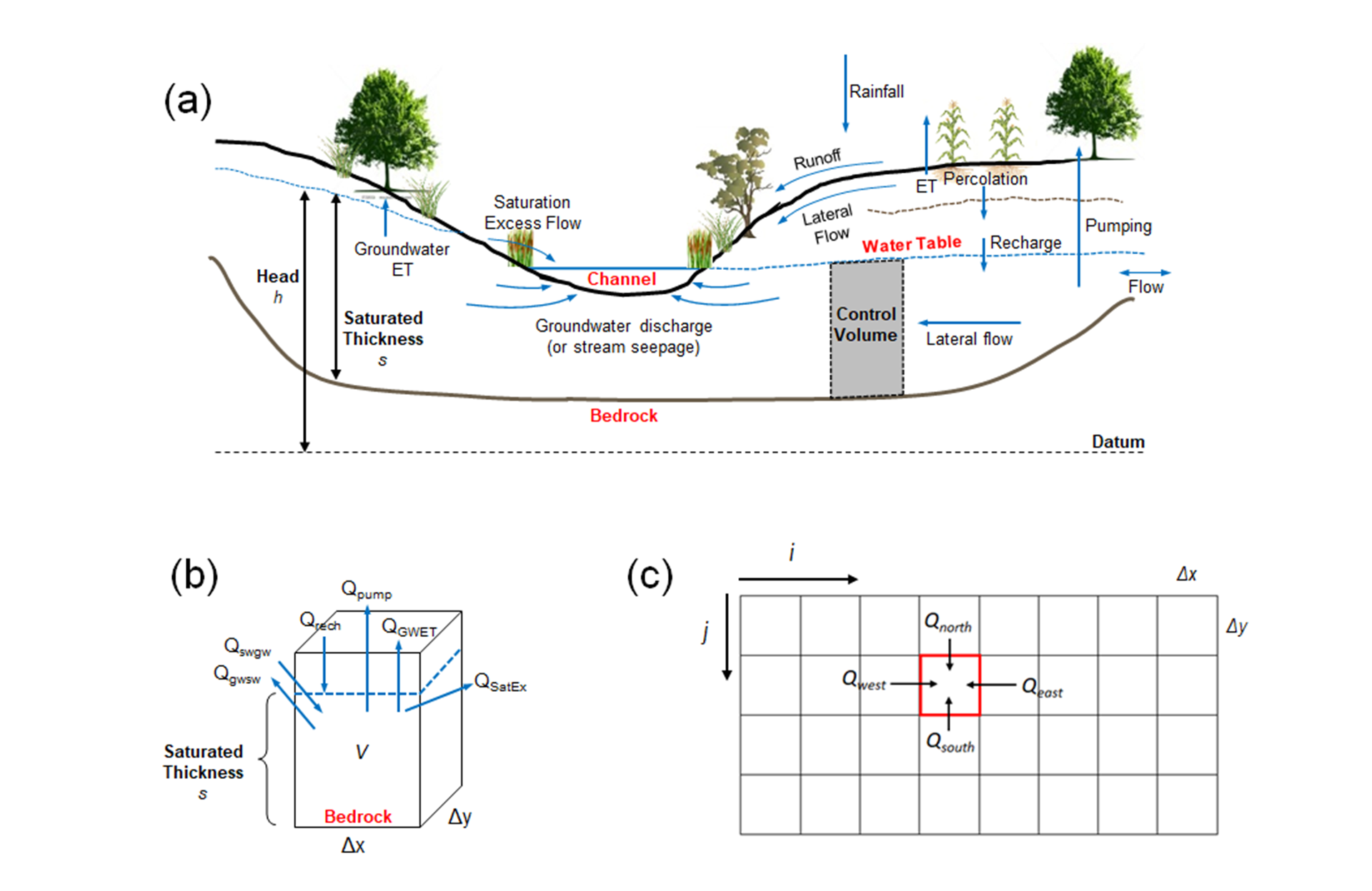
This section describes the method to calculate groundwater volume and groundwater head throughout a heterogeneous unconfined aquifer system within a watershed domain. The hydrologic fluxes in a typical watershed domain are shown in Figure 1a: land surface and soil fluxes include rainfall, runoff, lateral flow, ET, and percolation; groundwater fluxes include lateral flow from each direction (Q_north, Q_south, Q_west, Q_east); flow across the watershed boundary, which is a component of lateral flow; recharge Q_rech; groundwater ET Q_gwet; pumping Q_pump; groundwater discharge to streams Q_gwsw; stream seepage to the aquifer Q_swgw; and saturation excess flow Q_satex, which occurs typically during runoff events related to a rapid rise in the water table and subsequent runoff to streams [29,30,31]. For SWAT+, the land surface and soil hydrologic fluxes are simulated by original SWAT+ routines, whereas the groundwater fluxes are simulated by the new gwflow module. Figure 1a also shows the saturated thickness s of the aquifer (water table to the bedrock) and the head h of groundwater, measured from a datum, typically mean sea level. Within an unconfined flow system, the head h is generally equivalent to water table elevation.

As with all groundwater flow models (e.g., MODFLOW [6], SUTRA [32], CATHY [33], HydroGeoSphere [34]), a control volume approach based on mass conservation is used to establish a water balance equation for each grid cell in the model domain. These equations are then solved for groundwater volume and corresponding groundwater head for each time step of the simulation. Most models use an implicit approach to solve the system of equations, in which head values for all grid cells are updated concurrently (i.e., each head value depends on the head values of surrounding cells at the same time step), and therefore requires linear algebra algorithms or iteration methods. In contrast, the gwflow module uses an explicit approach, in which volume and head values for each grid cell are calculated using information (head values of surrounding grid cells; source and sink fluxes) only from the previous time step. Therefore, each grid cell water balance equation is independent of the equations for surrounding cells and can be solved using a simple loop within a computer program, negating the need for computationally intensive solution algorithms. The explicit solution method was chosen for the gwflow module due to (1) simplicity in coding; and (2) facility in explaining groundwater modeling within the context of watershed systems for watershed modelers. Readers interested in the implicit approach for groundwater modeling are referred to [35].

Although explicit methods have been available for modeling groundwater heads for many years (e.g., [36]), they often are not used due to the requirement of relatively small time steps for solution stability [36]. However, for linking with watershed models that often use daily time steps, the required time step is reasonable, as will be shown in the model application in Section 2.3.

The derivation of the generic aquifer water balance equation is now presented. The aquifer domain within the watershed is discretized into individual control volume cells (i.e., 3D cubes), which in the gwflow module are required to be square on top, e.g., 100 m × 100 m or 200 m × 200, with the thickness of the cell equal to the thickness of the aquifer (ground surface to the bedrock). An example control volume cell and corresponding groundwater fluxes are shown in Figure 1b, with a plan view of the cells shown in Figure 1c. The collection of cells shown in Figure 1c is referred to as a “grid” and covers the area of the watershed. In Figure 1b, the water table is denoted by a dashed blue line, and the saturated thickness s of the cell is the vertical distance from the water table to the bedrock. As the cell is composed of both aquifer material and groundwater, total groundwater volume (m³) in the cell is equal to (Δx·Δy·s·porosity). However, as we are concerned only with groundwater that can be added to/removed from storage, and not with that which is retained due to suction forces between aquifer sediment and groundwater, the groundwater volume V (m³) of concern is:

$$V=\left(\Delta x\cdot \Delta y\cdot s\right)\cdot S_y$$

(1)

where S_y is specific yield (m³ water / m³ of bulk material), i.e., the volume of groundwater released from storage per unit surface area of aquifer per unit decline in groundwater head (i.e., water table) due to gravity.

A volumetric water balance is performed daily for each cell by tracking all groundwater fluxes into/out of the cell:

$$\frac{\Delta V}{\Delta t}={\displaystyle \sum Q_{in}-{\displaystyle \sum Q_{out}}}$$

(2)

where t is time (day), Q_in represents fluxes (m³/day) that add groundwater to the cell, and Q_out (m³/day) represent fluxes that remove groundwater from the cell. Groundwater inputs and outputs can be further categorized into source fluxes, sink fluxes, and lateral fluxes:

$$\frac{\Delta V}{\Delta t}={\displaystyle \sum Q_{source}-{\displaystyle \sum Q_{sink}}}\pm Q_{lateral}$$

(3)

where source fluxes include recharge (Q_rech) and stream seepage (Q_sw→gw) and sink fluxes include groundwater discharge to streams (Q_gw→sw), groundwater ET (Q_gwet), pumping (Q_pump), and saturation excess flow (Q_satex), as shown in Figure 1b. Lateral fluxes are gradient-driven fluxes that flow across the four sides of the cell. The grid in the gwflow module is required to be oriented along north-south and west-east axes, resulting in lateral fluxes in the north, south, west, and east directions (Q_north, Q_south, Q_west, Q_east), as shown in Figure 1c. The “±” sign indicates that flow can either enter the cell from the cell in that direction, or leave the cell towards the cell in that direction. Including these individual flux terms into Equation (2) yields:

$$\frac{\Delta V}{\Delta t}=\left(Q_{rech}+Q_{sw\to gw}\right)-\left(Q_{gwet}+Q_{gw\to sw}+Q_{satex}+Q_{pump}\right)\pm Q_{north}\pm Q_{south}\pm Q_{west}\pm Q_{east}$$

(4)

where lateral fluxes are assumed to add groundwater to the cell. The actual direction of lateral fluxes, i.e., into or out of the cell, depends on groundwater head patterns, as described in Section 2.2.3.

Saturated thickness can be included in the water balance equation of (4) by inserting Equation (1):

$$\frac{\Delta \left[\left(\Delta x\cdot \Delta y\cdot s\right)\cdot S_y\right]}{\Delta t}=\left(Q_{rech}+Q_{sw\to gw}\right)-\left(Q_{gwet}+Q_{gw\to sw}+Q_{satex}+Q_{pump}\right)\pm Q_{north}\pm Q_{south}\pm Q_{west}\pm Q_{east}$$

(5)

Since a change in saturated thickness is equal to a change in groundwater head, h can be substituted for s in Equation (5). Assuming S_y of the aquifer does not change in time yields:

$$\frac{\Delta h}{\Delta t}\left(\Delta x\Delta y{S}_y\right)=\left(Q_{rech}+Q_{sw\to gw}\right)-\left(Q_{gwet}+Q_{gw\to sw}+Q_{satex}+Q_{pump}\right)\pm Q_{north}\pm Q_{south}\pm Q_{west}\pm Q_{east}$$

(6)

Using Equation (3) to simplify notation, the change in head Δh for the grid cell is computed by:

$$\Delta h=\left({\displaystyle \sum Q_{source}-{\displaystyle \sum Q_{sink}}}\pm Q_{lateral}\right)\left(\frac{\Delta t}{S_y\Delta x\Delta y}\right)$$

(7)

which, if assessing a change in head between two points in time n and n+1, h at the next time n+1 can be computed by:

$$h^{n+1}=h^n+\left({\displaystyle \sum Q_{source}-{\displaystyle \sum Q_{sink}}}\pm Q_{lateral}\right)\left(\frac{\Delta t}{S_y\Delta x\Delta y}\right)$$

(8)

Equation (8) is solved for each cell in the grid using cell information (flux terms, h) from the previous time n. Each cell is identified using a row and column index using the i and j notation shown in Figure 1c, leading to:

$$h_{i,j}{}^{n+1}=h_{i,j}{}^n+\left({\displaystyle \sum Q_{sourc{e}_{i,j}}-{\displaystyle \sum Q_{sin{k}_{i,j}}}}\pm Q_{latera{l}_{i,j}}\right)\left(\frac{\Delta t}{S_{y_{i,j}}\Delta x\Delta y}\right)$$

(9)

and now including all flux terms for the gwflow module:

$$h_{i,j}{}^{n+1}=h_{i,j}{}^n+\left[\left(Q_{rech}+Q_{sw\to gw}\right)-\left(Q_{gwet}+Q_{gw\to sw}+Q_{satex}+Q_{pump}\right)\pm Q_{north}\pm Q_{south}\pm Q_{west}\pm Q_{east}\right]\left(\frac{\Delta t}{S_{y_{i,j}}\Delta x\Delta y}\right)$$

(10)

As the computation of h for each cell depends only on information from the previous time n, this solution strategy is an explicit numerical method. Inside the SWAT+ code (see Section 2.2.4 for an explanation of the code structure), the gwflow subroutine loops over the grid cells in the watershed domain, solving for head in each cell using Equation (10). As the head value hⁿ must be known to solve for the head value at the next time step hⁿ⁺¹, the model user must specify the initial head value for each grid cell so that the head values can be calculated on the first day of the SWAT+ simulation. The calculation of each source and sink flux is described in Section 2.2.3. The requirement for solution stability for this explicit approach has been reported [36] as:

$$\frac{\Delta t\cdot K\cdot s}{\Delta x\cdot \Delta y\cdot S_y}\le \frac{1}{4}$$

(11)

Note that Equation (11) does not account for source and sink flux terms. Therefore, the largest Δt that can be used without causing solution instabilities should be found by trial and error when running the model.

2.2.3. Calculating Groundwater Stress Volumetric Fluxes

This section provides details for calculating the individual flux terms in Equation (10) within the context of the SWAT+ modeling code.

Soil Recharge

Recharge to the water table is assumed equivalent to the water percolating from the bottom of the soil profile in each HRU of the SWAT+ model. Similar to SWAT-MODFLOW [10], HRU soil percolation is mapped to grid cell recharge using intersected areas of the HRUs and grid cells. During each daily time step, the depth of recharge from an HRU is multiplied by the area of the HRU to provide a volumetric flow rate in m³/day. This volume is then distributed to grid cells that overlap the HRU, multiplying the volume by the fraction of the HRU that overlaps the grid cell. These fractions are calculated during model construction by intersecting the HRU shapefile and the grid cell shapefile within a GIS, and then placed in an input file gwflow.hrucell.

Lateral Flow

The lateral rate of groundwater flow across the north, south, west, and east sides of each grid cell (see Figure 1c) is calculated using Darcy’s Law:

$$Q=A\cdot K\cdot \frac{\Delta h}{\Delta x}$$

(12)

where A is the cross-sectional area of groundwater flow (m²), K is the hydraulic conductivity of the aquifer material (m/day), and Δh/Δx is the hydraulic gradient, with groundwater flowing from areas of high head to areas of low head. Using the i and j notation from Figure 1c, lateral flux across the west side of a cell (i,j) is written as:

$$Q_{west}=\left(\frac{\Delta x}{\frac{\Delta x/2}{K_{i-1,j}}+\frac{\Delta x/2}{K_{i,j}}}\right)\left[\left(\frac{s_{i-1,j}+s_{i,j}}{2}\right)\Delta y\right]\left(\frac{h_{i-1,j}-h_{i,j}}{\Delta x}\right)$$

(13)

where the first term is the harmonic mean K value of the cell (i,j) and the cell to the west (i−1,j), often used to simulate flow perpendicular to aquifer units; the second term uses the average saturated thickness s (head h–bedrock elevation) from the two cells to estimate A, and the third term uses the h values from the two cells to compute the hydraulic gradient. The third term is written so that higher head in the cell to the west results in a positive gradient, indicating an input of groundwater into the cell (i,j); conversely, lower head in the cell to the west results in a negative gradient, indicating removal of groundwater from the cell (i,j). Similar equations are written for the other three sides:

$$\begin{array}{l}{Q}_{east}=\left(\frac{\Delta x}{\frac{\Delta x/2}{K_{i+1,j}}+\frac{\Delta x/2}{K_{i,j}}}\right)\left[\left(\frac{s_{i+1,j}+s_{i,j}}{2}\right)\Delta y\right]\left(\frac{h_{i+1,j}-h_{i,j}}{\Delta x}\right)\\ Q_{north}=\left(\frac{\Delta x}{\frac{\Delta x/2}{K_{i,j-1}}+\frac{\Delta x/2}{K_{i,j}}}\right)\left[\left(\frac{s_{i,j-1}+s_{i,j}}{2}\right)\Delta x\right]\left(\frac{h_{i,j-1}-h_{i,j}}{\Delta y}\right)\\ Q_{south}=\left(\frac{\Delta x}{\frac{\Delta x/2}{K_{i,j+1}}+\frac{\Delta x/2}{K_{i,j}}}\right)\left[\left(\frac{s_{i,j+1}+s_{i,j}}{2}\right)\Delta x\right]\left(\frac{h_{i,j+1}-h_{i,j}}{\Delta y}\right)\end{array}$$

(14)

Note that for homogeneous aquifer systems, the harmonic mean is simplified to the arithmetic mean of hydraulic conductivity.

Groundwater ET

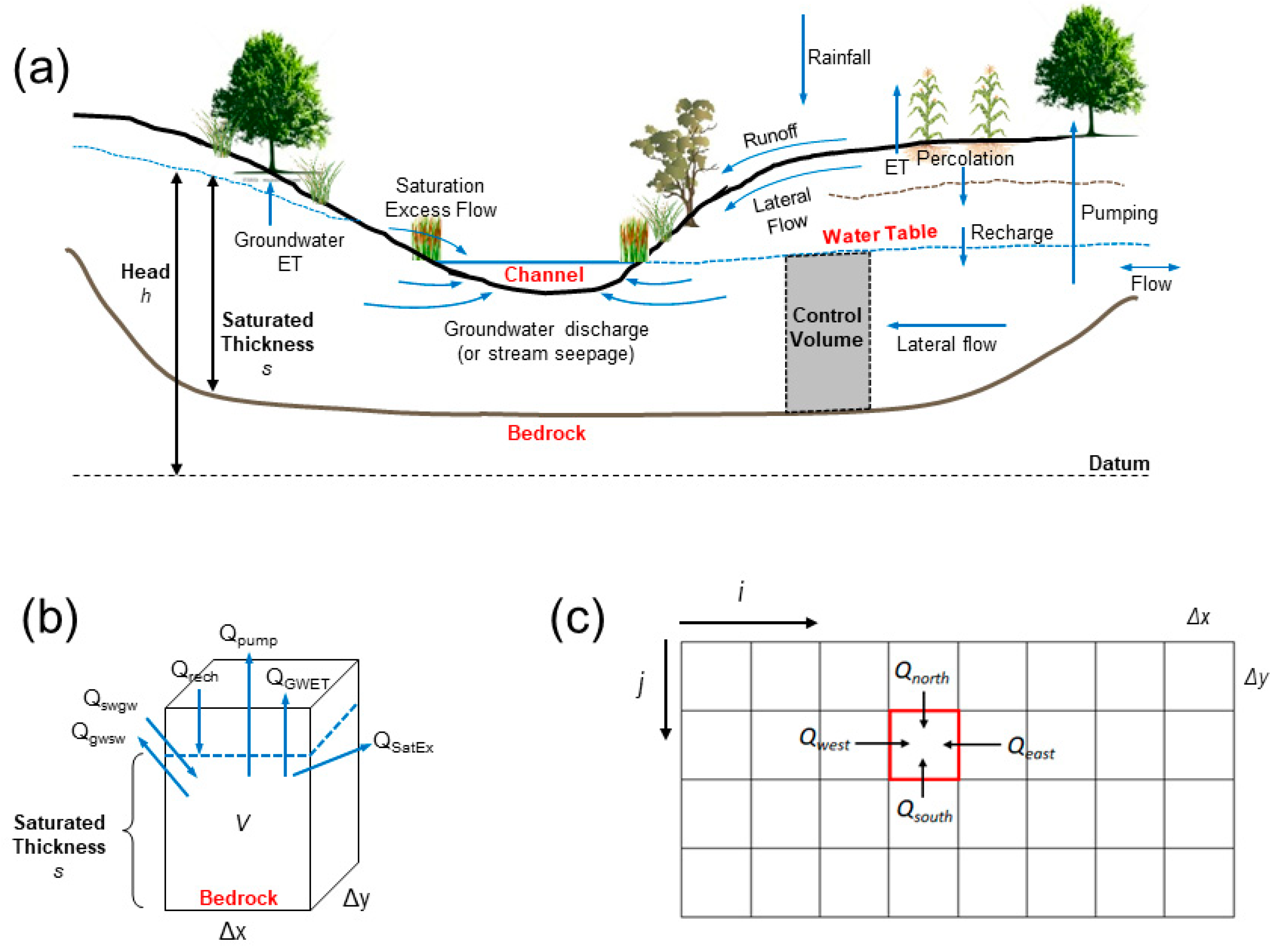
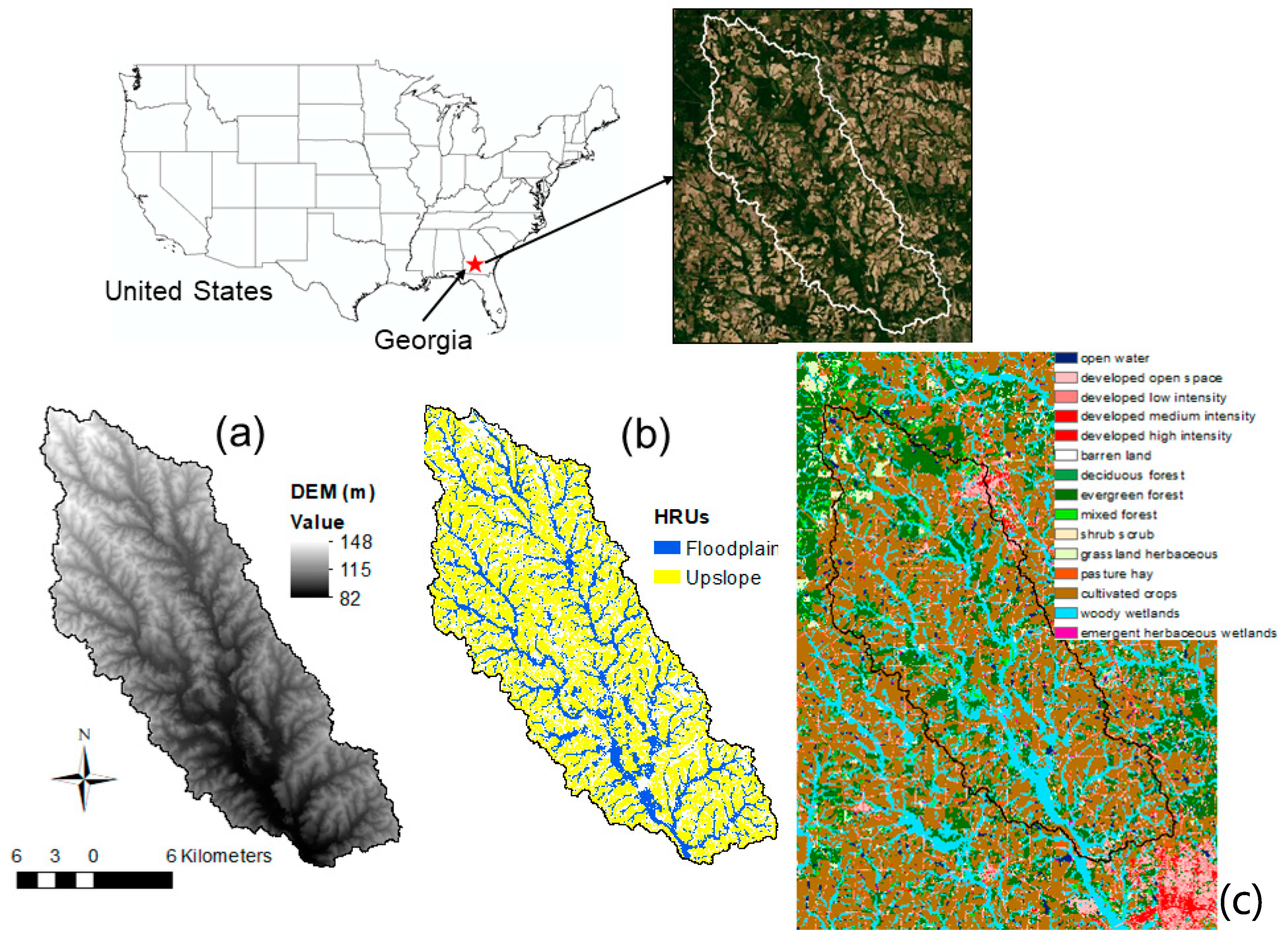
ET from the saturated zone is simulated only if the water table in a cell is above a specified elevation z_bot (m), calculated by subtracting a specified ET extinction depth EXDP (m) (i.e., the depth below which ET cannot occur) from the ground surface z_surf (Figure 2a). The maximum depth of ET that can be removed from the saturated zone is equal to the unsatisfied ET ET_remain (mm), set equal to the difference between the potential ET (mm) and the actual ET (mm) simulated for each HRU for the day. The connection between HRUs and grid cells for mapping unsatisfied ET is the same as for mapping soil percolation to recharge. The depth of groundwater ET_GW (mm) removed from the cell is calculated using the linear relationship from MODFLOW’s EVT package [6]:

$$\begin{array}{l}{h}_{i,j}<z_{bot}\to E{T}_{GW}=0\\ h_{i,j}>z_{bot}\to E{T}_{GW}=E{T}_{remain}\cdot \left(\frac{h_{i,j}-z_{bot}}{z_{surf}-z_{bot}}\right)\end{array}$$

(15)

The depth of ET_GW is multiplied by the horizontal spatial area of the HRU to provide a volumetric flow rate in m³/day, and then divided amongst the cells connected to the HRU, resulting in a Q_gwet value for each cell. This groundwater volume is removed from the cell (see Figure 1b). Figure 2a shows the scenario of Equation (15) within the context of the variables. For the row crop (corn as an example), the condition on the left results in no groundwater ET, whereas the condition on the right would result in ET_GW equal to approximately half of ET_remain. For the tree, the condition would result in ET_GW equal to more than half of ET_remain. Groundwater ET can be significant for areas with high water tables and deep-reaching vegetation roots, e.g., in riparian areas of streams [37,38].

Discharge to Streams and Stream Seepage to the Aquifer

For grid cells that contain streams, Darcy’s Law is used to estimate flow rates between the aquifer and the stream. The direction of flow depends on the relationship between the groundwater head h and the stream stage h_stream. Figure 2b shows the scenario of h > h_stream, resulting in groundwater flow from the aquifer to the stream channel through the streambed with thickness d_bed (m). Flow occurs along the entire length L (m) of the stream within the cell and along the entire bottom width W (m) of the channel. Q_GW→SW (m³/day) for this scenario is estimated by:

$$Q_{GW\to SW}=K_{bed}\left(WL\right)\left(\frac{h-h_{stream}}{d_{bed}}\right)$$

(16)

where K_bed (m/day) is the hydraulic conductivity of the streambed material and (WL) (m²) is the cross-section area of flow. If groundwater head h < h_stream, then stream water recharges the aquifer and Q_SW→GW is calculated. If h is greater than the streambed elevation z_bed, the gradient uses the head difference between h_stream and h; if h is lower than z_bed, the gradient uses the channel depth. These scenarios are summarized in the following set of equations, similar to those in MODFLOW’s River package:

$$\begin{array}{ll}h>h_{stream}& \{\begin{array}{l}{Q}_{GW\to SW}=K_{bed}\left(WL\right)\left(\frac{h-h_{stream}}{d_{bed}}\right)\\ Q_{SW\to GW}=0\end{array}\\ z_{bed}<h<h_{stream}& \{\begin{array}{l}{Q}_{GW\to SW}=0\\ Q_{SW\to GW}=K_{bed}\left(WL\right)\left(\frac{h_{stream}-h}{d_{bed}}\right)\end{array}\\ h<z_{bed}& \{\begin{array}{l}{Q}_{GW\to SW}=0\\ Q_{SW\to GW}=K_{bed}\left(WL\right)\left(\frac{h_{stream}-z_{bed}}{d_{bed}}\right)\end{array}\end{array}$$

(17)

Pumping

Pumping rates Q_pump (m³/day) are specified by the model user. These can be specified for any grid cell, for any day of the simulation in the gwflow.aqu input file.

Saturation Excess Flow

Saturation excess flow occurs when groundwater head h rises above the ground surface, typically during rainfall events that rapidly increase the water table. This condition is tested for each cell during each daily time step. If h > ground surface elevation, the volumetric flux (m³/day) of groundwater excess flow is given by:

$$Q_{satex}=\left(h_{i,j}-z_{sur{f}_{i,j}}\right)\left(\Delta x\Delta y\right)S_{y_{i,j}}$$

(18)

The water is removed from the grid cell and added to the closest stream channel on that same day.

2.2.4. SWAT+ Code Structure with the gwflow Module

The structure of the SWAT+ modeling code with the embedded gwflow module is presented in Figure 3. The gwflow module adds only two subroutines to the SWAT+ code: gwflow_read, which reads data for all grid cells from the input file gwflow.aqu, and gwflow_simulate, which performs the computations of groundwater fluxes and changes in groundwater head and groundwater storage. The subroutine hyd_read_connect, which reads connections between all spatial objects in the SWAT+ model, also reads the input file gwflow.con, which contains a list of connections between grid cells and SWAT+ channels to enable groundwater–surface water interactions (see Section 2.2.4). The inputs required in the gwflow.aqu and gwflow.con files will be discussed in Section 2.2.5.

Following the reading of all input data, the time_control subroutine is called, which controls the yearly and daily computation loops. For each daily time step of the simulation, the command subroutine is called, which loops through all objects (HRUs, Routing Units, channels) in the model, including the gwflow grid cells. When the gwflow_simulate subroutine is called, all groundwater fluxes are calculated, whereupon the change in groundwater storage and groundwater head is calculated for each grid cell. Equations (see Section 2.2.2 and Section 2.2.3) for each calculation are indicated in Figure 3. Head values, groundwater flux values for each grid cell, and a groundwater balance for the entire watershed model domain are then written to files. The groundwater balance is calculated and output for each day, each year, and then for the entire simulation (average annual).

2.2.5. Required Inputs for the gwflow Module

All data for the gwflow module are contained in three input files: gwflow.con, gwflow.aqu, and gwflow.hrucell (see Figure 3). gwflow.con contains a list of all grid cells connected to stream channels, with the ID number listed for each, so that Q_SW→GW and Q_GW→SW can be calculated for the correct cells. These cells are called “River Cells”.

The file gwflow.aqu contains general information for the module and a list of data values for each grid cell. A complete list of information in this file is shown in

Table 2. Information required in the gwflow.aqu file for the gwflow module. Many of the parameters can be found from national or global datasets, as described in the model application in Section 2.3.

Basic Information	Units
Cell size	m
Number of Rows and Columns in the grid	-
Water table initiation flag (1, 2, 3)	-
Saturation excess flow flag (yes/no)	-
Groundwater ET flag (yes / no)	-
Recharge delay	day
Time step Δt	day
Grid Cell Information
Row Index	-
Column Index	-
Status (active = 1, inactive = 0, boundary = 2)	-
Longitude	degree
Latitude	degree
Ground surface elevation	m
Aquifer thickness	m
Hydraulic conductivity zone	-
Specific yield zone	-
Groundwater ET extinction depth EXDP	m
Output Control
Days for groundwater head output	day
Cells for daily groundwater head output	-
River Cell Information
Depth of streambed below DEM value	m
Row Index	-
Column Index	-
Channel ID	-
Stream length in cell	m
Streambed elevation zbed	m
Streambed hydraulic conductivity zone Kbed	-
Streambed thickness zone dbed	-

. Basic information includes the number of rows and columns in the grid, the cell size (m), flags for water table initiation (at the beginning of the simulation) and the inclusion of saturation excess flow and groundwater ET, a recharge delay term (to transfer recharge from the bottom of the soil profile to the water table), and the time step. The water table can be initiated by (1) ground surface minus a specified depth for each grid cell, (2) a fraction of the distance between the ground surface and the bedrock, or (3) a value specified for each cell. For K and S_y, the grid cells are divided into zones, with K and S_y specified for each zone. This facilitates calibration by changing only values for each zone rather than values for each grid cell. Groundwater head h for each cell can be output for any day of the simulation. Certain cells can also be designated as “observation cells”, with h values for these cells output for each day of the simulation, resulting in time series that can be compared to data from groundwater monitoring wells. Many of these data can be obtained from national or global datasets. Sources for these data will be discussed in Section 2.3.

2.3. Application to the Little River Experimental Watershed, Georgia

2.3.1. Overview of Study Region

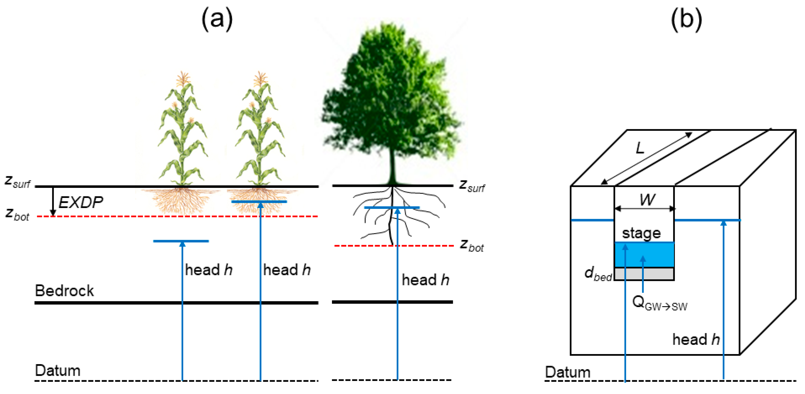
The SWAT+ model using the new gwflow module is applied in this study to the 327 km² Little River Experimental Watershed (LREW), located within the Upper Suwannee River Basin in south-central Georgia (Figure 4). This watershed is ideal for testing the gwflow module due to the strong connection between the shallow unconfined aquifer and the many streams that make up the river system [31]. In addition, there are a number of streamflow gages and groundwater monitoring wells located throughout the watershed for model testing.

The climate of the region is humid subtropical, with hot and humid summers and mild winters. Summers are characterized by high-intensity thunderstorms, leading to sharp increases in streamflow. The average annual rainfall is approximately 1200 mm, and the annual mean temperature is 19 °C. The average annual ET has been estimated to be approximately 70% of annual precipitation [37]. The watershed elevation ranges between 82 m and 148 m, with broad floodplains (Figure 4a). Land use (Figure 4c) consists of forest (50%), primarily pine trees in upland areas and hardwoods and evergreens in riparian areas; agriculture, primary cotton and peanut row-crops (41%); urban areas (7%), and open water (2%). Soils are loamy sands and sandy loams [39], which are underlain by the relatively impermeable Hawthorne formation which limits groundwater flow to deeper geologic layers [40]. The presence of the Hawthorne formation, referred to as the bedrock through the remainder of this paper, leads to significant lateral groundwater flow and associated groundwater discharge to streams [31,37,41]. Saturation excess flow conditions occur within the riparian areas [42]. The thickness of the alluvial aquifer is presented in Section 2.3.3.

Many variations and applications of the SWAT and SWAT+ models have been applied to the LREW, including for model evaluation, calibration, and parameter sensitivity [43,44,45,46], analyzing the effect of conservation practices on water quality [47], landscape routing [48] and connectivity between upland areas and floodplains [28]. Indeed, the SWAT+ model was first published and introduced using an application to this watershed [2]. These applications, however, treated groundwater flow and groundwater–surface water interactions simplistically, based on steady flow assumptions and unconnected aquifer regions. The inclusion of the gwflow module is expected to simulate more realistic groundwater hydrologic fluxes, which can lead to improved assessments of riparian-stream hydrology and conservation practices within the study region.

2.3.2. SWAT+ Model Construction

The base SWAT+ model was constructed using QSWAT+, a QGIS interface for SWAT+ (https://swat.tamu.edu/software/plus/). The interface guides the user through loading datasets (DEM, land use and crop data, soil type, and climate station data) and creating hydrologic response units (HRUs), routing units, and channels. The resolution and source for each data set are shown in

Table 3. Datasets and corresponding sources for the construction of the Little River Watershed SWAT+ model.

Data	Resolution	Source
Topo-graphy	30 m	U.S. Geological Survey, National Elevation Data
		Accessed: 15 October 2019, https://viewer.nationalmap.gov
Land use	30 m	U.S. Geological Survey, National Land Cover Data (2016)
		Accessed: 15 October 2019, https://www.mrlc.gov/data
Crop Data	30 m	U.S. Dept. of Agriculture, CropScape
		Accessed: 15 October 2019, https://nassgeodata.gmu.edu/CropScape/
Soil	30 m	USDA-NRCS, Soil Survey Geographic (SSURGO)
		Accessed: 15 October 2019, -https://datagateway.nrcs.usda.gov/
Climate	Multiple stations	Precipitation: daily watershed weighted average [51].
		Other climate variables: SWAT+ global database.
Aquifer thickness (cm)	250 m	[52]
		Accessed: 10 December 2019, https://soilgrids.org/
Hydraulic conduct. (m/day)	Vector Polygons	[53]
		Accessed: 10 December 2019, https://dataverse.scholarsportal.info/dataset.xhtml?persistentId=doi:10.5683/SP2/TTJNIU

. The interface then uses the SWAT+ Editor to write all necessary input files to run the SWAT+ modeling code. In this study, SWAT+ version 59.3 is used. The process resulted in 10796 HRUs and 343 channels. Figure 4b shows the HRUs divided into upland areas (yellow) and floodplains areas (blue). Channel delineation is shown in Section 2.3.3.

Before including the gwflow module, an initial calibration was performed for SWAT+ to provide hydrologic fluxes (surface runoff, lateral flow, groundwater discharge, ET) that are similar to those observed from field data assessment. This calibration was performed manually as well as using IPEAT+ (Integrated Parameter Estimation and Uncertainty Analysis Tool Plus) [49], an automated calibration tool developed for SWAT+, based on the Dynamically Dimensioned Search (DDS) algorithm [50], using the streamflow at the watershed outlet as testing data.

2.3.3. Preparing the gwflow Module

Preparing the gwflow module for SWAT+ consists of populating the gwflow.aqu, gwflow.hrucell, and gwflow.con files. The following list provides details regarding the preparation of all required data for the gwflow.aqu file (see Table 2). All data can be prepared in a GIS (e.g., ArcMap, QGIS).

• Cell size: defined by the user, typically between 100 and 500 m on a side based on previous applications of coupled surface water–groundwater models such as SWAT-MODFLOW (e.g., [14,16]). In the current edition of the code, all cells must be the same size.
• Number of rows and columns: based on the extent of the watershed and the specified cell size.
• Time step Δt: The maximum time step is 1 day, since the gwflow module is called each day within the SWAT+ code (see Figure 3). The minimum required time step must be found using a trial and error approach. We recommend starting with 1 day, checking results in the daily groundwater balance file to verify that the percent error in groundwater balance is equal to 0.
• Status (active, inactive, boundary): as the grid is rectangular in shape, many cells will be located outside the watershed boundary; these cells are “inactive” and assigned status = 0. All cells within the watershed boundary are “active” and assigned status = 1, except for cells that lie along the boundary and are designated as “boundary” cells and assigned status = 2. Boundary cells are simulated as constant-head cells, i.e., the groundwater head assigned to these cells at the beginning of the simulation remains constant throughout the simulation period.
• Groundwater surface elevation: obtained from the DEM of the watershed.
• Aquifer thickness (m): obtained from [52], who provide a global map of unconsolidated sediment thickness (cm) from the ground surface to bedrock (see Table 2). This dataset is particularly useful for watersheds with limited borehole and drilling information. These values must be converted to meters for the gwflow module.
• Hydraulic conductivity K (m/day): obtained from [53], who provide a global map of permeability (see Table 2). Permeability must be converted to K in m/day.
• Specific Yield S_y: specific yield values (typically 0.10 to 0.30 for alluvial aquifer sediments) are estimated based on the values of K, i.e., if values of K coincide with a certain material (e.g., sand, silt), specific yield values for this material type are also used.
• River Cell information: River Cells are identified by intersecting the grid cells with the SWAT+ channels; streambed elevation is calculated using the elevation of the cell (from the DEM) minus a specific depth (Depth of streambed below DEM value), recognizing that the actual streambed elevation is likely much lower than the average elevation of a DEM raster cell. Initial K_bed and d_bed values can be based on literature.

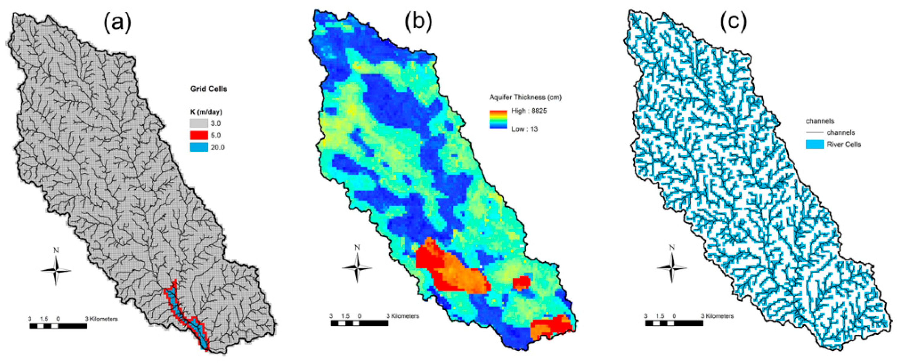
This study uses 200 m grid cells for the gwflow module, resulting in 8647 active cells. The grid and associated K values are shown in Figure 5a. These K values (3 m/day, 5 m/day, 20 m/day) are the final values based on manual calibration (see Section 2.3.4), and were increased from the values (0.001 m/dy, 0.086 m/day, 1.369 m/day) provided by the global data set. Corresponding S_y values are 0.10, 0.15, and 0.11. As shown in Figure 5a, there are only 3 zones of aquifer materials. K_bed and d_bed were set to 0.001 m/day and 2 m, respectively, for all River Cells. The aquifer thickness (cm) (Figure 5b) ranged from 0.13 m to 88.2 m. The identified River Cells are shown in Figure 5c.

2.3.4. Overall Simulation

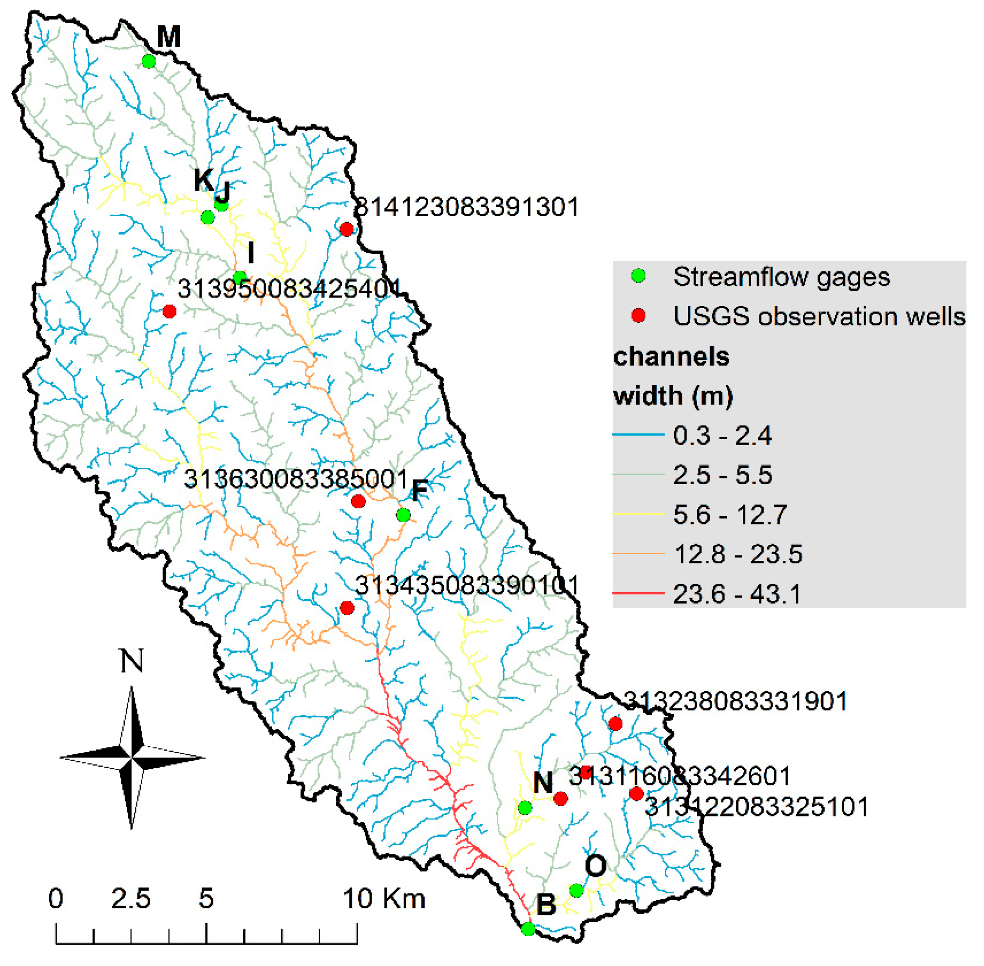
The simulation is run for the 1980–2013 period, with the first two years used as a warm-up (i.e., the results from 1980 and 1981 are not compared to observed watershed data). Based on initial simulations, a time step Δt of 0.25 days was required for the stability of the groundwater balance equation (Equation (10)). The run time of the model is only 20% higher than the original SWAT+ simulation due to the additional equations added to SWAT+ by the gwflow module. Simulated daily streamflow was compared to average daily streamflow at 8 gage sites, provided by the USDA-ARS (Agricultural Research Service) Southeast Watershed Research Laboratory, and simulated daily groundwater head was compared to periodic groundwater levels measured at 8 monitoring wells, provided by the U.S. Geological Survey (USGS) (https://maps.waterdata.usgs.gov/mapper/index.html, accessed 15 February 2020). Figure 6 shows the location of the streamflow gages (green dots) and monitoring wells (red dots).

Only manual calibration was performed in this study, to provide reasonable matches between simulated and observed streamflow and groundwater head. The Nash–Sutcliffe Efficiency (NSE) coefficient is used to quantify the performance of the model regarding streamflow simulation. For aquifer properties K and S_y, values were changed only according to the three identified zones (see Figure 5a) to remain consistent with the global data set, and therefore point-by-point calibration was not pursued to yield optimal matches between simulated and observed groundwater head at the 8 monitoring wells. Automated calibration could be performed to yield optimal matches for both groundwater head and streamflow. However, the intent of this paper is to present the gwflow module and its basic workings rather than prepare a model for scenario analysis.

3. Results and Discussion

3.1. Water Balance

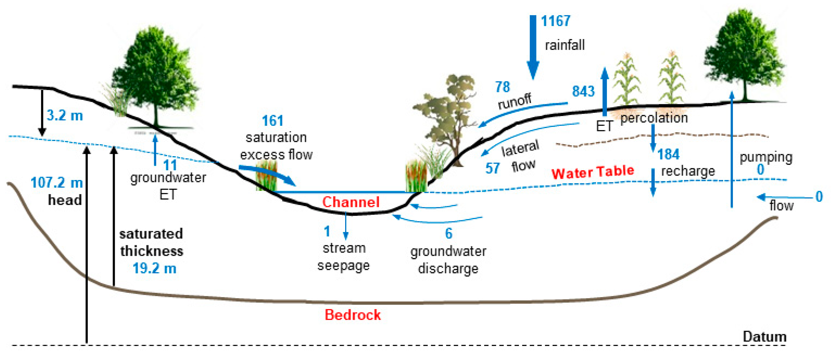
The overall water balance of the SWAT+ simulation is shown in Figure 7 using average annual flux values in mm (depth over the entire watershed). For simulations using the original SWAT+ code, fluxes would be limited to surface runoff (78 mm), lateral flow (57 mm), ET (843 mm), percolation and recharge (184 mm), and groundwater discharge. With the inclusion of the gwflow module, additional fluxes include boundary flow (0 mm), groundwater discharge (6 mm), stream seepage (1 mm), groundwater ET (11 mm), and saturation excess flow (161 mm), with state variables groundwater head (average of 107.2 m for the watershed) and saturated thickness (average of 19.2 m). Surface runoff (78 mm) and lateral flow (57 mm) account for 12% of annual precipitation, whereas groundwater accounts for 14% of annual precipitation. Water yield is 26% of annual precipitation, close to the observed value of 27% [31]. Groundwater entering streams occurs primarily via saturation excess flow (161 mm) rather than groundwater discharge (6 mm).

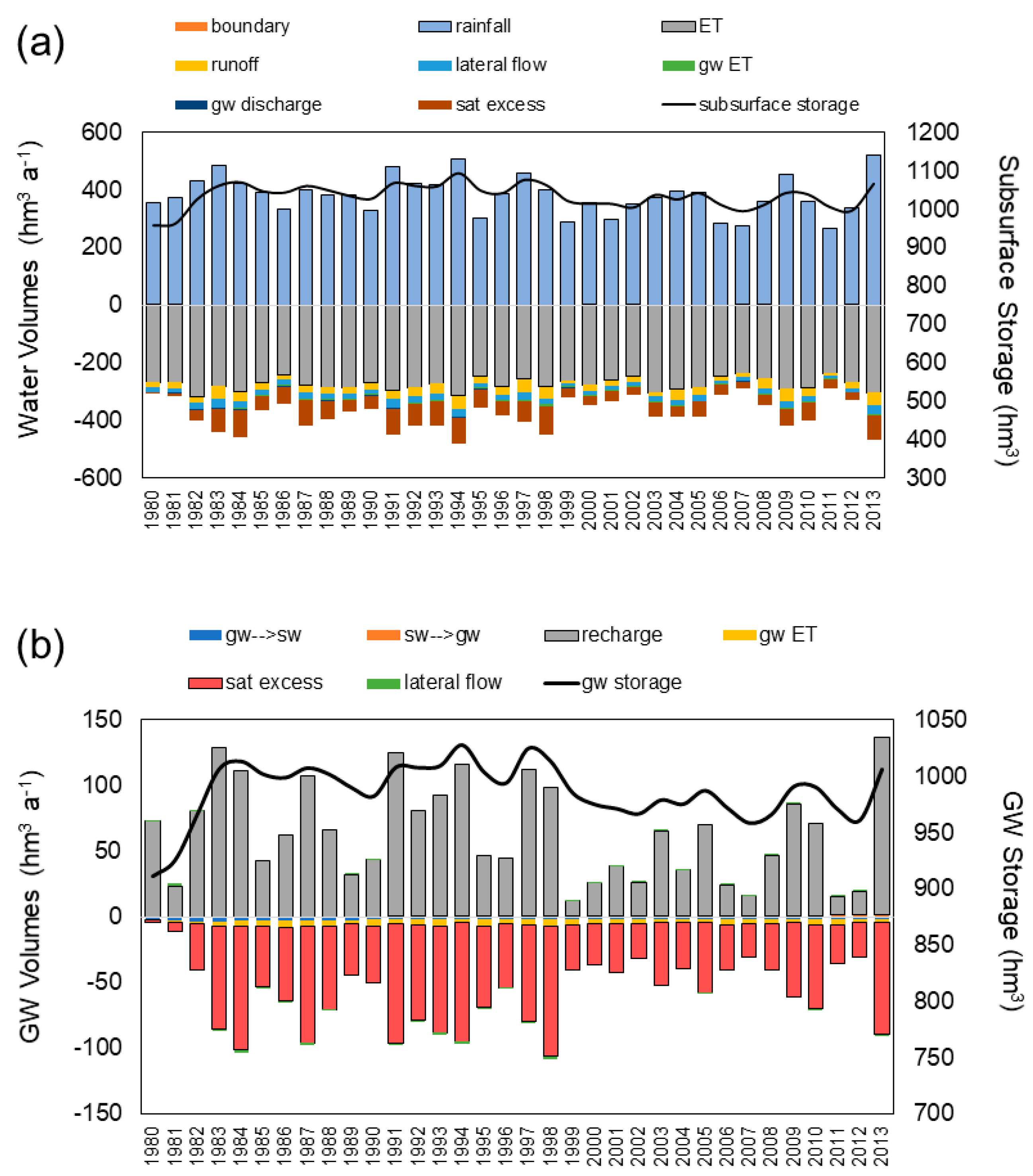
Total water inputs include rainfall (1167 mm), total outputs equal 1155 mm, and the total change in groundwater storage and soil water storage is 15 mm and 1 mm, respectively, resulting in a water balance error of 0.4%. A time series of volumetric amounts (m³ × 10⁶) for all hydrologic fluxes is shown in Figure 8a, with positive values indicating water entering the watershed, and negative values indicating water leaving the watershed. The year-by-year subsurface storage volume (groundwater + soil water) also is shown. A similar time series is shown in Figure 8b for the aquifer system, with positive values indicating water entering the aquifer (sources), and negative values indicating groundwater leaving the aquifer (sinks). The year-by-year groundwater storage volume also is shown. The percent error in the groundwater balance is < 0.00001%.

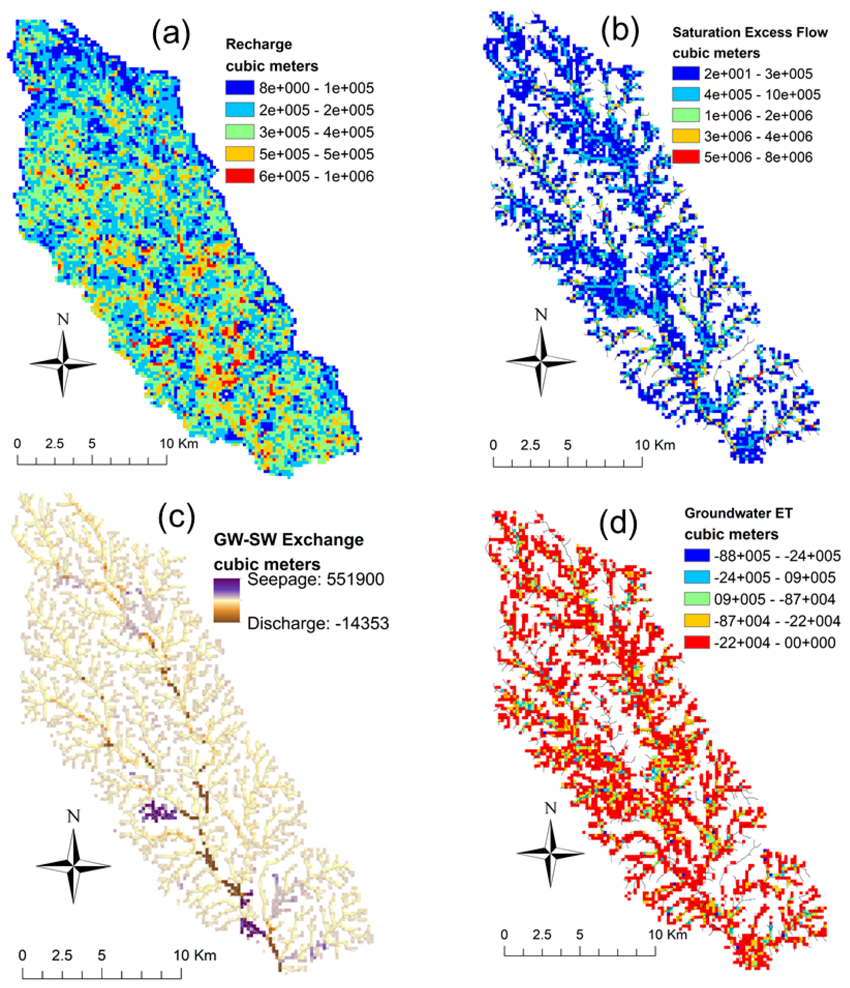
The aquifer system time series (Figure 8b) shows that recharge is largely balanced by saturation excess flow, i.e., recharge events during large storm events produce saturation excess flow near the streams. This is demonstrated further in the maps (Figure 9) of spatial varying volumetric fluxes (m³) over the 1980–2013 simulation period for recharge, saturation excess flow, groundwater–surface water exchange, and groundwater ET. Saturation excess flow occurs primarily in the riparian areas, as does groundwater ET, with the latter due to riparian trees extracting water from the water table [54].

3.2. Streamflow Results

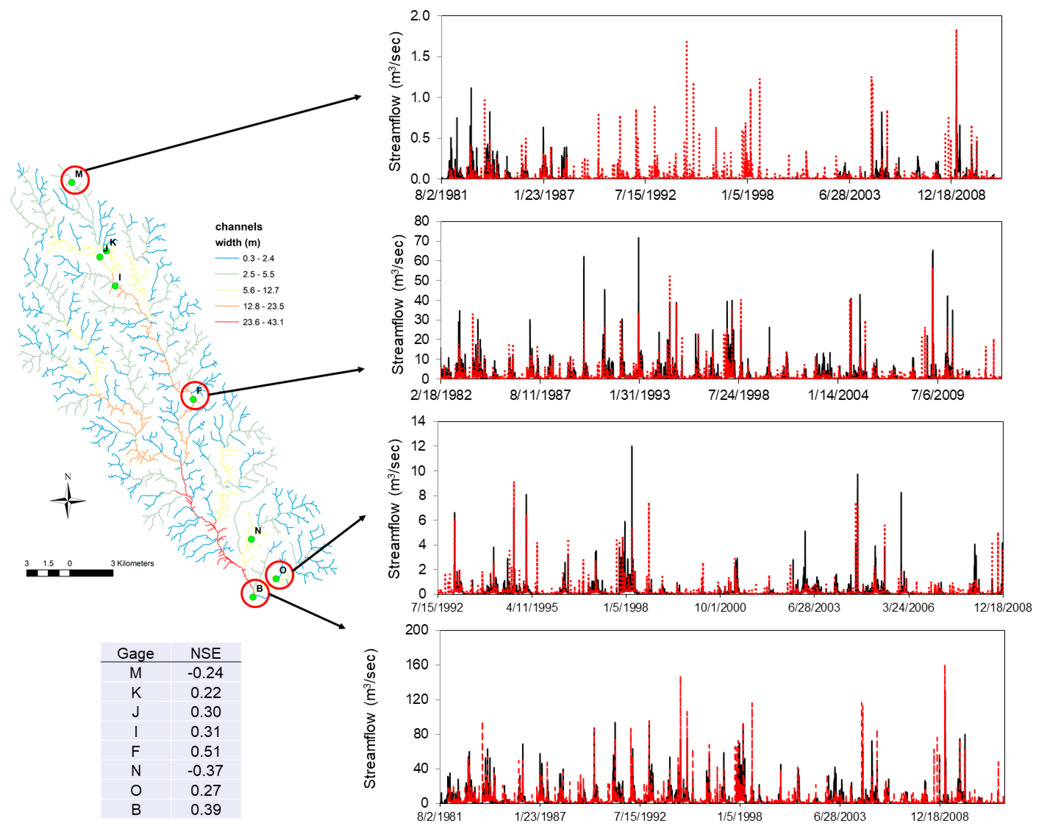
Time series of daily simulated and observed streamflow (m³/sec) are shown in Figure 10 for four of the stream gage sites from the upstream to downstream end of the watershed. The NSE value for each of the eight sites is shown in the inset table. Although several sites show adequate values (J, I, F, B: ≥ 0.30), others show poor matches (K, O: 0.22 and 0.27) and two are below 0 (M, N: −0.24, −0.37). Note that sites K, O, M and N are along small tributaries of the river system with moderate (< 15 m³/s) or low flows (< 5 m³/s). However, visual comparisons (see time series charts for M and O in Figure 10) indicate that the model does track the timing of measured flow. This is encouraging, as these flows are controlled to a large degree by subsurface flows calculated by the gwflow module. Detailed calibration of subbasin parameters for these tributary regions would be necessary if the model is to be used for scenario analysis. As this model application is intended solely for gwflow module demonstration, the results are adequate.

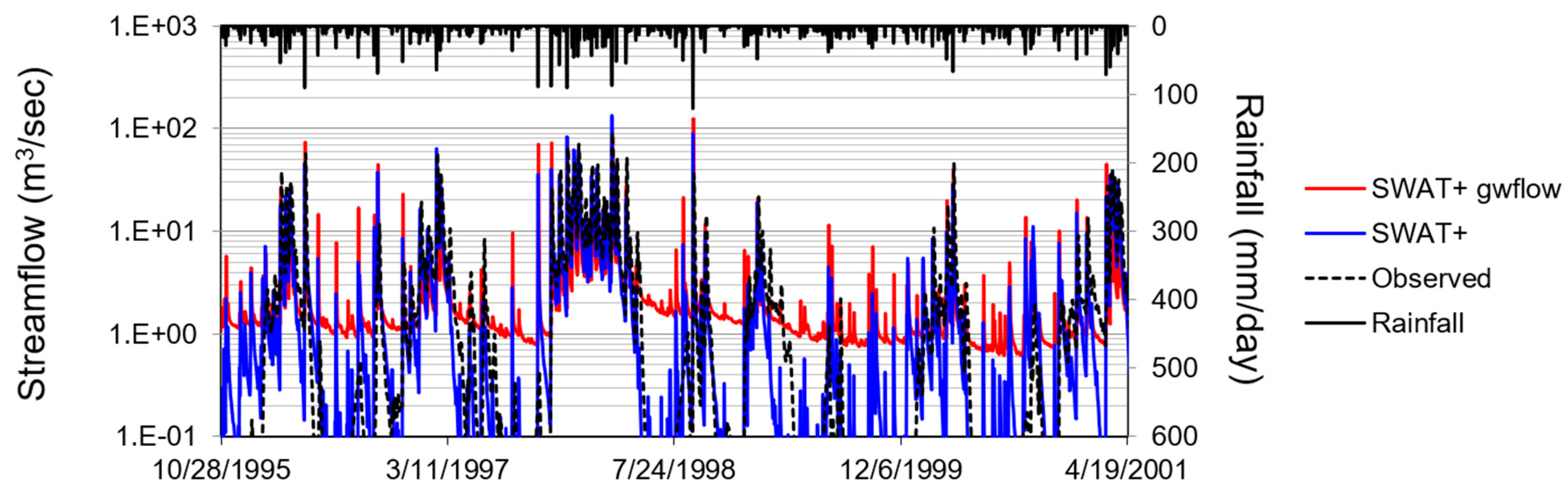
The differences in simulated streamflow between the original SWAT+ model and the SWAT+ model with the gwflow module are shown in Figure 11 for the outlet (site B) for several years of the simulation. As seen by the time series, SWAT+ simulates near-zero flow between rainfall events, consistent with the measured streamflow, whereas SWAT+ with gwflow simulates low flows (1–3 m³/s) during these times. Groundwater discharge in SWAT+ is simulated in the “pulse” form, based on the magnitude of rainfall events and the resulting recharge. Using the gwflow module, however, groundwater can enter the streams at any time based on groundwater gradients, leading to small flows between rainfall events. The results of SWAT+ are more accurate in this instance in this regard, as observed flows also approach zero between rainfall events during certain times of the year. As such, further calibration is required for the gwflow module if these low-flow periods are of importance for the intended use of the model. However, the inclusion of the gwflow module allows groundwater discharge to streams, either via the streambed or via saturation excess flow, to be simulated in a more physically realistic manner for scenario analysis (e.g., climate change, water conservation, nutrient management).

3.3. Groundwater Head Results

Groundwater head (m) at the end of the simulation (end of 2013) for each grid cell is shown in Figure 12. The groundwater head (i.e., water table elevation) mimics the ground surface elevation (see Figure 4a). Groundwater head fluctuations are also shown at the eight monitoring well locations, in comparison with the observed groundwater head values from the USGS data set. The dotted brown line on each time series chart represents the ground surface at that site. Observed rapid groundwater head fluctuations generally are captured by the model. The rapid changes occur due to recharge events and resulting lateral flow and/or saturation excess flow.

The mean absolute error (MAE) of simulated head values that correspond in location and timing to measured head values is 1.7 m. All sites have an MAE of 3.0 m or less. Two locations (313144083335501, 313238083331901) show excellent tracking of the measured head by the model, while others show moderate agreement. For several locations, the model underpredicts head levels, and at two locations (313435083390101, 313630083385001) the model overestimates head levels. The underestimation and overestimation could be due to the misrepresentation of aquifer properties (K, S_y) or underestimation of localized recharge by HRUs. Likely the aquifer properties are not represented correctly for these localized areas. However, as with the streamflow results shown in Section 3.2, in this study aquifer property values are constrained by the zones established by the global permeability map (see Figure 5a). Point-by-point calibration could be performed to provide better matches between the observed and simulated head values; however, the purpose of this paper is to present the gwflow module and to highlight its capabilities. If the model is to be used for scenario analysis, localized aquifer conditions can be better represented using borehole lithology data. Such an approach would also use automated parameter estimation methods and employ ensemble-based uncertainty analysis and sensitivity analysis methods (e.g., [21,22,23]) to explore the effect of parameter values (e.g., hydraulic conductivity: [24,25]) on system-response variables such as water table elevation, groundwater–surface water exchange rates, and streamflow.

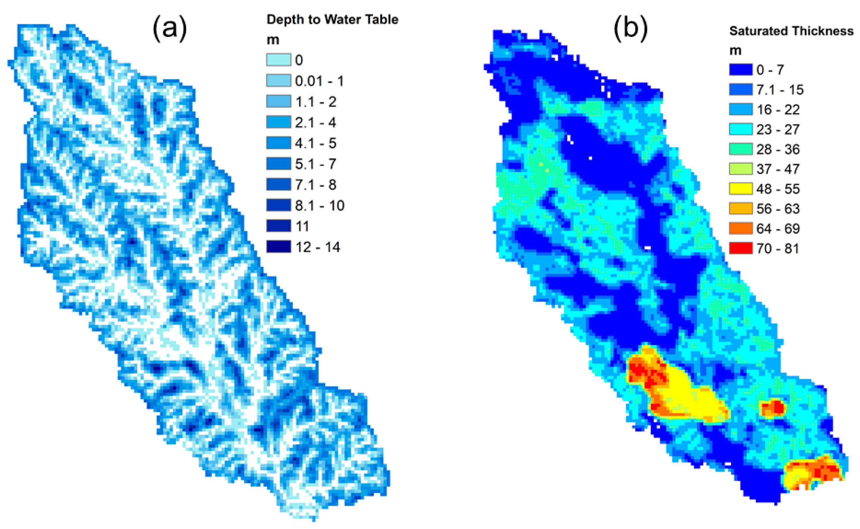
Finally, depth to water table (m) and saturated thickness (m) for each grid cell at the end of the simulation are shown in Figure 13. The map of depth to water table shows depths near 0 or at 0 for much of the riparian and floodplain areas, indicating near-saturated conditions, leading to groundwater ET (see Figure 9d) and saturation excess flow (see Figure 9b). The map of saturated thickness shows spatial patterns similar to the map of aquifer thickness (see Figure 5b). Such maps can assist in determining groundwater storage throughout the aquifer system and the strong interplay between the land surface and subsurface hydrologic processes.

4. Summary and Conclusions

This paper presents a new physically-based spatially-distributed groundwater flow module (gwflow) for the SWAT+ watershed model. The module is embedded in the SWAT+ modeling code as with other hydrologic modules and is intended to replace the current SWAT+ aquifer module [2] for watersheds with strong stream-aquifer connections. The model accounts for recharge from SWAT+ HRUs, lateral flow within the aquifer, ET from shallow groundwater, pumping, groundwater–surface water interactions through the streambed, and saturation excess flow. Daily groundwater head and groundwater storage are solved using an explicit numerical method approach for the groundwater balance equation, with head and flow values for the current day based on head and flow values from the previous day. The module outputs groundwater head and flux rates for each groundwater stress for analysis and mapping.

The modified SWAT+ model is applied to the 327 km² Little River Experimental Watershed in southern Georgia, USA, demonstrating its capabilities of simulating both surface and subsurface hydrological processes. Results from an uncalibrated model are compared against measured streamflow and groundwater levels at eight stream gage sites and eight groundwater monitoring locations, respectively. The model performed adequately regarding visual comparisons of time series and quantitative statistics but can be improved with additional calibration if it is to be used for scenario analysis. For this watershed, groundwater additions to the stream system are governed by saturation excess flow rather than discharge via the streambed, based on continual near-saturation conditions in the riparian areas and measured low baseflow between rainfall events. For this watershed, inclusion of the gwflow module increases SWAT+ model run time by approximately 20%.

The modified SWAT+ modeling code with the gwflow module can be an important tool for modeling hydrological fluxes in watersheds that have a strong connection between the shallow unconfined aquifer and the stream system. Using this code can provide physically realistic groundwater flow gradients, flux values, and interactions with streams, which are important for assessing the effects of conservation practices on hydrology and nutrient transport.

References

- Arnold, J.G.; Srinivasan, R.; Muttiah, R.S.; Williams, J.R. Large area hydrologic modeling and assessment part I: Model development. JAWRA J. Am. Water Resour. Assoc. 1998, 34, 73–89. [Google Scholar] [CrossRef]
- Bieger, K.; Arnold, J.G.; Rathjens, H.; White, M.J.; Bosch, D.D.; Allen, P.M.; Volk, M.; Srinivasan, R. Introduction to SWAT+, A Completely Restructured Version of the Soil and Water Assessment Tool. JAWRA J. Am. Water Resour. Assoc. 2017, 53, 115–130. [Google Scholar] [CrossRef]
- Srivastava, P.; McNair, J.N.; Johnson, T.E. Comparison of process-based and artificial neural network approaches for streamflow modeling in an agricultural watershed. JAWRA J. Am. Water Resour. Assoc. 2006, 42, 545–563. [Google Scholar] [CrossRef]
- Gassman, P.W.; Reyes, M.R.; Green, C.H.; Arnold, J.G. The Soil and Water Assessment Tool: Historical Development, Applications, and Future Research Directions. Trans. ASABE 2007, 50, 1211–1250. [Google Scholar] [CrossRef] [Green Version]
- Deb, P.; Kiem, A.S.; Willgoose, G. A linked surface water-groundwater modelling approach to more realistically simulate rainfall-runoff non-stationarity in semi-arid regions. J. Hydrol. 2019, 575, 273–291. [Google Scholar] [CrossRef]
- Harbaugh, A.W. MODFLOW-2005, The U.S. Geological Survey Modular Ground-Water Model—The Ground-Water Flow Process; USGS Techniques and Methods 2005 6-A16, US Geological Survey; US Department of the Interior: Reston, VA, USA, 2005.
- Galbiati, L.; Bouraoui, F.; Elorza, F.J.; Bidoglio, G. Modeling diffuse pollution loading into a Mediterranean lagoon: Development and application of an integrated surface–subsurface model tool. Ecol. Model. 2006, 193, 4–18. [Google Scholar] [CrossRef]
- Kim, N.W.; Chung, I.-M.; Won, Y.S.; Arnold, J.G. Development and application of the integrated SWAT-MODFLOW model. J. Hydrol. 2008, 356, 1–16. [Google Scholar] [CrossRef]
- Guzman, J.A.; Moriasi, D.N.; Gowda, P.H.; Steiner, J.L.; Starks, P.J.; Arnold, J.G.; Srinivasan, R. A model integration framework for linking SWAT and MODFLOW. Environ. Model. Softw. 2015, 73, 103–116. [Google Scholar] [CrossRef]
- Bailey, R.T.; Wible, T.C.; Arabi, M.; Records, R.M.; Ditty, J. Assessing regional-scale spatio-temporal patterns of groundwater-surface water interactions using a coupled SWAT-MODFLOW model. Hydrol. Process. 2016, 30, 4420–4433. [Google Scholar] [CrossRef]
- Aliyari, F.; Bailey, R.T.; Tasdighi, A.; Dozier, A.; Arabi, M.; Zeiler, K. Coupled SWAT-MODFLOW model for large-scale mixed agro-urban river basins. Environ. Model. Softw. 2019, 115, 200–210. [Google Scholar] [CrossRef]
- Chunn, D.; Faramarzi, M.; Smerdon, B.; Alessi, D.S. Application of an Integrated SWAT-MODFLOW Model to Evaluate Potential Impacts of Climate Change and Water Withdrawals on Groundwater–Surface Water Interactions in West-Central Alberta. Water 2019, 11, 110. [Google Scholar] [CrossRef] [Green Version]
- Gao, F.; Feng, G.; Han, M.; Dash, P.; Jenkins, J.; Liu, C. Assessment of Surface Water Resources in the Big Sunflower River Watershed Using Coupled SWAT-MODFLOW Model. Water 2019, 11, 528. [Google Scholar] [CrossRef] [Green Version]
- Molina-Navarro, E.; Bailey, R.T.; Andersen, H.E.; Thodsen, H.; Nielsen, A.; Park, S.; Jensen, J.S.; Jensen, J.B.; Trolle, D. Comparison of abstraction scenarios simulated by SWAT and SWAT-MODFLOW. Hydrol. Sci. J. 2019, 64, 434–454. [Google Scholar] [CrossRef]
- Semiromi, M.T.; Koch, M. Analysis of spatio-temporal variability of surface-groundwater interactions in the Gharehsoo river basin, Iran, using a coupled SWAT-MODFLOW model. Environ. Earth Sci. 2019, 78, 201. [Google Scholar] [CrossRef]
- Wei, X.; Bailey, R.T. Assessment of System Responses in Intensively Irrigated Stream–Aquifer Systems Using SWAT-MODFLOW. Water 2019, 11, 1576. [Google Scholar] [CrossRef] [Green Version]
- Bailey, R.T.; Park, S.; Bieger, K.; Arnold, J.G.; Allen, P.M. Enhancing SWAT+ simulation of groundwater flow and groundwater-surface water interactions using MODFLOW routines. Environ. Model. Softw. 2020, 126, 104660. [Google Scholar] [CrossRef]
- Raymond, H.A.; Bondoc, M.; McGinnis, J.; Metropulos, K.; Heider, P.; Reed, A.; Saines, S. Using Analytic Element Models to Delineate Drinking Water Source Protection Areas. Ground Water 2006, 44, 16–23. [Google Scholar] [CrossRef]
- Brown, K.; Trott, S. Groundwater Flow Models in Open Pit Mining: Can We Do Better? Mine Water Environ. 2014, 33, 187–190. [Google Scholar] [CrossRef]
- Jones, D.; Jones, N.L.; Greer, J.; Nelson, J. A cloud-based MODFLOW service for aquifer management decision support. Comput. Geosci. 2015, 78, 81–87. [Google Scholar] [CrossRef]
- Yang, J.; Reichert, P.; Abbaspour, K.C.; Xia, J.; Yang, H. Comparing uncertainty analysis techniques for a SWAT application to the Chaohe Basin in China. J. Hydrol. 2008, 358, 1–23. [Google Scholar] [CrossRef]
- Strauch, M.; Bernhofer, C.; Koide, S.; Volk, M.; Lorz, C.; Makeschin, F. Using precipitation data ensemble for uncertainty analysis in SWAT streamflow simulation. J. Hydrol. 2012, 414, 413–424. [Google Scholar] [CrossRef]
- Muleta, M.K.; Nicklow, J.W. Sensitivity and uncertainty analysis coupled with automatic calibration for a distributed watershed model. J. Hydrol. 2005, 306, 127–145. [Google Scholar] [CrossRef] [Green Version]
- Colombo, L.; Alberti, L.; Mazzon, P.; Formentin, G. Transient Flow and Transport Modelling of an Historical CHC Source in North-West Milano. Water 2019, 11, 1745. [Google Scholar] [CrossRef] [Green Version]
- Moeck, C.; Molson, J.; Schirmer, M. Pathline Density Distributions in a Null-Space Monte Carlo Approach to Assess Groundwater Pathways. Ground Water 2020, 58, 189–207. [Google Scholar] [CrossRef] [PubMed]
- Park, S.; Nielsen, A.; Bailey, R.T.; Trolle, D.; Bieger, K. A QGIS-based graphical user interface for application and evaluation of SWAT-MODFLOW models. Environ. Model. Softw. 2019, 111, 493–497. [Google Scholar] [CrossRef]
- Arnold, J.G.; Bieger, K.; White, M.J.; Srinivasan, R.; Dunbar, J.; Allen, P. Use of Decision Tables to Simulate Management in SWAT+. Water 2018, 10, 713. [Google Scholar] [CrossRef] [Green Version]
- Bieger, K.; Arnold, J.G.; Rathjens, H.; White, M.J.; Bosch, D.D.; Allen, P.M. Representing the Connectivity of Upland Areas to Floodplains and Streams in SWAT+. JAWRA J. Am. Water Resour. Assoc. 2019, 55, 578–590. [Google Scholar] [CrossRef]
- Sklash, M.G.; Farvolden, R.N. The role of groundwater in storm runoff. J. Hydrol. 1979, 43, 45–65. [Google Scholar] [CrossRef]
- Pearce, A.J. Streamflow Generation Processes: An Austral View. Water Resour. Res. 1990, 26, 3037–3047. [Google Scholar] [CrossRef]
- Bosch, D.D.; Arnold, J.G.; Allen, P.G.; Lim, K.J.; Park, Y.S. Temporal variations in baseflow for the Little River experimental watershed in South Georgia, USA. J. Hydrol. Reg. Stud. 2017, 10, 110–121. [Google Scholar] [CrossRef]
- Voss, C.I.; Provost, A.M. SUTRA: A model for 2D or 3D saturated-unsaturated, variable-density ground-water flow with solute or energy transport. USGS 2002, 4231. [Google Scholar] [CrossRef]
- Camporese, M.; Paniconi, C.; Putti, M.; Orlandini, S. Surface-subsurface flow modeling with path-based runoff routing, boundary condition-based coupling, and assimilation of multisource observation data. Water Resour. Res. 2010, 46, W02512. [Google Scholar] [CrossRef] [Green Version]
- Brunner, P.A.; Simmons, C.T. HydroGeoSphere: A Fully Integrated, Physically Based Hydrological Model. Ground Water 2012, 50, 170–176. [Google Scholar] [CrossRef] [Green Version]
- Bedekar, V.; Niswonger, R.G.; Kipp, K.; Panday, S.; Tonkin, M. Approaches to the Simulation of Unconfined Flow and Perched Groundwater Flow in MODFLOW. Ground Water 2012, 50, 187–198. [Google Scholar] [CrossRef] [PubMed]
- Chu, W.-S.; Willis, R. An Explicit Finite Difference Model for Unconfined Aquifers. Ground Water 1984, 22, 728–734. [Google Scholar] [CrossRef]
- Sheridan, J.M. Rainfall-streamflow relations for coastal plain watersheds. Appl. Eng. Agric. 1997, 13, 333–344. [Google Scholar] [CrossRef]
- Lupon, A.; Ledesma, J.L.J.; Bernal, S. Riparian evapotranspiration is essential to simulate streamflow dynamics and water budgets in a Mediterranean catchment. Hydrol. Earth Syst. Sci. 2018, 22, 4033–4045. [Google Scholar] [CrossRef]
- Sullivan, D.G.; Batten, H.L.; Bosch, D.D.; Sheridan, J.; Strickland, T.C. Little River Experimental watershed, Tifton, Georgia, United States: A historical geographic database of conservation practice implementation. Water Resour. Res. 2007, 43. [Google Scholar] [CrossRef]
- Stringfield, V.T. Artesian Water in Tertiary Limestone in the Southeastern States; US Geological Survey Professional Paper 517; US Government Printing Office: Denver, CO, USA, 1966; p. 226.
- Bosch, D.D.; Sheridan, J.M.; Lowrance, R.R. Hydraulic Gradients and Flow Rates of a Shallow Coastal Plain Aquifer in a Forested Riparian Buffer. Trans. ASAE 1996, 39, 865–871. [Google Scholar] [CrossRef]
- Bosch, D.D.; Arnold, J.G.; Volk, M.; Allen, P.M. Simulation of a Low-Gradient Coastal Plain Watershed Using the SWAT Landscape Model. Trans. ASABE 2010, 53, 1445–1456. [Google Scholar] [CrossRef]
- Van Liew, M.W.; Arnold, J.G.; Bosch, D.D. Problems and potential of autocalibrating a hydrologic model. Trans. ASAE 2005, 48, 1025–1040. [Google Scholar] [CrossRef] [Green Version]
- Zhang, X.; Srinivasan, R.; Bosch, D. Calibration and uncertainty analysis of the SWAT model using Genetic Algorithms and Bayesian Model Averaging. J. Hydrol. 2009, 374, 307–317. [Google Scholar] [CrossRef]
- Veith, T.L.; Van Liew, M.W.; Bosch, D.D.; Arnold, J.G. Parameter Sensitivity and Uncertainty in SWAT: A Comparison Across Five USDA-ARS Watersheds. Trans. ASABE 2010, 53, 1477–1486. [Google Scholar] [CrossRef]
- Arnold, J.G.; Moriasi, D.N.; Gassman, P.W.; Abbaspour, K.C.; White, M.J.; Srinivasan, R.; Santhi, C.; Harmel, R.D.; Van Griensven, A.; Van Liew, M.W.; et al. SWAT: Model Use, Calibration, and Validation. Trans. ASABE 2012, 55, 1491–1508. [Google Scholar] [CrossRef]
- Cho, J.; Vellidis, G.; Bosch, D.D.; Lowrance, R.; Strickland, T.C. Water quality effects of simulated conservation practice scenarios in the Little River Experimental watershed. J. Soil Water Conserv. 2010, 65, 463–473. [Google Scholar] [CrossRef] [Green Version]
- Rathjens, H.; Oppelt, N.; Bosch, D.D.; Arnold, J.G.; Volk, M. Development of a grid-based version of the SWAT landscape model. Hydrol. Process. 2015, 29, 900–914. [Google Scholar] [CrossRef]
- Yen, H.; Park, S.; Arnold, J.G.; Srinivasan, R.; Chawanda, C.J.; Wang, R.; Feng, Q.; Wu, J.; Miao, C.; Bieger, K.; et al. IPEAT+: A Built-In Optimization and Automatic Calibration Tool of SWAT+. Water 2019, 11, 1681. [Google Scholar] [CrossRef] [Green Version]
- Tolson, B.A.; Shoemaker, C.A. Dynamically dimensioned search algorithm for computationally efficient watershed model calibration. Water Resour. Res. 2007, 43. [Google Scholar] [CrossRef]
- Bosch, D.D.; Sheridan, J.M.; Marshall, L.K. Precipitation, soil moisture, and climate database, Little River Experimental Watershed, Georgia, United States. Water Resour. Res. 2007, 43. [Google Scholar] [CrossRef]
- Shangguan, W.; Hengl, T.; De Jesus, J.M.; Yuan, H.; Dai, Y. Mapping the global depth to bedrock for land surface modeling. J. Adv. Model. Earth Syst. 2017, 9, 65–88. [Google Scholar] [CrossRef]
- Huscroft, J.; Gleeson, T.; Hartmann, J.; Börker, J. Compiling and Mapping Global Permeability of the Unconsolidated and Consolidated Earth: GLobal HYdrogeology MaPS 2.0 (GLHYMPS 2.0). Geophys. Res. Lett. 2018, 45, 1897–1904. [Google Scholar] [CrossRef] [Green Version]
- Bosch, D.D.; Marshall, L.K.; Teskey, R. Forest transpiration from sap flux density measurements in a Southeastern Coastal Plain riparian buffer system. Agric. For. Meteorol. 2014, 187, 72–82. [Google Scholar] [CrossRef]
Figure 1.
Schematics showing the hydrologic fluxes in a typical watershed stream-aquifer system: (a) cross-section of stream-aquifer system showing main hydrologic elements and hydrologic fluxes; (b) general control volume from (a) showing all groundwater inputs/outputs and the groundwater volume V; (c) plan view of collection of connected control volumes (i.e., grid cells), showing lateral groundwater flow into a grid cell from the four surrounding grid cells.
Figure 2.
Variable depictions and cross-section schematics for (a) groundwater Evapotranspiration (ET) calculations and (b) groundwater–surface water exchange.
Figure 3.
Data flow of the Soil and Water Assessment Tool+ (SWAT+) modeling code. Subroutines for the new gwflow module are shaded in light red, input files for the gwflow module are highlighted in red text, and the calculations performed in the gwflow module are listed in bullet points for the gwflow_simulate subroutine.
Figure 4.
Geographic location and SWAT+ datasets and computational units, showing (a) digital elevation model (DEM) (m); (b) Hydrologic Response Units (HRUs), showing HRUs located in the upland areas and the floodplain areas; and (c) land use.
Figure 5.
(a) gwflow grid cells showing SWAT+ channels and final hydraulic conductivity (m/day) values; (b) aquifer thickness (cm); and (c) grid cells designated as River Cells (i.e., cells that can exchange water with SWAT+ channels).
Figure 6.
Map of the Little River Experimental Watershed (LREW) showing the location of the streamflow gages (B, O, N, F, I, J, K, M) and the U.S. Geological Survey (USGS) observation wells. The SWAT+ delineated channels also are shown, using color to indicate approximate channel width.
Figure 7.
Average annual water balance for 1980–2013 for the LRW SWAT+ simulation, with fluxes shown in mm/yr. Fluxes groundwater ET, saturation excess flow, stream seepage, groundwater discharge, boundary flow, and recharge and state variables groundwater head (m) and saturated thickness (m) are simulated using the new gwflow module of SWAT+.
Figure 8.
Time series of hydrologic flux volumes for (a) the entire watershed and (b) the aquifer system, for 1980-2013. For the legends, “gw” refers to groundwater, “ET” refers to evapotranspiration, “sw” refers to surface water, “gw🡪sw” refers to groundwater discharge to streams, “sw🡪gw” refers to stream seepage to the aquifer, “sat excess” refers to saturation excess flow, and “boundary” refers to groundwater flow across the watershed boundary.
Figure 9.
Maps of total volume (m3) of groundwater stress flux for the 1980-2013 simulation period: (a) recharge, (b) lateral flow, (c) groundwater–surface water exchange, (d) groundwater ET.