Mathematical Modeling of Watersheds as a Subsidy for Reservoir Water Balance Determination: The Case of Paranoá Lake, Federal District, Brazil

Abstract

Paranoá Lake, Federal District (DF), Brazil, is one of the most important urban lakes in the country and it receives inputs from basins with different characteristics, from natural and preserved to intensely urbanized and agricultural areas. The study of the hydrological processes in these basins, as well as the water balance in each of them, is fundamental for planning current and future water uses in Paranoá Lake. Using an extensive database (35 years) and the Soil and Water Assessment Tool (SWAT) model, we modelled five sub-basins. The outflow rates of the model for each sub-basin served as input for determining the water balance of Paranoá Lake, which recently became part of the DF public water supply system. Despite extensive flow monitoring in the main lake tributaries, about 20% of the lake basin is composed of direct contribution or non-monitored tributaries. Additionally, the lake outflow is composed of a spillway and a hydropower generation unit that does not have proper flow measurements, and thus a correct basin hydrological simulation is essential for water balance aiming to water management scenarios. The results show an average long-term balance of 18.073 m³/s, with minimum flows around 13 m³/s and maximum flows close to 30 m³/s. This is a pioneering study that associates the extensive monitored database and the hydrological simulation of all affluent basins with the water balance of Paranoá Lake. The results obtained are essential to water management and hydrodynamic modeling of the lake.

1. Introduction

The preservation of water resources is essential for natural ecosystems and environmental health. In the last decades, the natural biome of the middle east of Brazil (Brazilian Savanna) has been replaced by cultivating large areas for agricultural commodities or the growth of cities. The changes in the natural environment affect water balance processes in the watersheds, notably surface runoff, infiltration, and evapotranspiration, and can intensify processes such as erosion and sediment transports [1,2].

The Brazilian Federal District (DF), created by the transfer of the capital of the country from Rio de Janeiro to Brasilia in 1960, showed intense population growth as well as expansion of urban areas and agricultural activities, with direct consequences on the availability of water resources. With about 94% of the population occupying urban areas, it is estimated that by 2025 the population of the DF will reach 3.4 million inhabitants with a water demand that tends towards growing strongly in the future [3].

In the last three decades, the DF has experienced in the years 2016 and 2017 a precipitation amount below the historical average. This condition led the main water supply reservoirs (Descoberto reservoir and Santa Maria reservoir) to reach the lowest water level values recorded since the beginning of the monitoring. The drought situation led the Regulatory Agency for Water, Energy, and Basic Sanitation of the Federal District of Brazil (ADASA) to take restricting measures to control water use such as interrupting water supply one day in six to ensure population supplies by the end of the dry season and to preserve supply stocks. Additionally, other measures were the exploitation of the new water supply sources, and the main contributors were the Bananal River, a tributary of Paranoá Lake, and Paranoá Lake itself, as shown by [4].

Because of these problems, it is important to better understand the water balance in reservoirs. One of the approaches that have been used extensively in recent decades for understanding water balance phenomena in complex watershed systems and reservoirs is mathematical modeling [1,2,5,6].

In this context, several processes affect the dynamics of the water in reservoirs, such as the variation of water inputs from affluent basins and the management of these systems that very often serve multiple uses.

The reservoir water balance depends mainly on the determination of the amount of water involved in each process and, once each of these parts is estimated, the continuity equation is applied through adopting appropriate time steps. The study of reservoir water balance is fundamental to water resource management and, in the case of Paranoá Lake, improving the knowledge of hydrodynamics and ecological processes.

The continuity equation is an effective means of determining water balance and is widely used in hydrology [1,6,7,8,9]. The biggest challenge is in the acquisition of monitored data such as inflows to the reservoir, precipitation, and evaporation, which often depend on data from fluviometric and meteorological stations and/or satellites.

The study of the water dynamics of reservoirs involves understanding the hydrological characteristics of the contributing basins. This is relevant in terms of knowing the dominant processes of water production to the reservoir [1,6,8,9,10].

The use of computational models for the representation and analysis of environmental systems has been an effective approach in the description of environmental phenomena. For studies associated with watersheds, these tools have been important because of their ability to simulate processes associated with changes in land use, water use, and climate change, helping the understanding of hydrological processes [2,5,11]. Among the tools associated with the study of watersheds is the Soil and Water Assessment Tool (SWAT), a model that can continuously simulate a variety of processes occurring in the watershed, over long periods, and in several places around the world [2,9,12,13,14,15,16,17].

In Brazil, most of the studies have aimed at the applicability of the SWAT model to the local basins, with case studies mainly focusing on the analysis of the flow variable [18,19]. However, two aspects are very important when the focus is on determining the water balance of a lake/reservoir. The first is the determination of all flows that enter the system, including that of ungauged areas, because with them the water balance simulation is improved [6,20]. The second aspect refers to the quality of these estimates, i.e., the degree of uncertainty to which they are subjected. The uncertainties in hydrological modeling are associated with three main factors: the input data that can directly affect the results, the structure of the model that was developed under the assumptions and simplifications, and the parameters of the model [21,22,23,24,25]. Of these three sources of uncertainty, parameter uncertainty is the most common but the one that is relatively easy to control through calibration techniques [22,26]. In general, there is a diversity of key parameters in a sub-basin that describe basin characteristics and hydrological processes. These parameters are difficult to determine and are generally derived empirically and from a reference in the literature, which can introduce uncertainties in the modeling system [24,25,26].

The applications of the SWAT model in the DF basins led to satisfactory results in various applications [27,28,29]. However, there are no studies in the DF area that provide a long-term analysis of the water balance of the tributary sub-basins of the Paranoá Lake that consider the uncertainties of these results, the ungauged areas, and the degree of reliability that these estimates can generate.

The importance of carrying out studies on Paranoá Lake is mainly due to the important permitted uses. Recreation, water supply, power generation, dilution of effluents, and support for aquatic life are some of the ecosystem services currently provided by the lake [4]. Considering these uses, the local regulations allow only a 1-m level change in the outflow operational control. Paranoá Lake is an example in Brazil of an urban lake that was recovered after an intense eutrophication process in the 1970s, 1980s, and part of the 1990s [30]. However, in recent years, some parts of the lake have been shown to be ecologically fragile, with the appearance of cyanobacteria [31], which in part may be associated with the non-point loads and the increase of urbanization of the Paranoá Lake Basin (PLB). In addition, there is an expected increase in the withdrawal for water supply [4], which may lead to the economic unfeasibility of hydroelectric energy production. For these reasons, it is necessary to predict the evolution of water production in the basin, since the reservoir is maintained at a constant level for landscape purposes.

Considering the importance that the PLB plays in the DF, in this work (i) we performed a long-term analysis of water production in the sub-basins affluent to Paranoá Lake; (ii) we describe the water balance of each monitored sub-basin, seeking to analyze the uncertainty associated with the modeling process; (iii) we estimated the contribution of ungauged areas by extrapolating the results of the modeled sub-basins; and, finally (iv) we calculated the water balance of Paranoá Lake.

2. Study Area

Paranoá Lake (Figure 1), located in PLB, Federal District, Brazil, is an artificial lake formed by a dam built at the confluence of the five main rivers: Cabeça de Veado River, Gama River, Riacho Fundo River, Bananal River, and Torto River. In addition to these tributaries, it has several eastern small watersheds in the geographic limits of the basin and a direct drainage area in the central region of the basin. The morphometric characteristics of Paranoá Lake are shown in

Table 1. Paranoá Lake characteristics [30].

Morphometric Characteristics
Maximum depth (m)	37
Mean depth (m)	12
Lake surface area (km2)	38
Catchment area (km2)	1024
Volume (hm3)	460
Water residence time (days)	300
Water use	Water supply, recreation, hydropower generation, sewage dilution, microclimate improvement
Altitude (m)	1000

.

The PLB has an area of about 1020 km²; the terrain presents a predominance of flat features and smooth undulations with slopes ranging from 0 to 8%, followed by more rugged regions in the areas close to the water bodies with slopes between 8 and 20%. Few areas have a slope greater than 20%, representing less than 3% of the entire basin area. The climate observed in the study region is a tropical savanna climate. The annual average rainfall of around 1500 mm, with the rainy season being from October to April and the dry season from May to August. The average annual temperatures range around 13 °C to 33 °C. The predominant land use is composed of some phytophysiomies of one of the Brazilian tropical savannas, the Cerrado Biome, representing about 50% of the total area, followed by urban areas representing about 28% in 2014. The urban area has been increasing very fast in recent years, with an increase of around 15% from 1984 to 2014. The Federal District population experienced about a 16% increase in the last decade. The relatively low urban area percentage is due to a very irregular occupation imposed by the protected areas in the Bananal e Gama regions. The urban area in the Riacho Fundo sub-basin was more than 50% in 2014.

3. Materials and Methods

3.1. Spatial Data

The spatial data input SWAT modeling database refers to the physical data that allow the characterization of the sub-basins affluent to Paranoá Lake. This dataset consists of information plans containing soil types, types of land use, and the digital elevation model.

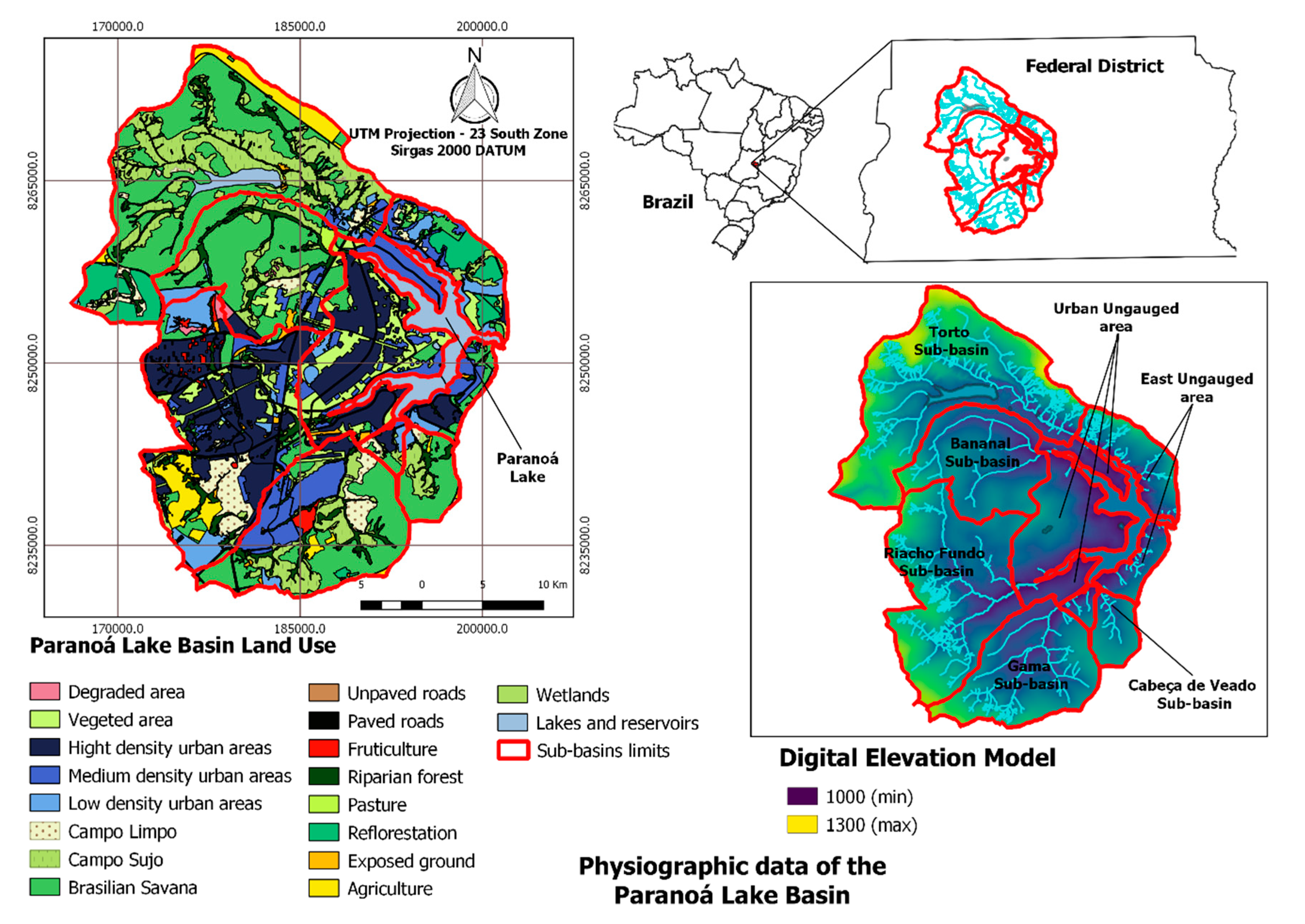
The land use provided by the Federal District Government—GDF (2010) [32] was updated manually for the year 2014 (Figure 1) using aerial images taken by the government of the Federal District obtained from the Department of Urban Development and Housing—SEDUH (2019) [33]. The typological patterns of land use adopted in modeling comprised 18 classes ranging from different types of urban, natural, and agricultural uses. The land use database is presented in

Table 2. Paranoá Lake Basin (PLB) land use.

Land Use	Area (km2)	(%)
Campo Sujo 1	123.39	12.05
Campo Limpo 1	37.89	3.70
Cerrado 2—Brazilian Savana	276.77	27.02
Degraded area	3.84	0.37
Exposed soils	7.79	0.76
Pasture	2.24	0.22
Wetlands	15.36	1.50
Water—lakes/reservoirs	46.68	4.55
Paved roads	23.19	2.26
Reforestation—eucalyptus	36.25	3.54
Agriculture	34.96	3.41
Low-density urban area	48.23	4.71
Medium-density urban area	87.85	8.57
High-density urban area	146.69	14.32
Fruticulture	6.73	0.65
Forest	62.08	6.07
Vegetated area	63.69	6.22
Unpaved roads	0.84	0.08
TOTAL	1024.47	100.00

¹ Phytophysiognomy of the Cerrado. ² Cerrado—generic Brazilian savana.

.

The digital elevation model used for the delimitation of hydrographic basins was built in this work from topographic data of contour lines with equidistance of five meters, obtained from Federal District Government—GDF (2010) [32]. The topographic data consisted of contour lines that cover the entire Federal District, as this work the area of the PLB was defined to build the Digital Elevation Model (DEM). The altitude varies from 1000 m at the level of the lake where the lowest point is, to around 1300 m in the highest region.

The classification of the PLB, according to the type of soil, took place in the first stage according to that adopted by EMBRAPA (Brazilian Agricultural Research Corporation), through an update of the cartography base of the pedology of the Federal District carried out by Reatto et al. (2004) [34]. Then, compatibility was found between the database developed by the author and that developed by Lima et al. (2013) [35], which aimed to apply the SWAT model to the Cerrado biome.

3.2. Hydro-Meteorological Data

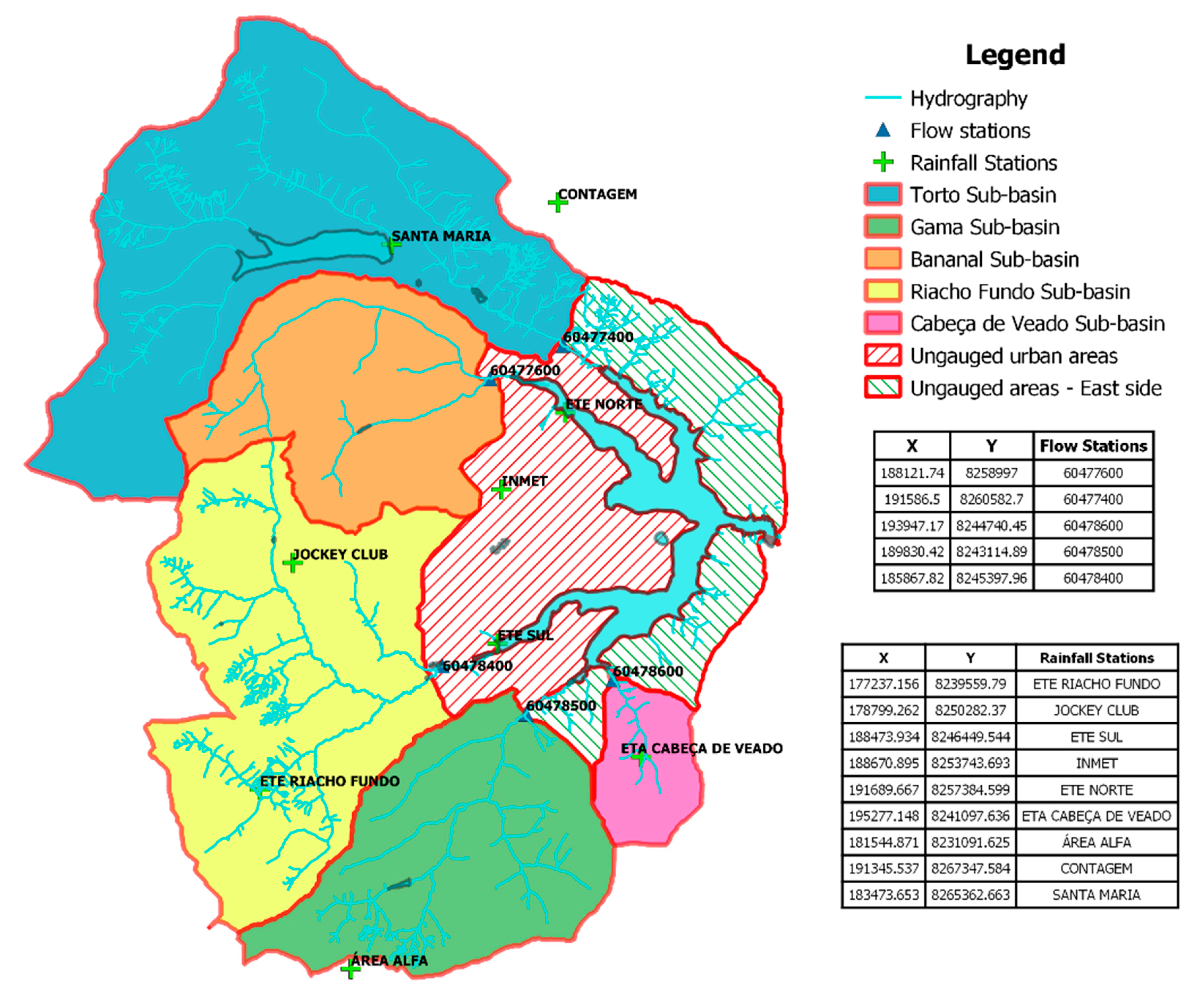
The SWAT model requires 5 types of weather data as input, these being rainfall, max and min temperatures, solar radiation, wind speed, and air humidity. The rainfall data used were obtained from 9 rainfall stations operated by CAESB (Environmental Sanitation Company of the Federal District), located alongside PLB, besides the meteorological station operated by INMET (Brazilian Meteorological Institute) from which the other meteorological input data were obtained. Another dataset necessary for the adjustment steps of the model were the flows monitored in the Paranoá Lake affluent sub-basins. The CAESB provided this dataset. The location of these monitoring stations is shown in Figure 2. The data used in this study are daily data spanning from 1982 to 2017.

Table 3. Used databases.

SWAT Input Data
Database	Parameters	Period	Region	Source
Climate data (daily)	Rainfall	1979–2017	Bananal River	CAESB
			Gama River
			Riacho Fundo River
			Torto River
			Cabeça de Veado River
Climate data (daily)	Rainfall	1979–2017	PLB	INMET
	Temperature
	Relative humidity
	Solar radiation
	Wind
Climate data (monthly)	Evaporation	1982–2017	PLB	UnB station (University of Brasilia)
Soil data (30 m × 3 m)	Soil	---	PLB	EMBRAPA
Elevation (topography) (30 m × 30 m)	(x,y,z) coordinates,	---	Federal	DEM build from GDF (2010) [32]
	contour lines		District
Land use (30 m × 30 m)	Photogrammetric survey of the Federal District	2014	Federal	GDF (2010) [32], updated by authors from aerial images from SEDUH (2019) [33]
			District
Flow Calibration Data
Database	Parameters	Period	Region	Source
Gauge data (daily)	Water discharge data	1982–2017	Bananal River	CAESB
			Torto River
			Gama River
			Riacho Fundo River
			Cabeça de Veado River
Additional Paranoá Lake Water Balance Data
Database	Parameters	Period	Region	Source
Sewage data (weekly)	Wastewater discharge data	1982–2017	WTP North	CAESB
			WTP South
Storage area curve	Bathymetry	2003	Paranoá Lake	CAESB

shows the SWAT input data.

3.3. Paranoá Lake Data

Another dataset necessary for the preparation of the study is related to Paranoá Lake, such as the storage area curve and the other flows that enter the lake. The storage area curve was obtained through the management study of Paranoá Lake [30], and the other flows into the lake can be differentiated as to their origin. The first consist of effluents from the Brasília North and Brasília South wastewater treatment plants (WTPs) that are discharged into the lake. The second is associated with ungauged areas, and for that reason their flows were estimated through the specific flow of areas modeled with the SWAT. The choice of areas took into account similar characteristics with ungauged areas such as land use. A brief resumé of all datasets used to build this study is shown in Table 3.

A likely source of lake water balance error is the outflows from the lake, consisting mostly by water released through the power generation turbines and, during the rainy season, the water released through the spillway controlled by sluice gates. The flow through the turbines is not gauged and is estimated by the amount of power generated by the 4 turbines, including 3 of them that have been working for more than 50 years. The dam was built in 1960 and the spillway/sluice gate equations had never been properly checked.

3.4. Hydrological Modeling with SWAT

SWAT is a versatile watershed model capable of modeling various processes from rain-flow to plant growth [36]. It is recognized as a model that is focused on ungauged river basin analysis [13], mainly because of its components that simulate plant growth, pesticides, and nutrients, but it is appropriate in the analysis of the impacts on the basin due to changes in land use and land cover, including the expansion of urban areas. The equation governing the hydrological components in the SWAT model is as follows [13,36]:

$$S{W}_t=S{W}_0+{\displaystyle \sum }_{t=1}^t\left(R_t-Q_t-E{T}_t-P_t-Q{R}_t\right)$$

(1)

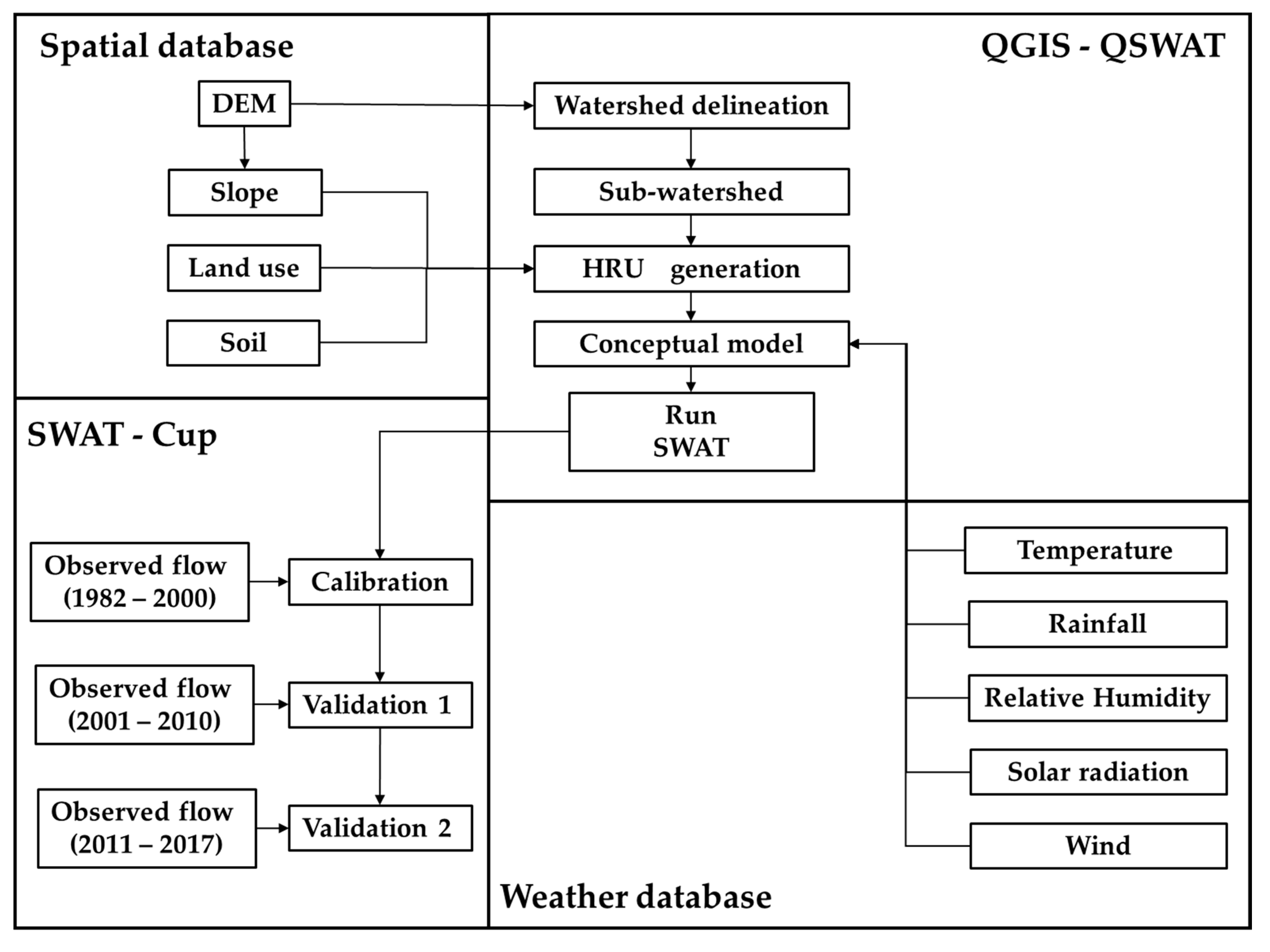
where $S{W}_t$ is the water contained in the soil at the end of the day, $S{W}_0$ is the initial amount of water contained in the soil, t represents the time in days, $R_t$ is the precipitation, $Q_t$ is the runoff, and $E{T}_t$ is evapotranspiration. $P_t$ is the percolation and $Q{R}_t$ is the return flow. All components of equation 1 are in millimeters. The general methodology used in modeling the Paranoá Lake tributary sub-basins is presented in Figure 3.

The study started with the construction of the physical database of the sub-basins that would be modeled. In QGIS/QSWAT, the physical information of the basin was loaded, and the physical model of each sub-basin was built, going through the stages of delineation of the drainage area, creation of sub-basins, and generation of HRU. The next step consisted of integrating climatic data into the physical model and, finally, we ran the SWAT model using 3 years of data from the weather database as the model’s warmup, from 1979 to 1981, for all simulated sub-basins, except for the Gama River sub-basin, which was from 1982 to 1984.

After the initial simulation of the sub-basins affluent to Paranoá Lake, we began adjustments in the sub-basins. For this, steps of sensitivity analysis, calibration, and validation were implemented. It is worth mentioning that for the validation step, we chose to perform it in two stages, the first performed from 2000 to 2010, and the second performed from 2001 to 2017.

3.5. Sensitivity Analysis, Model Performance Evaluation, Calibration and Validation, and Uncertainly Analysis

For reasonable simulations, most of the hydrological models need a certain degree of adjustment so that the results produced by the model present a high degree of agreement with the actual monitored data and thus are able to support analysis of scenarios and/or other studies from which its results serve as input data [37]. For this reason, model adjustment steps such as model calibration are very important in modeling studies.

In this study, we conducted a sensitivity analysis to find the most sensitive parameters for flow adjustment, model calibration using data from 1982 to 2000, and model validation in two stages—the first using data from 2001 to 2010 and the second using data from 2001 to 2017. With the model calibrated and verified, we performed uncertainty analysis.

Sensitivity analysis was a preliminary step to model calibration and validation. After the initial modeling of the basins, we selected a group of parameters with the greatest impact on the hydrological components simulated by the SWAT model. We sought to investigate works performed both worldwide [13,16,17] and in Brazil [17,38,39]. In the SWAT-Cup, the parameters can be changed in 3 different ways: the first is the relative change (r__)—in this method the parameter value is multiplied by a given value. The second is substitution (v__)—in this method, the parameter value is replaced by a new value each round. Finally, the third method is changing the addition (a__), wherein the value of the parameter is added by a given value [40]. The parameters selected for the sensitivity analysis are shown in

Table 4. Soil and Water Assessment Tool (SWAT) parameters (absolute values) used in sensitive analysis.

Parameter	Description	Lower Bound	Upper Bound	Process
CN2	Soil conservation service runoff curve number for moisture condition II	35	98	Runoff
ESCO	Soil evaporation compensation factor	0	1	Evapotranspiration
CANMX	Maximum canopy storage	0	100	Evapotranspiration
GW_REVAP	Groundwater “revap” coefficient	0.02	0.2	Evapotranspiration
ANION_EXCL	Fraction of porosity (void space) from which anions are excluded	0.01	1	Soil
SURLAG	Surface runoff lag coefficient	0.05	24	Groundwater
SOL_Z	Soil depth (mm)	0	3500	Soil
SOL_AWC	Available water capacity of the soil layer (mm/mm soil)	0	1	Soil
SOL_K	Satured hydraulic conductivity (mm/h)	0.05	2000	Soil
SOL_BD	Moist bulk density	0.9	2.5	Soil
ALPHA_BNK	Baseflow alpha factor for bank storage	0	1	Channel
ALPHA_BF	Baseflow alpha factor (days)	0	1	Groundwater
GW_DELAY	Groundwater delay time (days)	0	500	Groundwater
GWQMN	Threshold depth of water in shallow aquifer required for return flow to occur (mm H2O)	0	5000	Groundwater
REVAPMN	Threshold depth of water in the shallow aquifer for “revap” or percolation to the deep aquifer to occur (mm H2O)	0	500	Groundwater
GWHT	Initial groundwater height	0	25	Groundwater
SHALLST	Initial depth of water in the shallow aquifer (mm)	0	50,000	Groundwater
DEEPST	Initial depth of water in the deep aquifer (mm)	0	50,000	Groundwater
CH_N2	Manning’s “n” value for the main channel	−0.01	0.3	Channel water routing
CH_K2	Effective hydraulic conductivity in main channel alluvium	−0.01	500	Chanel water routing

.

With the set of parameters selected for the sensitivity analysis (Table 4), we used the SWAT-Cup tool [40], an interface that allows for the performance of various analyses with the results provided by the SWAT model, in order to calibrate the Paranoá Lake sub-basin models. The method used in the sensitivity analysis of the parameters and calibration of the model was the SUFI-2 [24,25,26,41,42,43]. This method has been used to analyze the sensitivity of parameters and calibration in basin modeling [44,45,46] and has been indicated to have better computational performance in complex distributed hydrological models, besides also having good accuracy in the estimates [24].

On the basis of a Bayesian framework, the SUFI-2 method determines uncertainties through the sequential and fitting process. In SUFI-2 (Figure 4), several iterations for updating the estimates of unknown parameters are required to achieve the final estimates. In this method, parameter uncertainties account for different possible sources, including model input, model structure, parameters, and observed data for calibration and validation purposes. An objective function needs to be defined before uncertainty analysis and assigned with a required stopping rule [37]. The P-factor, the percentage of observed data bracketed by 95% prediction uncertainty (95PPU), is used to quantify the degree of all uncertainties. The 95PPU is calculated at the 2.5% and 97.5% levels of the cumulative distribution of output variables through the Latin hypercube sampling method [42,43,44]. The R-factor is another index to quantify the strength of a calibration and uncertainty analysis and it reflects the average thickness of the 95PPU band divided by the standard deviation of the measured data. If the R-factor is large, the ranges of parameters are larger than the optimal parameter ranges and more parameter uncertainties will remain. Usually, a value of less than 1 is a desirable result for the R-factor [25]. Hence, a balance between these two factors has to be monitored while decreasing parameter uncertainty, with the ratio of P-factor and R-factor being able to be used to evaluate the strength and goodness of fit of uncertainty analysis. When acceptable P- and R-factors are obtained, the reduced parameter uncertainty ranges are the preferred ones [41]. Theoretically, a P-factor of 1 and R-factor of 0 indicate that the simulation exactly corresponds to the measured data. However, R-factor values < 1.5 are considered satisfactory [41,43].

The SUFI-2 method assumes a large parameter uncertainty (or physically meaningful range) to ensure the observed data fall into the 95PPU for the first iteration and decreases the uncertainty while monitoring the P-factor and R-factor for the next several iterations. The goal of the SUFI-2 method is to search for bracketing most of the observed data with the smallest possible uncertainty band. These two measures can also be used to evaluate the performance of other uncertainty analysis methods. Parameters are then updated with new ranges, which are always centered around the values of the optimal parameter set that leads to the best simulation. The major procedures of SUFI-2 are shown as follows [22,40,42,44].

The model performance analysis was performed by evaluating the generated results by SWAT. For this analysis, two different metrics were adopted [45], which are the percentage bias (PBIAS) and the Nash–Sutcliffe coefficient (NSE), which were used to evaluate the mathematical definitions of each of the metrics used in the study; these are shown below:

$$\mathrm{PBIAS}=\left[\frac{{\sum }_{i=1}^n\left(Q_i^{obs}-Q_i^{sim}\right)·100}{Q_i^{obs}}\right]$$

(2)

$$\mathrm{NSE}=1-\left[\frac{{\sum }_{i=1}^n{\left(Q_i^{obs}-Q_i^{sim}\right)}^2}{{\left(Q_i^{obs}-Q_i^{mean}\right)}^2}\right]$$

(3)

where Q is the discharge.

The calibration process was carried out with three iterations [22,24], each with 1900 runs. This number was adopted through considering a reasonable 100 runs multiplied by the number of parameters. After each iteration, the intervals of each parameter were updated, taking into account the feasible physical limits for the studied basins, and then a new iteration was performed. After 3 iterations, the intervals for each parameter were applied in the following steps, the first validation stage (2001–2010) and the second validation stage (2011–2017), as recommended in the literature for evaluation of the results [25,40,42].

3.6. Paranoá Lake Water Balance

The necessary dataset for the Paranoá Lake water balance computation were inlet flows, precipitation, evaporation, and outflows. The flow generated by modeled sub-basins with the SWAT provided the inlet flows to Paranoá Lake, comprised of streamflow and groundwater contribution, from the tributary sub-basins. Precipitation was estimated based on the series of monitored data provided by INMET and CAESB and evaporation was estimated on the basis of data monitored by UnB stations, measured with class A tank.

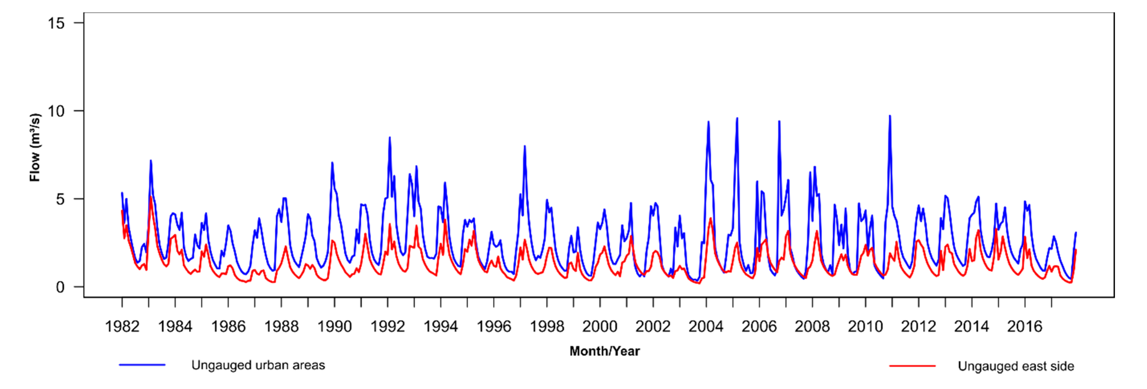
The ungauged areas, about 20% of the basin area, have a relevant contribution in determining the water balance of Paranoá Lake. These areas have 2 types of land use, urban and preserved. Thus, we chose to estimate the contribution flow of these areas by applying the specific flow of the sub-basins with similar characteristics modeled with the SWAT [6]. Thus, the contribution flow from the ungauged urban areas of Brasília, as well as from the cities Lago Norte and Lago Sul, were estimated on the basis of the specific flow of the Riacho Fundo sub-basin, the basin with the highest percentage of urban occupation contributing to Paranoá Lake. In turn, the contribution of the ungauged eastern side of Paranoá Lake was estimated on the basis of the specific flow of the Gama sub-basin due to similarities concerning land use and occupation. There are also two wastewater treatment plants that release their effluents into Paranoá Lake. These plants are operated by CAESB, which provided the data released on Paranoá Lake during the period studied.

The estimate of the water balance for Paranoá Lake was based on the continuity equation, given by

$$S_{\left(t+1\right)}=S_{\left(t\right)}+Q_{inflow\left(t\right)}+P_{lake\left(t\right)}+G_{net\left(t\right)}-Q_{outflow\left(t\right)}-E_{reservoir\left(t\right)}+{ϵ}_{\left(t\right)}$$

(4)

where the terms $S$ and $S_{\left(t+1\right)}$ represent the storage at time t and at time $t+1$, $Q_{inflow\left(t\right)}$ is the lake inlet flow, $P_{lake\left(t\right)}$ is the precipitation rate direct in the lake, $G_{net\left(t\right)}$ is the groundwater contribution rate, $Q_{outflow\left(t\right)}$ is the outflow, and $E_{reservoir\left(t\right)}$ is the evaporation rate. The last term, ${ϵ}_{\left(t\right)}$, represents the uncertainties in the water balance arising from the process of acquisition and manipulation of data in addition to unrecorded portions.

4. Results

The analysis carried out considered the availability of monitored hydrological data in the basin, thus using climatic and hydrological data for approximately 30 years. The results generated by the SWAT model for each sub-basin are presented below.

4.1. Gauged Sub-Basins: Modelling, Sensitivity Analysis, and Calibration Uncertainty Analysis

4.1.1. Default Simulation and Sensitivity Analysis

The initial results generated by the SWAT model for each sub-basin were evaluated by the metrics adopted in this work (

Table 5. Model performance scale [46].

Performance	NSE	PBIAS (%)
Very good	0.75 $\le$ NSE $\le$ 1	PBIAS $\le$ ±10
Good	0.65 $\le$ NSE $\le$ 0.75	$\le$ ±10 PBIAS $\le$ ±15
Satisfactory	0.5 $\le$ NSE $\le$ 0.65	$\le$ ±15 PBIAS $\le$ ±25
Unsatisfactory	NSE $\le$ 0.5	PBIAS $\ge$ ±25

) and can be seen in

Table 6. Statistical results for initial simulation.

Sub-Basin	Default Simulation (1982–2017)
	NSE	PBIAS
Bananal	−1.55	3.8
Gama	−0.14	−25.6
Riacho Fundo	0.05	−18
Torto	−0.02	42.7
Cabeça de Veado	−2.93	52.8

.

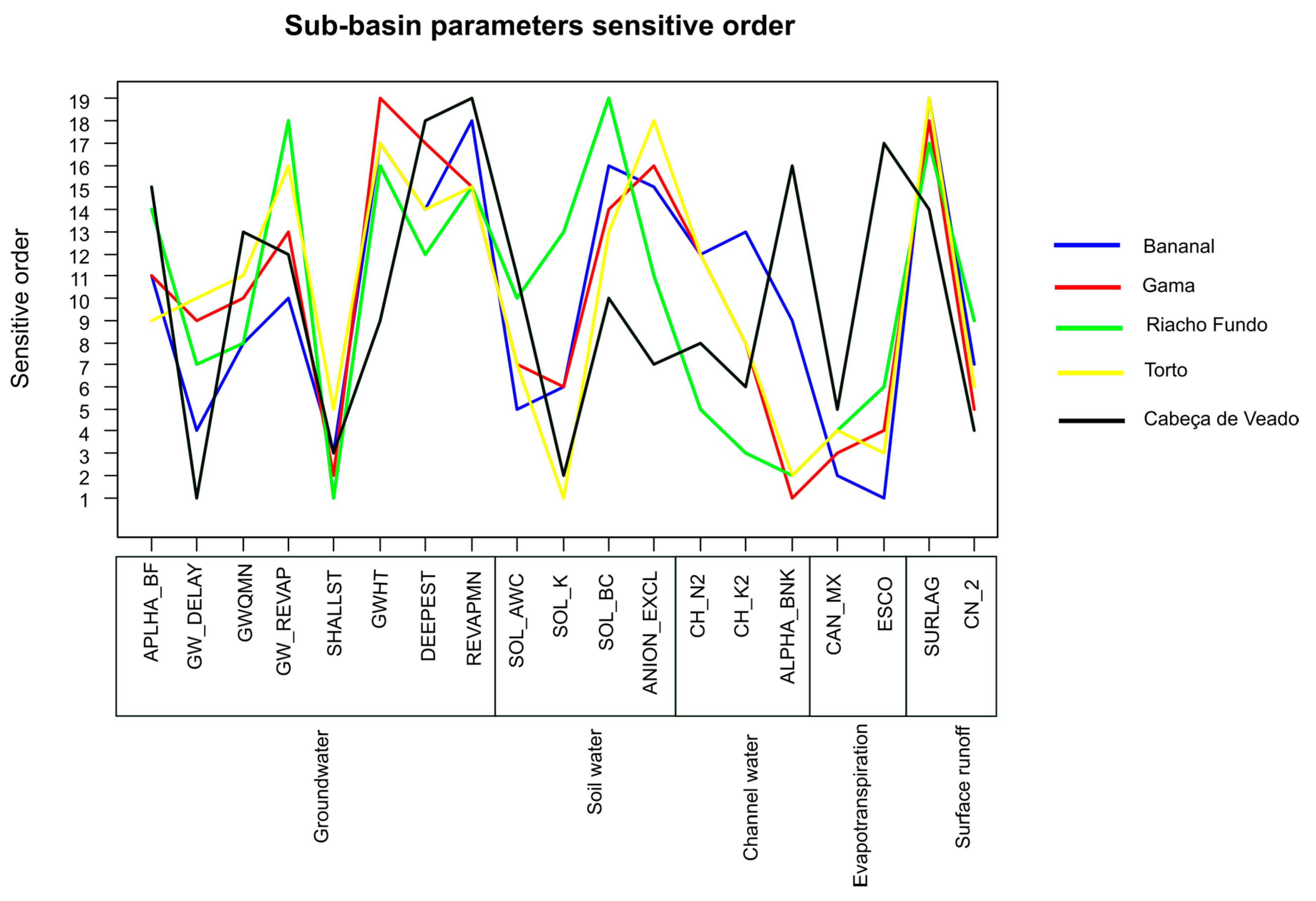
The initial results generated by the SWAT model showed the need for model adjustment. Thus, we proceeded with the sensitivity analysis of the parameters. This analysis sought to perform the ranking of the most sensitive parameters for each sub-basin (Figure 5). The x-axis shows the most sensitive parameters separated by the hydrological process, while the y-axis shows the order of sensitivity of the parameters in each of the studied basins.

The results in Figure 5 showed a tendency regarding the sensitivity of the parameters in the modeled sub-basins, with emphasis on the parameters SHALLST, GWQMN, and GW_DELAY, which are related to underground waters. Similarly, about the processes associated with water in the soil, the emphasis is given to SOL_K and SOL_AWC, with visible sensitivity in all basins except the Riacho Fundo River sub-basin. The low sensitivity of this parameter in the Riacho Fundo River sub-basin may be related to the predominantly urban type of land use.

Regarding the parameters associated with evapotranspiration, both CAN_MX and ESCO parameters showed high sensitivity, especially CAN_MX, in all simulated sub-basins, while ESCO was found to not be sensitive to Cabeça de Veado sub-basin.

As for the water routing in the channel, the three parameters (CH_N2, CH_K2, and ALPHA_BNK) showed a certain degree of sensitivity, with the parameter ALPHA_BNK showing low sensitivity in the Cabeça de Veado sub-basin.

Finally, for the runoff process, CN2 was relevant in all basins, as expected, since it directly reflects the amount of runoff generated in the basin. The most sensitive parameters in the basins studied in this work (Figure 3) were reported in other studies conducted in Brazil. The set of parameters CN2, SOL_AWC, SOL_K, SOL_Z, ESCO, and CANMX, some of the most sensitive parameters in this hydrological study also were related to sediment production in other brazilian basins [18,46]. In the Federal District, the results presented in this study corroborate other findings [27,28,29].

4.1.2. Calibration and Uncertainty Analysis

The calibration of the sub-basins was performed with three iterations each with 1900 runs, a procedure similar to that adopted in [22,24]. In each iteration, the metrics for evaluating the results of the model (NSE, PBIAS, P-factor, R-factor, 95PPU) were analyzed to observe the reduction of uncertainty associated with the calibration of the parameters, and we noticed that more than three iterations did not provide a significant improvement in the results. Moreover, at each iteration, the limits of the parameters were updated, always taking care to keep them within the physical limits that are representative of the modeled sub-basins.

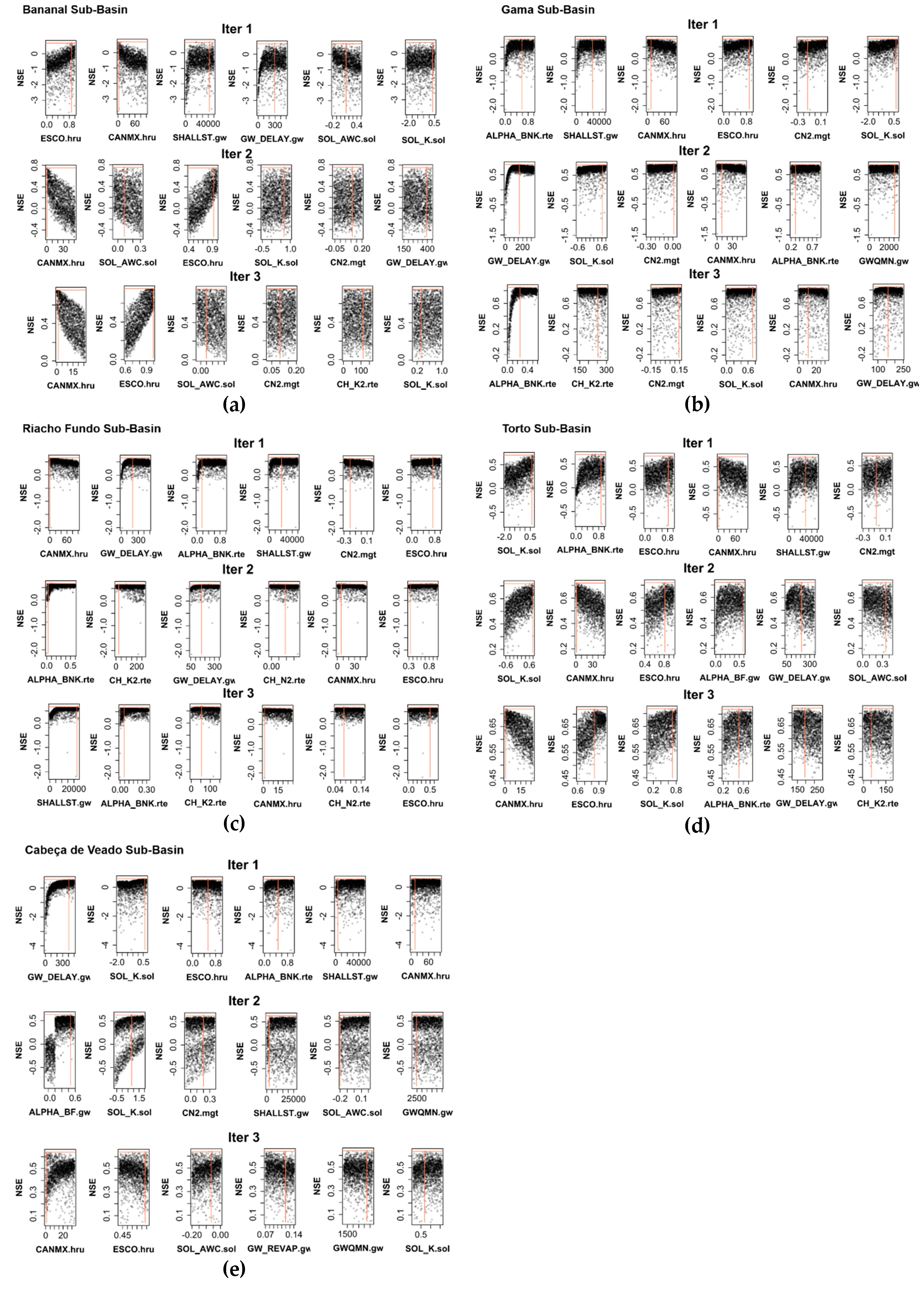
The trends of each parameter were observed in each iteration towards the best NSE values (Figure 6), so that as the intervals of each parameter were updated in each iteration, the NSE values were also optimized, showing the increase in NSE values throughout the iterations. The increase in the NSE over the iterations showed a reduction in the uncertainty in the results of the model since at each iteration the upper and lower limits of each parameter were reduced and therefore the space of solutions that gives optimal or sub-optimal solutions was better delimited.

Analyzing the graphs of the optimized parameters, we noticed that with each iteration the sensitivity parameter order changed; this happened because when a given parameter found its region of optimal solutions, the alteration of other parameters started to generate impacts more significant in the calibration of the flows of each sub-basin.

In the results shown in Figure 6, we observed that the applied methodology provided effective results for the simulation of the basins seeking to reduce the degree of uncertainty regarding the model parameters. This behavior can be seen with the NSE values obtained, since the higher the NSE, the lower the uncertainty and the greater the adjustment of the simulated datasets to those observed.

With the results, we observed that the greatest uncertainties were associated mainly with five processes, described below and contemplated in Figure 5 and Figure 6.

• The use and cover of the soil evidenced by CN2, the parameter of impact on the runoff generated in the sub-basins.
• The evapotranspiration represented by the parameters CAN_MX and ESCO that are associated with water stored in the vegetation canopy and the water evaporation capacity of the soil.
• The flow of soil water given by the parameters SOL_AWC and SOL_K with the water available in the soil and the conductivity of the saturated soil, respectively.
• The parameters associated with groundwater represented by the parameters GW_DELAY and SHALLST, with these being the groundwater lag and the initial height of the water in the deep aquifer, respectively.
• Finally, the parameters associated with the channel water routing, represented by CH_N2, CH_K2, and ALPHA_BNK, which are Manning n’s value for the channel, effective hydraulic conductivity in the main channel, and the base flow alpha factor for bank storage, respectively.

After the model calibration for the sub-basins, we observed a considerable improvement in the model evaluation metrics. So, the results can still be considered satisfactory (

Table 7. Summary of metrics for each modeled sub-basin.

Step (Period)	Metrics	Sub-Basins
		Bananal	Gama	Riacho Fundo	Torto	Cabeça de Veado
Calibration (1982–2000)	NSE	0.76	0.85	0.68	0.72	0.64
	PBIAS	−0.60	−0.80	0.40	−9.40	3.20
	P-factor	0.62	0.88	0.79	0.59	0.77
	R-factor	0.59	0.86	0.84	0.54	0.84
First Validation (2001–2010)	NSE	0.80	0.86	0.49	0.56	0.63
	PBIAS	2.00	−6.10	13.80	11.90	7.70
	P-factor	0.81	0.84	0.77	0.31	0.82
	R-factor	0.84	0.82	0.80	0.40	0.92
Second Validation (2011–2017)	NSE	0.92	0.74	0.60	0.60	0.57
	PBIAS	−2.30	−17.10	−3.30	−23.50	8.50
	P-factor	0.96	0.65	0.77	0.33	0.38
	R-factor	0.83	0.81	0.88	0.58	0.49

). The final intervals obtained for the parameters used in the calibration process after the third iteration of the SUFI-2 algorithm are shown in

Table A1. Range values for calibration in modelled sub-basins.

Parameter	Bananal		Gama		Riacho Fundo		Torto		Cabeça de Veado
	Min	Max	Min	Max	Min	Max	Min	Max	Min	Max
r_CN2.mgt	0.03	0.20	−0.14	0.16	−0.14	0.16	−0.2	−0.025	0.06	0.34
v__ALPHA_BF.gw	0.2	0.7	0.40	0.80	0.6	1	0.29	0.9	0.09	0.84
v__GW_DELAY.gw	270	446	77	246	71	257	126	293	325	500
v__GWQMN.gw	11,232	33,699	1281	3842	2490	4567	1803	4257	1173	3724
v__GW_REVAP.gw	0.07	0.15	0.00	0.10	0.06	0.14	0.01	0.09	0.07	0.14
v__ESCO.hru	0.60	1.00	0.60	0.91	0.002	0.67	0.6	1.00	0.42	0.71
v__ALPHA_BNK.rte	0.28	0.60	0.02	0.59	0	0.32	0.2	0.76	0.36	0.66
r__SOL_AWC().sol	−0.03	0.21	0.20	0.41	−0.16	0.3	0.17	0.52	−0.20	0.00
r__SOL_K().sol	0.08	1.00	0.00	0.80	−1.8	−0.93	0.06	0.8	0.09	1.59
r__SOL_BD().sol	−0.50	−0.67	−0.78	−0.48	−0.75	−0.6	−0.6	−0.33	−0.93	−0.63
v__SHALLST.gw	22,284	40,762	22,030	37,633	0	23,592	28,824	50,000	0	14,638
v__GWHT.gw	2	12	4.52	13.51	7	18	0	7.2	4.30	17.62
v__DEEPST.gw	13,727	41,183	18,906	32,550	35,204	50,000	0	16,182	10,607	31,823
v__ANION_EXCL.sol	0.4	1	0.67	1.00	0.01	0.43	0.5	0.98	0.29	0.73
v__REVAPMN.gw	7	198.5	22	174	95	285	0	178	158	474
v__SURLAG.bsn	9	19	13	20	0.05	8.80	13.30	20.5	0.44	10.84
v__CANMX.hru	0	26	0.00	32.90	0	29	0	27	0	33
v__CH_N2.rte	0.1	0.24	−0.01	0.12	0.04	0.15	0.05	0.18	0.05	0.16
v__CH_K2.rte	−0.01	162.3	142	302	−0.01	150	−0.01	190	83	250

, as well as the determination of each water balance (

Table A2. Water balance sub-basin processes for modeled sub-basins.

Hydrologic Process	Sub-Basins
	Bananal		Gama		Riacho Fundo		Torto		Cabeça de Veado
	(mm)	(m3/s)	(mm)	(m3/s)	(mm)	(m3/s)	(mm)	(m3/s)	(mm)	(m3/s)
Precipitation	1337.2	5.33	1392.2	6.03	1449.4	9.81	1271	9.41	1438.3	9.41
Evapotranspiration	782.5	3.12	894.8	3.87	790.9	5.35	863.4	6.39	934.8	6.39
Surface runoff	90.83	0.36	138.06	0.6	404.68	2.74	31.94	0.24	42.09	0.24
Lateral flow	60.57	0.24	87.13	0.38	11.65	0.08	137.9	1.02	104.77	1.02
Percolation to the shallow aquifer	410.49	1.64	270.26	1.17	270.26	1.17	256.47	1.9	373.06	1.9
Revap from shallow aquifer	227.66	0.91	85.15	0.37	85.15	0.37	74.94	0.55	33.31	0.2
Return flow	227.66	1.56	256.74	1.11	256.74	1.11	243.65	1.8	354.41	1.8
Recharge to deep aquifer	390	0.08	13.51	0.06	13.51	0.06	12.82	0.09	18.65	0.09
Area (km2)	125.79		136.55		213. 41		233.4		30

) process for the gauged sub-basins.

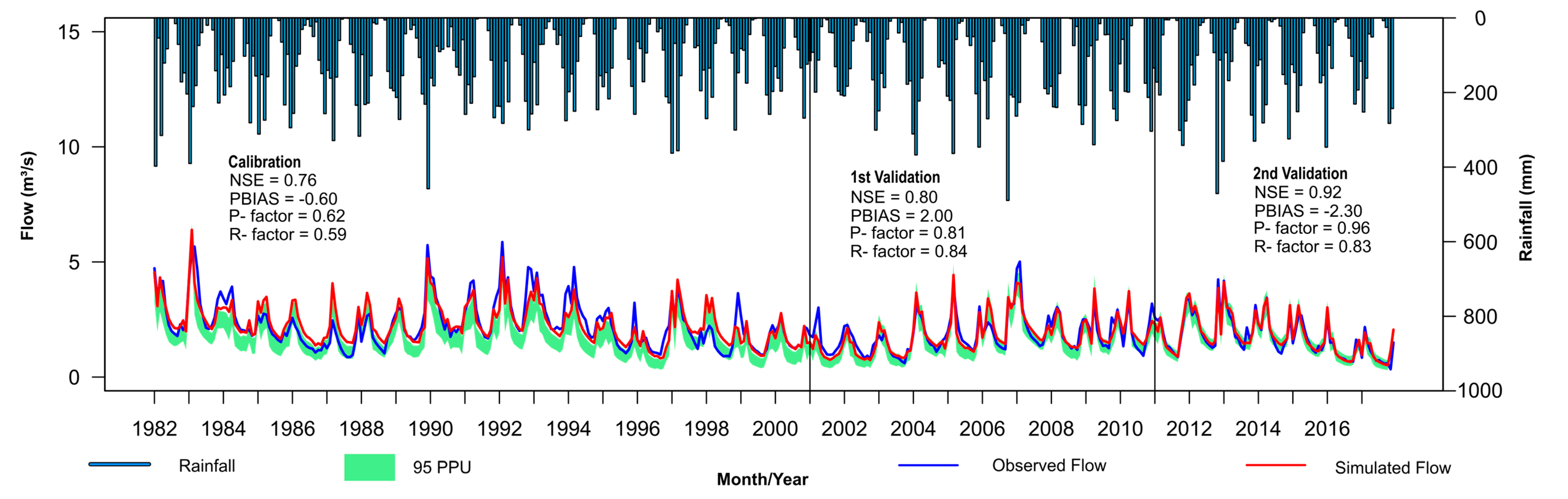
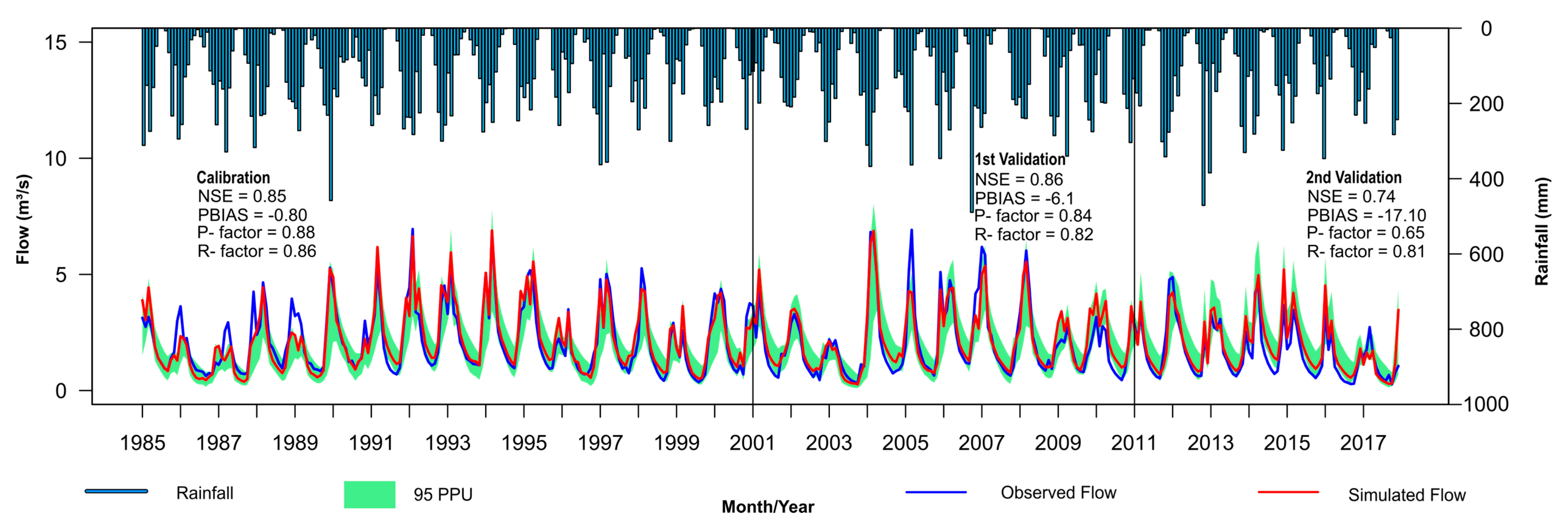
In the Bananal sub-basin (Figure 7), the SWAT model performed well in all stages of analysis. We observed that the range of parameters obtained in the third iteration was able to obtain good results also for the first and second validations. Similarly, this occurred in the Gama sub-basin (Figure 8). These sub-basins have high natural vegetation cover due to the implementation of preservation policies adopted in the PLB. Thus, it is possible to observe the good performance of SWAT in the hydrological simulation of natural environments and without major anthropogenic interventions.

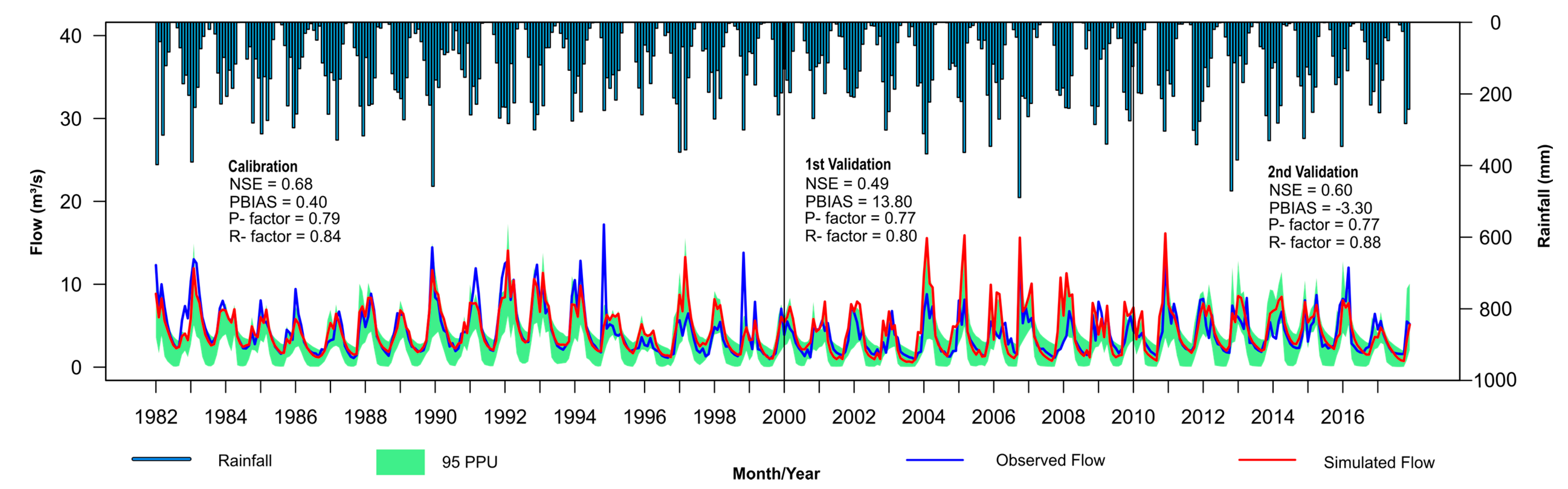
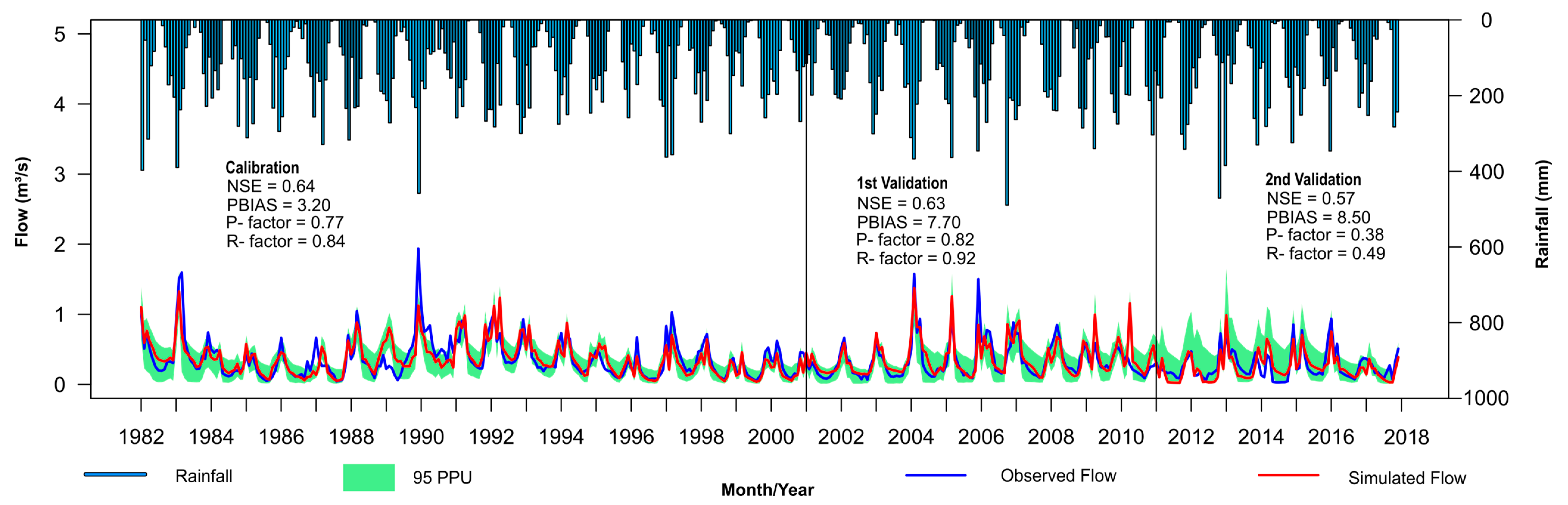
The SWAT model performed well in modeling the Riacho Fundo Basin (Figure 9), a fact that deserves mention for two main reasons. The first is associated with the fact that this basin was the target of major changes in land use between the 1980s and 2000s, going from predominantly agricultural to a high degree of urbanization. The second denotes the ability of the SWAT model to represent hydrological processes in densely urbanized basins, even though it is a model developed for hydrological analysis of rural basins. However, it is still observed that the modeling performance for the calibration stage of this sub-basin was below sub-basins such as Bananal, Gama, and even Torto that did not have significant changes in their land use. These differences are associated with the reasons already mentioned above and also with problems associated with the uncertainties in the flow-monitoring station reported by CAESB.

In this sense, it is worth noting that the dynamics of water flow in urban basins occur more intensely when taking into account the runoff that occurs in different ways depending on the type of soil cover and the degree of urbanization to which the basin may be subjected. Therefore, studies that advance in the discretization of these patterns’ area are important to improve the model and, consequently, its capacity for the hydrological representation of the basin. We consider this an important factor in the Riacho Fundo sub-basin, since, despite the high degree of urbanization, different patterns may be present in the basin and the typological patterns presented in the SWAT model take into account only three categories, which are areas of low, medium, or high urban density. Factors such as these may explain the drop in the model’s performance in the representation of the Riacho Fundo sub-basin, especially when taking into account other factors such as the uncertainties associated with the flow monitoring and the modeling process.

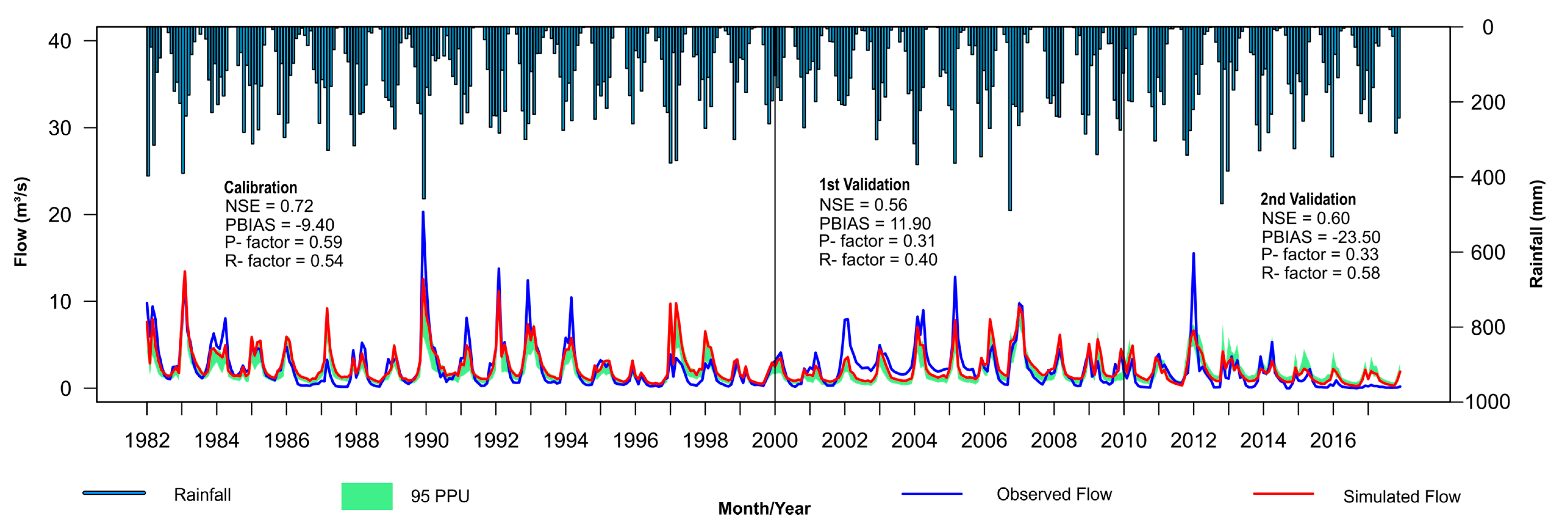
In the Torto sub-basin (Figure 10), there is a decrease in the model efficiency for the first (NSE = 0.56; PBIAS = −11.90) and second validation periods (NSE = 0.60; PBIAS = −23.50) in comparison with the calibration period (NSE = 0.72; PBIAS = −9.40). It is worth mentioning that from 2013 onwards, the observed flow decreased year by year, a period that coincided with the increase in demands that have occurred since the end of the 2010s, as pointed out by [3]. The sub-basin that presented the lowest performance was the Cabeça de Veado (Figure 11), which presented a lower NSE value in calibration between the modeled sub-basins. However, even so, we see that the results obtained are reasonable and show a good simulation for the basin.

It is important to highlight that the Torto sub-basin, as well as the Cabeça de Veado sub-basin, are water supply sub-basins, and that the drop in the performance of the model can be linked to the input data of water withdrawal that occur in a monthly stage, affecting periods that do not have similar behavior to the historical average.

A summary of the results obtained for each simulated sub-basin is found in Table 7, and the detailed aspects of hydrological modeling of the gauged sub basins as range parameter values and the sub basins water balances are in Appendix A.

A general analysis of the water balance plots of the Paranoá tributary sub-basins obtained throughout the study period (

Table 8. Water balance ratios for modeled sub-basins.

Water Balance Ratios	Bananal	Gama	Riacho Fundo	Torto	Cabeça de Veado
Streamflow/rainfall	0.40	0.35	0.46	0.33	0.22
Baseflow/total flow	0.83	0.71	0.38	0.92	0.88
Surface runoff/total flow	0.17	0.29	0.62	0.08	0.12
Percolation/rainfall	0.31	0.19	0.17	0.2	0.15
Deep recharge/rainfall	0.02	0.01	0.01	0.01	0.01
Evapotranspiration/rainfall	0.59	0.64	0.55	0.68	0.78

) shows that the largest contribution impact to the flow in the river channel is from the base flow. These values are very expressive for sub-basins that have a high percentage of land use in preserved areas such as Bananal (83%), Gama (71%), Torto (92%), and Cabeça de Veado (88%). The sub-basin that had the lowest percentage of base runoff contribution to the final flow was the Riacho Fundo. Although it is still significant that the contribution of the base runoff represented only 38% of the total, explained by the high percentage of urbanization, this aspect ended up emphasizing the surface runoff process that was predominant in the sub-basin, representing 62% of the water produced in the sub-basin. This result is relevant because it shows the importance of maintaining natural areas, as once maintained, important processes for maintaining the flows in the sub-basins and, consequently, contributions to Paranoá Lake are guaranteed.

4.2. Ungauged Sub-Basins

From the results obtained through the modeling of the monitored basins, we estimated the inflow to the Paranoá Lake of the unmonitored areas on the basis of the specific flow of areas with similar characteristics, i.e., flow per area. The contribution of the ungauged urban area was determined on the basis of the modeled results for the Riacho Fundo sub-basin, and the contribution of the east side of the PLB was determined on the basis of the modeled data for the Gama sub-basin. The determination of each water balance process of the ungauged areas can be found in Appendix A.

4.3. Paranoá Lake Inflows and Outflows

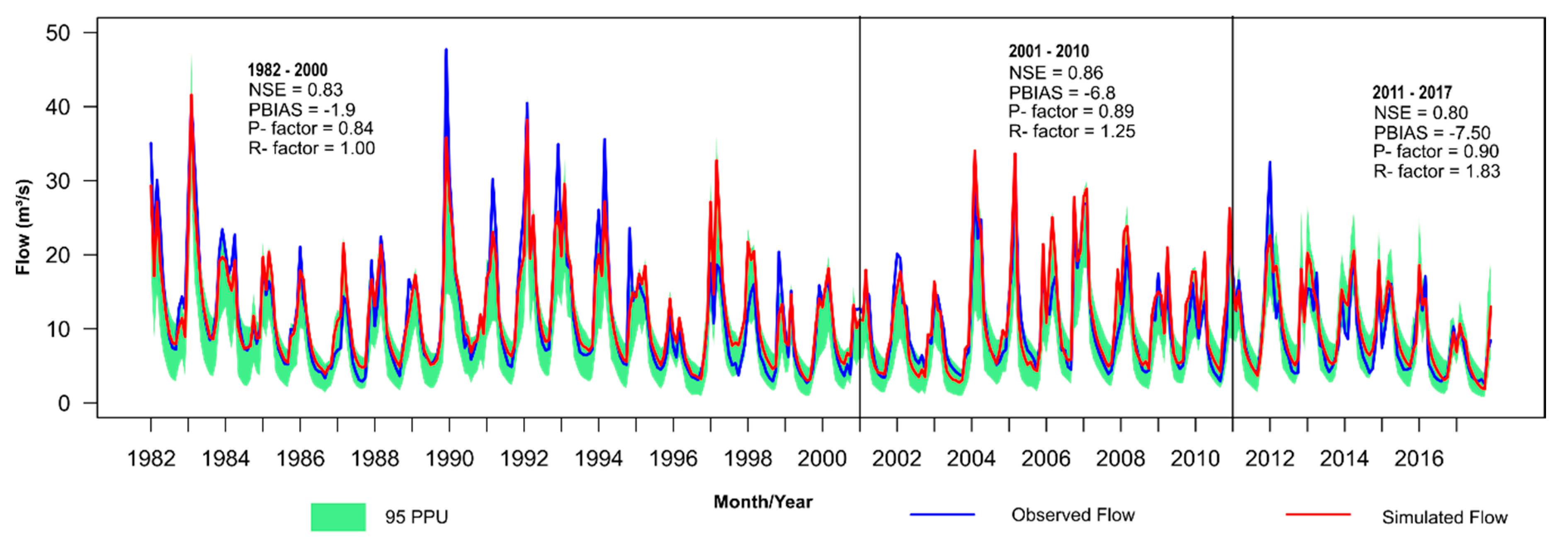
The monitored sub-basins affluent to Paranoá Lake were simulated and calibrated with the SWAT model. We performed the sum of the observed and simulated flows that contribute to Paranoá Lake and calculated the model evaluation metrics (Figure 12) in order to evaluate the results generated by the modeling process in the adjustment of the sub-basin simulations, since the calibrated flows would be used in determining the lake water balance.

The results in Figure 12 show that the SWAT model performed well in determining the flow rates of the sub-basins affluent to Paranoá Lake; this can be observed through the values of NSE and PBIAS in the three evaluated periods. The major differences, however, were in the rainy periods over the years when the model underestimated affluent flows and other years when the model overestimated affluent flows. However, when considering the evaluation periods in general, the SWAT model always underestimated the affluent flows with PBIAS of −1.9 in the calibration period, −6.8 and −7.5 in the first and second validation stages, respectively; even so, they are values that allow classification of the estimates as very good. 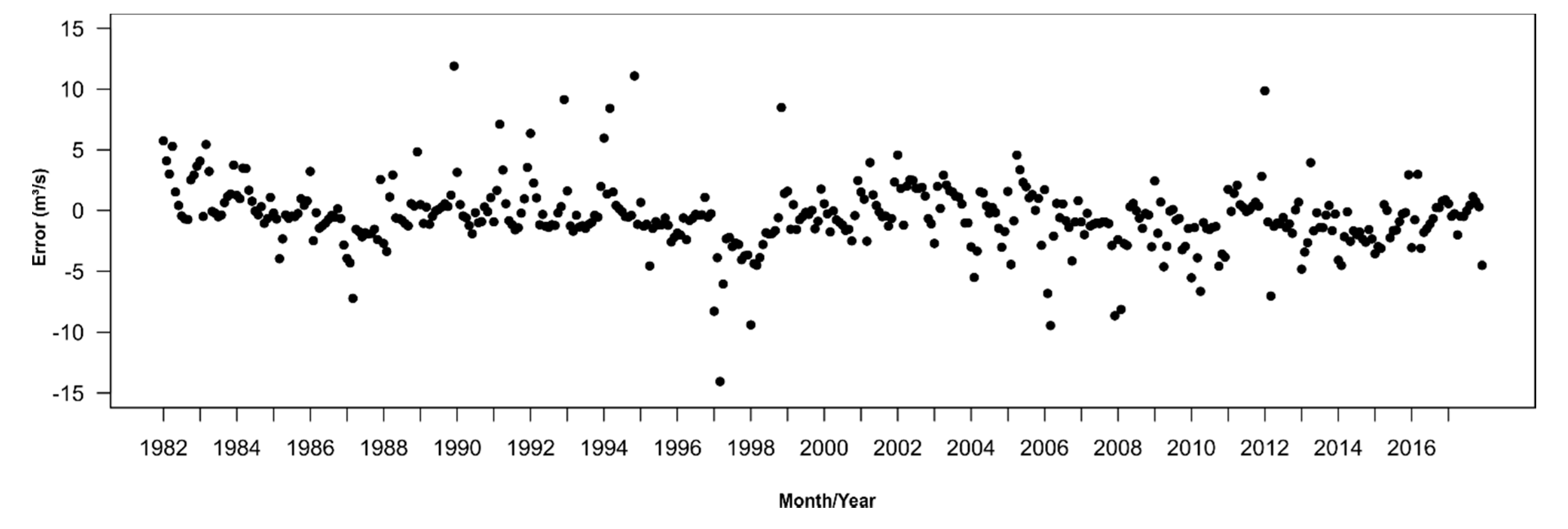The differences between the sum of observed gauged flows into Paranoá Lake and the adjusted flows generated by the SWAT model are shown in Figure 13.

We inserted the difference between the Paranoá Lake inflows from the monitored sub-basins and the calibrated flows generated by the SWAT model shown in Figure 13 in order to provide a more feasible idea of the error associated with the modeling. It was noticed that the error was concentrated in the range between ±5 m³/s; however, it can be observed that relevant errors, as observed for the rainy season in 1990 associated with higher observed flows generated by the model, had the most impact on the affluent flow of the Torto sub-basin (Figure 10). In addition to this, it is relevant to comment on the difference for the year 1997, wherein the model presented overestimated flows compared to the monitored flows.

We point out that a possible cause of the errors obtained for the years 1990 and 1997 could be the data input related to the water released from the Santa Maria reservoir, which is located in the Torto sub-basin. We believe that errors can be introduced due to the that the fact that the water withdrawal data from the reservoir must be supplied as input to the model as a long-term monthly average and not a continuous series. The reservoir has an uncontrolled spillway and no other discharge device, and thus the reservoir operation depends on the water demand, which is dynamic because it is part of an integrated multiple source system, and the use of monthly long-term averages does not effectively describe the behavior of the reservoir, impacting the simulated flow rates in the Torto sub-basin. In spite of that, we consider that this aspect does not impair the use of the model and the analysis structure developed in this work concerning hydrological aspects, but we emphasize that some attention should be paid to rainy seasons when the reservoir may behave differently from that observed in the long-term data, which can result in underestimations in extraordinary rainy seasons when the reservoir reaches its maximum capacity and spills, as well as overestimations in rainy seasons with below-average rainfall when no outflow is generated.

Even with differences such as those mentioned, the average error observed over the studied period was −0.48 m³/s, a negligible error when compared to the average tributary flow to Paranoá Lake (observed affluent flow = 11.04 m³/s; simulated affluent flow = 11.52 m³/s).

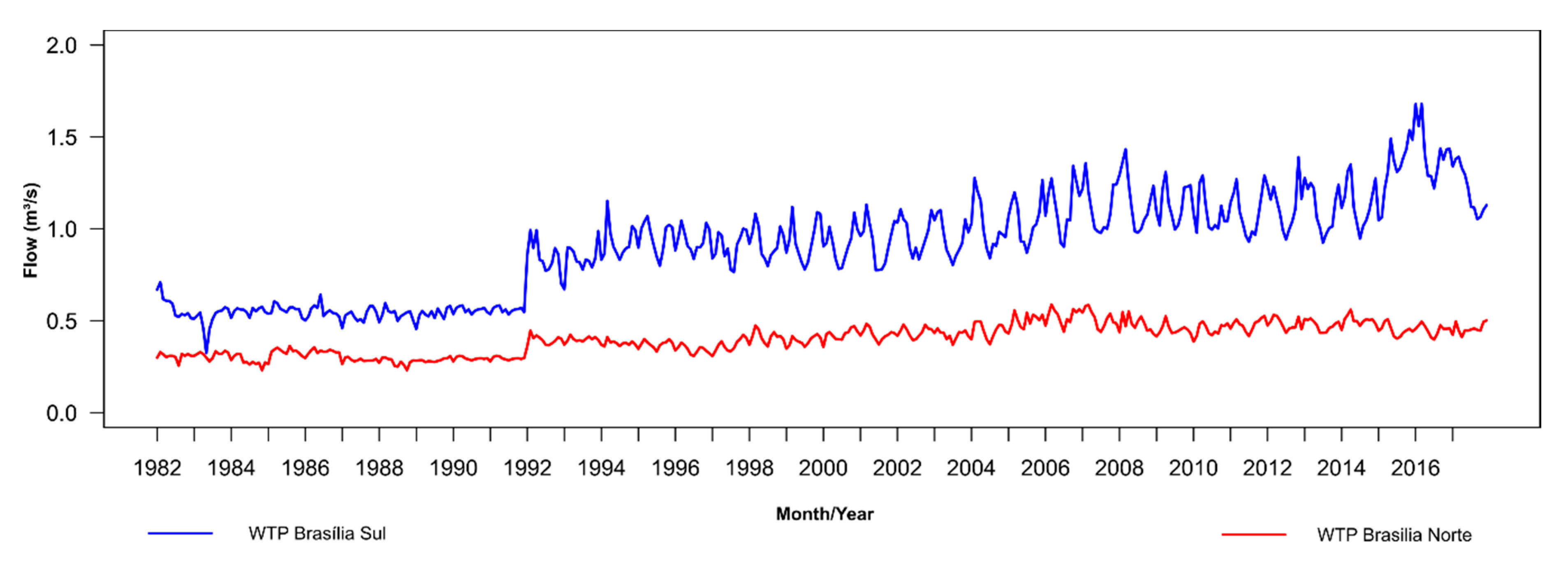
The other flows that contribute to Paranoá Lake correspond to ungauged areas (urban areas and east side, Figure 14) and the wastewater treatment plants WTP Norte and WTP Sul (Figure 15). The average contribution over a long period was 2.072 m³/s for the urban area and 1.341 m³/s for the east side.

The contribution of wastewater treatment plants is of great relevance to the lake, with flow rates higher than Cabeça de Veado sub-basin, for example. The long-term average for each one is 0.402 m³/s for WTP Brasilia Norte and 0.906 m³/s for WTP Brasília Sul. Visibly, in 1992, after improvements in sewage treatment, the stations had their capacity increased and therefore there was an increase in the flows of WTPs that were launched in Paranoá Lake, mainly of WTP Brasília Sul, the biggest treatment plant in the city of Brasília.

The system’s water losses occur through two main ways involving the outflows that result from the operation of the Paranoá Lake dam, which are divided into spillway and turbine flows. The operation of the reservoir is predominantly for power generation, which registers a historical average turbine flow of around 14.7 m³/s, the only exceptions being the lowering of the lake level for the damping of flows in rainy seasons and the opening of the spillway when the water level reaches the maximum operational level. The average historical flow is about 1.9 m³/s, with average monthly flows exceeding 50 m³/s already recorded.

4.4. Paranoá Lake Water Balance

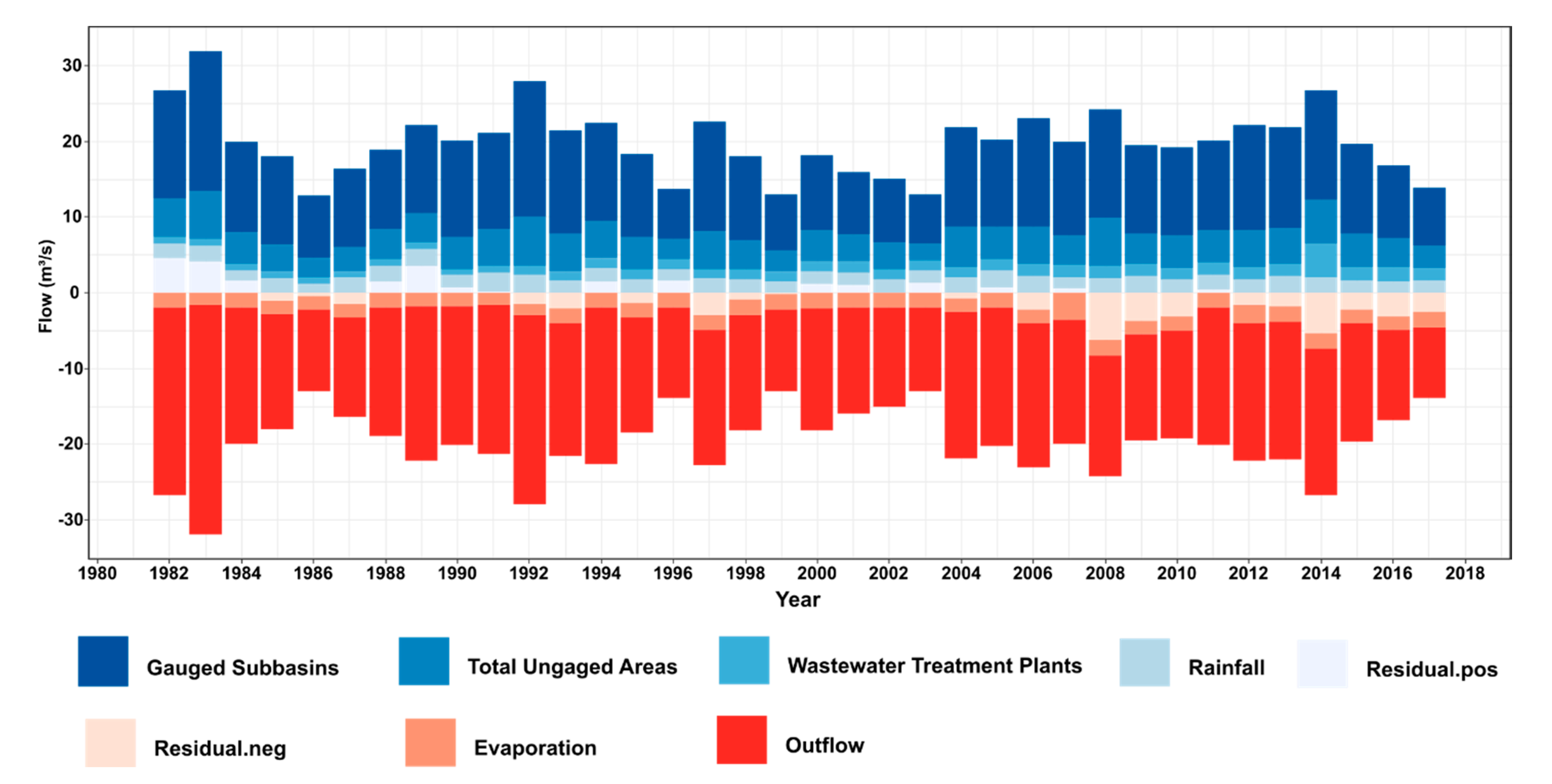
The annual water balance of Paranoá Lake (Figure 16) from 1982 to 2017 shows in 1983 the highest flow in the series, reaching about 30 m³/s. The years 1986, 1996, 1999, and 2003 presented the lowest values with values close to 13 m³/s. These years were marked by lower total rainfall throughout the basin, directly affecting the water balance of Paranoá Lake.

From 2004, there was a certain regularity in the water balance, ranging from 20 m³/s to 25 m³/s. This period lasted until the year 2014, with an approximate value of 27 m³/s. From 2015, there was a gradual decrease in the values, reaching 15 m³/s in the year 2017.

The observed residues reflect the uncertainties associated with the process of determining all input and output flows of the lake water balance. The main sources of uncertainties in the inflows for the determination of the water balance are in the inflows from ungauged areas, such as urban areas and the east side, estimated due to the extrapolation of the results obtained in the modeled basins. The uncertainty is also associated with the modeling process, which is reduced with the calibration process. Other sources of uncertainties may be associated with the outflows of Paranoá Lake. As it has an old dam, the turbine flow is estimated from the generated electricity and the spillway has no known flow-rate equation. In addition, the only measured flow after the Paranoá Lake dam is that of a fluviometric station approximately 2 km downstream and with an unstable key curve due to flow measurement difficulties in the deactivated section since 1999.

In addition to these uncertainties, there are three main sources of errors related to the storage of water in the lake. The first is associated with level measurements, a second is related to the amplitude of temperature changes that may increase and decrease the water density, and the last is associated with the bathymetry data available and the possibility of inaccurate volume determination [47]. However, there are other sources of errors that are difficult to compute such as those intrinsic to measuring instruments; the location of measuring stations, operation, and data recording; and coefficients for evaporation [7].

The long-term water balance (

Table 9. Mean water balance of Paranoá Lake (1982–2017).

Source	Inflows (m3/s)	(%)
Bananal	2.085	11.5
Gama	2.228	12.3
Riacho Fundo	4.458	24.7
Torto	2.409	13.3
Cabeça de Veado	0.337	1.9
Urban ungauged areas	2.072	11.5
East side ungauged areas	1.341	7.4
WTP Brasilia Norte	0.402	2.2
WTP Brasilia Sul	0.906	5.0
Rainfall	1.835	10.2
Total	18.073	100.0
Sink	Outflow (m3/s)	(%)
Dam—turbined flow	14.771	81.7
Dam—spillway flow	1.950	10.8
Evaporation	1.352	7.5
Total	18.073	100.0

) with average inflows and outflows of the Paranoá Lake calculated over the studied period corresponded to a flow of 18.073 m³/s.

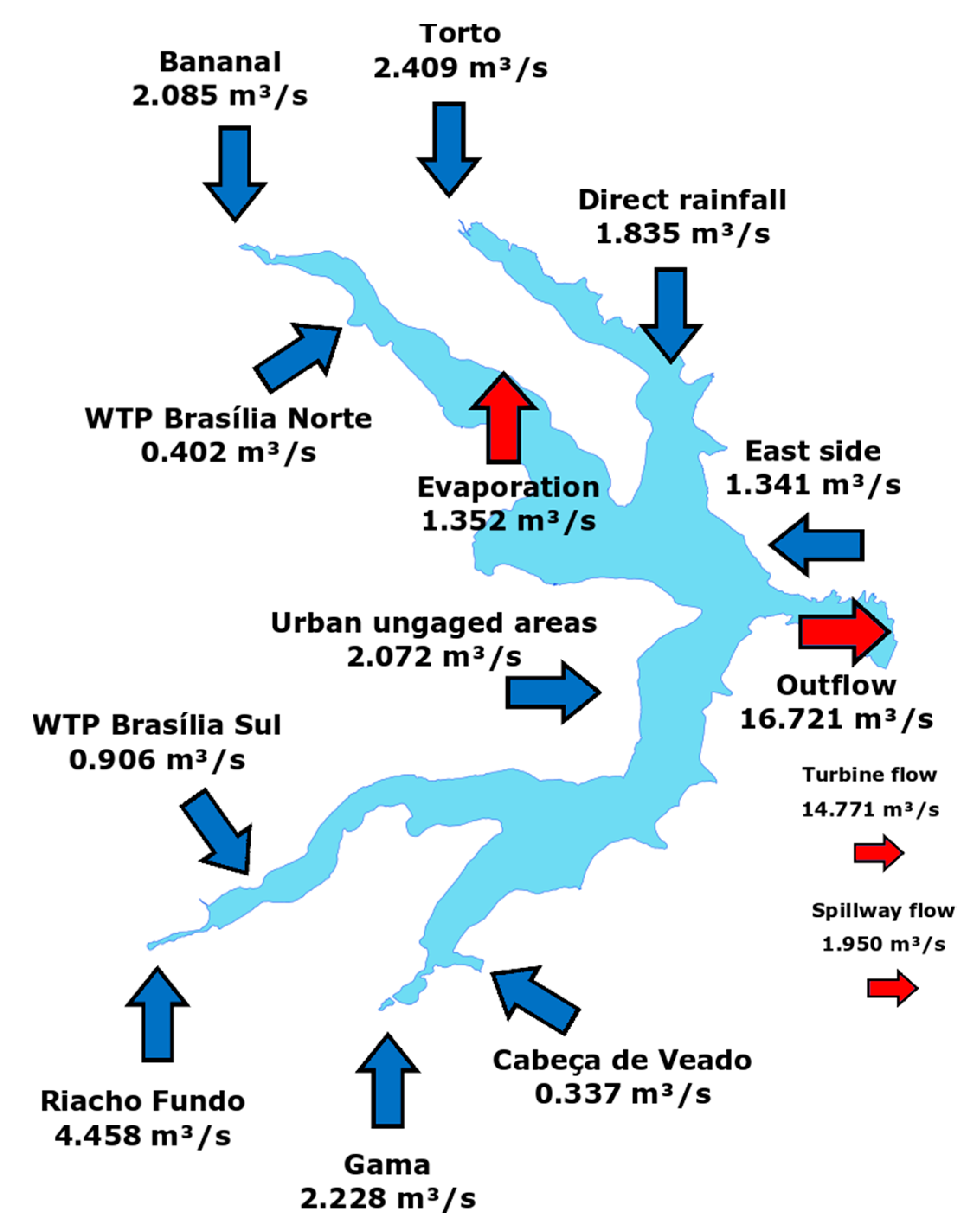
Approximately 80% of the water inflow to Paranoá Lake is gauged, either by the outflow from the sub-basins or indirectly by rainfall throughout the basin. The ungauged areas correspond to about 20%. The result shown in Table 9 is presented graphically in Figure 17. The blue arrows represent inlet flows into Paranoá Lake, while the red arrows represent system water losses.

As noted in Figure 17, the largest average long-term contribution is the Riacho Fundo sub-basin with approximately 4.5 m³/s, representing almost 25% of the contribution to Paranoá Lake alone.

The Bananal and Gama sub-basins have very close contributions; this is due to the similarity between their contribution areas (Bananal = 125.76 km², Gama = 136.55 km²), as well as the presence of large areas of preserved native vegetation. The Torto sub-basin also fits into this profile, however, they have two fundamental differences, the first is that it has a larger area of about 233.4 km² and the second is that it is one of the sub-basins that are a source of public supply in the DF, which justifies long-term inflows close to that observed in Gama and Bananal.

As for the contributions of the WTPs, together they reach a long-term flow close to the evaporated flow in the water surface, around 1.3 m³/s.

The unmonitored areas, urban and east side, had long-term flows estimated at 2.072 m³/s and 1.341 m³/s, respectively, which represents an important portion for maintaining the volume of Paranoá Lake.

Finally, the total loss of water from the Paranoá Lake is given by the sum of the dam outflow and the evaporated flow, which together correspond to 18.073 m³/s. The dam outflow can also be divided into turbine flow with 14.771 m³/s and spillway flow with 1.950 m³/s.

5. Discussion

Despite the performance of some studies on sub-basins affluent to Lake Paranoá [17], the elaboration of a long-term study, which considers the entire area affluent to Lake Paranoá, with all its contribution area and its physical and meteorological characteristics, still has not been accomplished. In this context, we conducted a study that integrated, through the focus of mathematical modeling, physical, meteorological, and hydrological data for more than 30 years. Using the SWAT model, we approached the characteristics of the sub-basins affluent to Lake Paranoá and reproduced their behavior efficiently and satisfactorily over the last three decades. Our approach considered that the analysis should be carried out in three different periods considering the availability of data. Then, we considered the first period used for the calibration of the model from 1982 to 2000, and then the validation was carried out in two stages, with the first performed with data from 2001 to 2010 and the second from 2011 to 2017. It is an approach that differs slightly from those traditionally adopted that consider only two periods, such as calibration and verification. However, the division in these periods considers a dynamics of the use of the basin that occurred in these periods, with the first period (calibration—1982 to 2000) being a time marked by intense occupation of the basin, the second period (first verification—2001 to 2010) being a transition period between stabilization, and finally the third period (second verification—2011 to 2017) being a time when the achievement of stability is observed.

In these three periods (1982–2000, 2001–2010, 2011–2017), we sought to evaluate the performance of the model in the representation of the hydrological processes of the sub-basins affluent to Paranoá Lake. We carried out the calibration using NSE and PBIAS as evaluation metrics [45], and SUFI-2 as a method of parameter optimization, considering its efficiency for optimization of distributed models [24,26]. With this approach, the model performed well in the representation of the basins. The parameter optimization and the uncertainty analysis were executed within the SWAT-Cup, wherein the SUFI-2 algorithm was applied. We observed that after three SUFFI-2 iterations, with 1900 runs in each iteration, the modelling reached good performance, shown in this work. The uncertainty analysis regarding the parameters was conducted with the evaluation of the P-factor and R-factor values at the end of each iteration to have P-factor values close to 0 and R-factor values below 1.5, as well as reducing the 95PPU range [24,25,26,40,41,42,43].

We plotted the parameter values and the respective NSE value for the three SUFI-2 iterations performed in the Swat-Cup to observe the relationship parameter objective function, with a substantial improvement being achieved in the modeling process, showing the effectiveness of the use of SWAT in the sub-basins affluent to Lake Paranoá. We found that the parameters selected as the most sensitive in each sub-basin are reported in several studies in other Brazilian basins [18,27,28,29,46], but also different places around the world [1,10,22,25,26,42].

For the study of the water balance of Paranoá Lake, the contribution of the areas of direct drainage to the lake needed to be estimated because they represent a significant part of the contributing area. This was done on the basis of the modeled sub-basins, using as criteria the fact that the directly contributing area has similar behavior of the modeled areas with similar characteristics [6] such as slopes and land use/land cover. This approach was used because it would not be possible to calibrate/validate the modelling.

Extrapolating information from gauged basins to ungauged areas is always a challenge in hydrology. When a basin dataset is lacking, neighboring basins with similar characteristics can be used as a parameter for the estimates. The similarity between gauged and ungauged basins can be established from a comparison of physical factors [6]. An alternative is to integrate various pieces of information about reservoirs in SWAT in order to model the basin–lake set, however, as discussed previously, there is a limitation of the model in receiving a dynamic reservoir dataset, i.e., a series of operation data of the reservoirs (turbine and spillage flows), and it is allows only the insertion of historical monthly flows into the model. This limitation may directly affect the water balance due to factors such as extreme weather events, the size of the reservoir, and the dynamics of flow outlet operation, and thus it can introduce difficulties for reservoir management decision making. For this reason, we applied the SWAT model to all gauged sub-basins and then carried out the water balance, considering the dynamics of the reservoir’s operation, as we understand that this is the most feasible way to analyze basins with this level of complexity.

6. Conclusions

This paper carried out a study to determine the water balance of Paranoá Lake. The SWAT model was used in the hydrological study of each affluent sub-basin. After the calibration and validation steps of the gauged sub-basins, we estimated the contributing flows from ungauged areas.

It was the first time that the extensive monitored tributary flow database (35 years) was used in the modeling of PLB. The study was also a pioneer in using hydrological modeling data in the representation of affluent flows from ungauged affluent basins. The results generated from the hydrological modeling showed good performance of the SWAT model, even in the Riacho Fundo sub-basin, which has a high degree of urbanization, confirming that the model can also be used for the estimation of hydrological processes for urban basins.

The results generated by the SWAT model showed the importance of the base flow for the maintenance of the flows in each sub-basin and consequently for Paranoá Lake. Thus, anthropogenic interventions in the basin that increase impermeabilization, as has been occurring in recent years, should be avoided, as this will dramatically change the hydrological processes, and it will certainly affect the flow regime of each sub-basin and, consequently, Paranoá Lake.

We believe that the improvement achieved in the simulation of the contributing basins to the lake using the SWAT model will improve the water management of the lake and its hydrological basin, a very important contribution considering the growing importance of the lake as a water supply source. One important modelling aspect observed is the flow discharge from reservoirs, as occurs with the sub-basins of Torto and Cabeça de Veado. In the current SWAT version, data input is based on long-term monthly averages and not on time series data; thus, even if continuous flow monitored data is available, these data must be converted to historical averages and inserted into the model. This aspect of the model certainly has an impact on the efficiency of the model in representing such basins since the long-term monthly average may not be representative in years of extreme events, notably in lakes such as the Paranoa, with a small range of permitted stage variation (1 m).

The Paranoá Lake water balance was performed on the basis of the continuity equation integrating the results generated for each area affluent to the lake. This approach proved to be effective in both diagnosing the hydrological characteristics of each sub-basin and calculating the long-term water balance in Paranoá Lake, as well as allowing future water management studies by performing simulations with different occupation scenarios, which is very dynamic due to the urban expansion into the PLB.

Analysis over time identified the Riacho Fundo sub-basin as the largest contribution to Paranoá Lake, representing about 24% of the total flow that reaches into the lake. From the analyzed period, the years with the lowest water balance were the years 1986, 1996, 1999, and 2003, which are associated with smaller annual rainfall. The determination of the inlet water volumes into Paranoá Lake is very important in the management of the lake, both in terms of water balance aspects for the allocation of each service and in terms of aspects of water quality management. Considering the problems in evaluating the lake surface water outflows and the large population growth and consequent land use change in the basin, we believe that hydrological modeling is essential for water management scenarios.

On the basis of the results obtained in this study, we were able to verify that this type of analysis—one that is associated with the hydrological modeling of the affluent basins as a support for understanding the effect of possible changes that may occur in the PLB and the effects of such changes in the water balance of the lake, a system subjected to multiple uses with already severe restrictions on water level variation—can be used in the Brazilian Federal District for water source management improvement purposes, as well as in the study of other urban lake basins.