Using Stable Isotopes to Determine the Water Balance of Utah Lake (Utah, USA)

Abstract

To investigate the hydrology of Utah Lake, we analyzed the hydrogen (δ²H) and oxygen (δ¹⁸O) stable isotope composition of water samples collected from the various components of its system. The average δ²H and δ¹⁸O values of the inlets are similar to the average values of groundwater, which in turn has a composition that is similar to winter precipitation. This suggests that snowmelt-fed groundwater is the main source of Utah Valley river waters. In addition, samples from the inlets plot close to the local meteoric water line, suggesting that no significant evaporation is occurring in these rivers. In contrast, the lake and its outlet have higher average δ-values than the inlets and plot along evaporation lines, suggesting the occurrence of significant evaporation. Isotope data also indicate that the lake is poorly mixed horizontally, but well mixed vertically. Calculations based on mass balance equations provide estimates for the percentage of input water lost by evaporation (~47%), for the residence time of water in the lake (~0.5 years), and for the volume of groundwater inflow (~700 million m³) during the period April to November. The short water residence time and the high percentage of total inflow coming from groundwater might suggest that the lake is more susceptible to groundwater pollution than to surface water pollution.

1. Introduction

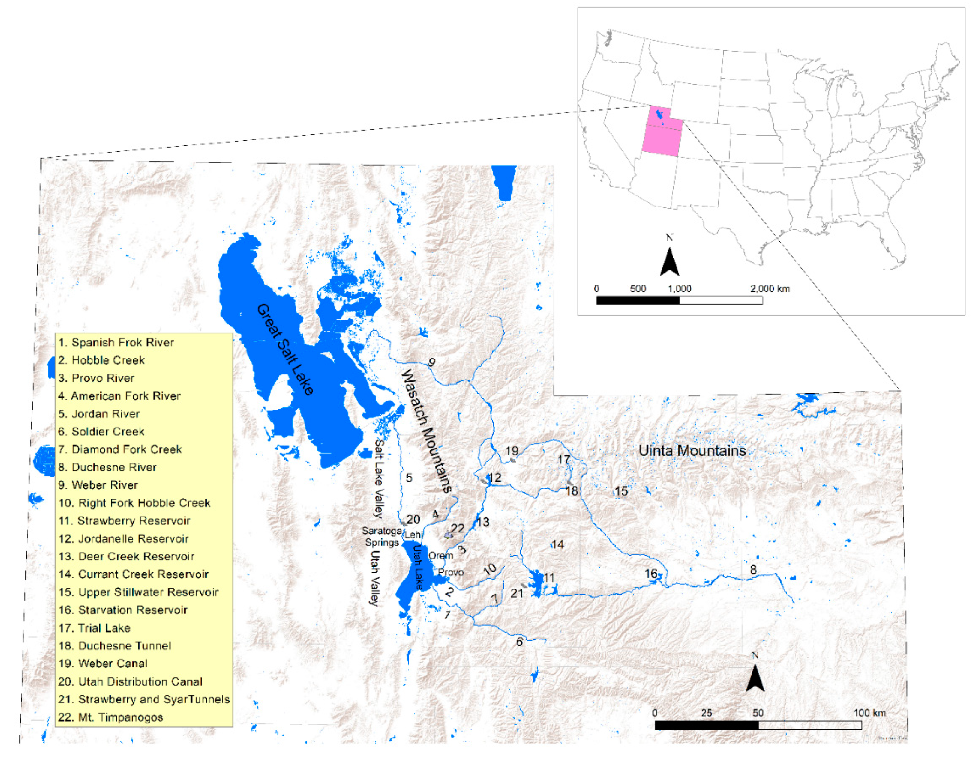
Utah Lake is, by surface area, the third largest natural freshwater lake in the western US. It is in north-central Utah (in Utah Valley and Utah County), near the cities of Provo and Orem (Figure 1). When at its highest level, the lake is ~39 km long and ~21 km wide and has a surface area of ~390 km² [1]. It is a very shallow lake (its maximum and average depths are ~6 m and ~3 m, respectively) having eutrophic, turbid, slightly saline and alkaline water [2]. The lake is a remnant of the much larger Lake Bonneville, from which it formed ~8000 years ago [2]. Its floor is composed almost entirely of alluvium while the mountains east and west of the lake are made of bedrock dominated by carbonate lithologies [2]. The principal constituent of its sediment is calcium carbonate, which precipitates by evaporative concentration and by the activity of algae and microorganisms and accumulates at rates of 1–2 mm·year⁻¹ [2,3]. The lake is a component of the Central Utah Water Project [4], a federal project designed to deliver water for irrigation, power generation, recreation, and municipal and industrial use. The project has a complex system of reservoirs, tunnels, canals, and pipelines. The water flow entering and exiting the lake is adjusted based on the irrigation and agricultural needs and the level of the lake is kept at an approximately constant level (the “compromise water level”, 1368.35 m a.s.l.; [5]). The most important inlets for the lake are the Spanish Fork River, the Provo River, Hobble Creek, and the American Fork River. The lake has only one outlet, the Jordan River, which flows north into the Great Salt Lake (Figure 1). Exposed and submerged springs and seeps occur along the eastern and northern margins and near the deepest point of the lake [2,6,7]. These springs appear to be hydraulically connected to shallow groundwater systems [6].

With respect to the inlets, the Spanish Fork and Provo rivers represent the biggest stream inflow to the lake. Their flow is highly regulated through the structures of the Central Utah Water Project. The Spanish Fork River has a long-term (1990–2019) median discharge of 6.63 m³·s⁻¹. It forms at the confluence of Soldier Creek and Thistle Creek in the Wasatch Mountains and flows for 32 km. The river imports water from Strawberry Reservoir through the Syar and Strawberry tunnels and from the tributary of Diamond Fork Creek. The Provo River (median discharge = 3.87 m³·s⁻¹) provides drinking water for over half of Utah’s population [8]. It forms from Trial Lake, a small reservoir in the Uinta Mountains, and flows for 100 km. The river receives water diverted from the Duchesne and Weber rivers through the Duchesne Tunnel and Weber Canal before draining first into the Jordanelle and then into the Deer Creek reservoirs. Hobble Creek and the American Fork River represent minor inflows to the lake. Hobble Creek (median discharge = 0.78 m³·s⁻¹) forms at the confluence of the Left Fork and Right Fork Hobble Creek in the Wasatch Mountains and flows for 17 km. The American Fork River (median discharge = 1.14 m³·s⁻¹) forms on Mount Timpanogos (Wasatch Mountains) and flows for 56 km.

The Jordan River (median discharge = 3.53 m³·s⁻¹) flows for 82 km from the north end of the lake to the Great Salt Lake through the Utah and Salt Lake valleys. Pumps located at its headwaters control its flow. Two dams and several canals divert water to surrounding areas for irrigation purposes. The water diverted through the Utah Lake Distribution Canal eventually enters back into the lake.

In recent years, Utah Lake has faced serious issues of pollution and harmful algal blooms [9]. In addition, the state of Utah is expected to face water quantity and quality challenges as its population increases and global and regional climates change [10,11,12]. As a result, Utah Lake represents a crucial freshwater resource for the ~500,000 people living in Utah Valley. However, only a handful of studies have been performed on the hydrology of the lake [1,3,7,13]. In addition, these studies are flawed, as they lack a description of the model used [1] or rely on the questionable assumption of a negligible rate of groundwater outflow [3]. Therefore, the main purpose of this study is to investigate the hydrology of the lake via oxygen and hydrogen stable isotope analysis of water samples collected from the different components of the Utah Lake system. Several studies have successfully employed oxygen and hydrogen stable isotopes in lake water. For instance, isotopes have been used to investigate lake water balance and water residence time [14,15,16,17], direction of water flow [18], interaction of lake water with surrounding groundwater [19,20,21,22], and lake stratification [23,24]. In this context, the specific objectives of this study were: (i) to characterize the isotopic composition of the most important hydrological components of the lake system (i.e., meteoric precipitation, the inlets, the Jordan River, groundwater, and the lake); (ii) to provide general information about lake mixing and stratification; and (iii) to estimate some hydrological parameters for the lake (i.e., the fraction of input water that is lost by evaporation, the water residence time, and the rate of groundwater inflow). These parameters are important because they are correlated with various chemical stressors [14,25,26]. The results of this study will provide information on the factors controlling lake water quality, quantity, and biological conditions, therefore helping state agencies in the sustainable management of this important resource. In addition, the data presented here can also help future studies in the interpretation of the stable isotope records of paleoclimate and paleohydrology derived from the lake sediments.

2. Materials and Methods

2.1. Sample Collection and Isotope Analyses

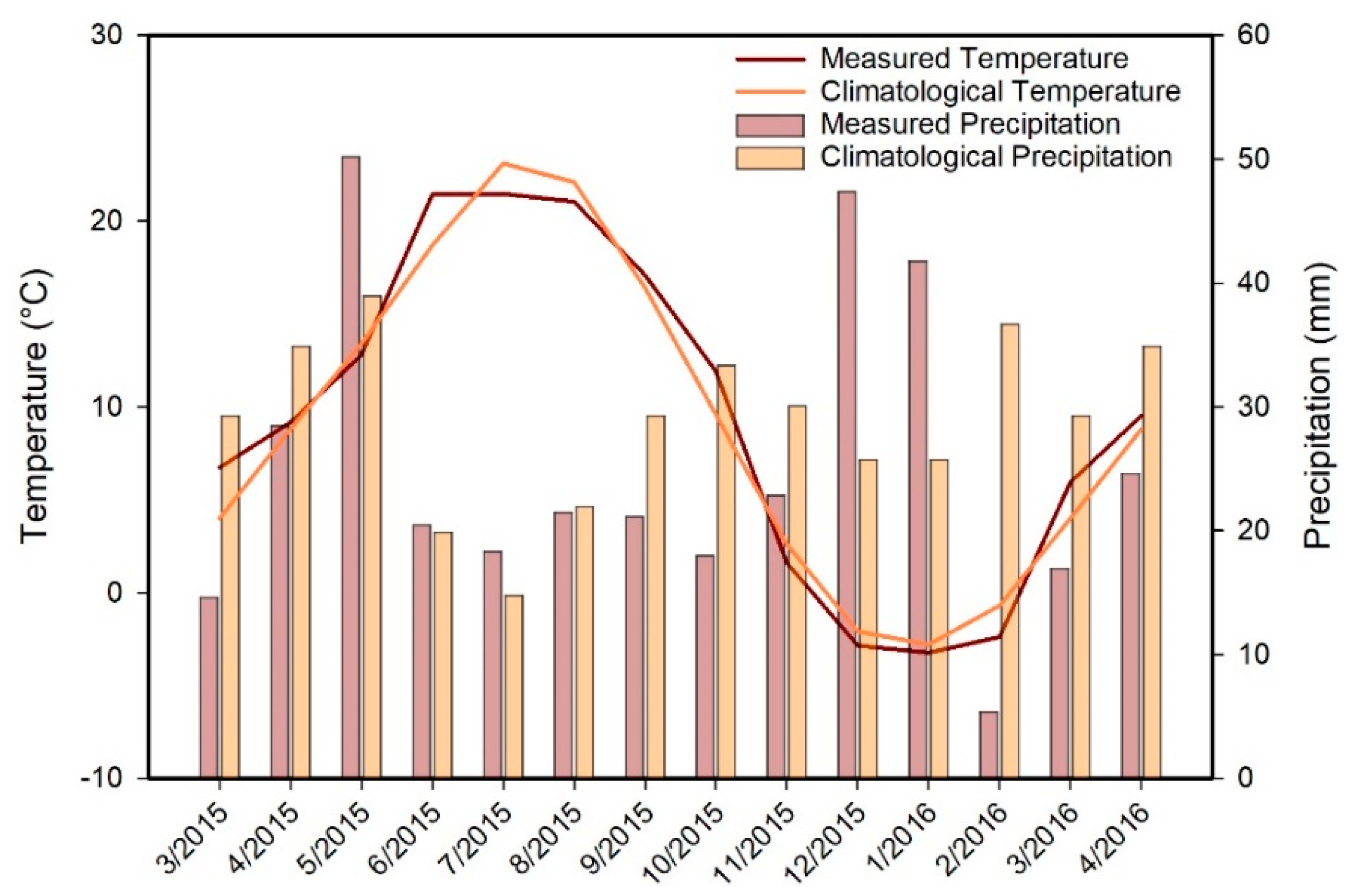
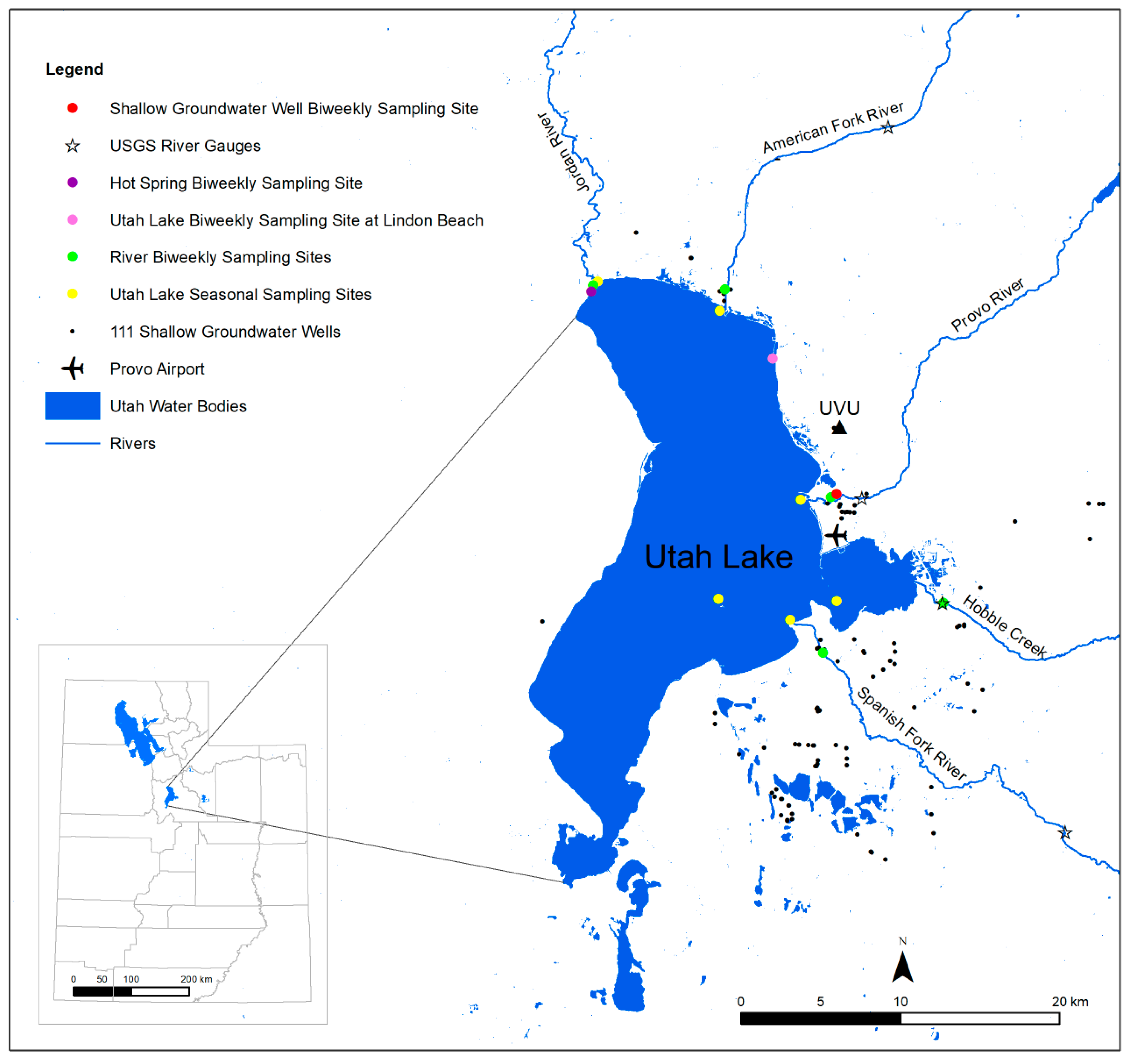
We conducted most of the work for this study between March 2015 and April 2016. Temperature and precipitation during the study period were generally similar to climatology (Figure 2), suggesting that our results can be representative of any meteorologically average year. Between March 2015 and March 2016, we collected biweekly water samples from the inlets, the Jordan River, a shallow groundwater well (well 55–3259; depth = 38.7 m), Utah Lake at Lindon Beach, and from a hot spring in Saratoga Springs (Figure 3). The water in this hot spring has a temperature of 40 °C. As a result, assuming a geothermal gradient of ~28 °C·km⁻¹, the difference between the temperature of the hot spring and the mean annual air temperature indicates that the hot spring water must flow from a depth of at least ~1 km. In addition to these biweekly samples, we collected seasonal samples in April, July, and November 2015 at five locations spread over the entire lake from depths of ~10 and ~40 cm (Figure 3). During the same seasonal sampling campaigns, we collected additional lake samples along a depth profile at 0.5-m increments with a Geotech Geopump peristaltic pump. In addition to the lake, river, well water, and hot springs samples, we collected samples of cumulative monthly meteoric precipitation at the campus of Utah Valley University (UVU; Figure 3) from April 2015 to April 2016. In order to prevent the evaporation of meteoric water, we employed a special collector available from the company Palmex [27]. Finally, we collected samples from 111 Utah Valley shallow groundwater wells (all less than 10 m deep) in June 2014 and in June and July 2015 (Figure 3). Except for the well water, we filtered all the samples in the field with Cameo 0.22-μm nylon filters and placed them in 30 mL glass vials. To prevent evaporation, we filled the vials to the top (i.e., no headspace), and we capped and sealed them with a layer of Parafilm. Finally, we stored the samples in a refrigerator with a temperature of 4 °C before the analyses.

We obtained discharge data for the Spanish Fork River (gauging station 10150500), Hobble Creek (gauging station 10153100), Provo River (gauging station 10163000), and American Fork River (gauging station 10164500) from gauges of the US Geological Survey (Figure 3) [29]. We obtained climate data recorded at 20 min intervals from the National Weather Service station of the Provo Airport [30], which is located on the lake’s eastern shore (Figure 3).

We analyzed all the water samples for their hydrogen and oxygen stable isotope composition. All isotope compositions are expressed with the conventional δ notation in parts per thousand or permil (‰) according to the following equation:

$$\delta =\left(\frac{R_{sa}}{R_{st}}-1\right)·1000 (‰)$$

(1)

where δ is the δ²H or δ¹⁸O of the sample, R_sa is the isotope ratio (²H/¹H or ¹⁸O/¹⁶O) in the sample, and R_st is the same isotope ratio in a standard. All compositions are reported relative to the SMOW (Standard Mean Ocean Water) standard. The samples from the 111 shallow groundwater wells were analyzed at the University of Utah using a Picarro (model L2130i) Liquid Water Isotope Analyzer. We analyzed all the other samples with a Los Gatos Research (LGR) Liquid Water Isotope Analyzer (model 912-0008) housed in the Earth Science Geochemistry Lab of UVU. We ran each sample in triplicates with six injections performed on each replicate. We discarded the first two injections due to possible memory effects and averaged the last four injections to determine the δ²H and δ¹⁸O values of each sample. We normalized the data with the block standardization method using the standards LGR 1c (δ²H = −154.0 ± 0.5‰; δ¹⁸O = −19.49 ± 0.15‰) and LGR 4c (δ²H = −51.6 ± 0.5‰; δ¹⁸O = −7.94 ± 0.15‰). We used the standard LGR 3c (δ²H = −97.3 ± 0.5‰; δ¹⁸O = −13.39 ± 0.15‰) as an internal quality control. Based on replicate measurements of this internal standard, the precision (i.e., ±1 sd) of these measurements is better than 1‰ (δ²H) and 0.2‰ (δ¹⁸O).

2.2. GIS Analyses

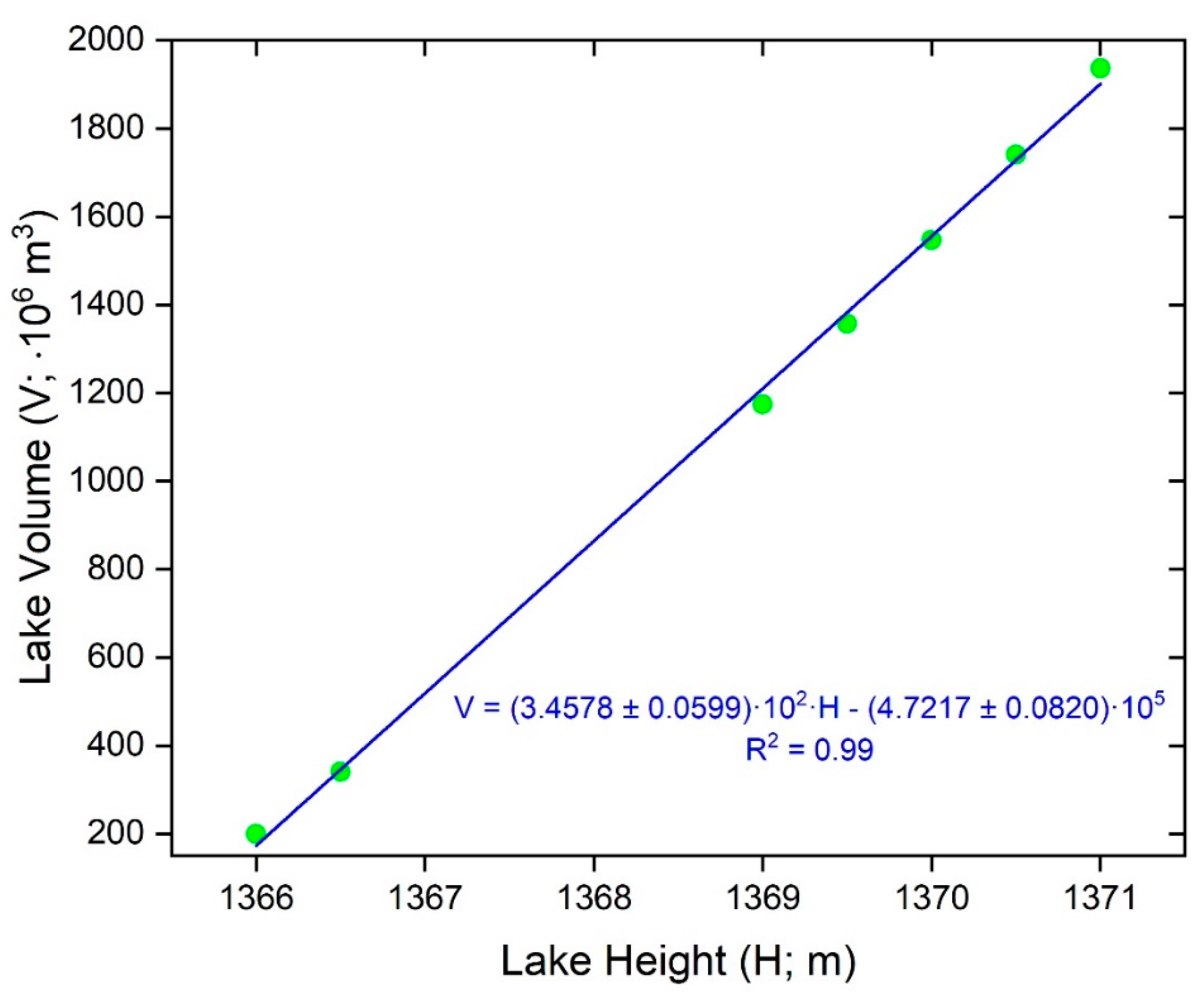
We derived an equation relating lake volume with lake height using the software ArcGIS 10.5. We acquired a bathymetric map of Utah Lake from the Bureau of Reclamation (sounding below winter ice) [31] and shoreline LiDAR data from Open Topography [32]. We operated both datasets within the NAVD88 Vertical Datum and NAD83 UTM zone 12 coordinate systems. We degraded the LiDAR dataset to a 30 m grid cell area, smoothing the data significantly but preserving major shoreline features. From the degraded 30 m dataset, we created 0.1 m interval shoreline elevation contour lines extending between 1366 and 1372 m a.s.l. These elevation contours were then merged with the bathymetric contours to produce a contour data set from the lake bottom to 1372 m a.s.l. (an average maximum height for the lake). Finally, we used the topo to raster tool (3D analyst in the toolbox) to convert the topolines to a digital elevation model (DEM) grid with a 5 × 5 m resolution. We then generated single value DEM’s across the entire lake surface for the following lake contour areas: 1366.0 m, 1366.5 m, 1369.0 m, 1369.5 m, 1370.0 m, 1370.5 m, and 1371.0 m. For each of these areas, we subtracted the single value DEM from the DEM of the lake bathymetry, obtaining a DEM of lake height. For each of the lake height DEM’s, we multiplied each grid cell by its area (25 m²) to produce a lake volume grid, which we used to sum the total lake volume for each lake height. We then plotted lake volume vs. lake height obtaining the following linear relationship (Figure 4):

$$V=\left(3.4578\pm 0.0599\right)·{10}^2·H-\left(4.7217\pm 0.0820\right)·{10}^5$$

(2)

where V is the volume of the lake in millions of m³ and H is the height of the surface of the lake in m.

We modeled the spatial distribution in the δ²H and δ¹⁸O values of the lake using the inverse distance weighted (IDW) interpolation spatial analysis method. After the interpolation, we used the Extract by Mask tool in ArcToolbox to display the spatial variability in the δ-values of Utah Lake.

2.3. Calculation of Utah Lake Hydrological Parameters

We used mass balance equations originally developed by Dincer [33] and then modified by Gibson et al. [34] in order to calculate the hydrological parameters of the lake. In a throughflow lake such as Utah Lake, the change in volume over time must be equal to the sum of the inflows minus the sum of the outflows:

$$\frac{dV}{dt}=G_i+P+S_i-G_o-E-S_o$$

(3)

where dV/dt is the change in lake volume over time, G_i is the groundwater inflow, P is the meteoric precipitation falling on the lake surface, S_i is the surface water inflow, G_o is the groundwater outflow, E is the evaporation, and S_o is the surface water outflow. Each term in the equation above can be expressed as a rate (with dimensions of [L³/T] or equivalently [L/T] if normalized to the lake surface), as a volume ([L³]), or mass ([M]). The equation above can be combined with an isotopic mass balance equation in which each term is multiplied by its isotopic composition:

$$\frac{dV·{\delta }_L}{dt}=G_i·{\delta }_{Gi}+P·{\delta }_P+S_i·{\delta }_{Si}-G_o·{\delta }_{Go}-E·{\delta }_E-S_o·{\delta }_{So}$$

(4)

where the δs refer to the δ²H or δ¹⁸O of the lake (δ_L), of the groundwater inflow (δ_Gi) and outflow (δ_Go), of meteoric precipitation (δ_P), of the surface water inflow (δ_Si) and outflow (δ_So), and of the evaporative flux (δ_E). Assuming hydrologic steady state (i.e., dV/dt = 0) and following the approach of Gibson et al. [34], these equations can be solved to find the dimensionless throughflow index, E/I:

$$\frac{E}{I}=\frac{\left({\delta }_L-{\delta }_I\right)}{m·\left({\delta }^{*}-{\delta }_L\right)}$$

(5)

where E/I is the fraction of total (i.e., both surface and subsurface) inflow that is lost by evaporation, δ_L is the steady state δ²H or δ¹⁸O value of the lake and δ_I is the δ²H or δ¹⁸O value of the input water. In addition, m is given by:

$$m=\frac{\left(h-{10}^{-3}·\left({\epsilon }_K+\frac{{\epsilon }^{+}}{{\alpha }^{+}}\right)\right)}{\left(1-h+{10}^{-3}·{\epsilon }_K\right)}$$

(6)

where h is the atmospheric relative humidity (entered as a fraction), ε_K and ε⁺ are, respectively, the kinetic and equilibrium isotopic separations (given in ‰) between liquid water and water vapor (i.e., δ²H_water-δ²H_vapor or δ¹⁸O_water-δ¹⁸O_wapor), and α⁺ are the equilibrium fractionation factors between liquid water and water vapor $\left(\mathrm{i}.\mathrm{e}.,\frac{{\left(\frac{2H}{1H}\right)}_{water}}{{\left(\frac{2H}{1H}\right)}_{vapor}}\mathrm{or} \frac{{\left(\frac{18O}{16O}\right)}_{water}}{{\left(\frac{18O}{16O}\right)}_{vapor}}\right)$. With respect to ε⁺ and α⁺, they are related by:

$${\epsilon }^{+}=\left({\alpha }^{+}-1\right)·{10}^3‰$$

(7)

and ε_K is given by:

$${\epsilon }_K=\theta ·C_K·\left(1-h\right)‰$$

(8)

where θ is a transport resistance parameter commonly assumed to be equal to 1 and C_K is a kinetic constant commonly assumed to be 14.2‰ for oxygen isotopes and 12.5‰ for hydrogen isotopes.

Finally, δ* is the limiting δ²H or δ¹⁸O value of the lake and is given by:

$${\delta }^{*}=\frac{\left(h·{\delta }_A+{\epsilon }_K+\frac{{\epsilon }^{+}}{{\alpha }^{+}}\right)}{\left[h-{10}^{-3}·\left({\epsilon }_K+\frac{{\epsilon }^{+}}{{\alpha }^{+}}\right)\right]}‰$$

(9)

where δ_A is the δ²H or δ¹⁸O value of atmospheric water vapor. The fractionation factors α⁺ are temperature dependent and can be calculated using the equations of Horita and Wesolowski [35]. For hydrogen isotopes, the equation is given by:

$${\alpha }^{+}=exp\left[1158.8·\left(\frac{{\left(273.15+T\right)}^3}{{10}^{12}}\right)-1620.1·\left(\frac{{\left(273.15+T\right)}^2}{{10}^9}\right)+794.84·\left(\frac{\left(273.15+T\right)}{{10}^6}\right)-\frac{161.04}{{10}^3}+\frac{2999200}{{\left(273.15+T\right)}^3}\right]$$

(10)

whereas for oxygen isotopes the equation is given by:

$${\alpha }^{+}=exp\left[-\frac{7.685}{{10}^3}+\frac{6.7123}{\left(273.15+T\right)}-\frac{1666.4}{{\left(273.15+T\right)}^2}+\frac{350410}{{\left(273.15+T\right)}^3}\right]$$

(11)

At hydrologic steady state, the residence time of water in the lake is given by:

$$\tau =\frac{V}{I or O}$$

(12)

where τ is the residence time, V the volume of the lake, I the total inflow and O the total outflow (by definition, at hydrologic steady state I = O). Given E/I, it is then possible to calculate the residence time of the water in the lake using the following equation:

$$\tau =\frac{E}{I}·\frac{V}{E}$$

(13)

To estimate E, we used the simplified version of the Penman equation developed by Valiantzas [36]:

$$E_r=0.047·R_S·\sqrt{T+9.5}-2.4·{\left(\frac{R_S}{R_A}\right)}^2+0.09·\left(T+20\right)·\left(1-h\right)$$

(14)

where E_r is the evaporation rate in mm·day⁻¹, R_S is the solar radiation in MJ·m⁻²·day⁻¹, T is the temperature in °C, and h the atmospheric relative humidity (entered as a fraction). The extraterrestrial radiation R_A (in MJ·m⁻²·day⁻¹) can be calculated from the following equation:

$$R_A=3·N·\sin \left(0.131·N-0.95\mathsf{\Phi }\right)$$

(15)

where Φ is the latitude of the site in radians (positive for the northern hemisphere and negative for the southern hemisphere) and N is given by:

$$N=4· \mathsf{\Phi }·\sin \left(0.53·i-1.65\right)+12$$

(16)

where i is the rank of the month (i.e., January = 1, February = 2, etc.).

The most difficult term to estimate in a water balance equation is the groundwater inflow. Assuming that the lake is at hydrologic steady state and well-mixed (i.e., δ_Go = δ_So = δ_L), we estimated it using the equation provided by Krabbenhoft et al. [20]:

$$G_i=\frac{\mathrm{P}\left({\delta }_L-{\delta }_P\right)+S_i\left({\delta }_L-{\delta }_{Si}\right)+E\left({\delta }_E-{\delta }_L\right)}{\left({\delta }_{Gi}-{\delta }_L\right)}$$

(17)

With respect to δ_E (which is the δ²H or δ¹⁸O value of the evaporative flux), we calculated it using the Craig and Gordon equation [37]:

$${\delta }_E=\frac{\left(\frac{{\delta }_L-{\epsilon }^{+}}{{\alpha }^{+}}-h·{\delta }_A-{\epsilon }_K\right)}{\left(1-h+{10}^{-3}·{\epsilon }_K\right)}‰$$

(18)

3. Results and Discussion

Tables S1–S5 report the entire dataset of the study.

Table 1. Summary descriptive statistics for the δ-values of meteoric precipitation and of the biweekly samples. X_GW is the average fraction of groundwater vs. meteoric precipitation present in the stream flow of each inlet. Latitude and longitude are referenced to the WGS (World Geodetic System) 84 datum.

	Latitude (°N)	Longitude (°W)	n samples	Avg. δ2H (‰)	SD	Range	Avg. δ18O (‰)	SD	Range	XGW
Meteoric Precipitation	40.2778	111.7147	12	−90.2	27.9	102.9	−12.73	3.06	11.06
Well Water and Hot Spring
Well Water	40.24	111.7175	27	−126.2	0.7	4	−17.08	0.23	1.19
Saratoga Springs Hot Spring	40.3531	111.9	25	−125.6	0.5	2.7	−16.66	0.16	0.76
Rivers
Spanish Fork River	40.1503	111.7264	26	−112.3	2.9	10.7	−14.69	0.54	2.4	0.49
Hobble Creek	40.1789	111.6381	27	−114.4	8.4	19.3	−15.17	1.58	4.08	0.62
Provo River	40.2381	111.7217	26	−118.8	0.9	3.3	−16.07	0.32	1.4	0.87
American Fork River	40.355	111.8014	26	−119.9	1.4	4.3	−16.54	0.42	1.41	0.98
Jordan River	40.3567	111.8989	26	−90.4	14	60	−10.75	2.66	10.94
Utah Lake	40.3161	111.7656	26	−76	10.2	37.7	−8.32	1.87	7.05

reports summary descriptive statistics of the δ-values for the monthly samples of meteoric precipitation and for all the biweekly samples (i.e., the samples from the shallow groundwater well, the hot spring, the inlets, the Jordan River, and Utah Lake). Figure 5 shows plots of the δ²H and δ¹⁸O values for all the biweekly samples vs. time and Figure 6 shows a plot of the δ²H vs. δ¹⁸O values for all the biweekly samples, for the monthly samples of meteoric precipitation, and for the samples of the 111 shallow groundwater wells. With respect to the seasonal samples, Figure 7 shows depth profiles of lake water δ²H and δ¹⁸O values and Figure 8 shows spatial patterns in the δ²H and δ¹⁸O values of the samples collected throughout the lake.

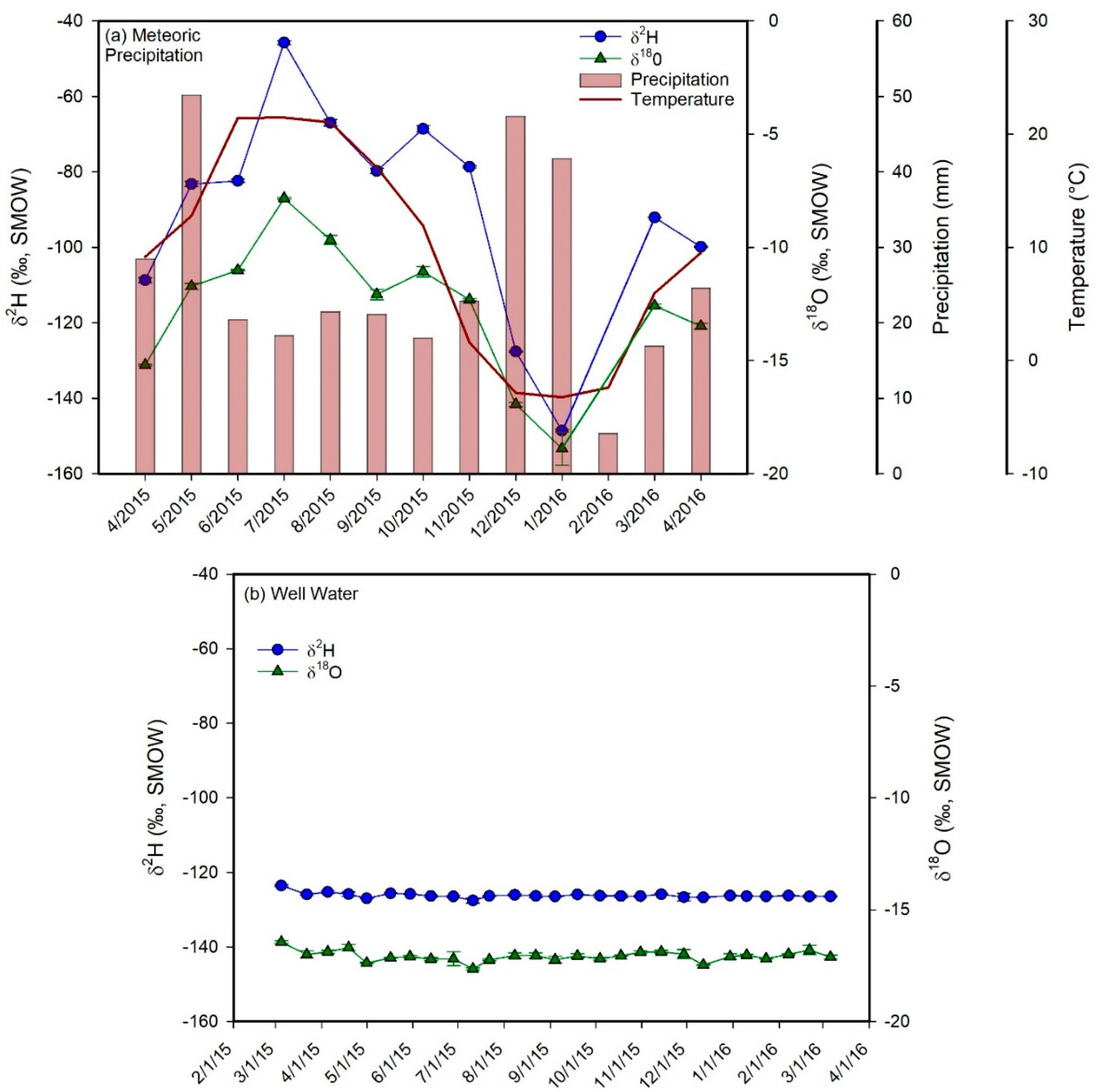
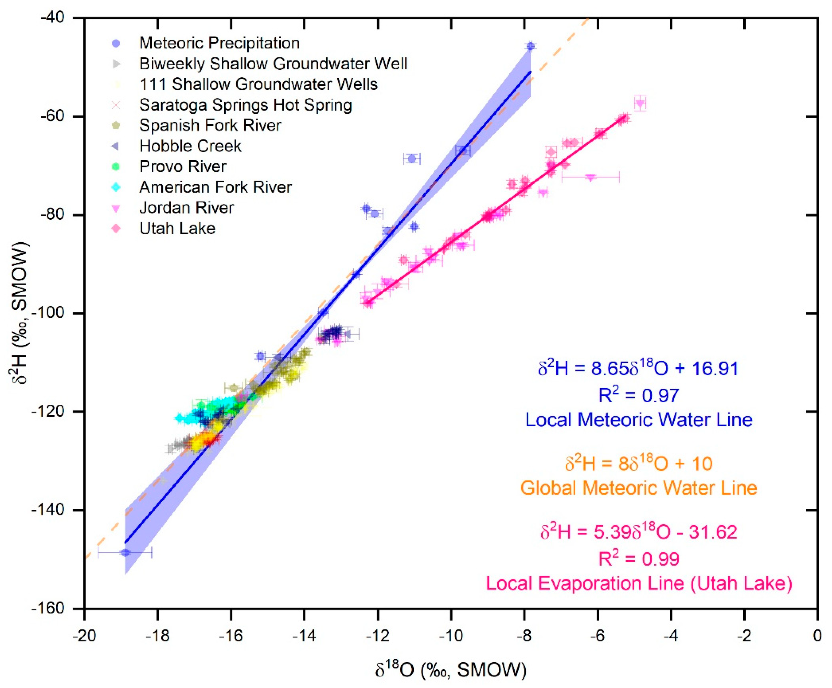
Data for meteoric precipitation are included in the Global Network of Isotopes in Precipitation [38]. We eliminated from the data analysis and interpretation, the δ-values for February 2016 because the sample showed evidence of evaporation. With respect to δ²H, values for meteoric precipitation range from −148.6‰ to −45.7‰ and average −90.2 ± 27.9‰ (all averages are reported ±1 sd.). With respect to δ¹⁸O, values range from −18.89‰ to −7.83‰ and average −12.73 ± 3.06‰. Both δ²H and δ¹⁸O values show a marked seasonality with highest values in July and lowest values in January (Figure 5a). In a plot of δ²H vs. δ¹⁸O values, the samples of meteoric precipitation define a local meteoric water line (LMWL; Figure 6) that has the following equation:

$$\delta 2H=\left(8.65\pm 0.48\right)·\delta 18O+\left(16.91\pm 6.02\right)$$

(19)

This line is very similar to the global meteoric water line reported in [39]:

$$\delta 2H=8·\delta 18O+10$$

(20)

The composition of meteoric precipitation can be weighted by amount by using this formula:

$${\delta }_P=\frac{{{\displaystyle \sum }}_{i=1}^{i=12}{\delta }_{P\left(i\right)}{P}_i}{{{\displaystyle \sum }}_{i=1}^{i=12}{P}_i}$$

(21)

where δ_P(i) represents the δ²H or δ¹⁸O value of meteoric precipitation integrated over month i and P_i is the amount of precipitation fallen during month i. When weighted by amount using this formula, annual average δ²H and δ¹⁸O values of meteoric precipitation are −97.1‰ and −13.59‰, respectively.

The δ²H and δ¹⁸O values of the biweekly well water samples are remarkably constant over time and average −126.2 ± 0.7‰ and −17.08 ± 0.24‰, respectively (Figure 5b). Samples from the 111 shallow wells also show a low spatial variability, and average −123.0 ± 5.0‰ in δ²H and −16.33 ± 0.87‰ in δ¹⁸O. The values for all these groundwater samples are similar to those of winter precipitation (December–March average δ²H and δ¹⁸O of precipitation are −122.8 ± 28.6 and −16.13 ± 3.23, respectively), suggesting that shallow aquifers in Utah Valley are recharged primarily by snowmelt. This deduction is based on the assumption that the composition of the meteoric precipitation recorded at the UVU campus is representative of that falling in the main recharge areas. Support for the conclusion of aquifer recharge by winter precipitation is based on the following lines of evidence: (i) in Utah Valley, meteoric precipitation during the winter (i.e., the months of substantial snow accumulation, December–March) is more abundant than during the other seasons; (ii) melting of snow, being a quantitative physical reaction, is not associated with isotopic fractionation [40]; (iii) evapotranspiration in the winter is lower than in the other seasons [41]. Indeed, all the well water samples plot on or close to the LMWL (Figure 6), indicating no significant evaporation in groundwater. Furthermore, our result confirms those reported in other studies performed in Utah and adjacent states [8,42,43]. Possible alternatives to recharge by winter precipitation are represented by: (i) recharge by meteoric precipitation that falls during the spring, or summer, or fall within or in areas adjacent to the Utah Lake watershed but at elevations higher than our UVU monitoring site, and/or (ii) recharge by meteoric precipitation that fell during the spring, summer, or fall in periods with a colder climate (e.g., the last glacial maximum). The likelihood of the first scenario is somewhat difficult to evaluate because of the lack of studies on the effect of altitude on the δ²H and δ¹⁸O values of meteoric precipitation in the Wasatch Mountains and because of the scarcity of data on the composition of meteoric precipitation in areas within and adjacent to the Utah Lake watershed. However, we performed an analysis using a DEM with ArcGIS and found that ~80% of the Utah Lake watershed is within ~1000 m of elevation to the UVU campus (

Table 2. Percentages of surface area of the Utah Lake watershed located at different elevation ranges.

Elevation Range (m)	% of Utah Lake Watershed
1330–2000	49
2000–2500	34
2500–3000	15
3000–3640	2

), which is at 1400 m a.s.l.. In addition, we used the Online Isotope in Precipitation Calculator [44] to obtain the average δ-values of meteoric precipitation in the Utah Valley watershed during the spring (April–June; δ²H = −112.0‰; δ¹⁸O = −15.13‰), summer (July–August; δ²H = −84.5‰; δ¹⁸O = −10.95‰), and fall (September–November; δ²H = −92.3‰; δ¹⁸O = −12.53‰) at an elevation of ~2300 m a.s.l.. Even if recharge occurs at those high elevations, a major component of winter precipitation is still required to produce the very negative δ-values that we observed in groundwater. The second scenario is also unlikely in light of the results of dating studies of groundwater performed in the region which indicate young ages of ~60 years [45,46,47]. With respect to the hot spring, its average δ²H (−125.6 ± 0.5‰) and δ¹⁸O (−16.66 ± 0.16‰) are indistinguishable from the average values of the biweekly well water samples (Figure 5c), indicating that the deeper groundwater that feeds the spring is recharged by winter precipitation as well.

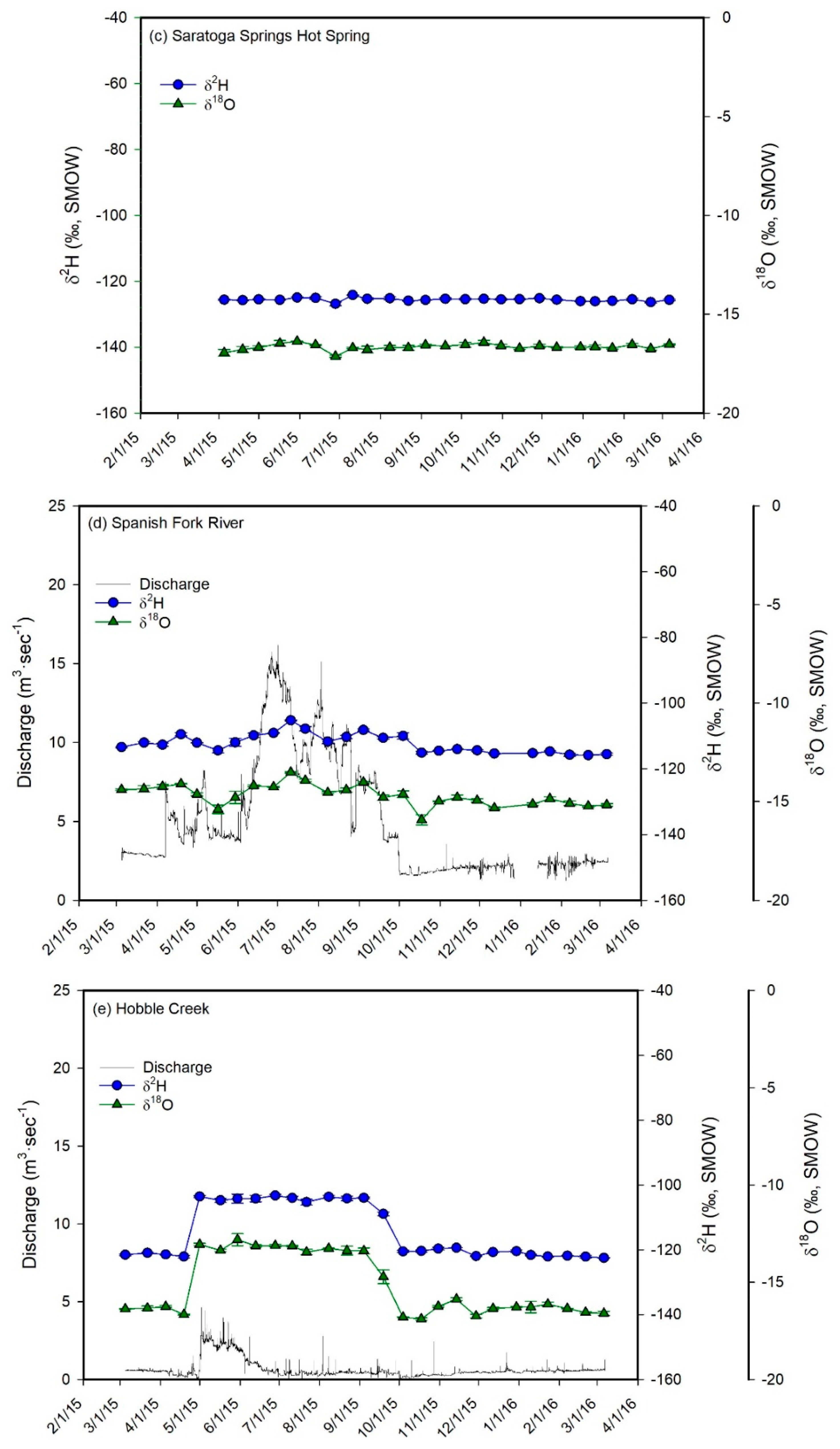
Similar to the well and hot spring waters, the δ²H and δ¹⁸O values of the inlets generally show a much smaller temporal variability compared to meteoric precipitation (Figure 5d,f,g). An exception is Hobble Creek, which shows higher δ-values during the irrigation season (Figure 5e). Average δ²H and δ¹⁸O values are, respectively, −112.3 ± 2.9‰ and −14.69 ± 2.40‰ (Spanish Fork River; Figure 5d), −114.4 ± 8.4‰ and −15.17 ± 1.58‰ (Hobble Creek; Figure 5e), −118.9 ± 0.9‰ and −16.07 ± 0.32‰ (Provo River; Figure 5f), −119.9 ± 1.4‰ and −16.54 ± 0.42‰ (American Fork River; Figure 5g). All the samples from the inlets plot on or close to the LMWL (Figure 6), suggesting that no significant evaporation occurs in these rivers and in the artificial reservoirs of the Central Utah Water Project (i.e., Deer Creek, Jordanelle, Strawberry, Currant Creek, Upper Stillwater, and Starvation reservoirs). We performed an isotope-based hydrograph separation to quantify the contribution of groundwater vs. meteoric precipitation in the inlets by applying the following equation:

$$X_{GW}=\frac{{\delta }_{River}-{\delta }_P}{{\delta }_{Gi}-{\delta }_P}$$

(22)

where X_GW is the average fraction of groundwater present in the stream flow, δ_River is the average δ²H or δ¹⁸O value of each inlet, δ_P is the amount-weighted average δ²H (−97.1‰) or δ¹⁸O (−13.59‰) value of meteoric precipitation, and δ_Gi is the average δ²H (−123.0‰) or δ¹⁸O (−16.33‰) value of all the well water samples (both the biweekly samples and the samples from the 111 shallow wells). Results (the average of δ²H and δ¹⁸O-derived values) are reported in Table 1 and indicate that the average fraction of groundwater present in stream flows during the study period (March 2015–March 2016) ranges from 0.49 (Spanish Fork River) to 0.98 (American Fork River).

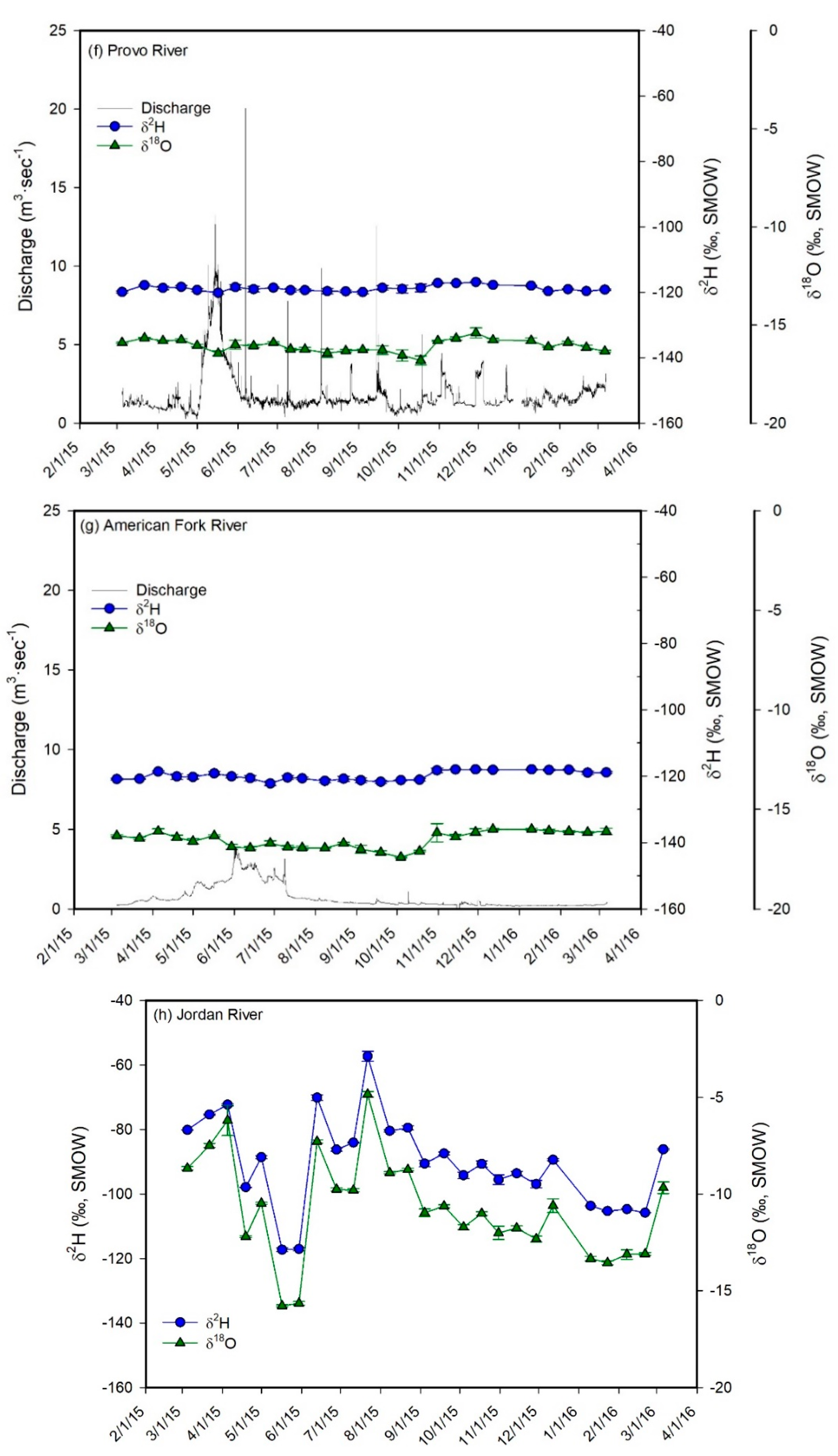
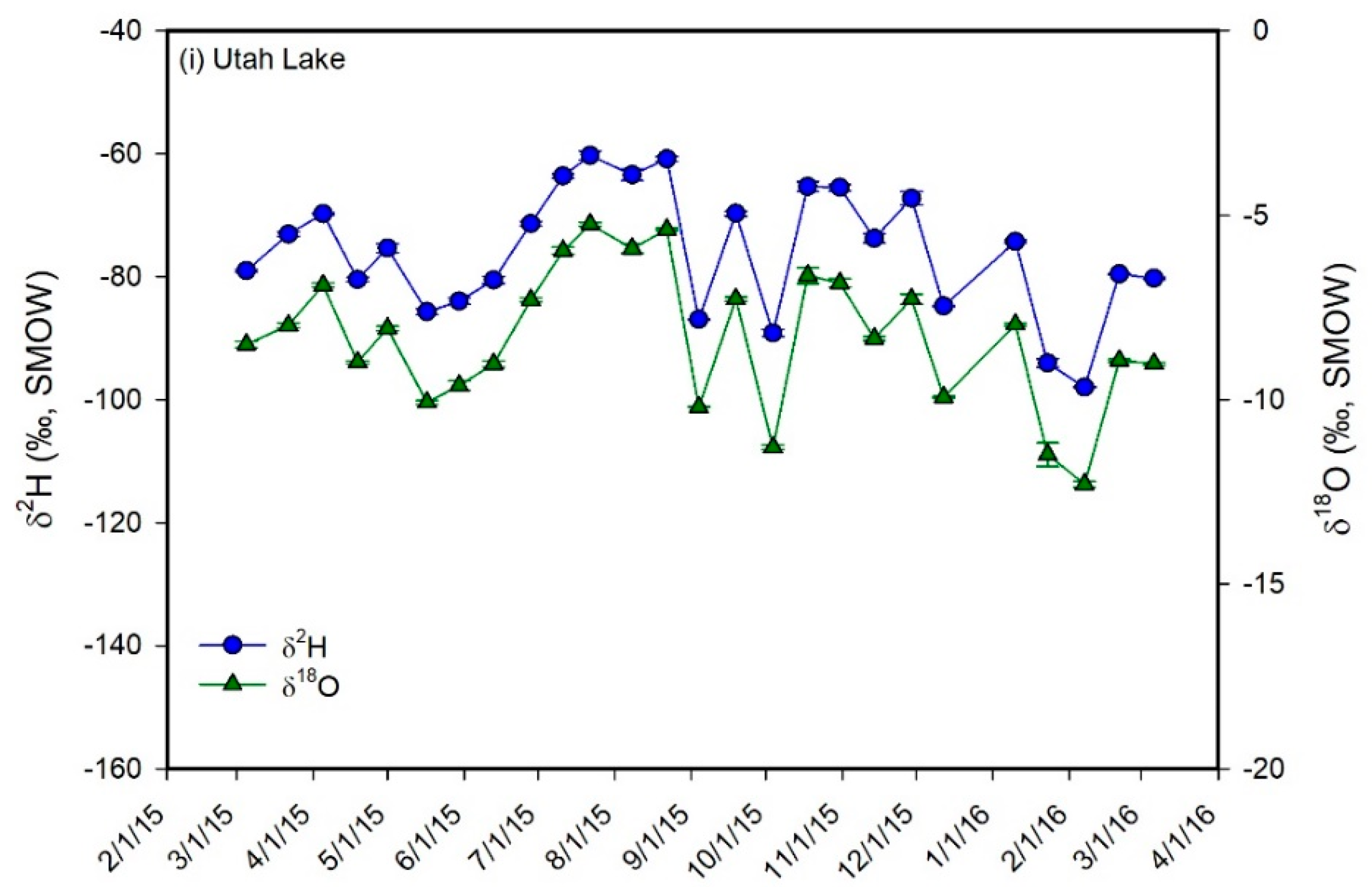
In contrast to the inlets, the samples from the Jordan River (average δ²H and δ¹⁸O of −90.4 ± 14.0‰ and −10.75 ± 2.66‰, respectively; Figure 5h), and from Utah Lake (average δ²H and δ¹⁸O of −76.0 ± 10.2‰ and −8.32 ± 1.87‰, respectively; Figure 5i) show much higher temporal variability and plot below the LMWL on local evaporation lines (LEL’s; Figure 6), suggesting that their water has undergone significant evaporation. The LEL for Utah Lake has following equation:

$$\delta 2H=\left(5.39\pm 0.08\right)·\delta 18O-\left(31.62\pm 0.75\right)$$

(23)

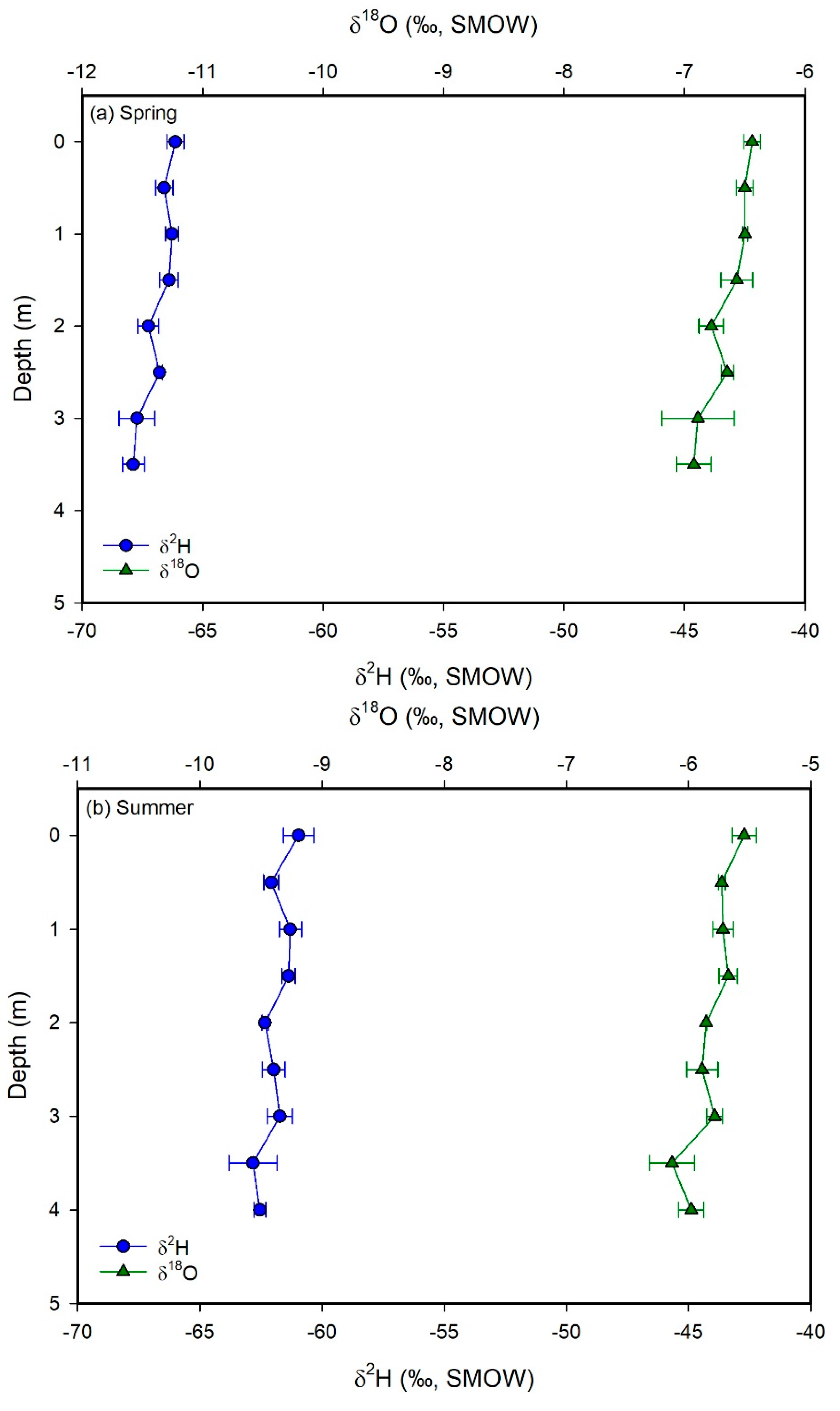
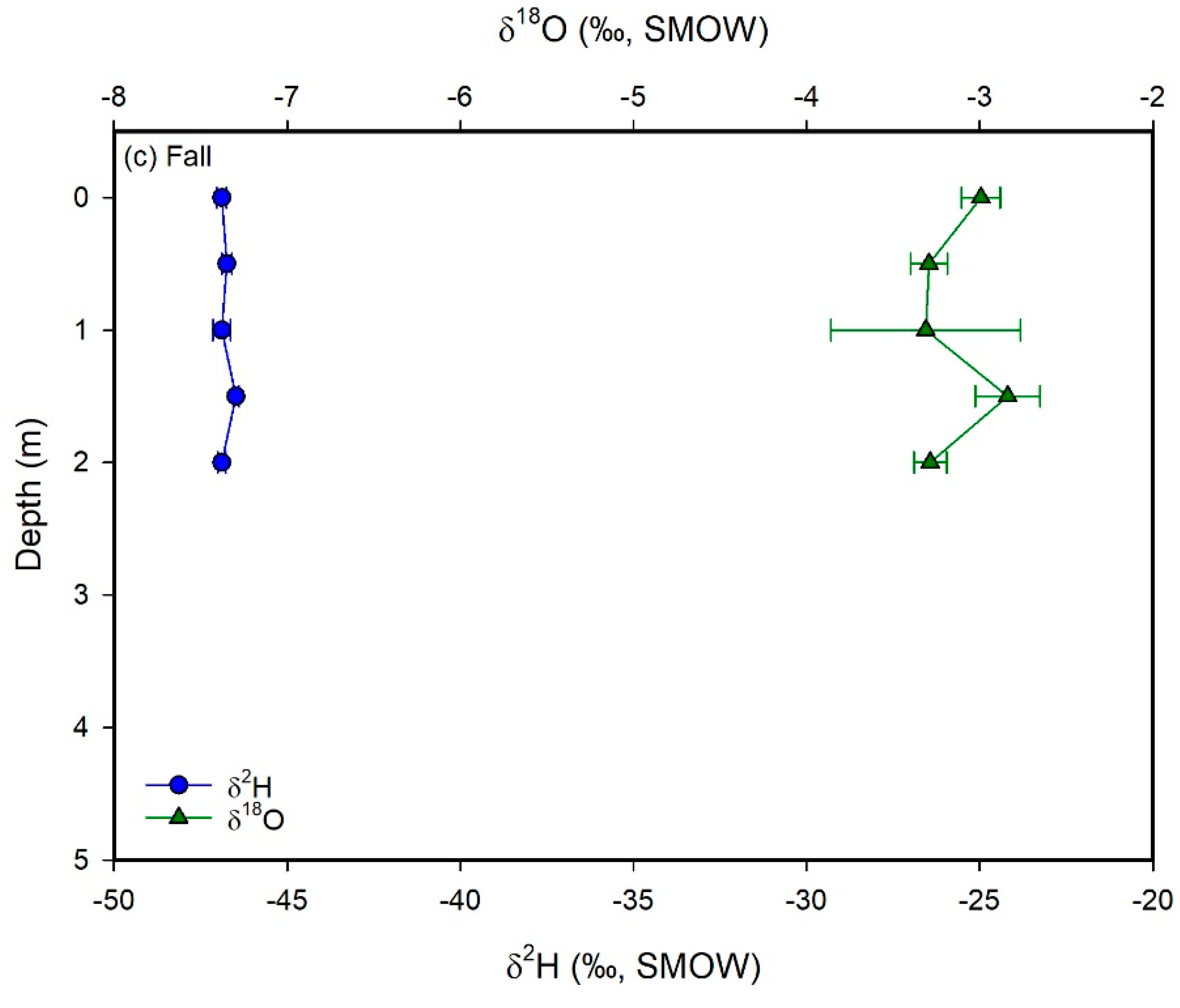
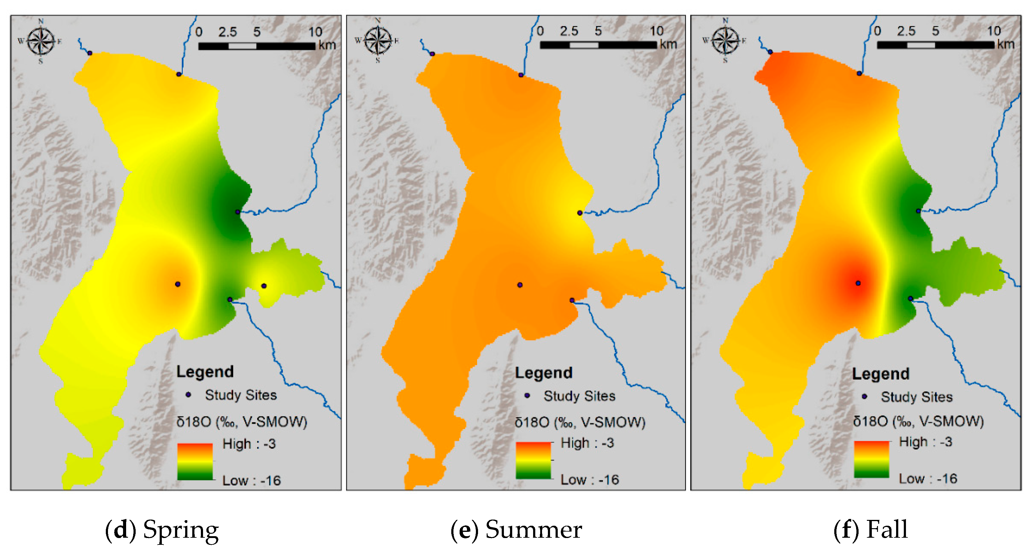
This equation is similar to those of other mountain lakes in the western US [48]. Vertical profiles show constant δ-values with depth (Figure 7). In contrast, surface water samples collected at different locations spread over the whole lake show very different δ-values, particularly in the spring and in the fall. The generally higher δ-values observed in the western part of the lake reflect evaporative enrichment in ¹⁸O and ²H as water moves away from the major inflow regions (Figure 8). These results suggest that the lake is well mixed vertically, but poorly mixed horizontally. We interpret these mixing patterns as a result of the physical characteristics and orientation of the lake, which is principally mixed by the wind. More specifically, the lake is too shallow for a thermocline to develop and the shear stress from the wind is conveyed to the bottom of the lake, mixing the entire water column vertically. With respect to the poor horizontal mixing, the lake is narrow and oriented N–S. As a result, winds blowing from the west (which is the predominant wind direction in the area) cannot develop much of a fetch (region of spatially homogeneous wave patterns) and each part of the lake is mixed to different degrees at different times. The difference in temperature and salinity of the water flowing into the lake from the inlets vs. the water that has resided in the lake for some time likely creates an additional density barrier to horizontal mixing. These observations suggest that dissolved chemicals will likely distribute uniformly in the water column. At the same time, however, different areas of the lake could potentially have different concentrations of chemicals. Consequently, pollutants derived from point sources—like wastewater treatment plants—will not be diluted easily throughout the lake. Indeed, phosphorous concentrations in the water column are higher in the eastern than in the western part of the lake [9].

To quantitatively characterize the hydrology of the lake, we applied the equations described in the materials and methods section to calculate the water balance parameters for the lake. These parameters are important because the water quality and biological conditions of a lake depend not only on local land use and disturbance to the lake and shores, but also on hydrological processes that link the surrounding landscape and climate to the lake [49].

Table 3. Input parameters used to calculate the throughflow index, the residence time of water, and the rate of groundwater inflow for Utah Lake using the equations of [34] and of [20]. See text for details.

Parameter	Value
Average Air Temperature in April—Nov. 2015 (T; °C)	14.50
Average Relative Humidity in April—Nov. 2015 (h)	0.53
Liquid Water-Water Vapor Kinetic Isotope Separation for H Isotopes (2εK; ‰)	6.25
Liquid Water-Water Vapor Equilibrium Isotope Separation for H Isotopes (2ε+; ‰)	91.02
Liquid Water-Water Vapor Kinetic Isotope Separation for O Isotopes (18εK; ‰)	7.10
Liquid Water-Water Vapor Equilibrium Isotope Separation for O Isotopes (18ε+; ‰)	10.28
Fractionation Factor for H Isotopes (2α+)	1.091023
Fractionation Factor for O Isotopes (18α+)	1.010284
Limiting H Isotope Composition of the Lake (δ2H*; ‰)	24.7
Limiting O Isotope Composition of the Lake (δ18O*; ‰)	13.46
m for H Isotopes (2m)	0.8105
m for O Isotopes (18m)	0.9519
Steady State H Isotope Composition of the Lake (δ2HL; ‰)	−69.3
Steady State O Isotope Composition of the Lake (δ18OL; ‰)	−7.15
H Isotope Composition of the Input Water (δ2HI; ‰)	−112.1
O Isotope Composition of the Input Water (δ18OI; ‰)	−15.17
Measured H Isotope Composition of Atmospheric Water Vapor (δ2HA; ‰)	−159.1
Measured O Isotope Composition of Atmospheric Water Vapor (δ18OA; ‰)	−21.56
Average Volume of Water in Utah Lake in Apr—Nov. 2015 (V; m3)	527,670,841
Average Rate of Evaporation from Utah Lake in Apr—Nov. 2015 (Er; mm·day−1)	5.53
Total Volume of Water Evaporated from Utah Lake in April—Nov. 2015 (E; m3)	396,187,719.4
Total Volume of Meteoric Precipitation Fallen on Utah Lake in April—Nov. 2015 (P; m3)	59,643,279
H Isotope Composition of Meteoric Precipitation (δ2HP; ‰)	−79.4
O Isotope Composition of Meteoric Precipitation (δ18OP; ‰)	−11.30
Total Volume of Surface Water Inflow in April-Nov. 2015 (Si; m3)	198,849,024
H Isotope Composition of the Surface Water Inflow (δ2HSi; ‰)	−114.5
O Isotope Composition of the Surface Water Inflow (δ18OSi; ‰)	−15.18
H Isotope Composition of the Groundwater Inflow (δ2HGi; ‰)	−123.0
O Isotope Composition of the Groundwater Inflow (δ18OGi; ‰)	−16.33
H Isotope Composition of Evaporating Water (δ2HE; ‰)	−186.9
O Isotope Composition of Evaporating Water (δ18OE; ‰)	−26.73

reports the values used in the equations to calculate the hydrological parameters. The throughflow index (E/I) is important because evaporation tends to increase the concentration of chemicals, leading to an increase in salinity, contaminants, and nutrient concentrations [50,51,52]. In US lakes, high values of E/I are generally associated with poor biological conditions [14]. In the calculation of E/I from Equations (5)–(9), for the δ_Is we used the values derived from the intersection of the LMWL with the lake’s LEL (δ²H = −111.8‰; δ¹⁸O = −154.87‰). For δ_Ls we used the average of the seasonal samples (δ²H = −69.3‰; δ¹⁸O = −7.15‰), which we expect to be more representative of the lake’s average composition than the biweekly samples, as they were collected from different locations in the lake. For temperature and relative humidity, we used the April to November 2015 average values recorded at the Provo Airport (T = 14.5 °C; h = 0.53). Finally, for δ_As we tried two different approaches. First, we calculated values assuming isotopic equilibrium between meteoric precipitation and atmospheric water vapor using the equation reported in [53]:

$${\delta }_A=\frac{{\delta }_P-{ϵ}^{+}}{{\alpha }^{+}}$$

(24)

where δ_A is the δ²H or δ¹⁸O value of atmospheric water vapor, δ_P is the evaporative-flux weighted average δ²H or δ¹⁸O value of meteoric precipitation (δ²H = −74.5‰; δ¹⁸O = −10.90‰), and ε⁺ and α⁺ are, respectively, the equilibrium isotope separations and fractionation factors between liquid water and water vapor. Using the equation above, we obtained δ_A values of −173.1‰ (δ²H) and −21.26‰ (δ¹⁸O). In a different approach, we used the April to October 2015 average δ_A values measured at the University of Utah (δ²H = −159.1‰; δ¹⁸O = −21.564‰; Richard Fiorella, personal communication). The results for E/I from the first approach are 0.68 and 0.39 using δ²H and δ¹⁸O data, respectively. Values of E/I obtained using the second approach are 0.56 (using δ²H) and 0.39 (using δ¹⁸O). The disagreement between the δ²H and the δ¹⁸O-derived values likely results from the scatter around the LEL and/or from the larger uncertainty associated with δ²H measurements. The disagreement between the calculated and measured values of δ_A suggests the presence of disequilibrium between atmospheric water vapor and meteoric precipitation, which is a common observation in arid and semi-arid regions [16,34,53,54,55,56]. However, an average of the two values obtained with the second approach (E/I = 0.47) is very similar or identical to previous estimates [3,13]. The high evaporation rate in the lake is likely a consequence of its shallowness, which facilitates the increase in temperature of the water column. Another contribution might come from the seiches that periodically form in the lake. These waves can wet large areas of the shore thereby increasing the amount of evapotranspiration [3].

The second parameter that we calculated is the water residence time. This parameter is critical for the health of a lacustrine ecosystem because it influences the concentrations of nutrients, oxygen, phytoplankton, zooplankton, suspended particles, and contaminants [57,58,59]. Most notably, for the same input, the concentration of dissolved nutrients and contaminants increases as the water residence time increases [60]. Indeed, observations conducted in other lakes indicate that the growth of harmful cyanobacteria increases as the water residence time increases [26]. Longer residence times may also increase the sedimentation rates and adsorption of toxic metals, reducing the concentration of, for instance, mercury, lead, zinc, and copper [61,62]. To calculate this parameter, we first calculated E_r (evaporation rate in mm·day⁻¹) using Equation (14) and obtained an average value for our study period of 5.53 mm·day⁻¹. We then obtained lake levels from the Utah Lake Commission [63] and calculated the average volume of the lake using Equation (2). The average lake level during the study period is 1367.03 m a.s.l. and the calculated volume is ~528 million m³. Plugging the E/I, E_r, and V calculated above in Equation (13) yields a value for the residence time of water in the lake of 154 days or 0.42 years. Note that “years” in this context refers to active water years and not calendar years. To calculate calendar years, it is necessary to account for the inactive winter season. Given that during most winters the lake is at least partially covered by ice for approximately three months, the water residence time in calendar years is ~25% longer (i.e., 193 days or 0.53 years). This result supports the observation that water residence time is correlated with lake depth, with shallow lakes having a shorter residence time than deep lakes [14].

The most difficult hydrological parameters to calculate in a lake water budget are certainly the groundwater inflow and outflow. Indeed, interactions between lakes and groundwater are not well understood. Quantifying the groundwater–lake hydrogeochemical interactions is important for water resource management, for understanding lacustrine ecology and nutrient balances, and for quantifying the vulnerability of lakes to pollution. Although most of the phosphorous in the lake appears to derive from geologic sources [64], groundwater could be an important source of nutrients, as observed in several other lakes [65,66,67,68]. Many cases have been reported where contaminants and/or nutrient-rich groundwater entering lakes has led to pollution and/or eutrophication [69,70,71]. To try to calculate the volume of groundwater inflow from Equation (17), for δ_L, we used the average δ-values of the seasonal lake samples (δ²H = −69.3‰; δ¹⁸O = −7.15‰), for δ_Ps the April to November 2015 average δ-values of meteoric precipitation weighted by amount (δ²H = −79.4‰; δ¹⁸O = −11.30‰), for δ_Sis the average δ-values of the inlets weighted by discharge (δ²H = −114.5‰; δ¹⁸O = −15.18‰), and for δ_Gis the average δ-values of all the well water samples (both the biweekly samples and the samples from the 111 shallow wells; δ²H = −123.0‰; δ¹⁸O = −16.33‰). We also calculated the isotope composition of the evaporative flux by applying Equation (18), obtaining values of −186.9‰ (δ²H) and −26.73‰ (δ¹⁸O). In terms of water volumes, for P we used the total volume of meteoric precipitation fallen on the lake surface during the study period (~60 million m³), for S_i and E, respectively, the total volume of water discharged by the inlets (~199 million m³·year⁻¹), and the total volume of water evaporated from the lake during the study period (~396 million m³·year⁻¹). Using these data, we estimated a value for G_i of ~689 million m³ (using δ²H data) and of ~644 million of m³ (using δ¹⁸O data). The average of the two values (~667 million m³ for our 8 month study period or ~1000 million m³·year⁻¹) is almost an order of magnitude higher than previous estimates based on a salt-balance model [1,3]. It is noteworthy that the USGS gauge of the Spanish Fork River is located far upstream at Castilla (Figure 3) and records the flow of the river before some irrigation diversions. As a result, our estimate of S_i is likely overestimated, although it does not account for the minor streams that discharge into the lake. Overestimating S_i would lead to an underestimation of G_i. Nevertheless, when normalized to the surface area of the lake, our Gi estimate for Utah Lake (0.9 cm·day⁻¹) is very similar to that reported for the nearby Great Salt Lake (0.8 cm·day⁻¹; [72]). Unfortunately, to our knowledge no gauge is currently set up to measure the streamflow of the Jordan River directly out of Utah Lake. All the gauges of the USGS and of the Utah Division of Water Rights are located further downstream and measure the discharge of the river after some of the water has been diverted into irrigation canals. As a result, an accurate estimate of the groundwater outflow using the residual of the hydrologic budget equation is not possible. However, we can use the discharge value reported in [64] and estimate a maximum value for G_o (G_o = ~177 million m³ for our 8 month study period or ~266 million m³·year⁻¹).

Table 4. Water budget for Utah Lake during the period April to November 2015. The outflow in the Jordan River is a minimum estimate (data from [64]) and the groundwater outflow is a maximum estimate.

Inflows	106 m3
Spanish Fork River	126.53
Provo River	38.80
American Fork River	19.29
Hobble Creek	14.23
Meteoric Precipitation	59.64
Groundwater	666.66
Total Inflows	925
Outflows
Evaporation	396.19
Jordan River	351.64
Groundwater	177.33
Total Outflows	925

shows the water budget for Utah Lake during the period April to November 2015. Although some of our assumptions may not be strictly correct for Utah Lake, these calculations provide a first-order approximation of water balance conditions and suggest that the rate of groundwater inflow estimated in previous studies might be underestimated. In addition, our results suggest that at least 72% of the total water input into the lake may derive from groundwater flow. From our data, Utah Lake appears therefore to be a groundwater-dominated lake. The dominance of groundwater inflow, the short residence time of water in the lake, and the precipitation of endogenic calcite (which is an effective process sequestering phosphorous into sediments) might suggest that the lake is relatively resilient to surface water anthropogenic disturbances.

Results from this study can help state agencies to responsibly manage the precious freshwater resources of Utah Valley. In addition, the stable isotope data provided here not only characterize the present-day lake system, but can also provide valuable input data for the reconstruction of past hydrologic and climatic conditions that are based on the stable isotope composition of lake sediment components, such as lacustrine cellulose and biogenic and endogenic carbonates. Most of the terrestrial isotope-based paleoclimate proxies rely on the reconstruction of the isotopic composition of meteoric precipitation, which at mid-latitudes depends on temperature [73]. These studies will have to consider that surface water bodies in Utah Valley are preferentially recharged by winter precipitation and that evaporation substantially changes the isotopic signal of the input water as the water resides in the lake.

To obtain a more accurate picture of the water balance in the lake, our recommendation for future studies includes conducting the sampling at higher spatial and temporal resolution and for a longer period of time. In addition, we recommend complementing the stable isotope method with and additional tracer (e.g., Cl⁻) and with additional techniques such as numerical models, seepage meters and piezometers, and radon 222. Radon 222 is a radioactive gas with short (3.8 days) half-life and residence time that is found only in lakes with active groundwater connections. Whereas stable isotope methods provide data on the average conditions during the entire water residence time, radon-based methods reflect a snapshot of groundwater flow representing a period of maximum 20 days. This technique can therefore be particularly helpful in the determination of the temporal variability of the groundwater flow into the lake.

4. Conclusions

New data are presented here on the hydrogen and oxygen stable isotope composition of water from the hydrologic system of Utah Lake (north–central Utah, USA), one of the largest natural freshwater lakes in the western US and a crucial water resource for the ~500,000 people living in Utah Valley. Our data suggest that:

(1)

Streamflow in the inlets (i.e., in the Spanish Fork River, Hobble Creek, Provo River, and American Fork River) is dominated by groundwater. In turn, groundwater is recharged by winter precipitation.

(2)

No significant evaporation occurs in the inlets or in the artificial reservoirs of the Central Utah Water Project (i.e., Deer Creek, Jordanelle, Strawberry, Currant Creek, Upper Stillwater, and Starvation reservoirs).

(3)

Utah Lake is affected by significant evaporation.

(4)

Utah Lake is well mixed vertically but poorly mixed horizontally.

(5)

In Utah Lake, during the period of April to November, ~47% of the total water inflow is lost by evaporation.

(6)

The residence time of water in Utah Lake is ~0.5 calendar years.

(7)

The volume of groundwater inflow to Utah Lake during the period April to November appears to be ~700 million m³. Groundwater inflow might contribute for the ~70% of the total water input to the lake. Utah Lake might therefore be a groundwater-dominated lake.

These results can help state agencies in the proper management of the lake in a challenging context of global climate change and rapid population growth. In addition, the stable isotope data from this study can provide a valuable modern analog for studies designed to reconstruct the paleoclimate and paleohydrology of the region from the stable isotope composition of lake sediments.

References

- PSOMAS. Utah Lake TMDL: Pollutant Loading Assessment & Designated Beneficial Use Impairement Assessment; PSOMAS: Los Angeles, CA, USA, 2007. [Google Scholar]
- Brimhall, W.H.; Merritt, L.B. Geology of Utah Lake: Implications for resource management. Great Basin Nat. Mem. 1981, 5, 24–42. [Google Scholar]
- Fuhriman, D.K.; Merritt, L.B.; Miller, A.W.; Stock, H.S. Hydrology and water quality of Utah Lake. Great Basin Nat. Mem. 1981, 5, 43–67. [Google Scholar]
- US Department of the Interior. Utah Lake Drainage Basin Water Delivery System. Available online: https://www.cupcao.gov/bonneville/uldbwds.html (accessed on 17 April 2020).
- Utah Division of Water Rights. Utah Lake Interim Water Distribution Plan. Available online: https://www.waterrights.utah.gov/wrinfo/policy/ut_lake/plan.htm (accessed on 20 April 2020).
- Baskin, R.L.; Spangler, L.E.; Holmes, W.F. Physical Characteristics and Quality of Water from Selected Springs and Wells in the Lincoln Point-Bird Island Area, Utah Lake, Utah; US Department of the Interior, US Geological Survey: Reston, WV, USA, 1994; Volume 93.
- Dustin, J.D. Hydrogeology of Utah Lake with emphasis on Goshen Bay: Provo, Utah. Ph.D. Thesis, Brigham Young University, Provo, UT, USA, 1978. [Google Scholar]
- Carling, G.T.; Tingey, D.G.; Fernandez, D.P.; Nelson, S.T.; Aanderud, Z.T.; Goodsell, T.H.; Chapman, T.R. Evaluating natural and anthropogenic trace element inputs along an alpine to urban gradient in the Provo River, Utah, USA. Appl. Geochem. 2015, 63, 398–412. [Google Scholar] [CrossRef] [Green Version]
- Randall, M.C.; Carling, G.T.; Dastrup, D.B.; Miller, T.; Nelson, S.T.; Rey, K.A.; Hansen, N.C.; Bickmore, B.R.; Aanderud, Z.T. Sediment potentially controls in-lake phosphorus cycling and harmful cyanobacteria in shallow, eutrophic Utah Lake. PLoS ONE 2019, 14, e0212238. [Google Scholar] [CrossRef]
- MacDonald, G.M. Water, climate change, and sustainability in the southwest. Proc. Natl. Acad. Sci. USA 2010, 107, 21256–21262. [Google Scholar] [CrossRef] [PubMed] [Green Version]
- Vörösmarty, C.J.; Green, P.; Salisbury, J.; Lammers, R.B. Global water resources: Vulnerability from climate change and population growth. Science 2000, 289, 284–288. [Google Scholar] [CrossRef] [PubMed] [Green Version]
- Beniston, M.; Stoffel, M. Assessing the impacts of climatic change on mountain water resources. Sci. Total Environ. 2014, 493, 1129–1137. [Google Scholar] [CrossRef] [PubMed]
- Merritt, L. Utah Lake, a Few Considerations. Unpubl. Lett. 3p 2004. [Google Scholar]
- Brooks, J.R.; Gibson, J.J.; Birks, S.J.; Weber, M.H.; Rodecap, K.D.; Stoddard, J.L. Stable isotope estimates of evaporation: Inflow and water residence time for lakes across the United States as a tool for national lake water quality assessments. Limnol. Oceanogr. 2014, 59, 2150–2165. [Google Scholar] [CrossRef] [Green Version]
- Jasechko, S.; Gibson, J.J.; Edwards, T.W. Stable isotope mass balance of the Laurentian Great Lakes. J. Great Lakes Res. 2014, 40, 336–346. [Google Scholar] [CrossRef]
- Gibson, J.; Reid, R. Water balance along a chain of tundra lakes: A 20-year isotopic perspective. J. Hydrol. 2014, 519, 2148–2164. [Google Scholar]
- Gibson, J.; Birks, S.; Jeffries, D.; Yi, Y. Regional trends in evaporation loss and water yield based on stable isotope mass balance of lakes: The Ontario Precambrian Shield surveys. J. Hydrol. 2017, 544, 500–510. [Google Scholar]
- Xiao, W.; Wen, X.; Wang, W.; Xiao, Q.; Xu, J.; Cao, C.; Xu, J.; Hu, C.; Shen, J.; Liu, S. Spatial distribution and temporal variability of stable water isotopes in a large and shallow lake. Isot. Environ. Health Stud. 2016, 52, 443–454. [Google Scholar] [CrossRef] [PubMed]
- Sacks, L.A.; Lee, T.M.; Swancar, A. The suitability of a simplified isotope-balance approach to quantify transient groundwater–lake interactions over a decade with climatic extremes. J. Hydrol. 2014, 519, 3042–3053. [Google Scholar] [CrossRef] [Green Version]
- Krabbenhoft, D.P.; Bowser, C.J.; Anderson, M.P.; Valley, J.W. Estimating groundwater exchange with lakes: 1. The stable isotope mass balance method. Water Resour. Res. 1990, 26, 2445–2453. [Google Scholar] [CrossRef]
- Isokangas, E.; Rozanski, K.; Rossi, P.; Ronkanen, A.-K.; Kløve, B. Quantifying groundwater dependence of a sub-polar lake cluster in Finland using an isotope mass balance approach. Hydrol. Earth Syst. Sci. 2015, 19, 1247–1262. [Google Scholar] [CrossRef] [Green Version]
- Yehdeghoa, B.; Rozanski, K.; Zojer, H.; Stichler, W. Interaction of dredging lakes with the adjacentgroundwater field: An isotope study. J. Hydrol. 1997, 192, 247–270. [Google Scholar] [CrossRef]
- Elmarami, H.; Meyer, H.; Massmann, G. Combined approach of isotope mass balance and hydrological water balance methods to constrain the sources of lake water as exemplified on the small dimictic lake Silbersee, northern Germany. Isot. Environ. Health Stud. 2017, 53, 184–197. [Google Scholar] [CrossRef]
- Longinelli, A.; Stenni, B.; Genoni, L.; Flora, O.; Defrancesco, C.; Pellegrini, G. A stable isotope study of the Garda lake, northern Italy: Its hydrological balance. J. Hydrol. 2008, 360, 103–116. [Google Scholar] [CrossRef]
- Pham, S.V.; Leavitt, P.R.; McGowan, S.; Peres-Neto, P. Spatial variability of climate and land-use effects on lakes of the northern Great Plains. Limnol. Oceanogr. 2008, 53, 728–742. [Google Scholar] [CrossRef] [Green Version]
- Romo, S.; Soria, J.; Fernandez, F.; Ouahid, Y.; Baron-Sola, A. Water residence time and the dynamics of toxic cyanobacteria. Freshw. Biol. 2013, 58, 513–522. [Google Scholar] [CrossRef]
- Gröning, M.; Lutz, H.O.; Roller-Lutz, Z.; Kralik, M.; Gourcy, L.; Pöltenstein, L. A simple rain collector preventing water re-evaporation dedicated for δ18O and δ2H analysis of cumulative precipitation samples. J. Hydrol. 2012, 448–449, 195–200. [Google Scholar]
- NCDC. Surface Data-Global Summary of the Day:1957–2009. Available online: http://www.ncdc.noaa.gov/ (accessed on 21 April 2020).
- United States Geological Survey. USGS Water Data for the Nation. Available online: https://waterdata.usgs.gov/nwis (accessed on 17 April 2020).
- Utah, T.U.o. Mesowest. Available online: https://mesowest.utah.edu/index.html (accessed on 17 April 2020).
- Wawro, P.R. Utah Lake Bathymetric Contour Lines. Available online: http://www.arcgis.com/home/item.html?id=03c0d9b15175479594acca6c6527fad4 (accessed on 17 April 2020).
- Topography, O. State of Utah Acquired LiDAR Data—Wasatch Front. Available online: https://portal.opentopography.org/datasetMetadata?otCollectionID=OT.122014.26912.1 (accessed on 17 April 2020).
- Dincer, T. The use of oxygen 18 and deuterium concentrations in the water balance of lakes. Water Resour. Res. 1968, 4, 1289–1306. [Google Scholar] [CrossRef]
- Gibson, J.J.; Birks, S.J.; Yi, Y. Stable isotope mass balance of lakes: A contemporary perspective. Quat. Sci. Rev. 2016, 131, 316–328. [Google Scholar] [CrossRef]
- Horita, J.; Wesolowski, D.J. Liquid-vapor fractionation of oxygen and hydrogen isotopes of water from the freezing to the critical temperature. Geochim. Cosmochim. Acta 1994, 58, 3425–3437. [Google Scholar] [CrossRef]
- Valiantzas, J.D. Simplified versions for the Penman evaporation equation using routine weather data. J. Hydrol. 2006, 331, 690–702. [Google Scholar] [CrossRef]
- Craig, H.; Gordon, L.I. Deuterium and Oxygen-18 Isotope Variations in the Ocean and Marine Atmosphere; Consiglio Nazionale delle Ricerche, Laboratorio di Geologia Nucleare: Pisa, Italy, 1965; p. 222. [Google Scholar]
- IAEA/WMO. Global Network of Isotopes in Precipitation. The GNIP Database. Available online: http://www.iaea.org/water (accessed on 28 August 2020).
- Craig, H. Isotopic variations in meteoric waters. Science 1961, 133, 1702–1703. [Google Scholar] [CrossRef]
- Hayes, J. Fractionation et al.: An introduction to isotopic measurements and terminology. Spectra 1982, 8, 3–8. [Google Scholar]
- Wilson, K.B.; Baldocchi, D.D. Seasonal and interannual variability of energy fluxes over a broadleaved temperate deciduous forest in North America. Agric. For. Meteorol. 2000, 100, 1–18. [Google Scholar] [CrossRef]
- Stahl, M.O.; Gehring, J.; Jameel, Y. Isotopic variation in groundwater across the conterminous United States–Insight into hydrologic processes. Hydrol. Process. 2020, 34, 3506–3523. [Google Scholar] [CrossRef]
- Winograd, I.J.; Riggs, A.C.; Coplen, T.B. The relative contributions of summer and cool-season precipitation to groundwater recharge, Spring Mountains, Nevada, USA. Hydrogeol. J. 1998, 6, 77–93. [Google Scholar] [CrossRef]
- Bowen, G. The online isotopes in precipitation calculator. Version OIPC 3.1. 2018. Available online: https://wateriso.utah.edu/waterisotopes/pages/data_access/form.html (accessed on 22 October 2020).
- McMahon, P.; Plummer, L.; Böhlke, J.; Shapiro, S.; Hinkle, S. A comparison of recharge rates in aquifers of the United States based on groundwater-age data. Hydrogeol. J. 2011, 19, 779. [Google Scholar] [CrossRef]
- Anderson, P.B. Hydrogeology of Recharge Areas and Water Quality of the Principal Aquifers Along the Wasatch Front and Adjacent Areas, Utah; US Department of the Interior, US Geological Survey: Reston, WV, USA, 1994; Volume 93.
- Sanjinez Guzman, V.A.; Langevin, C.P.; Richards, R.; Stockfleth, C.T.; Ulibarri, M.J.; Emerman, S.H. Hydrology of Big Spring, Fairfield, Utah: A Prelude to Native American Archaeology. In Proceedings of the GSA Annual Meeting 2017, Seattle, WA, USA, 22–25 October 2017. [Google Scholar]
- Henderson, A.K.; Shuman, B.N. Hydrogen and oxygen isotopic compositions of lake water in the western United States. GSA Bull. 2009, 121, 1179–1189. [Google Scholar] [CrossRef]
- Fraterrigo, J.M.; Downing, J.A. The influence of land use on lake nutrients varies with watershed transport capacity. Ecosystems 2008, 11, 1021–1034. [Google Scholar] [CrossRef]
- Anderson, N.J.; Harriman, R.; Ryves, D.; Patrick, S. Dominant factors controlling variability in the ionic composition of West Greenland lakes. Arct. Antarct. Alp. Res. 2001, 33, 418–425. [Google Scholar] [CrossRef]
- Wolfe, B.B.; Karst-Riddoch, T.L.; Hall, R.I.; Edwards, T.W.; English, M.C.; Palmini, R.; McGowan, S.; Leavitt, P.R.; Vardy, S.R. Classification of hydrological regimes of northern floodplain basins (Peace–Athabasca Delta, Canada) from analysis of stable isotopes (δ18O, δ2H) and water chemistry. Hydrol. Process. Int. J. 2007, 21, 151–168. [Google Scholar] [CrossRef]
- Sokal, M.A.; Hall, R.I.; Wolfe, B.B. Relationships between hydrological and limnological conditions in lakes of the Slave River Delta (NWT, Canada) and quantification of their roles on sedimentary diatom assemblages. J. Paleolimnol. 2008, 39, 533–550. [Google Scholar] [CrossRef]
- Skrzypek, G.; Mydłowski, A.; Dogramaci, S.; Hedley, P.; Gibson, J.J.; Grierson, P.F. Estimation of evaporative loss based on the stable isotope composition of water using Hydrocalculator. J. Hydrol. 2015, 523, 781–789. [Google Scholar] [CrossRef] [Green Version]
- Mercer, J.J.; Liefert, D.T.; Williams, D.G. Atmospheric vapour and precipitation are not in isotopic equilibrium in a continental mountain environment. Hydrol. Process. 2020, 34, 3078–3101. [Google Scholar] [CrossRef]
- Mayr, C.; Lücke, A.; Stichler, W.; Trimborn, P.; Ercolano, B.; Oliva, G.; Ohlendorf, C.; Soto, J.; Fey, M.; Haberzettl, T. Precipitation origin and evaporation of lakes in semi-arid Patagonia (Argentina) inferred from stable isotopes (δ18O, δ2H). J. Hydrol. 2007, 334, 53–63. [Google Scholar] [CrossRef]
- Fiorella, R.P.; West, J.B.; Bowen, G.J. Biased estimates of the isotope ratios of steady-state evaporation from the assumption of equilibrium between vapour and precipitation. Hydrol. Process. 2019, 33, 2576–2590. [Google Scholar] [CrossRef]
- Downing, B.D.; Bergamaschi, B.A.; Kendall, C.; Kraus, T.E.; Dennis, K.J.; Carter, J.A.; Von Dessonneck, T.S. Using continuous underway isotope measurements to map water residence time in hydrodynamically complex tidal environments. Environ. Sci. Technol. 2016, 50, 13387–13396. [Google Scholar] [CrossRef] [PubMed] [Green Version]
- Obertegger, U.; Flaim, G.; Braioni, M.G.; Sommaruga, R.; Corradini, F.; Borsato, A. Water residence time as a driving force of zooplankton structure and succession. Aquat. Sci. 2007, 69, 575–583. [Google Scholar] [CrossRef]
- Kaste, Ø.; Stoddard, J.L.; Henriksen, A. Implication of lake water residence time on the classification of Norwegian surface water sites into progressive stages of nitrogen saturation. Water Air Soil Pollut. 2003, 142, 409–424. [Google Scholar] [CrossRef]
- Lerman, A. Eutrophication and water quality of lakes: Control by water residence time and transport to sediments. Hydrol. Sci. J. 1974, 19, 25–34. [Google Scholar] [CrossRef]
- Selvendiran, P.; Driscoll, C.T.; Montesdeoca, M.R.; Choi, H.-D.; Holsen, T.M. Mercury dynamics and transport in two Adirondack lakes. Limnol. Oceanogr. 2009, 54, 413–427. [Google Scholar] [CrossRef] [Green Version]
- Rippey, B.; Rose, C.L.; Douglas, R.W. A model for lead, zinc, and copper in lakes. Limnol. Oceanogr. 2004, 49, 2256–2264. [Google Scholar] [CrossRef]
- Commission, U.L. Water Levels. Available online: http://utahlakecommission.org/water-levels/ (accessed on 17 April 2020).
- Abu-Hmeidan, H.Y.; Williams, G.P.; Miller, A.W. Characterizing total phosphorus in current and geologic utah lake sediments: Implications for water quality management issues. Hydrology 2018, 5, 8. [Google Scholar] [CrossRef] [Green Version]
- Belanger, T.; Mikutel, D.; Churchill, P. Groundwater seepage nutrient loading in a Florida lake. Water Res. 1985, 19, 773–781. [Google Scholar] [CrossRef]
- Kang, W.-J.; Kolasa, K.; Rials, M. Groundwater inflow and associated transport of phosphorus to a hypereutrophic lake. Environ. Geol. 2005, 47, 565–575. [Google Scholar] [CrossRef]
- Kidmose, J.; Nilsson, B.; Engesgaard, P.; Frandsen, M.; Karan, S.; Landkildehus, F.; Søndergaard, M.; Jeppesen, E. Focused groundwater discharge of phosphorus to a eutrophic seepage lake (Lake Væng, Denmark): Implications for lake ecological state and restoration. Hydrogeol. J. 2013, 21, 1787–1802. [Google Scholar] [CrossRef]
- Brock, T.D.; Lee, D.R.; Janes, D.; Winek, D. Groundwater seepage as a nutrient source to a drainage lake; Lake Mendota, Wisconsin. Water Res. 1982, 16, 1255–1263. [Google Scholar] [CrossRef]
- Hagerthey, S.E.; Kerfoot, W.C. Groundwater flow influences the biomass and nutrient ratios of epibenthic algae in a north temperate seepage lake. Limnol. Oceanogr. 1998, 43, 1227–1242. [Google Scholar] [CrossRef]
- Zhang, X.-J.; Chen, C.; Ding, J.-Q.; Hou, A.; Li, Y.; Niu, Z.-B.; Su, X.-Y.; Xu, Y.-J.; Laws, E.A. The 2007 water crisis in Wuxi, China: Analysis of the origin. J. Hazard. Mater. 2010, 182, 130–135. [Google Scholar] [CrossRef] [PubMed]
- Holman, I.P.; Whelan, M.J.; Howden, N.J.; Bellamy, P.H.; Willby, N.; Rivas-Casado, M.; McConvey, P. Phosphorus in groundwater—An overlooked contributor to eutrophication? Hydrol. Process. Int. J. 2008, 22, 5121–5127. [Google Scholar] [CrossRef]
- Anderson, R.; Naftz, D.; Day-Lewis, F.; Henderson, R.; Rosenberry, D.; Stolp, B.; Jewell, P. Quantity and quality of groundwater discharge in a hypersaline lake environment. J. Hydrol. 2014, 512, 177–194. [Google Scholar] [CrossRef]
- Rozanski, K.; Araguas-Araguas, L.; Gonfiantini, R. Isotopic paterns in modern global precipitation. In Climate Change in Continental Isotopic Records; American Geophysical Union: Washington, DC, USA, 1993; Volume 78, pp. 1–36. [Google Scholar]
Figure 1.
Map showing northern Utah and the geographic locations, landforms, and structures mentioned in the text.
Figure 2.
Average monthly temperature and precipitation during the study period compared to the climatology, i.e., the long-term (1981–2010) monthly averages for Utah Lake near Lehi [28]. Temperature and precipitation amounts were generally similar to the long-term average, but May and December 2015 and January 2016 were wetter, whereas February 2016 was drier than average.
Figure 3.
Location map showing the sampling sites of the biweekly samples, of the seasonal samples, of the meteoric precipitation (Utah Valley University: UVU), and of the 111 shallow groundwater wells. The figure also shows the location of the Provo Airport weather station (the source of the climate data) and of the USGS river gauges (the source of the discharge data).
Figure 4.
Linear correlation between lake volume and lake surface height in Utah Lake. The green dots show the lake volume calculated with ArcGIS corresponding to the lake heights of 1366.0, 1366.5, 1369.0, 1369.5, 1370.0, 1370.5, 1371 m.
Figure 5.
Plots of δ2H (blue circles) and δ18O (green triangles) values vs. time for the monthly water samples of meteoric precipitation (a) and for the biweekly water samples of the shallow groundwater well (b), hot spring (c), the inlets (d–g), the Jordan River (h), and Utah Lake (i). The plot for meteoric precipitation also shows the average monthly temperature and the monthly precipitation amounts. Error bars correspond to ± 1 sd. The samples from the inlets, from the well, and from the hot spring show a much lower temporal variability in δ-values than meteoric precipitation. In addition, their average values are similar to each other and to the values of winter precipitation, suggesting that groundwater is the main component in Utah Valley rivers and that aquifers in Utah Valley are predominantly recharged by snowmelt. The Jordan River and Utah Lake show higher average δ-values and a much higher temporal variability in δ-values than the inlets and groundwater.
Figure 6.
Plot of δ2H vs. δ18O values for the monthly water samples of meteoric precipitation, for all the samples of well water, and for the biweekly water samples of the hot spring, the inlets, the Jordan River, and Utah Lake. The plot also shows the local meteoric water line (LMWL) in blue with a 95% confidence band, the global meteoric water line, and the local evaporation line (LEL) for Utah Lake. Error bars correspond to ±1 sd. The samples from the inlets, from the wells, and from the hot spring plot on or close to the LMWL, indicating their meteoric origin and suggesting that significant evaporation did not occur in these water bodies. In contrast, water samples from the Jordan River and Utah Lake plot on the right of the LMWL along well-defined LEL’s indicating that their water underwent significant evaporation.
Figure 7.
Plots of δ2H (blue circles) and δ18O (green triangles) values vs. depth for Utah Lake water samples collected in the spring (a), summer (b), and fall (c) 2015. Error bars correspond to ± 1 sd. The δ-values show no significant variability with depth, suggesting that the lake is well-mixed vertically.
Figure 8.
Spatial variability in the δ2H (a–c) and δ18O (d–f) values of Utah Lake surface water samples collected in the spring, summer, and fall 2015. The δ-values were modeled using the inverse distance weighted interpolation spatial analysis method in Arc-GIS. The δ-values vary significantly over the lake surface (particularly in the spring and fall), suggesting that the lake is poorly mixed horizontally.